J. Mt. Sci.(2

Abstract: flooding understandprocesses orisk managhydrologicawave appmechanismuncertaintyfor flash flshallow wainfiltration.were modelThen the mflash floodscatchment model is shofairly well cdistributionmodelling omodel parahydrograph

Full 2Flood

HUAN

CAO Z

QI We

Garet

ZHAO

1 StatChin

2 Cha

3 Inst

4 Offi

5 Sha

CitatJourn

© Sc

Received: 30Accepted: 20

015) 12(5): 12

Mountain cadue to h

ding of the f flash floods

gement. Howal models basproximations

ms of flash floy. Here a hydrloods based ater equation Laboratory elled to illustra

model was apps of distinct in Shanxi Pown to be abl

compared to tn of rainfall iof flash floodmeters revea

hs are more

2D Hydrds

NG Wei1,2

Zhi-xian1

en-jun4 h

th PENDER3

O Kai5 http

te Key Laboratona

angjiang Water

titute for Infras

ice of Shanxi Pr

anxi Provincial H

tion: Huang Wnal of Mountain

cience Press and

0 January 2015 0 May 2015

03-1218

atchments arheavy rain

generation s is essential fwever, traditied on kinema

ignore coods and thurodynamic mon the full

ns incorporatexperiments oate the capabplied to resolmagnitudes

Province, Chile to reproducthe observed is shown to bds. Sensitivityal that the stae sensitive t

rodynam

http://orcid

http://orcid.o

http://orcid.or

3 http://orc

p://orcid.org/

ory of Water Re

rway Planning D

structure and En

rovincial Flood D

Hydrographic a

W, Cao ZX, Qi W Science 12(5). D

d Institute of M

re prone to ffall. Enhan

and evolufor effective flional distribuatic and diffu

certain physus bear exces

model is presentwo-dimensi

ting rainfall of overland flility of the mlve two obserin the Leng

ina. The prece the flood fldata. The sp

be crucial fory analyses of

age and dischto the Mann

mic Mo

.org/0000-00

org/0000-00

rg/0000-0003

cid.org/0000-

/0000-0001-6

esources and Hy

Design and Res

nvironment, He

Defense and Dr

and Water Reso

WJ, et al. (201DOI:10.1007/s1

ountain Hazard

e-mail: jms@

flash nced

ution flood uted

usion sical ssive nted onal and

lows model.

rved gkou esent lows atial

r the f the arge ning

routhanflasmodwhirainpersfor

KeySpa

Not

d =f =F =F ,

g =

h=

cHji,

delling

002-9235-336

01-5161-385X

3-2714-3223;

-0003-2265-8

6905-8567; e-

ydropower Eng

search Institute,

eriot-Watt Univ

rought Relief He

ources Survey B

15) Full 2D hyd11629-015-3466

ds and Environm

@imde.ac.cn

ghness and in to the Gre

sh flood augdelling resulich clearly cnfall in dicspectives, themodelling lar

ywords: Flaatial distributi

tations:

=distance; = the infiltrat=cumulative iG=are interfdirections re

=the accelerat

=water depth;

c =Green-Amp

j =the spatial directions re

of Rain

69; e-mail: hua

X; e-mail: zx

e-mail: qwj66

8228; e-mail: g

mail: 1350350

gineering Scienc

, Wuhan 430011

versity, Edinbur

eadquarters, Ta

Bureau, Taiyuan

drodynamic mo6-1

ment, CAS and S

DOI: 10

initial water ceen-Ampt heagments due lts agree witcharacterizes ctating the e proposed mrge flash flood

sh flood; Fullion; Rainfall

ion rate; infiltration deface fluxes in espectively; tion due to gr

;

pt capillary h

node indexesespectively;

nfall-ind

angvy@whu.ed

xcao@whu.edu

676@163.com

g.pender@hw

07540@163.co

ce, Wuhan Univ

1, China

rgh EH14 4AS,

aiyuan 030002

n 030001, Chin

odelling of rainf

Springer-Verlag

http://jm0.1007/s11629

content in thad. Most notto heavier r

th observed the paramo

floods. Frommodel is more

ds.

l hydrodynam

epth; the x - and y

ravity;

ead;

s in the x - an

duced F

du.cn

u.cn

w.ac.uk

om

versity, Wuhan

UK

, China

na

fall-induced fla

g Berlin Heidelb

ms.imde.ac.cn9-015-3466-1

1203

e catchment tably, as the rainfall, the data better,

ount role of m practical appropriate

mic model;

y -

nd y -

Flash

430072,

ash floods.

berg 2015

J. Mt. Sci.(2015)12(5): 1203-1218

1204

k =the time level;

sK =saturated hydraulic conductivity; n =Manning roughness; N =number of rain gauges;

xq , yq =unit discharges in the x - and y - directions

respectively; r =the rainfall intensity; R =precipitation; RSR= root mean error- observations standard

deviation ratio; PBIAS= percentage bias; S=the source term;

fS =friction source term;

sS =bed source term;

0S =additional bed source term;

U =a vector of conserved variables; u , v =velocity components in the x - and y -

directions respectively; z =bed elevation;

iθ =initial volumetric water content;

sθ =saturated volumetric water content;

bxτ , byτ =bed stresses in the x - and y - directions

respectively; tΔ = the time step; xΔ , yΔ =spatial steps in the x - and y - directions

respectively.

Introduction

Flash floods normally feature rapid onset (within a few hours of rainfall), which leaves very limited time for effective response. It is often accompanied by intense sediment transport (Reid et al. 1998) and other disasters such as debris flows and landslides (Aleotti 2004). Flash flooding is one of the most hazardous natural events, and is frequently responsible for loss of life and excessive damage to infrastructure and the environment (Jonkman 2005). According to the SFCDRH (2012), a single flash flood could lead to the loss of tens, even hundreds of lives. Thus, to mitigate the risk associated with flash floods, it is fundamental to understand catchment response to rainfall input, runoff generation and flood routing.

Hapuarachchi et al. (2011) divided existing models of rainfall-runoff forecasting into three

categories: data-driven models, lumped hydrological models and distributed hydrological models. Data-driven models use statistical relationships derived from rainfall and river flow data to generate flow forecasts. It is widely used for flood forecasting because of its simplicity. However, these models require long-term data records to train or calibrate the models and therefore it is not suitable for flash flood forecasting, since flash floods usually occur in small catchments in which gauged data is often rare or simply unavailable. Lumped hydrological models are primarily used for flood forecasting with the hypothesis of parameters invariant in space (Carpenter et al. 1999). In general, the usefulness of lumped hydrological models for flash flood is limited by their coarse resolution, the need for long-term historical data for calibration, and inapplicability to poorly gauged catchments (Hapuarachchi et al. 2011). Distributed models are gaining popularity among hydrologists in simulating the non-linear response of a watershed to rainfall events (Hunter et al. 2007; Reed et al. 2007; Javelle et al. 2010; Alfieri et al. 2012; Cools et al. 2012; Biondi and De Luca 2013). The basic physical principles are the conservation of mass and momentum for shallow water flows that are commonly known as the De Saint Venant equations. With different approximations to the shallow flow equations, the distributed models are divided into kinematic wave (Woolhiser and Liggett 1967; Liu and Singh 2004), diffusion wave (Ogden and Julien 1993, Philipp and Grundmann 2013), adaptive kinematic-dynamic model (Warnock et al. 2014) and full hydrodynamic models (Cao et al. 2010; Cea et al. 2010; Ballesteros Cánovas et al. 2011; Xia et al. 2011; Kim et al 2012; Berardi et al. 2013; Costabile et al. 2013). A comparative study has shown the inapplicability of kinematic and diffusion wave models to accurately resolve flash floods (Pan et al. 2012). Although some simplified models have been confirmed by the agreement between modelling results and observations, complete confirmation is logically precluded by the fallacy of affirming the consequent and by incomplete access to natural phenomena (Oreskes et al. 1994). Consequently, it is critical to develop flash flood models incorporating as much physical mechanism as possible, which seems to be the most viable way of

J. Mt. Sci.(2015)12(5): 1203-1218

1205

improving the reliability of numerical modelling (Cao et al. 2010; Costabile et al. 2013). Without incorporating the full mechanisms of flash flood flows, kinematic and diffusion wave approximations are unable to properly represent some specific flow structures (e.g. shock waves and hydraulic jumps). For example, while the kinematic wave approximation may be valid for simplified geometry, real watershed topography may lead to flows that are not always dominated by gravity and resistance which further results in infinite depth (Warnock et al. 2014). In contrast, full two dimensional (2D) hydrodynamic modelling currently features a sensible balance between theoretical rigour, which incorporates more physical mechanisms and thus increases complexity, and applicability, thanks to the recent advances in the creation of highly resolved catchment scale digital terrain models, the development of efficient numerical schemes, availability of high-power computing facility and also the fact that flash flooding usually occurs in relatively small catchments (typically several hundred square kilometers or less) and lasts for short periods of time (hours) (Cao et al. 2010).

Although hydrodynamic models have been applied to model flash floods, most of them focused on overland flows in laboratory experiments with rainfall and infiltration (Esteves et al. 2000), flood propagation and the related inundation in the river systems with neither rainfall nor infiltration processes (Xia et al. 2011; Ballesteros Cánovas et al. 2011) or flash floods in the urban areas only with rainfall process (Cea et al. 2010). Cao et al. (2010) presented one of the first full hydrodynamic modelling studies of flash floods in real catchments incorporating both rainfall and infiltration. Yet no field observed data was available to test the modelling. Berardi et al. (2013) applied the full 2D hydrodynamic models, the commercial software Wallingford InfoWorks-RS, to model flash flood in ephemeral streams in Southern Italy. In their work, spatially and temporally uniform net-rainfall intensity over the entire catchment was assumed and no infiltration process was considered. Costabile et al. (2013) developed a 2D full hydrodynamic model for flash floods and applied it to an observed flash flood event. But no infiltration was involved and the net-rainfall intensity was employed instead.

To date, full hydrodynamic modelling studies of flash floods in a real catchment with both rainfall and infiltration are meagre, especially when field observed data is available for evaluating the modelling results. The present paper presents a full 2D hydrodynamic model for flash floods with both rainfall and infiltration. The model is first tested against two experiments of overland flow with/without infiltration. Then it is employed to model two flash floods of distinct magnitudes in the Lengkou catchment in Shanxi Province, China. Observed data is used to assess the model performance. Sensitivity to the model parameters (e.g., roughness, initial water content and the Green-Ampt head) and the estimation of the spatial rainfall distribution are evaluated.

1 Full Hydrodynamic Model

1.1 Governing equations

The full 2D hydrodynamic model in the present work is essentially an adapted version of the recent hydro-sediment-morphodynamic model of Huang et al. (2012), in which the sediment transport and bed evolution are neglected while the rainfall and infiltration are incorporated. It is built upon the 2D shallow water hydrodynamic equations. The pre-balanced governing equations are written in the conserved form as

SGFU =∂∂+

∂∂+

∂∂

yxt (1)

where U is a vector of conserved variables, )(UF and )(UG are convective flux vectors of the flow in the x - and y - directions respectively, )(US is the source term.

⎥⎥⎥

⎦

⎤

⎢⎢⎢

⎣

⎡

=

y

x

qqη

U ,

⎥⎥⎥

⎦

⎤

⎢⎢⎢

⎣

⎡

−+=huv

zghuhu

)2(5.0 22 ηηF ,

⎥⎥⎥

⎦

⎤

⎢⎢⎢

⎣

⎡

−+=

)2(5.0 22 zghvhuvhv

ηηG , (2a-c)

J. Mt. Sci.(2015)12(5): 1203-1218

1206

⎥⎥⎥⎥⎥⎥⎥⎥

⎦

⎤

⎢⎢⎢⎢⎢⎢⎢⎢

⎣

⎡

−∂

∂−

−∂

∂−

−

=

ρ

τη

ρτ

η

by

bx

y

zg

x

zg

fr

S (2d)

where η is the water surface level above the datum; z is bed elevation (the water depth then is evaluated by h = z−η ); u and v are velocity components in the x - and y - directions respectively; xq = hu and yq = hv are unit discharge in the x - and y - directions respectively; r is the rainfall intensity; f is the infiltration rate; g is the acceleration due to gravity; bxτ and byτ are bed stresses in the x - and y - directions

respectively.

1.2 Model closure

To close the governing equations, empirical relationships are introduced to estimate bed stresses and infiltration. The Manning's roughness coefficient n is used to calculate the bed stresses (Huang et al. 2012)

3/7222 /hqqqgn yxxbx += ρτ ,

3/7222 / hqqqgn yxyby += ρτ

(3a, b)

The Manning roughness is related to topography, land use and land cover and its values vary from region to region. For a real catchment, the Manning roughness is usually different in channels and in the rest domains. Moreover, from physical considerations, the roughness should increase when the flow is shallower compared to surface roughness elements (Barros and Colello 2001).

Although the infiltration rate f can be calculated using a plethora of empirical relationships (Kale and Sahoo 2011), the original Green-Ampt infiltration equation (Green and Ampt 1911) is used here

⎥⎦

⎤⎢⎣

⎡ −+==

F

HK

dt

dFf cis

s

)(1

θθ (4)

where sK is saturated hydraulic conductivity; cH is Green-Ampt capillary head, which is mainly determined by the soil type; sθ is saturated volumetric water content, which is usually set to be equal to soil porosity; iθ is initial volumetric water content; F is cumulative infiltration depth. The parameters are determined mainly through information on soil type, which are assumed to be constant where field data are not available. The initial volumetric water content iθ may vary spatially. However, it is hard to obtain the information about the spatial distribution of the initial water content for real flash floods. Following Martina et al. (2006), three values of the initial volumetric water content are adopted as 1/3, 2/3 and 1.0 of sθ , corresponding to dry, moderate wet and wet soil condition respectively.

1.3 Numerical schemes

The Godunov-type finite volume method in conjunction with Harten-Lax-van Leer Contact Wave (HLLC) approximate Riemann solver is used to solve the governing equations based on fixed rectangular meshes. The MUSCL (Monotone Upstream-centered Schemes for Conservation Laws) method is adopted to reconstruct the face values of the Riemann problem to achieve a second order in space (Toro 2001). Overall, the present model is improved over Cao et al. (2010) in that it is well balanced and can properly deal with the transition of wetting and drying interface. The numerical scheme is detailed in Huang et al. (2013) and only outlined below

1,,

*,

+Δ+= kjfi

kjiji tSUU (5)

xt jijijikji Δ−Δ−= −++ /)( *

,2/1,2/1*,

1, FFUU

kjsijiji tyt ,

*2/1,2/1, /)( SGG Δ+Δ−Δ− −+ (6)

where the superscript k represents the time level and the superscript ∗ indicates the state after calculating variables from Equation (5), subscript ( ji, ) are the spatial node indexes, tΔ is the time step, xΔ and yΔ denote the spatial steps, ji ,2/1+F ,

ji ,2/1−F , 2/1, +jiG and 2/1, −jiG are interface fluxes. In Equation (5), the friction source term

1+kfS

is solved by a splitting implicit method and limited value of the friction force is defined to ensure stability at the wet-dry interface (Liang and Marche

J. Mt. Sci.(2015)12(5): 1203-1218

1207

2009). When evaluating 1,+kjiU in Equation (6), the

solution of Equation (5) is used as the initial condition. The interface fluxes ji ,2/1+F , ji ,2/1−F ,

2/1, +jiG and 2/1, −jiG are computed using HLLC Riemann solver (Toro 2001), which necessitates reconstruction of the values of the Riemann states. The MUSCL reconstruction method in conjunction with the Minmod slope limiter is adopted to obtain the face values of the Riemann states. It should be noted that the slope-limited reconstruction is only applicable to those wet cells away from the wet-dry interface. In a dry or a wet cell next to a dry cell, the face values are set to be equal to those at the centers to give a stable representation of the wet-dry fronts.

The bed slope term ksS is discretized using the

method proposed by Liang and Marche (2009). The procedure for the x -direction is outlined below, while that for the y -direction is similar. For the dry bed case, two additional terms are employed in order to preserve a well-balanced solution:

jijisx SSx

zgS ,2/10,2/10 +− ++

∂

∂−= η (7)

The first term in the right hand side of Equation (7) is discretized as

)( ,2/1,2/1

x

zzg

x

zg jiji

Δ

−−=

∂

∂− −+ηη (8)

where 2/)( ,2/1,2/1L

jiR

ji +− += ηηη , the other two

terms are evaluated by:

.2

)(

,2

)(

,2/1,2/1,2/1,2/1,2/10

,2/1,2/1,2/1,2/1,2/10

x

zzzzgS

x

zzzzgS

jijijijiji

jijijijiji

Δ

−Δ−Δ=

Δ

Δ−−Δ=

−++++

−−+−−

(9a, b)

where

)).(,0max(

)),(,0max(

,2/1,2/12/1

,2/1,2/12/1

jiL

jii

jiR

jii

zz

zz

+++

−−−

−−=Δ

−−=Δ

η

η (10a, b)

Based on Equation (4), an implicit equation for F can be derived

⎟⎟⎠

⎞⎜⎜⎝

⎛−

+−+=)(

1ln)(isc

iscs HFHtKF

θθθθ

(11)

It is solved by iteration using the bisection method (Corliss 1977) because Equation (11) increases monotonously if t >0. Once F is known at any time, the infiltration rate f can be attained by Equation (4).

1.4 Boundary conditions

Reasonable implementation of boundary conditions is crucial for modelling flash floods in catchments. Esteves et al. (2010) suggested that no boundary condition is required as the flow at the outlet was supercritical; however, subcritical and supercritical flows could appear alternatively in complex catchment terrain (Cao et al. 2010). Another simple method is that flow variables on the boundary are set to be equal to those of the adjacent inward boundaries on the assumption of zero gradient between the neighboring layers. This method is extensively employed since it is easy to implement, whilst it is not generally physically justified (Jain et al. 2004). In the present study, the uncertainty of the boundary condition is minimized by obviating the need for boundary conditions, following Cao et al. (2010). Specifically, the computational domain is defined to include the whole catchment, and extends sufficiently beyond it so that the flood flow would have not arrived at the boundary of the computational domain during the time period of computation. Under this treatment, at the boundary of the computational domain, flow vanishes as it does in practice (i.e., no velocity and flow depth).

In the evaluation of the model, the computational results are compared to observed data collected in laboratory experiments and in the field. To quantify the overall difference between a numerical solution and observed data, the root-mean-square error to observations standard deviation ratio (RSR) and the percentage bias (PBIAS) indexes are chosen since there is explicit classified standard to evaluate the model efficiencies. RSR is estimated as the ratio of the root-mean-square error to the standard deviation of measured data using Equation (12). RSR varies from the optimal value of 0.0, which indicates vanishing RMSE or residual variation and therefore perfect model simulation, to a large positive value. PBIAS measures the average tendency of the model predicted values to be larger

J. Mt. Sci.(2015)12(5): 1203-1218

1208

or smaller than their corresponding measured values. Positive values indicate model underestimation bias, and negative values indicate model overestimation bias (Parajuli et al. 2009).

∑

∑

=

=

−

−=

Nn

ioi

N

ioici

YY

YYRSR

1

2

1

2

)(

)(,

∑

∑ ×−=

=

=n

ioi

N

icioi

Y

YYPBIAS

1

1100)(

(12a, b)

where oY and cY are the observed and computed values at instants i ; Y is the mean value of observed values for the entire period of the event; and N is the number of observed instants.

2 Model test against laboratory experiments

The present model has been tested against several cases without rainfall and infiltration (Huang et al. 2012), which have illustrated that the model can preserve the well-balanced property, capture shock waves and handle the wet/dry interface transition. Here two laboratory experiments are modelled to illustrate the capability of present model in reproducing rainfall-runoff processes.

2.1 Overland flow without infiltration

The experiments carried out by Iwagaki (1955) were widely used to validate rainfall-runoff models (e.g., Fiedler and Ramirez 2000; Costabile et al. 2013). The experiments consisted of a rainfall-runoff case over a cascade of three smooth aluminum plates. Each section was 8 m long, with slopes equal to 0.02, 0.015 and 0.01 in the downstream directions. The rainfall intensities were 0.108, 0.0638 and 0.08 cm/s over the three sections respectively. There was no infiltration during the experiment. Although three rainfall durations were considered in the experiments (10, 20 and 30 s), the case of 10 s duration is considered herewith because a shock wave and hydraulic jump were observed. The transmissive

boundary condition is applied at the outlet cross section (Liao et al. 2007). The Manning roughness suggested by Iwagaki (1955) was 0.009 s/m1/3. A mesh with xΔ =0.05 m is adopted in the modelling. Figure 1 shows the computed flow depth and discharge hydrographs at the outlet of the flume ( x =24 m) as compared against the observed data (Iwagaki 1955). It is seen that the maximum flow depth computed by present model is very close to the observed, while the timing of its occurrence is a little delayed (Figure 1a). Also the discharge hydrograph agrees with the observed rather well, whereas the peak discharge is a little overestimated (Figure 1b). Quantitatively, the values of RSR for depth and discharge hydrographs are 0.3475 and 0.4152 respectively, while the values of PBIAS for depth and discharge hydrographs are -1.92% and -7.71%. Overall, the computed flow depth and discharge hydrographs agree with experimental data very good or excellent.

2.2 Overland flow with infiltration

Overland flow experiments were conducted by de Lima (1992) in a 1.0×0.5 m flume with a slope 0.1. The uniform rainfall intensity was 3.741×10-5 m/s and lasted 15 minutes. The parameters for the Green-Ampt infiltration model were uniform along the flume and were specified to sK =1.67×10-5 m/s, sθ =0.506, iθ =0.0107, cH =0.02 m. The

computational mesh with xΔ =0.1 m is used and transmissive boundary condition is applied at the outlet cross section. Figure 2 shows that the computed unit-width discharge hydrograph by present model agrees well with the observed data. Quantitatively, the values of RSR and PBIAS of discharge hydrograph are 0.50 and 0.83% respectively. It is also shown that the discrepancies exist between the computed and observed discharge hydrographs at the rapidly rising and

Figure 1 Computed depth and discharge hydrographs compared against experiment data.

J. Mt. Sci.(2015)12(5): 1203-1218

1209

receding phases, which may be due to the neglect of the surface ponding capability (Liu and Singh 2004).

The modelling results for experiments with or without infiltration has illustrated that the model can reproduce the rainfall-runoff and the infiltration processes fairly well.

3 Model Test against Field Observed Data

3.1 Flash floods in Lengkou Catchment

The Lengkou catchment (35 21' ~35 26' N; 110 31' ~110 39' E) is located in southern Shanxi Province, China (Figure 3a). The catchment lies in a semi-humid area and its soil mainly consists of loess (DWRSP 2010). The area of this catchment is 76 km2, the main channel length upstream of the outlet cross section is 17 km, and the average streamwise bed slope of the main channel is 1/400. There are three classes of land cover in the Lengkou catchment: bust wood (14.1 km2), forest (61.4 km2) and loess (0.5 km2). The last several decades have seen land use changes, and yet no detailed data is available to quantify the changes. There are six rain gauges inside or in the immediate vicinity to the catchment, which are Lengkou, Yanzhuang, Hugeta, Xigou, Wangjialing and Henglinguan (as illustrated in Figure 3b). Two flood events, the 31st July 1996 flood and the 7th August 1982 flood, are studied here using the present hydrodynamic model. The DEM is 30 m ×

Figure 2 Computed discharge hydrograph and measured data.

Figure 3 (a) Location of Lengkou Catchment; (b) DEM of Lengkou Catchment and rain gauges distribution; (c) Topography of outlet cross section.

(a)

(b)

J. Mt. Sci.(2015)12(5): 1203-1218

1210

30 m, which is accessed through the Geospatial Data Cloud, Computer Network information Center, CAS (http://www.gscloud.cn). The highest peak and lowest elevation is 1591 m and 510 m in the computational domain (Figure 3) and the datum elevation is 585 m at the outlet cross section. The DEM of the computational domain (Figure 3b) is much larger than that of the catchment (as outlined by the dot line) to avoid the need for boundary conditions (as stated in the section 1.4).

One of the basic impediments to rainfall-runoff modelling in observed catchments is the lack of information of water flow at the initial state. Depressions such as lakes, pools and reservoirs may accommodate a large amount of water and should be filled at the initial state. Otherwise, much of the rainfall will come and be retained in the depressions during the rainfall-runoff process. In the context of hydrologic modelling, the DEM is deliberately changed by filling the depressions so that they are “hydrologically correct” (Zhu et al. 2013). However, the topography is critically important for overland flows and river flows in the context of full hydrodynamic model, the change of the topography may considerably alter the rainfall-runoff processes of flash flood. Here to estimate the initial water flow information as accurately as possible, the depressions are filled by water as the result of antecedent rainfall. The proposed model is applied to model the rainfall-runoff process under presumed antecedent rainfall without considering infiltration or subsurface flow. When the computed stage and discharge at the outlet cross-section match the observed data, the information of water flow in the catchment is used as the initial condition. This is in essence similar to Miyata et al. (2010) in an experimental study of overland flows in forests.

The saturated hydraulic conductivity for the Lengkou catchment is specified as sK =1.38 mm/hour (DWRSP 2010). The saturated volumetric water content sθ in Lengkou catchment ranges from 0.47 to 0.49 according to Wang (2010) and its average value is adopted here, i.e., sθ =0.48. The initial volumetric water content iθ may vary spatially. However, it is hard to obtain for the two floods studied here because these two floods occurred 17 and 31 years ago respectively. Following Martina et al. (2006), three values of the

initial volumetric water content are adopted as 1/3, 2/3 and 1.0 of sθ (i.e., s =1/3, 2/3 and 1.0), corresponding to dry, moderate wet and wet soil condition respectively.

The Manning roughness is related to topography, land use and land cover and its values vary from region to region. Unfortunately, there is no information about land use or land cover for the two floods, thus a unique value of Manning roughness has to be adopted in the whole catchment.

The spatial distribution of rainfall is important for flash flood modelling and it can be implemented by a variety of approaches (Goovaerts 2000; Li and Heap 2011), such as the Tiessen polygons and the inverse distance weighted (IDW) interpolation. The Thiessen polygons approach is herewith applied for the two observed flash floods, except otherwise specified.

For the Lengkou catchment, the location of the outlet cross section is shown in Figure 3b and the cross section is illustrated in Figure 3c, with P1 and P2 indicating the edge points of the river channel. To facilitate modelling assessment, the stage and discharge hydrographs at the outlet cross section are evaluated as compared to observed data.

Numerical tests are conducted to evaluate the sensitivity of the computational results to model parameters (e.g., cH , n and s ) and the implementation of the spatial distribution of rainfall in the following sections.

3.2 The 31st July 1996 Flood

The flood occurred on 31st July 1996 and the rainfall started at 10:00 ( t =10 hour) on 31st July. Stage rise of the flood at the outlet cross section began at 14:42 ( t =14.7 hour) and the flood duration was about 10 hours. The initial discharge at the outlet cross section was 3.19 m3/s.

3.2.1 Results

The parameters are calibrated to be cH =0.2 m, n =0.025 s/m1/3 and 3/1/ == sis θθ . In this subsection, all the computed results are based on these calibrated values. Figure 4 shows the precipitation process, and computed and observed stage and discharge hydrographs. It is seen that the precipitation varied significantly in space and in time (Figure 4). Figure 4a illustrates that the

J. Mt. Sci.(2015)12(5): 1203-1218

1211

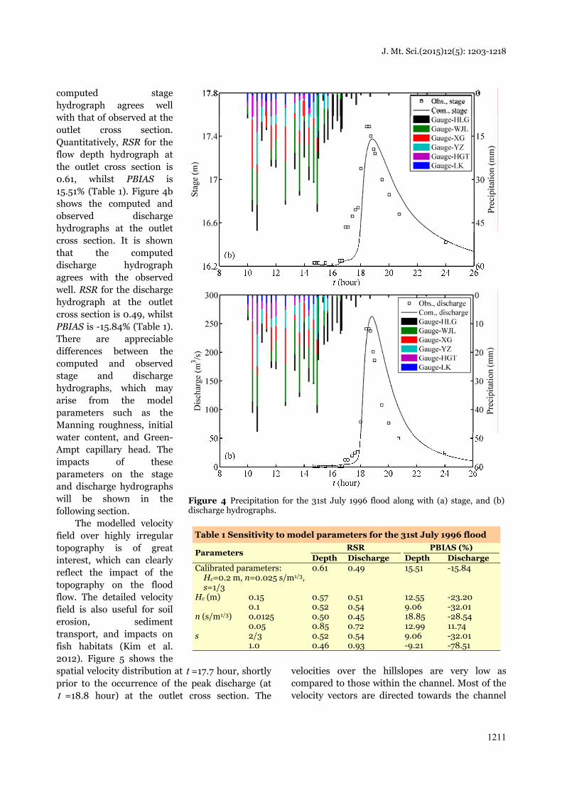
computed stage hydrograph agrees well with that of observed at the outlet cross section. Quantitatively, RSR for the flow depth hydrograph at the outlet cross section is 0.61, whilst PBIAS is 15.51% (Table 1). Figure 4b shows the computed and observed discharge hydrographs at the outlet cross section. It is shown that the computed discharge hydrograph agrees with the observed well. RSR for the discharge hydrograph at the outlet cross section is 0.49, whilst PBIAS is -15.84% (Table 1). There are appreciable differences between the computed and observed stage and discharge hydrographs, which may arise from the model parameters such as the Manning roughness, initial water content, and Green-Ampt capillary head. The impacts of these parameters on the stage and discharge hydrographs will be shown in the following section.

The modelled velocity field over highly irregular topography is of great interest, which can clearly reflect the impact of the topography on the flood flow. The detailed velocity field is also useful for soil erosion, sediment transport, and impacts on fish habitats (Kim et al. 2012). Figure 5 shows the spatial velocity distribution at t =17.7 hour, shortly prior to the occurrence of the peak discharge (at t =18.8 hour) at the outlet cross section. The

velocities over the hillslopes are very low as compared to those within the channel. Most of the velocity vectors are directed towards the channel

Figure 4 Precipitation for the 31st July 1996 flood along with (a) stage, and (b) discharge hydrographs.

Table 1 Sensitivity to model parameters for the 31st July 1996 flood

Parameters RSR PBIAS (%)

Depth Discharge Depth DischargeCalibrated parameters:

Hc=0.2 m, n=0.025 s/m1/3, s=1/3

0.61 0.49 15.51 -15.84

Hc (m) 0.15 0.57 0.51 12.55 -23.200.1 0.52 0.54 9.06 -32.01

n (s/m1/3) 0.0125 0.50 0.45 18.85 -28.540.05 0.85 0.72 12.99 11.74

s 2/3 0.52 0.54 9.06 -32.011.0 0.46 0.93 -9.21 -78.51

J. Mt. Sci.(2015)12(5): 1203-1218

1212

from the hill slopes, characterizing the accumulative process of the channel flood flow. Additionally, the velocities in the narrow reach of the channel are apparently higher than those in the wider reach. Further, no nonphysical (unrealistically high) velocity is discerned, which essentially reflects the satisfactory performance of the present model from numerical perspective.

3.2.2 Sensitivity analysis

The Green-Ampt capillary head is an important parameter in determining the infiltration rate (Equation 4). Liu and Singh (2004) adopted cH ranging from 0.02 m to 0.15 m for different cases. According to Chen and Young (2006), cH ranges from 0.05 m to 0.32 m, while Li and Heap (2011) suggested that it ranged from 0.13 m to 0.50 m. Here, three values (0.1 m, 0.15 m and 0.2 m) are used to examine the impact of the

Green-Ampt head on the stage and discharge hydrographs. The results are shown in Figure 6. Generally, the larger the cH , the lower the peak stage and peak discharge at the outlet. Comparatively, the rising phase of the stage and discharge hydrographs at the outlet is more sensitive to the cH than the receding phase. The stage and discharge start to rise earlier with respect to a smaller cH (Figure 6), and vice versa. Quantitatively, if cH decreases from 0.2 to 0.15 m and 0.1 m, RSR of the flow depth hydrograph decreases from 0.61 to 0.57 and 0.52, while PBIAS of the flow depth hydrograph decrease from 15.5% to 12.55% and 9.06%. Also, RSR of the discharge hydrograph increases from 0.49 to 0.51 and 0.54, while PBIAS of the discharge hydrograph decreases from -15.84% to -23.20% and -32.01%.

The Manning roughness plays a central role in flood modelling. Here it is tuned by -50% and +100% of the calibrated value n =0.025 s/m1/3 (Table 1). Figure 7 shows that the stage and discharge hydrographs at the outlet start to rise earlier in relation to a smaller Manning roughness, and vice versa. Also, the peak stage is higher with a larger Manning roughness (Figure 7a), whilst the peak discharge is smaller (Figure 8b). Quantitatively, if the Manning roughness changes to 0.0125 s/m1/3 and 0.05 s/m1/3 respectively, RSR of the flow depth hydrograph varies to 0.5 and 0.85 respectively, and PBIAS of the depth hydrograph changes to 18.85% and 12.99% accordingly (Table 1). Also, RSR of the discharge hydrograph varies to 0.45 and 0.72 respectively, and PBIAS of the discharge hydrograph changes to -28.54% and 11.74% respectively (Table 1).

Figure 5 Velocity distribution at t =17.7 hour.

Figure 6 Impact of Green-Ampt capillary head on (a) stage, and (b) discharge hydrographs for the 31st July 1996

flood.

J. Mt. Sci.(2015)12(5): 1203-1218

1213

The initial volumetric water content iθ is critical for determining the infiltration rate. Figure 8 shows the impacts of iθ on stage and discharge hydrographs. It is seen that stage and discharge hydrographs start to rise earlier with respect to a higher initial water content (or a larger s ). Figure 8a shows that the peak stage is higher in relation to a larger s . Similarly, Figure 8b shows that the peak discharge is larger with a larger s . This clearly echoes the physical reasoning that initial water content in the soil will exacerbate the flash flooding. Quantitatively, RSR of the flow depth hydrograph decreases from 0.61 to 0.52 and 0.46, while RSR of the discharge hydrograph increases from 0.49 to 0.54 and 0.93 (Table 1).

Similarly, PBIAS of the flow depth hydrograph decreases from 15.51% to 9.06% and -9.21%, while

PBIAS of the discharge hydrograph decreases from -15.84% to -32.01% and -78.51% (Table 1).

The sensitivity analysis has demonstrated that the Manning roughness and initial water content have considerable impacts on the stage and discharge hydrographs, whilst that of the Green-Ampt head is relatively minor.

3.2.3 Impact of Spatial Distribution of Precipitation

In addition to the Thiessen polygons approach, IDW interpolation is another common approach to determining the spatial distribution of precipitation (Goovaerts 2000; Li and Heap 2011). The precipitation at each cell is calculated

by ∑∑=

−

=

−=N

i

pii

N

i

pi dRdR

11/ , where id is the distance

Figure 7 Impact of Manning roughness on (a) stage, and (b) discharge hydrographs for the 31st July 1996 flood.

Figure 8 Impact of initial water content on (a) stage, and (b) discharge hydrographs for the 31st July 1996 flood.

J. Mt. Sci.(2015)12(5): 1203-1218

1214

from the cell to the i -th rain gauge; iR is the

precipitation of the i -th rain gauge; N is the total number of rain gauges; and p is an empirical exponent. The results from the present modelling exercises (not shown) indicate that it is critical to specify an appropriate exponent p if the IDW is to be used to determine the spatial distribution of precipitation in flash flood modelling. This essentially echoes the finding of Ogden and Julien (1993) derived from a modelling study based on the diffusion wave approximation, in which the impact of infiltration on the rainfall-runoff processes was ignored.

3.3 The 7th August 1982 Flood

In addition to the 31st July 1996 flood studied above, a flash flood of a smaller magnitude is modelled and evaluated here. It occurred on 7 August 1982, with a peak discharge 80.8 m3/s, which was approximately one third of the 31st July 1996 flood (241 m3/s). The initial discharge at the outlet cross section was 1.86m3/s.

3.3.1 Results

The parameters are calibrated to cH =0.2 m, n =0.05 s/m1/3 and initially the soil was moderately wet, i.e., 3/2/ == sis θθ . The modelling results in this subsection are all based on these calibrated values of model parameters.

Figure 9 shows the precipitation processes at six rain gauges and stage

and discharge hydrographs at the outlet cross section. It is shown that the precipitation varied largely in space and in time. The rainfall began at 12:00 ( t =12 hour) on 7th August 1982. For example, the precipitation between 14:00 and 16:00 was 51.3 mm at Gauge Hugeta (HGT), while that was 26.4 mm at Gauge Lengkou during the same period. The precipitation between 14:00 and 15:00 was 46.8 mm at Gauge Yanzhuang, while that was 0.4 mm between 15:00 and 16:00 at the same rain gauge. The significant variability means that high spatial and temporal resolution of the precipitation data is crucial if the flood is to be modelled reasonably well. As shown in Figure 9a, the computed stage hydrograph agrees with the observed qualitatively. Quantitatively, RSR for the flow depth hydrograph at the outlet cross section is 0.85, whilst PBIAS is -33.43% (Table 2). From Figure 9b it is seen that the computed discharge hydrograph is qualitatively in agreement with the observed. RSR for the discharge hydrograph at the outlet cross section is 0.66, whilst PBIAS is -59.95% (Table 2). Overall, considerable discrepancies exist between the computed and observed stage and discharge hydrographs.

Table 2 Sensitivity to model parameters for the 7th August 1982 flood

Parameters RSR PBIAS (%)

Depth Discharge Depth DischargeCalibrated parameters: Hc =0.2 m, n =0.05 s/m1/3, s =2/3

0.85 0.66 -33.43 -59.95

Hc (m) 0.15 0.88 0.70 -40.53 -66.090.1 0.92 0.74 -43.06 -73.39

n (s/m1/3) 0.025 0.86 1.07 -25.87 -103.070.075 0.96 0.77 -41.75 -24.51

s 1/3 0.75 0.61 -31.35 -40.801.0 1.13 1.02 -53.9 -105.88

Figure 9 Precipitation for the 7th August 1982 flood along with (a) stage, and (b) discharge hydrographs.

J. Mt. Sci.(2015)12(5): 1203-1218

1215

3.3.2 Sensitivity analysis

The impacts of the Green-Ampt head, Manning roughness and initial water content on stage and discharge hydrographs are evaluated. Figure 10 shows the impact of the Green-Ampt head on the stage and discharge hydrographs. It is seen that with a larger cH the stage and discharge hydrographs start to rise latter and the peak stage and peak discharge become smaller (Figure 10). It is noted that the Green-Ampt head affects little on the decreasing phase of the discharge hydrograph because the cumulative infiltration depth is so large that the infiltration rate is close to the saturated hydraulic conductivity. Quantitatively, as cH decreases from 0.2 m to 0.15 m and 0.1 m, the average RSR of the depth hydrograph increases from 0.85 to 0.88 and 0.92, while RSR of the discharge hydrograph increases from 0.66 to 0.70 and 0.74. The PBIAS values also vary

accordingly, as shown in Table 2. Figure 11 illustrates the impact of the Manning

roughness on the stage and discharge hydrographs at the outlet cross section. In line with a reduced Manning roughness, the peak stage is lower, the discharge hydrograph starts to rise earlier and the peak discharge is higher (Figure 11b); and vice versa. Quantitatively, as the Manning roughness changes to 0.025 s/m1/3 and 0.075 s/m1/3 respectively, the average RSR of the depth hydrograph increases from 0.85 to 0.86 and 0.96, while RSR of the discharge hydrograph changes to 1.07 and 0.77 respectively. In accord with these changes, the PBIAS values vary accordingly (Table 2).

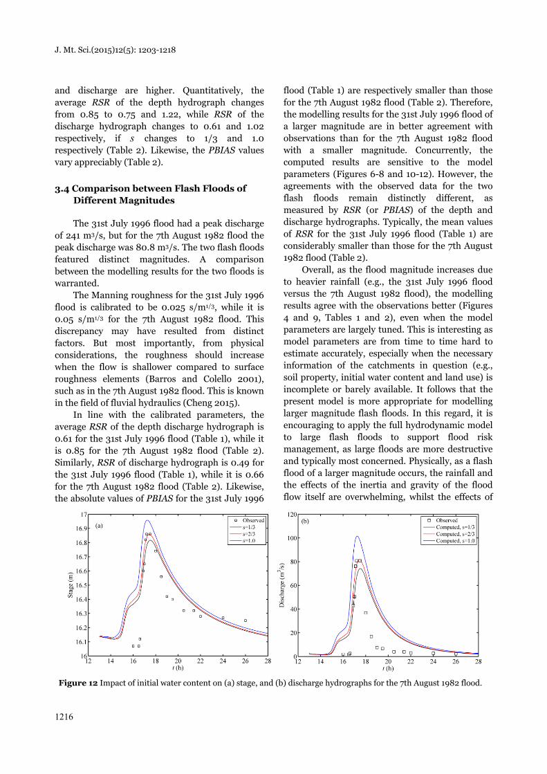
Figure 12 shows the impact of the initial water content on the stage and discharge hydrographs at the outlet cross section. With respect to larger initial water content the stage and discharge hydrographs start to rise earlier and the peak stage

Figure 10 Impact of Green-Ampt capillary head on (a) stage, and (b) discharge hydrographs for the 7th August 1982 flood.

Figure 11 Impact of Manning roughness on (a) stage, and (b) discharge hydrographs for the 7th August 1982 flood.

J. Mt. Sci.(2015)12(5): 1203-1218

1216

and discharge are higher. Quantitatively, the average RSR of the depth hydrograph changes from 0.85 to 0.75 and 1.22, while RSR of the discharge hydrograph changes to 0.61 and 1.02 respectively, if s changes to 1/3 and 1.0 respectively (Table 2). Likewise, the PBIAS values vary appreciably (Table 2).

3.4 Comparison between Flash Floods of Different Magnitudes

The 31st July 1996 flood had a peak discharge of 241 m3/s, but for the 7th August 1982 flood the peak discharge was 80.8 m3/s. The two flash floods featured distinct magnitudes. A comparison between the modelling results for the two floods is warranted.

The Manning roughness for the 31st July 1996 flood is calibrated to be 0.025 s/m1/3, while it is 0.05 s/m1/3 for the 7th August 1982 flood. This discrepancy may have resulted from distinct factors. But most importantly, from physical considerations, the roughness should increase when the flow is shallower compared to surface roughness elements (Barros and Colello 2001), such as in the 7th August 1982 flood. This is known in the field of fluvial hydraulics (Cheng 2015).

In line with the calibrated parameters, the average RSR of the depth discharge hydrograph is 0.61 for the 31st July 1996 flood (Table 1), while it is 0.85 for the 7th August 1982 flood (Table 2). Similarly, RSR of discharge hydrograph is 0.49 for the 31st July 1996 flood (Table 1), while it is 0.66 for the 7th August 1982 flood (Table 2). Likewise, the absolute values of PBIAS for the 31st July 1996

flood (Table 1) are respectively smaller than those for the 7th August 1982 flood (Table 2). Therefore, the modelling results for the 31st July 1996 flood of a larger magnitude are in better agreement with observations than for the 7th August 1982 flood with a smaller magnitude. Concurrently, the computed results are sensitive to the model parameters (Figures 6-8 and 10-12). However, the agreements with the observed data for the two flash floods remain distinctly different, as measured by RSR (or PBIAS) of the depth and discharge hydrographs. Typically, the mean values of RSR for the 31st July 1996 flood (Table 1) are considerably smaller than those for the 7th August 1982 flood (Table 2).

Overall, as the flood magnitude increases due to heavier rainfall (e.g., the 31st July 1996 flood versus the 7th August 1982 flood), the modelling results agree with the observations better (Figures 4 and 9, Tables 1 and 2), even when the model parameters are largely tuned. This is interesting as model parameters are from time to time hard to estimate accurately, especially when the necessary information of the catchments in question (e.g., soil property, initial water content and land use) is incomplete or barely available. It follows that the present model is more appropriate for modelling larger magnitude flash floods. In this regard, it is encouraging to apply the full hydrodynamic model to large flash floods to support flood risk management, as large floods are more destructive and typically most concerned. Physically, as a flash flood of a larger magnitude occurs, the rainfall and the effects of the inertia and gravity of the flood flow itself are overwhelming, whilst the effects of

Figure 12 Impact of initial water content on (a) stage, and (b) discharge hydrographs for the 7th August 1982 flood.

J. Mt. Sci.(2015)12(5): 1203-1218

1217

the characteristic parameters (e.g., initial water content, friction and soil porosity) of the catchment become relatively minor.

4 Conclusion

A full 2D hydrodynamic model is proposed for modelling flash floods due to rainfall. The model is first tested against two experiments. It is applied to model two observed flash floods in Lengkou Catchment, Shanxi Province in China. It is demonstrated that the observed stage and discharge hydrographs can be reproduced fairly well by the present model. The spatial distribution of rainfall is crucial for flash flood modelling even in the small catchment, which clearly necessitates refined rainfall gauging. The Manning roughness and initial water content have considerable impacts on the stage and discharge hydrographs, whilst that of the Green-Ampt head is relatively minor. Most

notably, for a larger flash flood induced by heavier rainfall, the modelling results agree with observed data better despite the largely tuned model parameters, which clearly characterizes the paramount role of rainfall in dictating the floods. Practically, the proposed model is encouragingly more appropriate for modelling large flash floods. To minimize the uncertainties aroused from the evaluation of model parameters, more information such as spatial distributions of land use/cover, soil types, spatial distribution of initial water content are required.

Acknowledgements

The research is funded by Natural Science Foundation of China (Grants Nos. 51279144 and 11432015) and also Chinese Academy of Sciences (Grant No. KZZD-EW-05-01-03).

Reference

Aleotti P (2004) A warning system for rainfall-induced shallow failures. Engineering Geology 73(3-4): 247-265. DOI: 10.1016/j.enggeo.2004.01.007

Alfieri L, Thielen J, Pappenberger F (2012) Ensemble hydro-meteorological simulation for flash flood early detection in southern Switzerland. Journal of Hydrology 424-425: 143-153. DOI: 10.1016/j.jhydrol.2011.12.038

Ballesteros Cánovas JA, Eguibar M, Bodoque JM, et al. (2011) Estimating flash flood discharge in an ungauged mountain catchment with 2D hydraulic models and dendrogeomorphic palaeostage indicators. Hydrological Processes 25(6): 970-979. DOI:10.1002/hyp.7888

Barros AP, Colello JD (2001) Surface roughness for shallow overland flow over crushed stone surfaces. Journal of Hydraulic Engineering 127(1): 38-52. DOI:10.1061/(ASCE) 0733-9429(2001)127:1(38)

Berardi L, Laucelli D, Simeone V, et al. (2013) Simulating floods in ephemeral streams in Southern Italy by full-2D hydraulic models. International Journal of River Basin Management 11(1): 1-17. DOI: 10.1080/15715124.2012.746975

Biondi D, De Luca DL (2013) Performance assessment of a Bayesian Forecasting System (BFS) for real-time flood forecasting. Journal of Hydrology 479: 51-63.DOI: 10.1016/ j.jhydrol.2012.11.019

Cao Z, Wang X, Zhang S, et al. (2010) Hydrodynamic modelling in support of flash flood warning. Proceedings of the ICE - Water Management 163(7): 327-340. DOI:10.1680/wama. 2010.163.5.255

Carpenter T, Sperfslage J, Georgakakos K, et al. (1999) National threshold runoff estimation utilizing GIS in support of operational flash flood warning systems. Journal of Hydrology 224(1): 21-44. DOI: 10.1016/S0022-1694(99) 00115-8

Cea L, Garrido M, Puertas J, et al. (2010) Overland flow

computations in urban and industrial catchments from direct precipitation data using a two-dimensional shallow water model. Water Science and Technology 62(9): 1998-2008. DOI:10.2166/wst.2010.746

Chen L, Young MH (2006) Green-Ampt infiltration model for sloping surfaces. Water Resources Research 42(7): 1-9. DOI:10.1029/2005WR004468

Cheng N (2015) Resistance Coefficients for Artificial and Natural Coarse-Bed Channels: Alternative Approach for Large-Scale Roughness. Journal of Hydraulic Engineering, 141(2): 040140721-040140727. DOI: 10.1061/(ASCE)HY.1943 -7900.0000966

Cools J, Vanderkimpen P, El Afandi G, et al. (2012) An early warning system for flash floods in hyper-arid Egypt. Natural Hazards and Earth System Science 12(2): 443-457. DOI: 10.5194/nhess-12-443-2012

Corliss G (1977) Which root does the bisection algorithm find? SIAM Review 19(2): 325-327.

Costabile P, Costanzo C, Macchione F (2013) A storm event watershed model for surface runoff based on 2D fully dynamic wave equations. Hydrological Processes 27(4): 554-569. DOI:10.1002/hyp.9237

de Lima JLMP (1992) Model KININF for overland flow on pervious surfaces. In: Parson T, Abrahams A (eds.), Overland Flow: Hydraulics and Erosion Mechanics. UCL Press, London, UK. pp 69-88.

DWRSP (Department of Water Resources of Shanxi Province) (2010) Handbook of hydrological calculation of Shanxi Province. Yellow River Conservancy Press, Zhengzhou, China. pp 136-137. (In Chinese)

Esteves M, Faucher X, Galle S, et al. (2000) Overland flow and infiltration modelling for small plots during unsteady rain: numerical results versus observed values. Journal of Hydrology 228(3-4): 265-282. DOI:10.1016/S0022-1694

J. Mt. Sci.(2015)12(5): 1203-1218

1218

(00)00155-4 Fiedler FR, Ramirez JA (2000) A numerical method for

simulating discontinuous shallow flow over an infiltrating surface. International Journal for Numerical Methods in Fluids 32(2): 219-239. DOI:10.1002/(SICI)1097-0363 (20000130)32:2<219::AID-FLD936>3.0.CO;2-J

Goovaerts P (2000) Geostatistical approaches for incorporating elevation into the spatial interpolation of rainfall. Journal of Hydrology 228(1–2): 113-129. DOI:10.1016/S0022-1694 (00)00144-X

Green WH, Ampt G (1911) Studies on soil physics, part 1: the flow of air and water through soils. Journal of Agricultural Science 4(1): 1-24.

Hapuarachchi HAP, Wang QJ, Pagano TC (2011) A review of advances in flash flood forecasting. Hydrological Processes 25(18): 2771-2784. DOI:10.1002/hyp.8040

Huang W, Cao Z, Yue Z, et al. (2012) Coupled modelling of flood due to natural landslide dam breach. Proceedings of the ICE - Water Management 165(10): 525-542. DOI:10.1680/wama. 12.00017

Huang W, Cao Z, Carling P, et al. (2013) 2D modelling of megaflood due to glacier dam-break in Altai Mountains, Southern Siberia. Proceedings of 35th IAHR, September 8-13, Chengdu, China.

Hunter NM, Bates PD, Horritt MS, et al. (2007) Simple spatially-distributed models for predicting flood inundation: A review. Geomorphology 90(3–4): 208-225. DOI:10.1016/ j.geomorph.2006.10.021

Iwagaki Y (1955) Fundamental Studies on the Runoff by Characteristics. Bulletins - Disaster Prevention Research Institute, Kyoto University. Vol 10, pp 1-25.

Jain MK, Kothyari UC, Ranga Raju KG (2004) A GIS based distributed rainfall–runoff model. Journal of Hydrology 299(1–2): 107-135. DOI:10.1016/j.jhydrol.2004.04.024

Javelle P, Fouchier C, Arnaud P, et al. (2010) Flash flood warning at ungauged locations using radar rainfall and antecedent soil moisture estimations. Journal of Hydrology 394(1–2): 267-274. DOI: 10.1016/j.jhydrol.2010.03.032

Jonkman SN (2005) Global perspectives on loss of human life caused by floods. Natural Hazards 34(2): 151-175. DOI: 10.1007/s11069-004-8891-3

Kale RV, Sahoo B (2011) Green-Ampt infiltration models for varied field conditions: a revisit. Water Resources Management 25(14): 3505-3536. DOI:10.1007/s11269-011-9868-0

Kim J, Warnock A, Ivanov VY, et al. (2012) Coupled modeling of hydrologic and hydrodynamic processes including overland and channel flow. Advances in Water Resources 37(0): 104-126. DOI:10.1016/j.advwatres.2011.11.009

Li J, Heap AD (2011) A review of comparative studies of spatial interpolation methods in environmental sciences: Performance and impact factors. Ecological Informatics 6(3–4): 228-241. DOI:10.1016/j.ecoinf.2010.12.003

Liang Q, Marche F (2009) Numerical resolution of well-balanced shallow water equations with complex source terms. Advances in Water Resources 32(6): 873-884. DOI: 10.1016/ j.advwatres.2009.02.010

Liao CB, Wu MS, Liang SJ (2007) Numerical simulation of a dam break for an actual river terrain environment. Hydrological Processes 21(4): 447-460. DOI: 10.1002/hyp. 6242

Liu QQ, Singh VP (2004) Effect of microtopography, slope length and gradient, and vegetative cover on overland flow

through simulation. Journal of Hydrologic Engineering 9(5): 375-382. DOI:10.1061/asce/1084-0699/2004/9:5/375

Martina M, Todini E, Libralon A (2006) A Bayesian decision approach to rainfall thresholds based flood warning. Hydrology and Earth System Sciences 10(3): 413-426. DOI: 10.5194/hess-10-413-2006

Miyata S, Kosugi K, Nishi Y, et al. (2010) Spatial pattern of infiltration rate and its effect on hydrological processes in a small headwater catchment. Hydrological Processes 24(5): 535-549. DOI: 10.1002/hyp.7549

Ogden FL, Julien PY (1993) Runoff sensitivity to temporal and spatial rainfall variability at runoff plane and small basin scales. Water Resources Research 29(8): 2589-2597. DOI: 10.1029/93WR00924

Oreskes N, Shrader-Frechette K, Belitz K (1994) Verification, validation, and confirmation of numerical models in the earth sciences. Science 263(5147): 641-646.

Pan JJ, Cao ZX, Wang XK, et al. (2012) Comparative study of simplified and full hydrodynamic models for flash floods. Journal of Sichuan University (Engineering Science Edition) 44(Supp. 1): 1-6. (In Chinese)

Parajuli PB, Nelson NO, Frees LD, et al. (2009) Comparison of AnnAGNPS and SWAT model simulation results in USDA-CEAP agricultural watersheds in south-central Kansas. Hydrological Processes 23(5): 748-763. DOI: 10.1002/hyp. 7174

Philipp A, Grundmann J (2013) Integrated modeling system for flash flood routing in ephemeral rivers under the influence of groundwater recharge dams. Journal of Hydraulic Engineering 139(12): 1234-1246. DOI:10.1061/(ASCE)HY. 1943-7900.0000766

Reed S, Schaake J, Zhang Z (2007) A distributed hydrologic model and threshold frequency-based method for flash flood forecasting at ungauged locations. Journal of Hydrology 337(3–4): 402-420. DOI: 10.1016/j.jhydrol.2007.02.015

Reid I, Laronne JB, Powell DM (1998) Flash-flood and bedload dynamics of desert gravel-bed streams. Hydrological Processes 12: 543-557. DOI: 10.1002/(SICI)1099-1085(1998 0330)12:4<543::AID-HYP593>3.0.CO;2-C

SFCDRH (State Flood Control and Drought Relief Headquarters and Ministry of Water Resources, China) (2012) Bulletin of flood and drought disasters in China 2011. China Water Power Press, Beijing, China. (In Chinese)

Toro EF (2001) Shock-capturing methods for free-surface shallow flows, John Wiley, England.

Wang M (2010) Study on structure of collapsible loess in China. PhD thesis, Taiyuan University of Technology, Taiyuan, China. (In Chinese)

Warnock A, Kim J, Ivanov V, et al. (2014) Self-Adaptive Kinematic-Dynamic Model for Overland Flow. Journal of Hydraulic Engineering 140(2): 169-181. DOI: 10.1061/(asce) hy.1943-7900.0000815

Woolhiser D A, Liggett JA (1967) Unsteady, one-dimensional flow over a plane—the rising hydrograph.Water Resources Research 3(3): 753-771.

Xia J, Falconer RA, Lin B, et al. (2011) Numerical assessment of flood hazard risk to people and vehicles in flash floods. Environmental Modelling & Software 26(8): 987-998. DOI: 10.1016/j.envsoft.2011.02.017

Zhu D, Ren Q, Xuan Y, Chen Y, Cluckie ID (2013) An effective depression filling algorithm for DEM-based 2-D surface flow modelling. Hydrology and Earth System Sciences 17(2): 495-505. DOI: 10.5194/hess-17-495-2013