Fuel economy improvements for urban driving: Hybrid vs. intelligent

Transportation Research Part C 15 (2007) 1–16

www.elsevier.com/locate/trc

Fuel economy improvements for urban driving:Hybrid vs. intelligent vehicles

Chris Manzie *, Harry Watson, Saman Halgamuge

Department of Mechanical and Manufacturing Engineering, The University of Melbourne, Vic. 3010, Australia

Abstract

The quest for more fuel-efficient vehicles is being driven by the increasing price of oil. Hybrid electric powertrains haveestablished a presence in the marketplace primarily based on the promise of fuel savings through the use of an electricmotor in place of the internal combustion engine during different stages of driving. However, these fuel savings associatedwith hybrid vehicle operation come at the tradeoff of a significantly increased initial vehicle cost due to the increased com-plexity of the powertrain. On the other hand, telematics-enabled vehicles may use a relatively cheap sensor network todevelop information about the traffic environment in which they are operating, and subsequently adjust their drive cycleto improve fuel economy based on this information – thereby representing ‘intelligent’ use of existing powertrain technol-ogy to reduce fuel consumption. In this paper, hybrid and intelligent technologies using different amounts of traffic flowinformation are compared in terms of fuel economy over common urban drive cycles. In order to develop a fair compar-ison between the technologies, an optimal (for urban driving) hybrid vehicle that matches the performance characteristicsof the baseline intelligent vehicle is used. The fuel economy of the optimal hybrid is found to have an average of 20%improvement relative to the baseline vehicle across three different urban drive cycles. Feedforward information about traf-fic flow supplied by telematics capability is then used to develop alternative driving cycles firstly under the assumption thereare no constraints on the intelligent vehicle’s path, and then taking into account in the presence of ‘un-intelligent’ vehicleson the road. It is observed that with telematic capability, the fuel economy improvements equal that achievable with ahybrid configuration with as little as 7 s traffic look-ahead capability, and can be as great as 33% improvement relativeto the un-intelligent baseline drivetrain. As a final investigation, the two technologies are combined and the potentialfor using feedforward information from a sensor network with a hybrid drivetrain is discussed.� 2006 Elsevier Ltd. All rights reserved.

Keywords: Hybrid vehicles; Intelligent vehicles; Automated driving; Road infrastructure; Telematics

1. Introduction

There are many developments in the automobile industry that will act to improve safety, manufacturabilityand economy of future production vehicles by a quantum step relative to currently available vehicles. Over the

0968-090X/$ - see front matter � 2006 Elsevier Ltd. All rights reserved.

doi:10.1016/j.trc.2006.11.003

* Corresponding author. Tel.: +61 3 8344 6731; fax: +61 3 9347 8784.E-mail address: [email protected] (C. Manzie).

mailto:[email protected]

2 C. Manzie et al. / Transportation Research Part C 15 (2007) 1–16

majority of the past century, the automobile drivetrain has been principally based around an internal combus-tion engine, and the engine development over this period ensures that the technology is very mature-meaningsignificant gains in areas such as fuel economy are no longer readily achievable through further refinement.While fuel cells may 1 day replace the internal combustion engine, the current durability, in-service efficienciesand, most significantly, the cost of fuel cells (an 80 kW fuel cell contains more than $US50,000 of platinum)mean that the market is unlikely to see production fuel cell vehicles for decades. However, the advent of hybridelectric drivetrains offers the capacity to improve fuel economy by using an electric motor to reduce the fluc-tuating energy requirements of the internal combustion engine without unduly sacrificing vehicle performance.All the major automotive OEMs have developed or are developing hybrid vehicles to add to their fleet, withthe earliest models centred around smaller cars including the Toyota Prius and Honda Insight and Civic, whilelarger passenger cars such as a hybrid Ford Escape and various Lexus models have been released. Despite thebenefits in fuel economy offered by hybrid vehicles, the primary disadvantage of the technology from the con-sumer’s perspective is the initial cost can be as much as 70% more than an equivalently powered internal com-bustion engine-only vehicle.

As well as the technology changes internal to the vehicle, the telematics revolution of the past decade hasgenerated the possibility for a vehicle to communicate with the road infrastructure and other vehicles to obtaingreater information about the traffic environment in which it is operating. Systems such as the PATH program(see e.g. Tomizuka, 1994; Rajamani et al., 2000) have demonstrated that platooning of vehicles in an Auto-mated Highway System can lead to increased driver safety, decreased road congestion (increased throughput)and improved fuel economy (not only through improved traffic flow but also through reduced wind resistancethrough traveling in a platoon (Barth, 2000)). In these types of systems, the demonstrated performance hasrelied primarily on inter-vehicle communication and passive lane position information through the use of mag-netic sensors and consequently vehicle mounted magnetometer arrays.

With fuel consumption in urban environments up to 50% higher than during highway driving, there areeven greater possibilities in addressing this area of operation. While integrating platoons of fully automatedvehicles in a highway environment relies primarily on the logistics of vehicle interaction, it is a more difficultproblem to automate driving in an urban environment given the greater potential system uncertainties such aspedestrians and potential road obstacles. As a result, a first-generation ‘intelligent’ vehicle operating in anurban environment could be envisaged as providing a driver aid through look-up displays of recommendedspeeds or routes, rather than a complete driver replacement system, a principle that is similar to the conceptof adaptive cruise control systems acting as a precursor to automated platooning scenarios. In either driver aidor replacement scenarios, there is a requirement that the intelligent vehicle must obtain information aboutsome degree of traffic flow from the environment.

If only local traffic information is relevant, this may be provided completely on-board the vehicle itselfthrough the use of radar and laser technologies. Such devices are already used in adaptive cruise control sys-tems, but do not guarantee the string stability necessary for safe platooning of vehicles (Swaroop and Hedrick,1996). Incorporation of telematics providing the information between vehicles over a dedicated radio band-width would not only address this issue in the long term, but also provide information to the vehicle abouttraffic flow over a larger distance than if each vehicle were operating completely autonomously.

To obtain even greater information to the vehicle over a longer look ahead distance it is most likely thatsome form of communication between the infrastructure and the vehicle is required. Presently, systems suchas Signal Coordination in Regional Areas of Melbourne (SCRAM) in Australia obtain information abouttraffic flows in urban environments automatically for use in scheduling traffic signals, so it is conceivable thatthis information could be made available to a suitably equipped vehicle. The information transfer from thenetwork to the vehicle will also have clear advantages in route selection, as discussed in Levinson (2003).The information regarding traffic flow is assumed available in this study, however the algorithms requiredto fuse data from the different sources are readily discussed in the literature, e.g. (Durrant-Whyte et al., 1990).

Although the reduction of vehicle emissions in urban areas represents a similarly worthwhile goal, the focusof this study is on the relative fuel economy benefits possible using hybrid and communication technologies.The comparison can be used to trade-off the difference between adopting the expense of new technologywithin the vehicle hardware (i.e. a hybrid powertrain) and within the vehicles environment (i.e. an intelligentinfrastructure). The ADVISOR software package (Wipke et al., 1999) provides a deterministic simulation

C. Manzie et al. / Transportation Research Part C 15 (2007) 1–16 3

environment in which detailed information over specified drive cycles can be obtained, and is used in thispaper to calculate the fuel economy for the different vehicle types.

This paper is organized as follows: in Section 2, the drive cycles and baseline test vehicle are introduced andthen used in the development of an optimal hybrid vehicle that maintains all the capabilities of the conven-tional drivetrain. In Section 3, the future traffic flow the vehicle will encounter is used to adjust the velocityprofile of the vehicle itself. A vehicle position algorithm is developed and the resulting fuel economy comparedto that achievable over three standard drive cycles. In Section 4, the intelligent vehicle’s position is constrainedrelative to the vehicle in front in order to simulate the effect of having conventional vehicles on the road at thesame time as intelligent vehicles. As a final point of interest, in Section 5 the potential for incorporating intel-ligence into a hybrid vehicle is investigated and discussed with a view to shaping future research directions.

2. Drive cycles and vehicle models

2.1. Drive cycles

Three different urban drive cycles, the US FTP drive cycle without the repeated hot start phase (Samuelet al., 2002), the Economic Commission of Europe cycle with Extra Urban Drive Cycle (ECE-EUDC) (Samuelet al., 2002) and the Australian Urban, or Melbourne Peak cycle (Watson et al., 1982) are used in this work,and are illustrated in Fig. 1. Although the European Drive Cycle is commonly used for regulatory work, it isworth noting that cyclical driving patterns are not considered representative of real world driving scenarios(Samuel et al., 2002; Watson and Milkins, 1986). In contrast, the other two cycles are based on real worlddriving behaviour, and subsequently more weight is placed on the results obtained using these cycles duringthis study.

2.2. Modelling the conventional vehicle

The baseline vehicle chosen for this study was a 4-l production family sedan, a decision made since approx-imately 30% of the vehicle sales in Australia each year are of a similar size and power to the model used here.The block diagram of the conventional drivetrain vehicle model used in ADVISOR is shown in Fig. 2.

It is important to note that the simulation essentially works in a reverse direction to what happens in thereal world – that is, the drive cycle is the input to the vehicle model, and the required changes to the vehiclespeed are calculated based on the drive cycle. This change in vehicle speed is then converted to engine speedand torque requirements by taking into account the current gear ratio (a shifting map is supplied to the model)and the efficiencies of the transmission. The fuel use is then calculated from a look-up table of fuel rate againstengine operating point (defined by engine speed and torque). The key specifications used in the vehicle modelare listed in Table 1, while the fuel use map as a function of operating point was adapted from steady statemaps provided in Liu (1992) and is illustrated in Fig. 3.

2.3. Modelling the hybrid vehicle

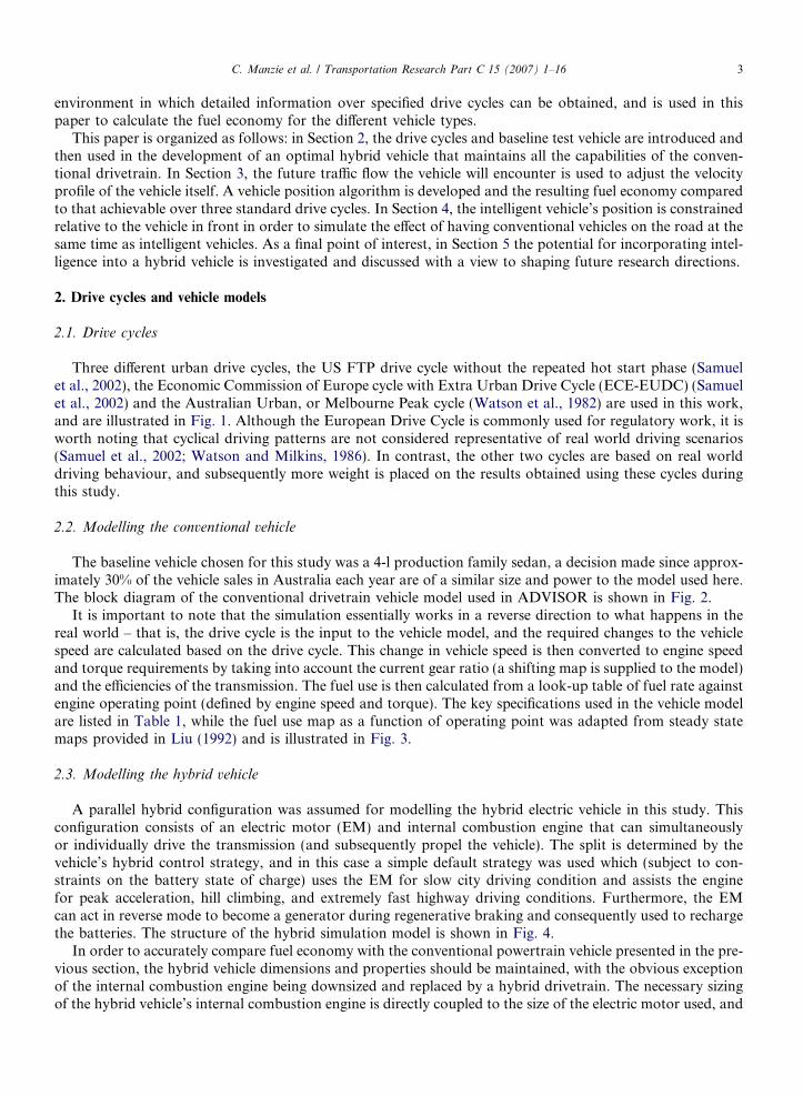
A parallel hybrid configuration was assumed for modelling the hybrid electric vehicle in this study. Thisconfiguration consists of an electric motor (EM) and internal combustion engine that can simultaneouslyor individually drive the transmission (and subsequently propel the vehicle). The split is determined by thevehicle’s hybrid control strategy, and in this case a simple default strategy was used which (subject to con-straints on the battery state of charge) uses the EM for slow city driving condition and assists the enginefor peak acceleration, hill climbing, and extremely fast highway driving conditions. Furthermore, the EMcan act in reverse mode to become a generator during regenerative braking and consequently used to rechargethe batteries. The structure of the hybrid simulation model is shown in Fig. 4.

In order to accurately compare fuel economy with the conventional powertrain vehicle presented in the pre-vious section, the hybrid vehicle dimensions and properties should be maintained, with the obvious exceptionof the internal combustion engine being downsized and replaced by a hybrid drivetrain. The necessary sizingof the hybrid vehicle’s internal combustion engine is directly coupled to the size of the electric motor used, and

Fig. 1. Australian urban (top) US FTP (middle) and ECE-EUDC (bottom) drive cycles.


hence an optimization process is required to ensure that the configuration is capable of meeting the perfor-mance requirements of the vehicle but in doing so uses the minimum amount of fuel. The performance require-ments of the conventional drivetrain were set as constraints on the optimization process and are listed in Table2. Another constraint during the optimization process is the change in state of battery charge at the beginning

Fig. 2. Block diagram of conventional drivetrain.

Table 1Conventional vehicle model specifications

Total weight 1642 kgChassis weight 1000 kgFrontal area 2.45 m2

Coefficient of Drag 0.366Vehicle weight distribution Front 55%, rear 45%Centre of mass height 0.5 mVehicle length 5.00 mTransmission Manual, 5 speedTransmission efficiency 95% (constant through all gears)Gear ratios 3.5:2.14:1.39:1:0.78Final drive ratio 2.92Gear changes 1! 2 and 2! 1 @ 24 km/h

2! 3 and 3! 2 @ 40 km/h3! 4 and 4! 3 @ 64 km/h4! 5 and 5! 4 @ 75 km/h

Tyre rolling radius 0.314 mTyre inertia 8.923 kg.m2

Tyre pressure, Tp 240 kPa

Fig. 3. Fuel consumption map of the test vehicle as a function of operating point.


and end of the cycle to prevent misleading fuel economy results arising from excessive use of the electric motor(which would then require battery replenishment and subsequently increased fuel use the next time the vehicleis run).

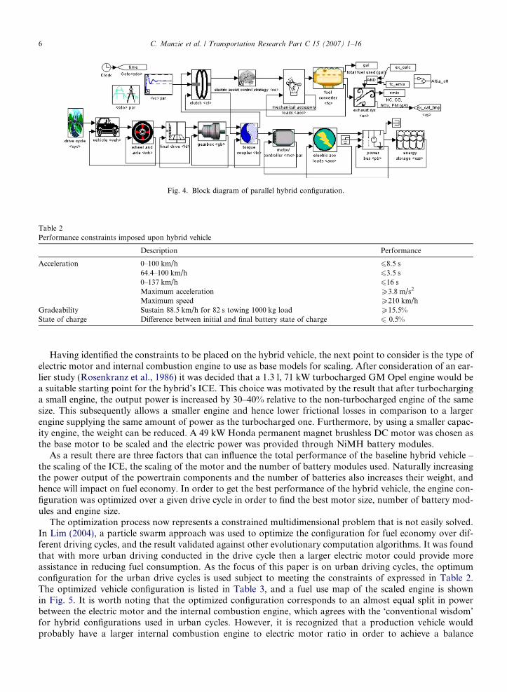
Fig. 4. Block diagram of parallel hybrid configuration.

Table 2Performance constraints imposed upon hybrid vehicle

Description Performance

Acceleration 0–100 km/h 68.5 s64.4–100 km/h 63.5 s0–137 km/h 616 sMaximum acceleration P3.8 m/s2

Maximum speed P210 km/hGradeability Sustain 88.5 km/h for 82 s towing 1000 kg load P15.5%State of charge Difference between initial and final battery state of charge 6 0.5%


Having identified the constraints to be placed on the hybrid vehicle, the next point to consider is the type ofelectric motor and internal combustion engine to use as base models for scaling. After consideration of an ear-lier study (Rosenkranz et al., 1986) it was decided that a 1.3 l, 71 kW turbocharged GM Opel engine would bea suitable starting point for the hybrid’s ICE. This choice was motivated by the result that after turbocharginga small engine, the output power is increased by 30–40% relative to the non-turbocharged engine of the samesize. This subsequently allows a smaller engine and hence lower frictional losses in comparison to a largerengine supplying the same amount of power as the turbocharged one. Furthermore, by using a smaller capac-ity engine, the weight can be reduced. A 49 kW Honda permanent magnet brushless DC motor was chosen asthe base motor to be scaled and the electric power was provided through NiMH battery modules.

As a result there are three factors that can influence the total performance of the baseline hybrid vehicle –the scaling of the ICE, the scaling of the motor and the number of battery modules used. Naturally increasingthe power output of the powertrain components and the number of batteries also increases their weight, andhence will impact on fuel economy. In order to get the best performance of the hybrid vehicle, the engine con-figuration was optimized over a given drive cycle in order to find the best motor size, number of battery mod-ules and engine size.

The optimization process now represents a constrained multidimensional problem that is not easily solved.In Lim (2004), a particle swarm approach was used to optimize the configuration for fuel economy over dif-ferent driving cycles, and the result validated against other evolutionary computation algorithms. It was foundthat with more urban driving conducted in the drive cycle then a larger electric motor could provide moreassistance in reducing fuel consumption. As the focus of this paper is on urban driving cycles, the optimumconfiguration for the urban drive cycles is used subject to meeting the constraints of expressed in Table 2.The optimized vehicle configuration is listed in Table 3, and a fuel use map of the scaled engine is shownin Fig. 5. It is worth noting that the optimized configuration corresponds to an almost equal split in powerbetween the electric motor and the internal combustion engine, which agrees with the ‘conventional wisdom’for hybrid configurations used in urban cycles. However, it is recognized that a production vehicle wouldprobably have a larger internal combustion engine to electric motor ratio in order to achieve a balance

Table 3Results of optimization for hybrid vehicle configuration

Internal combustion engine power (scaled from turbocharged 1.3 l, 71 kW engine) 66 kWElectric motor power (scaled from 49 kW Honda Permanent Magnet Brushless Motor) 68 kWNumber battery modules (D size 1.2 V NiMH 6 cells per module) 194

Fig. 5. Fuel consumption map of the turbocharged engine used in hybrid powertrain.

Table 4Fuel economies for conventional and optimized hybrid vehicles

Drive cycle Fuel economy (L/100 km) Improvement with hybrid (%)

Conventional drivetrain Hybrid drivetraina

Australian urban 11.9 10.1 15.3US FTP 10.8 8.2 24.7ECE-EUDC 10.6 8.5 19.8

a Change in battery state of charge constrained to <0.5%.


between urban and highway cycles. As a consequence, the real-world hybrid fuel economies would be lowerthan observed in this study.

Having obtained an optimized hybrid configuration, this vehicle was then simulated through all the urbandrive cycles with the restriction that the state of charge of the battery at the end of the drive cycle must bewithin 0.5% of the state of charge at the beginning. The results are provided in Table 4, and demonstratean average 20% fuel economy improvement across the drive cycles achieved through hybridization. However,these numbers must be qualified to some degree. Firstly, it is recalled that (in the interests of a fair comparisonwith a conventional drivetrain) the performance of the hybrid must satisfy the constraints given in Table 2. Arelaxation of part or all of these constraints will result in further improvements in the fuel economy of thehybrid vehicle, as would improvements in the vehicle’s coefficient of drag (both key parts of Toyota’s fueleconomy strategy for the Prius). Conversely, the concentration on urban drive cycles in the optimization pro-cedure results in an almost equal ratio between the electric motor and internal combustion engine power,which is unlikely to occur in production for a family sedan of this size. Despite these limitations, Table 4 doesallow a benchmark to be set against which the fuel economy of the intelligent vehicle can be measured.

3. The intelligent vehicle: a conventional drivetrain with telematics

One of the most significant contributors to fuel use in an urban environment is the stop start behaviour oftraffic flow. Through the use of telematics, a given vehicle can be made aware of the traffic and infrastructure


in which it is operating and adjust the driving condition en route. Communication between a fleet of vehicleshas been utilized in Automated Highway Systems previously (e.g. PATH) in order to improve the overallbehaviour of a platoon of vehicles in response to changing traffic conditions. Thus it is assumed for theintelligent vehicle in this paper that there exists a sensor network potentially incorporating inter-vehicle com-munication, radar and laser technologies that can be used to convey information about the surroundingtraffic. This traffic preview information can then be used to adjust the vehicle’s instantaneous velocity, whilstarriving at the destination at he same time as an un-equipped vehicle.

It is assumed that the output of the sensor network is assumed to be previewed traffic velocity information,vp(t), which is available up to Tp seconds ahead of the current time. This allows the position of a vehicle sub-jected to this traffic flow to be predicted based on its current position, x(t). The following algorithm outlineshow the intelligent vehicle may utilize the feedforward traffic information to adjust its own speed to minimizevehicle accelerations.

Intelligent Vehicle Velocity Modification (IVVM) Algorithm (unconstrained case)

Estimate vehicle position at time Tp in the future according to:

x̂ðt þ T pÞ ¼ xðtÞ þ aXT p=D

i¼1

vpðt þ iDÞD ð1Þ

where D is the sampling period (considered uniform) and a is a conversion constant. In order to reach thispredicted position with minimum stop–start behaviour the intelligent vehicle should attempt to use a con-stant speed, vint(t), calculated as follows:

vintðtÞ ¼x̂ðt þ T pÞ � xðtÞ

aT p

ð2Þ

This process, using Eqs. (1) and (2), is repeated every time new information becomes available. In the drivecycles used in this study, this period corresponds to once per second.

It is important to note that a critical assumption in this algorithm is that fuel use is linearly proportional toengine speed for a given torque requirement. Examination of the fuel use maps (shown in Figs. 3 and 5) indi-cates this is a reasonable assumption for relatively small changes in engine speed providing the current gear ismaintained. In the event that there was a highly non-linear relationship between fuel use and engine speed, itmay be necessary to consider engine-dependent strategies.

As an example of the alternative drive cycle, Fig. 6 demonstrates the difference if the unconstrained IVVMalgorithm is applied to the drive cycles with preview information about traffic flow from the next 50 s. Thiscorresponds to an average 450 metre distance over the US drive cycle, and could conceivably be achievedthrough on-board sensing and inter-vehicle communication only. While fuel economy minimization is themain outcome, there are further potential advantages to offset the cost of incorporating this technology intoa vehicle such as enhanced safety features including crash avoidance or protection, and improved safety atblind crossings (Tsugawa, 2002).

The amount of traffic preview information was varied from 0 to 180 s and the modified driving behaviourusing the vehicle velocity modification algorithm was then calculated for each of the US, Australian and ECE-EUDC cycles. While the traffic flow up to the preview time is simply assumed known in this study, it is highlylikely that a preview of three minutes would require information transfer between the infrastructure and thevehicle, and consequently greater telematic capability on-board the vehicle (and therefore higher overall vehi-cle cost). The fuel economy was then measured following simulation over the modified drive cycles and theresults are plotted as a function of preview time in Fig. 7. For comparison the fuel economy over the drivecycle if a hybrid vehicle without telematics capability also appears in the figure.

In all three cycles, quite significant improvements in fuel economy can be seen even for relatively short traf-fic previews. Interestingly, it shows that the improvement in fuel economy is much more marked for the twodrive cycles believed to better represent real world driving scenarios. Furthermore, there appears to be a ‘knee-point’ at approximately 50 s traffic preview beyond which the rate of improvement in fuel economy for extra

Fig. 6. Urban drive cycles (solid) and after use of 50 s traffic preview information (dotted).


preview information decreases. A quantitative comparison of several key statistics of these plots is presentedin Table 5. This data appears to reinforce that telematics realistically represents a more cost effective and

Fig. 7. Fuel economy as a function of preview information over different urban drive cycles. The fuel economies for the optimal hybridover the same drive cycles are also shown for comparison.

Table 5Quantitative comparison of fuel economy for varying degrees of feedforward traffic information

Drive cycle Fuel economy (L/100 km) Traffic preview for hybrid-equivalentfuel economy

Tp = 0 Tp = 50 % changea Tp = 180 % changea

Australian Urban 11.8 7.7 35 7.1 40 7US-FTP 10.8 8.4 22 7.8 28 60ECE-EUDC 10.6 9.2 13 8.6 19 182

a Change is calculated relative to no traffic preview (Tp = 0).


significant way of delivering improved fuel efficiencies in passenger vehicles. This notion is further strength-ened when it is recalled that the hybrid vehicle model used in this study is optimized for urban driving witha near equal split in the power capability of the internal combustion engine and the electric motor. A furtherfuel economy benefit of incorporating telematics not accounted for here may be achievable through closerinter-vehicle spacing made possible by automated highway systems resulting in a reduced coefficient of dragfor each vehicle (other than the lead vehicle in the platoon). In Barth (2000), the improvements in fuel econ-omy solely through reduced drag coefficients inherent in a platooning situation were estimated to be in therange 5–15% over highway cycles.

However, there are some limitations of this study so far in assessing the performance of the intelligent vehi-cles. Thus far, it has been considered that the intelligent vehicle can adapt its driving behaviour without regardto any other conditions. This assumption neglects conditions enforced by both the infrastructure and other‘un-intelligent’ vehicles on the road. Hence in the next section, the allowable intelligent vehicle speed willbe constrained to enforce conditions imposed by the surrounding traffic, and the subsequent effects on the fueleconomy over the same urban drive cycles assessed.

4. Implication of restricting relative position of the intelligent vehicle

While significant improvements in fuel economy through the use of feedforward information about trafficconditions supplied by a sensor network were observed in the previous section, it is unlikely that there wouldbe a quantum shift to this technology by all road users. To gauge the impact of the technology using low levelsof consumer uptake, it is necessary to remove the assumption that the intelligent vehicle’s velocity (and posi-tion) can be assigned irrespective of the traffic flow in which it operates. For example, the adapted velocityprofiles obtained using the velocity modification algorithm of the previous section demonstrate a phase lead


at certain points in time (for example the first 20 s of all the drive cycles in Fig. 6). This indicates the intelligentvehicle starts moving before it would have if no preview information were available.

Naturally, there will be some cases whereby this situation is not feasible, one example is a traffic signalenforcing vehicle stationarity, and hence it is important to reflect this by applying constraints to the velocityalgorithm. The constraint applied in this section is that the intelligent vehicle cannot overtake the position itwould occupy on the road if it were traveling without any preview information, i.e. it cannot overtake theun-intelligent vehicle position, or equivalently an unintelligent vehicle directly in front of the intelligent vehicleand traveling at a velocity indicated by the drive cycle. This constraint has been enforced by adjusting the intel-ligent vehicle’s velocity determination algorithm described in the previous section to the one described below.

Intelligent Vehicle Velocity Modification Algorithm (overtaking disallowed)

Step 1: Find position trajectory of the vehicle in front of (leading) the intelligent vehicle over the previewduration, i.e.

x̂leadðt þ iDÞ ¼ xleadðtÞ þ aXi

k¼0

vleadðt þ iDÞD for i ¼ 1; . . . ;T p

Dð3Þ

Note that the sampling period D is assumed constant, but Eq. (3) is readily adapted to non-uniformsampling.

Step 2: Set iteration number, j to zero.Step 3: Find the candidate constant velocity over the next Tp � j seconds, such that the positions of the intel-

ligent and leading vehicle are equal, i.e. x̂intðt þ T p � jDÞ ¼ x̂leadðt þ T p � jDÞ. This candidate velocityis calculated according to:

�vjint ¼

x̂leadðt þ T p � jDÞ � xintðtÞaðT p � jDÞ ð4Þ

Step 4: Develop a trajectory for the intelligent vehicle based on �vjint over the interval from the current time to

Tp � jD, i.e.

x̂intðt þ iDÞ ¼ xintðtÞ þ iDa�vjint for iD ¼ D; . . . ; T p � jD ð5Þ

Step 5: Test whether the predicted intelligent vehicle trajectory overtakes the predicted ‘lead’ vehicle trajec-tory, and if necessary update the candidate constant velocity to avoid overtaking, i.e.• If x̂leadðt þ iDÞ > x̂intðt þ iDÞfor iD ¼ D; . . . ; T p � jD then use �vj

int as the intelligent vehicle’s velocity attime t.

• Otherwise, if x̂leadðt þ iDÞ 6 x̂intðt þ iDÞ for at least one value of iD, then increment j and return toStep 3.

The position trajectories calculated for an un-intelligent vehicle, an intelligent vehicle with velocity modifiedaccording to the first algorithm (which allows overtaking) and for the new algorithm (which prevents overtak-ing) are illustrated over a section of a drive cycle in Fig. 8. It is clear that when the lead vehicle is stationary(between 6 and 19 s), the constrained solution results in a slower velocity over the period up to 20 s to ensurethat the no-overtaking constraint is not violated. In Fig. 9, the full Australian urban drive cycle is subjected tomodified algorithm.

In Fig. 10, the position relative to the lead vehicle is compared over the entire Australian Urban drive cyclefor each of the two proposed algorithms. From this figure, it is clear that the maximum separation occurswhen the vehicle speeds are highest, and that by preventing overtaking the maximum distance between anintelligent and un-intelligent vehicle is close to 400 m. In Fig. 11, the average and maximum gaps betweenan intelligent and un-intelligent vehicle are plotted as a function of preview information for each of the threedrive cycles used in this study. It can be seen that the unconstrained intelligent vehicle would (on average) tendto lead the un-intelligent vehicle. Preventing overtaking would result in an average separation that growsmonotonically with traffic preview. The maximum separation between an intelligent and unintelligent vehicleis also seen to grow monotonically with traffic preview. While the benefits of improved fuel economy alsoincrease, the consumer acceptance of (or resistance to) increasingly large gaps in the traffic flow is likely to

Fig. 8. Position projections for the lead vehicle and the intelligent vehicle with overtaking of the lead vehicle allowed and disallowed. Atraffic preview of 25 s has been used in both intelligent vehicle algorithms.

Fig. 9. Australian urban velocity profile (solid) and modified using a traffic preview of 50 s while preventing overtaking (dotted).


limit the effectiveness of extended traffic previews. It would be relatively straightforward to limit the maximumdistance between vehicles by imposing a further constraint in the IVVM algorithm, although this would resultin some deterioration in achievable fuel economy.

In Fig. 12, the effect on fuel economy of preventing overtaking is assessed for each of the three drive cycles.It is observed that there is only small degradation in performance for the most part, although the achievablemodifications under an EUDC-ECE type traffic flow is limited by preventing overtaking and subsequently nofurther improvement is observed for traffic previews above 80 s. Thus Figs. 11 and 12 present a (not unex-pected) conflict – as fuel economy improves, the maximum gap between an intelligent vehicle and an unintel-ligent vehicle increases thereby testing driver acceptance.

5. Hybrid vehicle equipped with telematics

As a final point of interest, rather than contrasting the performance that can be achieved through the twodifferent technologies, this section deals with the achievable fuel economies if the technologies are combined to

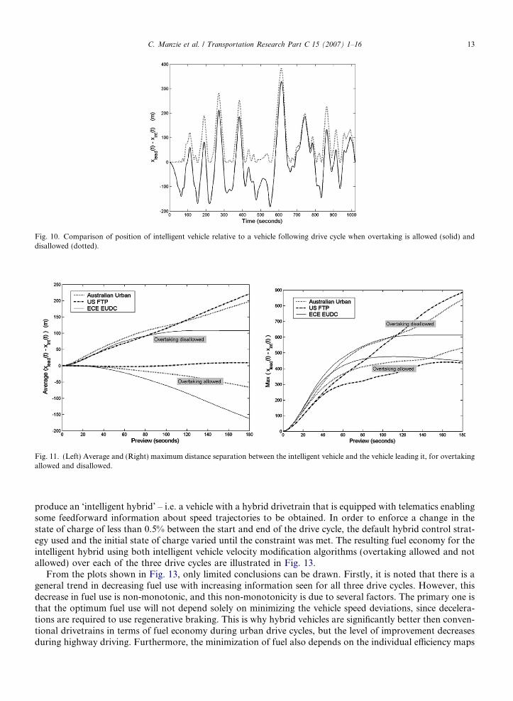
Fig. 10. Comparison of position of intelligent vehicle relative to a vehicle following drive cycle when overtaking is allowed (solid) anddisallowed (dotted).

Fig. 11. (Left) Average and (Right) maximum distance separation between the intelligent vehicle and the vehicle leading it, for overtakingallowed and disallowed.


produce an ‘intelligent hybrid’ – i.e. a vehicle with a hybrid drivetrain that is equipped with telematics enablingsome feedforward information about speed trajectories to be obtained. In order to enforce a change in thestate of charge of less than 0.5% between the start and end of the drive cycle, the default hybrid control strat-egy used and the initial state of charge varied until the constraint was met. The resulting fuel economy for theintelligent hybrid using both intelligent vehicle velocity modification algorithms (overtaking allowed and notallowed) over each of the three drive cycles are illustrated in Fig. 13.

From the plots shown in Fig. 13, only limited conclusions can be drawn. Firstly, it is noted that there is ageneral trend in decreasing fuel use with increasing information seen for all three drive cycles. However, thisdecrease in fuel use is non-monotonic, and this non-monotonicity is due to several factors. The primary one isthat the optimum fuel use will not depend solely on minimizing the vehicle speed deviations, since decelera-tions are required to use regenerative braking. This is why hybrid vehicles are significantly better then conven-tional drivetrains in terms of fuel economy during urban drive cycles, but the level of improvement decreasesduring highway driving. Furthermore, the minimization of fuel also depends on the individual efficiency maps

Fig. 12. Fuel economy as a function of preview information with overtaking allowed and disallowed using the Australian urban cycle (topleft) US FTP cycle (top right) and ECE-EUDC cycle (bottom). For reference optimized hybrid fuel economy is also included in each plot.


of the internal combustion engine and electric motor, as well as the switching strategy of the hybrid controller.A dynamic programming optimization approach over an entire drive cycle has been used to derive the optimalswitching strategy when the vehicle speed is fixed to the drive cycle in Kirschbaum et al. (2002), however the

Fig. 13. Fuel economy of intelligent hybrid vehicle as a function of preview time.


optimal use of limited traffic preview information in an online controller remains an open problem, particu-larly if vehicle speed is allowed to vary away from the traffic flow. If a variable vehicle velocity is added as adimension to the constrained problem the solution is certainly non-trivial and requires further research effort.


6. Conclusions

This paper presents a comparison between two of the emerging technologies in automotive systems, hybriddrivetrains and telematics capability. Following the development of an optimal hybrid configuration thatmatches the performance of the baseline test vehicle, it was found through simulation that the fuel economyimprovements possible through optimal hybridization ranged between 15% and 25% relative to the baselinevehicle over three standard urban drive cycles.

The test vehicle was then equipped with telematic capability, and an algorithm proposed that made use ofpreview information provided by the telematics to determining the vehicle’s modified speed at each point ofthe drive-cycle. It was observed that the same fuel economy as recorded for the hybrid drive cycle could beachieved with less than 60 s preview information on two realistic drive cycles. Further traffic flow informationup to 180 s resulted in as much as 33% fuel economy improvements relative to the original test vehicle.

The proposed algorithm was then constrained to prevent overtaking of any part of the traffic flow. It wasfound that the fuel economy was only slightly worse than for the unconstrained case, and again matched thehybrid fuel economy with relatively short preview information. The potential gaps in traffic that would resultfrom the use of both proposed algorithms was also investigated. This highlighted the trade-off between inter-mittent positional gaps to an un-intelligent car immediately in front of the intelligent vehicle and fuel economyimprovement.

Finally, the two technologies (hybrid and telematics) were combined in one vehicle to create an ‘intelligenthybrid’ vehicle. While there were general trends indicating improvement in fuel economy with traffic preview,the multi-dimensional nature of the problem (current vehicle speed, power split between the electric motor andinternal combustion engine and battery state of charge must all be considered) ensures that the optimal use ofthe feedforward information, particularly for short traffic previews, remains an ongoing research problem.

References

Barth, M., 2000. An emissions and energy comparison between a simulated automated highway system and current traffic conditions.Intelligent Transportation Systems, IEEE, 358–363.

Durrant-Whyte, H.F., Rao, B.Y.S., Hu, H., 1990. Toward a fully decentralized architecture for multi-sensor data fusion. In: Proceedingsof the 1990 IEEE International Conference on Robotics and Automation, vol. 2, pp. 1331–1336.

Kirschbaum, F., Back, M., Hart, M., 2002. Determination of the fuel-optimal trajectory along a known route. In: IFAC 15th TriennialWorld CongressBarcelona, Spain.

Levinson, D., 2003. The value of advanced traveler information systems for route choice. Transportation Research Part C: EmergingTechnologies 11, 75–87.

Lim, K., 2004. Modelling and Optimisation of Hybrid Electric Vehicles. Masters Dissertation in Department of Mechanical andManufacturing Engineering.

Liu, Y., 1992. Strategies for Improving Vehicle Energy Efficiency. PhD Dissertation in Department of Mechanical and ManufacturingEngineering, The University of Melbourne.

Rajamani, R., Tan, H.-S., Law, B.K., Zhang, W.-B., 2000. Demonstration of Integrated Longitudinal and Lateral Control for theOperation of Automated Vehicles in Platoons. IEEE Transactions on Control Systems Technology 8, 695–708.

Rosenkranz, H.G., Watson, H.C., Bryce, W., Lewis, A., 1986. Driveability, fuel consumption and emissions of a 1.3 l turbocharged sparkignition engine developed as replacement for a 2.0 l naturally aspirated engine. Proceeding of the Institution of Mechanical Engineers,139–150.

Samuel, S., Austin, L., Morrey, D., 2002. Automotive test drive cycles for emissions measurement and real-world emission levels – areview. Proceedings of the Institution of Mechanical Engineers 216, 555–564.

Swaroop, D., Hedrick, J.K., 1996. String stability of interconnected systems. IEEE Transactions on Automatic Control 41, 349–357.Tomizuka, M., 1994. Advanced vehicle control systems (AVCS) research for automated highway systems in California PATH. In:

Proceedings of the Vehicle Navigation and Information Systems Conference, pp. PLEN41–PLEN45.Tsugawa, S., 2002. Inter-vehicle communications and their applications to intelligent vehicles: an overviewIntelligent Vehicle Symposium

2002, Vol. 2. IEEE, pp. 564–569.Watson, H.C., Milkins, E.E., 1986. An International Drive Cycle. Paper 865042, 21st FISITA Congress Belgrade, pp. 405–414.Watson, H.C., Milkins, E.E., Braunsteins, J., 1982. The development of the Melbourne peak cycle. In: Proceedings of the Joint SAE-A/

ARRB Second Conference on Traffic, Energy and Emissions, Melbourne, Australia.Wipke, K., Cuddy, M., Burch, S., 1999. ADVISOR 2.1: A User Friendly Advanced Powertrain Simulation Using a Combined Backward/

Forward Approach. IEEE Transactions on Vehicular Technology 48, 1751–1761.

Documents

Fuel economy improvements for urban driving: Hybrid vs. intelligent