Embed Size (px)
Citation preview

Frontiers of Statistical Decision Making and Bayesian Analysis
1
Frontiers of Statistical Decision Making and Bayesian Analysis
1
Introduction to Spatial Data and Models
Sudipto Banerjee1 and Andrew O. Finley2
1 Biostatistics, School of Public Health, University of Minnesota, Minneapolis, Minnesota, U.S.A.
2 Department of Forestry & Department of Geography, Michigan State University, Lansing Michigan, U.S.A.
March 3, 2010
1
Introduction to spatial data and models
Researchers in diverse areas such as climatology, ecology,environmental health, and real estate marketing areincreasingly faced with the task of analyzing data that are:
highly multivariate, with many important predictors andresponse variables,
geographically referenced, and often presented as maps,and
temporally correlated, as in longitudinal or other time seriesstructures.
⇒ motivates hierarchical modeling and data analysis forcomplex spatial (and spatiotemporal) data sets.
2 Frontiers of Statistical Decision Making and Bayesian Analysis

Frontiers of Statistical Decision Making and Bayesian Analysis
2
Frontiers of Statistical Decision Making and Bayesian Analysis
2
Introduction to spatial data and models Type of spatial data
point-referenced data, where Y (s) is a random vector at alocation s ∈ <r, where s varies continuously over D, afixed subset of <r that contains an r-dimensional rectangleof positive volume;
areal data, where D is again a fixed subset (of regular orirregular shape), but now partitioned into a finite number ofareal units with well-defined boundaries;
point pattern data, where now D is itself random; its indexset gives the locations of random events that are thespatial point pattern. Y (s) itself can simply equal 1 for alls ∈ D (indicating occurrence of the event), or possibly givesome additional covariate information (producing a markedpoint pattern process).
3 Frontiers of Statistical Decision Making and Bayesian Analysis
Introduction to spatial data and models Exploration of spatial data
First step in analyzing data
First Law of Geography: Mean + Error
Mean: first-order behavior
Error: second-order behavior (covariance function)
EDA tools examine both first and second order behavior
Preliminary displays: Simple locations to surface displays
4 Frontiers of Statistical Decision Making and Bayesian Analysis

Frontiers of Statistical Decision Making and Bayesian Analysis
3
Frontiers of Statistical Decision Making and Bayesian Analysis
3
Introduction to spatial data and models Exploration of spatial data
First step in analyzing data
First Law of Geography: Mean + Error
Mean: first-order behavior
Error: second-order behavior (covariance function)
EDA tools examine both first and second order behavior
Preliminary displays: Simple locations to surface displays
4 Frontiers of Statistical Decision Making and Bayesian Analysis
Introduction to spatial data and models Exploration of spatial data
First Law of Geography
data mean
=
error
+
5 Frontiers of Statistical Decision Making and Bayesian Analysis
Introduction to spatial data and models Exploration of spatial data
Scallops Sites
•
••
••
•
••
•
•
••••
•
•
••
••
••••
••
•
•
•
••
• ••
••
•• •
•
•
• •
•• •
•
•••
•
•
••••
••
• •
•••• •
••
••
•••
••
••• •••
••••••
•
••
••
•
•••
•••
•
• ••••
•
••
• ••
• ••
••
•••
••
••• •
•• •
• •••••
••
•
•••
• ••• •
••• •
6 Frontiers of Statistical Decision Making and Bayesian Analysis
Introduction to spatial data and models Deterministic surface interpolation
Spatial surface observed at finite set of locationsS = s1, s2, ..., snTessellate the spatial domain (usually with data locationsas vertices)Fit an interpolating polynomial:
f(s) =∑i
wi(S ; s)f(si)
“Interpolate” by reading off f(s0).Issues:
Sensitivity to tessellationsChoices of multivariate interpolatorsNumerical error analysis
7 Frontiers of Statistical Decision Making and Bayesian Analysis

Frontiers of Statistical Decision Making and Bayesian Analysis
4
Frontiers of Statistical Decision Making and Bayesian Analysis
4
Introduction to spatial data and models Scallops data: image and contour plots
−73.5 −73.0 −72.5 −72.0
39.0
39.5
40.0
40.5
Longitude
Latit
ude
8 Frontiers of Statistical Decision Making and Bayesian Analysis
Introduction to spatial data and models Scallops data: image and contour plots
Drop-line scatter plot
9 Frontiers of Statistical Decision Making and Bayesian Analysis
Introduction to spatial data and models Scallops data: image and contour plots
Surface plot
-121.36-121.34
-121.32-121.3
-121.28
Longitude
37.96
37.98
38
38.02
38.04
Latitude
1111
.211
.411
.611
.812
12.2
12.4
logS
P
10 Frontiers of Statistical Decision Making and Bayesian Analysis
Introduction to spatial data and models Scallops data: image and contour plots
Image contour plot
−121.36 −121.34 −121.32 −121.30 −121.28 −121.26
37.9
637
.98
38.0
038
.02
38.0
4
Longitude
Latit
ude
11 Frontiers of Statistical Decision Making and Bayesian Analysis
Introduction to spatial data and models Scallops data: image and contour plots
Locations form patterns
•
••
•
•
•
••
•
•
•
•
•
•
•
••
• •
•
•
•
••
•
•
•
• •
•
•
•
•
•
•
•
••
•
•
•
•
•
•
••
••
•
•
••••
•
••
•
•
•
••
•
•
• •
•
•••
•
•
•
•
•
•
•
•
•
•
••
•
•
•
•
•
•
•
••
••
•
•
•
•
••
•
••
•
•
•
•
•
•
••
•
• •
•
•
•
• •
••
•
•
•
• ••
•
•
•
•
•
•
•
•
•
•
•
•
•
•
•
••
•
•
•
•
•
••
••
•
•
•
••
•
•
•
•
••
••
•
•
•
•
•
•
•
•
•
•
•
•
••
•
•
•
•
•
•
•
•
•
•
••
•
••
•
•
•
•
•
•
•
••
•
•
•
••
•
•
•
•
•
•
•
•
•
•
•
•
•
•
•
•
•
•
•
•
••
••
• •
•
•• •
•
•
•
•
••
•
•
•
•
•
•
•
••
•
•
•
•
•
•
•
•
•
•
•
•
•••
•
•
•
•
•
•
••
••
•
•
••
•
•
•
•
•
•
•
•
••
•
•
••
••
•
•
•
•
•
•
••
•
•
•
•
•
••
••
•
•
••
• •
•
••
•
••
••
•
•
•
•
••
• •
••
•
•
•
•
•
•
•
•
•
••
•
•
•
•
•
•
•
•
•
•
•
•
•
•
••
•
•
•
•
•
•
•
•
•
•
•
•
•
••
••
•
•
•
•
••
•• •
•
•
•
•
•
••
•
•
•
• •
•
•
•
•
•
•• ••
•
•
•
•
••
•
•
•
•••
•
•
•
•
•
•
•
•
•
•
•
••
•
•
•
•
•
•
•
•
••
•
•
•
•
••
•
•
•
•
•
•
•
•
•
••
•
•
•
•
•
••
•
•
••
•
• •
•
••
•
•
•••
• ••
•
•
•
•
•
•
•
•
••
•
•
•
•
•
•
••
••
•
•
•
••
••
•
••
••
•
•
•
•
•
•
•
•
•
•
•
•• •
•
•
•
•
•
•• • •
•
•
•
•
•
•
•
••
•
•
•
•
•
•
•
•••
•
• •
•
••
•
•
•
•
•
•
•
••
•
•
•
•
•
••
••
•
•
•
•
•
•
•
•
••
•
•
•
•
•
•
•
•
•
•
•
•
•
•
•
• •
•
•
•
•
•
•
•
•
•
•
• ••
•
•
•
•
•
•
•
•
•
•
•
••
•
•
•
•
•
•
• •••
•
•
•
•
•
•
•
•
•
•
••
•
•
•
•
•
•
• •
•
•
•
•
•
•
• • •
•
• ••
•
•
•
••
••
•
•
••
•
•
•
•
•
•
•
•
•
•
•
•
•
•
•
•
•
•
•
•
•
•
••
•
•
•
•
•
•
•
•
••
•••
•
•
•
•
•
•
•
•
•
••
•
••
•
•
•
••
•
•
•
•
••
•
••
•
••
•
••
•
•
•
•
•
•
•
•
•
•
•
•
•
•
••
•
•
•
••
•
•
••
•
•
•
•
•
•
•
•
••
•
••
•
•
•
•
•
•
•
•
•
•
•
•
•
•
•
•
•
•
•• •
•
••
•
•
•
•
•
•
•
•
•
•
•
•
•
•
•
••
•
•
•
••
• •
•
•
•
•
•
•
•
•
•
•
•
•
••
•
•
••
•
•
•
•
•• •
•
•
•
•
•
•
••
•
•
•
•
•
•
•••
•
••
•
• •
•
•
•
••
•
•
•
•
•
•
•
•
•
•
• • •
•
•
•
•
•
••
• •
•
•
•
•
•
•
•
•
•
•
•
•
••
•
•
•
•
•
•
•
•
••
••
•
•
• •
•
•
•
••
••
•
•
•
•
•
•
•
••
•
•
•
•
•
•
•
•
••
•
•
•
•
••
•
•
••
•
••
•
••
•
•
•
•
•
•
•
•
•
•
•
•
•
•
• •
•
•
•
•
••
•
••
•
•
••
•
•
•
•
••
•
•
•
•
•
•
•
• •
•
••
•
•
•
•
••
•••
•
••
•
•
•
•
•
•
•
•
•
•
••
•
•
•
•
• •
••
•
•
•
•
•
•
•
•
•
••
•
•
•
• •
••
• •
• •
•
•
• •
•
•
•
•
•
•
•
••
•
••
•
•• •
•
•
•
•
•
•
•
•
128100 128150 128200 128250 128300
1031
350
1031
400
1031
450
1031
500
1031
550
Eastings
Nor
thin
gs
128100 128150 128200 128250 128300
1031
350
1031
400
1031
450
1031
500
1031
550
12 Frontiers of Statistical Decision Making and Bayesian Analysis
Introduction to spatial data and models Scallops data: image and contour plots
Surface features
128100128150
128200128250
128300
Eastings
1031350
1031400
1031450
1031500
1031550
Northings
02
46
810
1214
Shr
ub D
ensi
ty
13 Frontiers of Statistical Decision Making and Bayesian Analysis

Frontiers of Statistical Decision Making and Bayesian Analysis
5
Frontiers of Statistical Decision Making and Bayesian Analysis
5
Introduction to spatial data and models Scallops data: image and contour plots
Interesting plot arrangements
456300 456320 456340 456360 456380 456400 456420 456440
4879
050
4879
100
4879
150
4879
200
456300 456320 456340 456360 456380 456400 456420 456440
4879
050
4879
100
4879
150
4879
200
E−W UTM coordinates
N−
S U
TM
coo
rdin
ates
14 Frontiers of Statistical Decision Making and Bayesian Analysis
Introduction to spatial data and models Elements of point-level modelling
Point-level modelling refers to modelling of spatialdatacollected at locations referenced by coordinates (e.g.,lat-long, Easting-Northing).
Fundamental concept: Data from a spatial processY (s) : s ∈ D, where D is a fixed subset in Euclideanspace.Example: Y (s) is a pollutant level at site s
Conceptually: Pollutant level exists at all possible sitesPractically: Data will be a partial realization of a spatialprocess – observed at s1, . . . , snStatistical objectives: Inference about the process Y (s);predict at new locations.
15 Frontiers of Statistical Decision Making and Bayesian Analysis
Introduction to spatial data and models Elements of point-level modelling
Point-level modelling refers to modelling of spatialdatacollected at locations referenced by coordinates (e.g.,lat-long, Easting-Northing).Fundamental concept: Data from a spatial processY (s) : s ∈ D, where D is a fixed subset in Euclideanspace.
Example: Y (s) is a pollutant level at site s
Conceptually: Pollutant level exists at all possible sitesPractically: Data will be a partial realization of a spatialprocess – observed at s1, . . . , snStatistical objectives: Inference about the process Y (s);predict at new locations.
15 Frontiers of Statistical Decision Making and Bayesian Analysis
Introduction to spatial data and models Elements of point-level modelling
Point-level modelling refers to modelling of spatialdatacollected at locations referenced by coordinates (e.g.,lat-long, Easting-Northing).Fundamental concept: Data from a spatial processY (s) : s ∈ D, where D is a fixed subset in Euclideanspace.Example: Y (s) is a pollutant level at site s
Conceptually: Pollutant level exists at all possible sites
Practically: Data will be a partial realization of a spatialprocess – observed at s1, . . . , snStatistical objectives: Inference about the process Y (s);predict at new locations.
15 Frontiers of Statistical Decision Making and Bayesian Analysis
Introduction to spatial data and models Elements of point-level modelling
Point-level modelling refers to modelling of spatialdatacollected at locations referenced by coordinates (e.g.,lat-long, Easting-Northing).Fundamental concept: Data from a spatial processY (s) : s ∈ D, where D is a fixed subset in Euclideanspace.Example: Y (s) is a pollutant level at site s
Conceptually: Pollutant level exists at all possible sitesPractically: Data will be a partial realization of a spatialprocess – observed at s1, . . . , sn
Statistical objectives: Inference about the process Y (s);predict at new locations.
15 Frontiers of Statistical Decision Making and Bayesian Analysis

Frontiers of Statistical Decision Making and Bayesian Analysis
6
Frontiers of Statistical Decision Making and Bayesian Analysis
6
Introduction to spatial data and models Elements of point-level modelling
Point-level modelling refers to modelling of spatialdatacollected at locations referenced by coordinates (e.g.,lat-long, Easting-Northing).Fundamental concept: Data from a spatial processY (s) : s ∈ D, where D is a fixed subset in Euclideanspace.Example: Y (s) is a pollutant level at site s
Conceptually: Pollutant level exists at all possible sitesPractically: Data will be a partial realization of a spatialprocess – observed at s1, . . . , snStatistical objectives: Inference about the process Y (s);predict at new locations.
15 Frontiers of Statistical Decision Making and Bayesian Analysis
Introduction to spatial data and models Stationary Gaussian processes
Suppose our spatial process has a mean, µ (s) = E (Y (s)),and that the variance of Y (s) exists for all s ∈ D.
Strong stationarity: If for any given set of sites, and anydisplacement h, the distribution of (Y (s1), ..., Y (sn)) is thesame as, (Y (s1 + h), ..., Y (sn + h)).Weak stationarity: Constant mean µ(s) = µ, andCov(Y (s), Y (s + h)) = C(h): the covariance depends onlyupon the displacement (or separation) vector.Strong stationarity implies weak stationarityThe process isGaussian if Y = (Y (s1), . . . , Y (sn)) has amultivariate normal distribution.For Gaussian processes, strong and weak stationarity areequivalent.
16 Frontiers of Statistical Decision Making and Bayesian Analysis
Introduction to spatial data and models Stationary Gaussian processes
Suppose our spatial process has a mean, µ (s) = E (Y (s)),and that the variance of Y (s) exists for all s ∈ D.
Strong stationarity: If for any given set of sites, and anydisplacement h, the distribution of (Y (s1), ..., Y (sn)) is thesame as, (Y (s1 + h), ..., Y (sn + h)).Weak stationarity: Constant mean µ(s) = µ, andCov(Y (s), Y (s + h)) = C(h): the covariance depends onlyupon the displacement (or separation) vector.
Strong stationarity implies weak stationarityThe process isGaussian if Y = (Y (s1), . . . , Y (sn)) has amultivariate normal distribution.For Gaussian processes, strong and weak stationarity areequivalent.
16 Frontiers of Statistical Decision Making and Bayesian Analysis
Introduction to spatial data and models Stationary Gaussian processes
Suppose our spatial process has a mean, µ (s) = E (Y (s)),and that the variance of Y (s) exists for all s ∈ D.
Strong stationarity: If for any given set of sites, and anydisplacement h, the distribution of (Y (s1), ..., Y (sn)) is thesame as, (Y (s1 + h), ..., Y (sn + h)).Weak stationarity: Constant mean µ(s) = µ, andCov(Y (s), Y (s + h)) = C(h): the covariance depends onlyupon the displacement (or separation) vector.Strong stationarity implies weak stationarity
The process isGaussian if Y = (Y (s1), . . . , Y (sn)) has amultivariate normal distribution.For Gaussian processes, strong and weak stationarity areequivalent.
16 Frontiers of Statistical Decision Making and Bayesian Analysis
Introduction to spatial data and models Stationary Gaussian processes
Suppose our spatial process has a mean, µ (s) = E (Y (s)),and that the variance of Y (s) exists for all s ∈ D.
Strong stationarity: If for any given set of sites, and anydisplacement h, the distribution of (Y (s1), ..., Y (sn)) is thesame as, (Y (s1 + h), ..., Y (sn + h)).Weak stationarity: Constant mean µ(s) = µ, andCov(Y (s), Y (s + h)) = C(h): the covariance depends onlyupon the displacement (or separation) vector.Strong stationarity implies weak stationarityThe process isGaussian if Y = (Y (s1), . . . , Y (sn)) has amultivariate normal distribution.
For Gaussian processes, strong and weak stationarity areequivalent.
16 Frontiers of Statistical Decision Making and Bayesian Analysis
Introduction to spatial data and models Stationary Gaussian processes
Suppose our spatial process has a mean, µ (s) = E (Y (s)),and that the variance of Y (s) exists for all s ∈ D.
Strong stationarity: If for any given set of sites, and anydisplacement h, the distribution of (Y (s1), ..., Y (sn)) is thesame as, (Y (s1 + h), ..., Y (sn + h)).Weak stationarity: Constant mean µ(s) = µ, andCov(Y (s), Y (s + h)) = C(h): the covariance depends onlyupon the displacement (or separation) vector.Strong stationarity implies weak stationarityThe process isGaussian if Y = (Y (s1), . . . , Y (sn)) has amultivariate normal distribution.For Gaussian processes, strong and weak stationarity areequivalent.
16 Frontiers of Statistical Decision Making and Bayesian Analysis

Frontiers of Statistical Decision Making and Bayesian Analysis
7
Frontiers of Statistical Decision Making and Bayesian Analysis
7
Introduction to spatial data and models Stationary Gaussian processes
Variograms
Suppose we assume E[Y (s + h)− Y (s)] = 0 and define
E[Y (s + h)− Y (s)]2 = V ar (Y (s + h)− Y (s)) = 2γ (h) .
This is sensible if the left hand side depends only upon h.Then we say the process is intrinsically stationary.
γ(h) is called the semivariogram and 2γ(h) is called thevariogram.
Note that intrinsic stationarity defines only the first and secondmoments of the differences Y (s + h)− Y (s). It says nothingabout the joint distribution of a collection of variablesY (s1), . . . , Y (sn), and thus provides no likelihood.
17 Frontiers of Statistical Decision Making and Bayesian Analysis
Introduction to spatial data and models Stationary Gaussian processes
Variograms
Suppose we assume E[Y (s + h)− Y (s)] = 0 and define
E[Y (s + h)− Y (s)]2 = V ar (Y (s + h)− Y (s)) = 2γ (h) .
This is sensible if the left hand side depends only upon h.Then we say the process is intrinsically stationary.γ(h) is called the semivariogram and 2γ(h) is called thevariogram.
Note that intrinsic stationarity defines only the first and secondmoments of the differences Y (s + h)− Y (s). It says nothingabout the joint distribution of a collection of variablesY (s1), . . . , Y (sn), and thus provides no likelihood.
17 Frontiers of Statistical Decision Making and Bayesian Analysis
Introduction to spatial data and models Stationary Gaussian processes
Intrinsic Stationarity and Ergodicity
Relationship between γ(h) and C(h):
2γ(h) = V ar(Y (s + h)) + V ar(Y (s))− 2Cov(Y (s + h), Y (s))= C(0) + C(0)− 2C(h)= 2[C(0)− C(h)].
Easy to recover γ from C. The converse needs theadditional assumption of ergodicity: lim‖u‖→∞C(u) = 0.So lim‖u‖→∞ γ(u) = C(0), and we can recover C from γ aslong as this limit exists.
C(h) = lim‖u‖→∞
γ(u)− γ(h).
18 Frontiers of Statistical Decision Making and Bayesian Analysis
Introduction to spatial data and models Stationary Gaussian processes
Intrinsic Stationarity and Ergodicity
Relationship between γ(h) and C(h):
2γ(h) = V ar(Y (s + h)) + V ar(Y (s))− 2Cov(Y (s + h), Y (s))= C(0) + C(0)− 2C(h)= 2[C(0)− C(h)].
Easy to recover γ from C. The converse needs theadditional assumption of ergodicity: lim‖u‖→∞C(u) = 0.
So lim‖u‖→∞ γ(u) = C(0), and we can recover C from γ aslong as this limit exists.
C(h) = lim‖u‖→∞
γ(u)− γ(h).
18 Frontiers of Statistical Decision Making and Bayesian Analysis
Introduction to spatial data and models Stationary Gaussian processes
Intrinsic Stationarity and Ergodicity
Relationship between γ(h) and C(h):
2γ(h) = V ar(Y (s + h)) + V ar(Y (s))− 2Cov(Y (s + h), Y (s))= C(0) + C(0)− 2C(h)= 2[C(0)− C(h)].
Easy to recover γ from C. The converse needs theadditional assumption of ergodicity: lim‖u‖→∞C(u) = 0.So lim‖u‖→∞ γ(u) = C(0), and we can recover C from γ aslong as this limit exists.
C(h) = lim‖u‖→∞
γ(u)− γ(h).
18 Frontiers of Statistical Decision Making and Bayesian Analysis

Frontiers of Statistical Decision Making and Bayesian Analysis
8
Frontiers of Statistical Decision Making and Bayesian Analysis
8
Introduction to spatial data and models Isotropy
When γ(h) or C(h) depends upon the separation vectoronly through the distance ‖h‖, we say that the process isisotropic. In that case, we write γ(‖h‖) or C(‖h‖).Otherwise we say that the process is anisotropic.
If the process is intrinsically stationary and isotropic, it isalso called homogeneous.
Isotropic processes are popular because of their simplicity,interpretability, and because a number of relatively simpleparametric forms are available as candidates for C (and γ).Denoting ||h|| by t for notational simplicity, the next two tablesprovide a few examples...
19 Frontiers of Statistical Decision Making and Bayesian Analysis
Introduction to spatial data and models Isotropy
When γ(h) or C(h) depends upon the separation vectoronly through the distance ‖h‖, we say that the process isisotropic. In that case, we write γ(‖h‖) or C(‖h‖).Otherwise we say that the process is anisotropic.If the process is intrinsically stationary and isotropic, it isalso called homogeneous.
Isotropic processes are popular because of their simplicity,interpretability, and because a number of relatively simpleparametric forms are available as candidates for C (and γ).Denoting ||h|| by t for notational simplicity, the next two tablesprovide a few examples...
19 Frontiers of Statistical Decision Making and Bayesian Analysis
Introduction to spatial data and models Isotropy
Some common isotropic variograms
model Variogram, γ(t)
Linear γ(t) =τ2 + σ2t if t > 0
0 otherwise
Spherical γ(t) =
τ2 + σ2 if t ≥ 1/φ
τ2 + σ2[
32φt− 1
2(φt)3]
if 0 < t ≤ 1/φ0 otherwise
Exponential γ(t) =τ2 + σ2(1− exp(−φt)) if t > 0
0 otherwisePoweredexponential
γ(t) =τ2 + σ2(1− exp(−|φt|p)) if t > 0
0 otherwiseMatérnat ν = 3/2
γ(t) =τ2 + σ2
[1− (1 + φt) e−φt
]if t > 0
0 o/w
20 Frontiers of Statistical Decision Making and Bayesian Analysis
Introduction to spatial data and models Isotropy
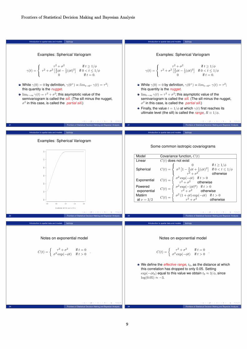
Examples: Spherical Variogram
γ(t) =
τ2 + σ2 if t ≥ 1/φ
τ2 + σ2[
32φt− 1
2(φt)3]
if 0 < t ≤ 1/φ0 if t = 0.
While γ(0) = 0 by definition, γ(0+) ≡ limt→0+ γ(t) = τ2;this quantity is the nugget.limt→∞ γ(t) = τ2 + σ2; this asymptotic value of thesemivariogram is called the sill. (The sill minus the nugget,σ2 in this case, is called the partial sill.)Finally, the value t = 1/φ at which γ(t) first reaches itsultimate level (the sill) is called the range, R ≡ 1/φ.
21 Frontiers of Statistical Decision Making and Bayesian Analysis
Introduction to spatial data and models Isotropy
Examples: Spherical Variogram
γ(t) =
τ2 + σ2 if t ≥ 1/φ
τ2 + σ2[
32φt− 1
2(φt)3]
if 0 < t ≤ 1/φ0 if t = 0.
While γ(0) = 0 by definition, γ(0+) ≡ limt→0+ γ(t) = τ2;this quantity is the nugget.
limt→∞ γ(t) = τ2 + σ2; this asymptotic value of thesemivariogram is called the sill. (The sill minus the nugget,σ2 in this case, is called the partial sill.)Finally, the value t = 1/φ at which γ(t) first reaches itsultimate level (the sill) is called the range, R ≡ 1/φ.
21 Frontiers of Statistical Decision Making and Bayesian Analysis
Frontiers of Statistical Decision Making and Bayesian Analysis
9
Frontiers of Statistical Decision Making and Bayesian Analysis
9
Introduction to spatial data and models Isotropy
Examples: Spherical Variogram
γ(t) =
τ2 + σ2 if t ≥ 1/φ
τ2 + σ2[
32φt− 1
2(φt)3]
if 0 < t ≤ 1/φ0 if t = 0.
While γ(0) = 0 by definition, γ(0+) ≡ limt→0+ γ(t) = τ2;this quantity is the nugget.limt→∞ γ(t) = τ2 + σ2; this asymptotic value of thesemivariogram is called the sill. (The sill minus the nugget,σ2 in this case, is called the partial sill.)
Finally, the value t = 1/φ at which γ(t) first reaches itsultimate level (the sill) is called the range, R ≡ 1/φ.
21 Frontiers of Statistical Decision Making and Bayesian Analysis
Introduction to spatial data and models Isotropy
Examples: Spherical Variogram
γ(t) =
τ2 + σ2 if t ≥ 1/φ
τ2 + σ2[
32φt− 1
2(φt)3]
if 0 < t ≤ 1/φ0 if t = 0.
While γ(0) = 0 by definition, γ(0+) ≡ limt→0+ γ(t) = τ2;this quantity is the nugget.limt→∞ γ(t) = τ2 + σ2; this asymptotic value of thesemivariogram is called the sill. (The sill minus the nugget,σ2 in this case, is called the partial sill.)Finally, the value t = 1/φ at which γ(t) first reaches itsultimate level (the sill) is called the range, R ≡ 1/φ.
21 Frontiers of Statistical Decision Making and Bayesian Analysis
Introduction to spatial data and models Isotropy
Examples: Spherical Variogram
0.0 0.5 1.0 1.5 2.0
0.0
0.2
0.4
0.6
0.8
1.0
1.2
b) spherical; a0 = 0.2 , a1 = 1 , R = 1
22 Frontiers of Statistical Decision Making and Bayesian Analysis
Introduction to spatial data and models Isotropy
Some common isotropic covariograms
Model Covariance function, C(t)Linear C(t) does not exist
Spherical C(t) =
0 if t ≥ 1/φ
σ2[1− 3
2φt+ 12(φt)3
]if 0 < t ≤ 1/φ
τ2 + σ2 otherwise
Exponential C(t) =σ2 exp(−φt) if t > 0τ2 + σ2 otherwise
Poweredexponential
C(t) =σ2 exp(−|φt|p) if t > 0
τ2 + σ2 otherwiseMatérnat ν = 3/2
C(t) =σ2 (1 + φt) exp(−φt) if t > 0
τ2 + σ2 otherwise
23 Frontiers of Statistical Decision Making and Bayesian Analysis
Introduction to spatial data and models Isotropy
Notes on exponential model
C(t) =
τ2 + σ2 if t = 0σ2 exp(−φt) if t > 0
.
We define the effective range, t0, as the distance at whichthis correlation has dropped to only 0.05. Settingexp(−φt0) equal to this value we obtain t0 ≈ 3/φ, sincelog(0.05) ≈ −3.Finally, the form of C(t) shows why the nugget τ2 is oftenviewed as a “nonspatial effect variance,” and the partial sill(σ2) is viewed as a “spatial effect variance.”
24 Frontiers of Statistical Decision Making and Bayesian Analysis
Introduction to spatial data and models Isotropy
Notes on exponential model
C(t) =
τ2 + σ2 if t = 0σ2 exp(−φt) if t > 0
.
We define the effective range, t0, as the distance at whichthis correlation has dropped to only 0.05. Settingexp(−φt0) equal to this value we obtain t0 ≈ 3/φ, sincelog(0.05) ≈ −3.
Finally, the form of C(t) shows why the nugget τ2 is oftenviewed as a “nonspatial effect variance,” and the partial sill(σ2) is viewed as a “spatial effect variance.”
24 Frontiers of Statistical Decision Making and Bayesian Analysis

Frontiers of Statistical Decision Making and Bayesian Analysis
10
Frontiers of Statistical Decision Making and Bayesian Analysis
10
Introduction to spatial data and models Isotropy
Notes on exponential model
C(t) =
τ2 + σ2 if t = 0σ2 exp(−φt) if t > 0
.
We define the effective range, t0, as the distance at whichthis correlation has dropped to only 0.05. Settingexp(−φt0) equal to this value we obtain t0 ≈ 3/φ, sincelog(0.05) ≈ −3.Finally, the form of C(t) shows why the nugget τ2 is oftenviewed as a “nonspatial effect variance,” and the partial sill(σ2) is viewed as a “spatial effect variance.”
24 Frontiers of Statistical Decision Making and Bayesian Analysis
Introduction to spatial data and models Isotropy
The Matèrn Correlation Function
Much of statistical modelling is carried out throughcorrelation functions rather than variograms
The Matèrn is a very versatile family:
C(t) =
σ2
2ν−1Γ(ν)(2√νtφ)νKν(2
√(ν)tφ) if t > 0
τ2 + σ2 if t = 0
Kν is the modified Bessel function of order ν(computationally tractable)ν is a smoothness parameter (a fractal) controlling processsmoothness
25 Frontiers of Statistical Decision Making and Bayesian Analysis
Introduction to spatial data and models Isotropy
The Matèrn Correlation Function
Much of statistical modelling is carried out throughcorrelation functions rather than variogramsThe Matèrn is a very versatile family:
C(t) =
σ2
2ν−1Γ(ν)(2√νtφ)νKν(2
√(ν)tφ) if t > 0
τ2 + σ2 if t = 0
Kν is the modified Bessel function of order ν(computationally tractable)
ν is a smoothness parameter (a fractal) controlling processsmoothness
25 Frontiers of Statistical Decision Making and Bayesian Analysis
Introduction to spatial data and models Isotropy
The Matèrn Correlation Function
Much of statistical modelling is carried out throughcorrelation functions rather than variogramsThe Matèrn is a very versatile family:
C(t) =
σ2
2ν−1Γ(ν)(2√νtφ)νKν(2
√(ν)tφ) if t > 0
τ2 + σ2 if t = 0
Kν is the modified Bessel function of order ν(computationally tractable)ν is a smoothness parameter (a fractal) controlling processsmoothness
25 Frontiers of Statistical Decision Making and Bayesian Analysis
Introduction to spatial data and models Variogram model fitting
How do we select a variogram? Can the data reallydistinguish between variograms?
Empirical Variogram:
γ(t) =1
2|N(t)|∑
si,sj∈N(t)
(Y (si)− Y (sj))2
where N(t) is the number of points such that ‖si − sj‖ = tand |N(t)| is the number of points in N(t).Grid up the t space into intervals I1 = (0, t1), I2 = (t1, t2),and so forth, up to IK = (tK−1, tK). Representing t valuesin each interval by its midpoint, we define:
N(tk) = (si,sj) : ‖si − sj‖ ∈ Ik, k = 1, . . . ,K.
26 Frontiers of Statistical Decision Making and Bayesian Analysis
Introduction to spatial data and models Variogram model fitting
How do we select a variogram? Can the data reallydistinguish between variograms?Empirical Variogram:
γ(t) =1
2|N(t)|∑
si,sj∈N(t)
(Y (si)− Y (sj))2
where N(t) is the number of points such that ‖si − sj‖ = tand |N(t)| is the number of points in N(t).
Grid up the t space into intervals I1 = (0, t1), I2 = (t1, t2),and so forth, up to IK = (tK−1, tK). Representing t valuesin each interval by its midpoint, we define:
N(tk) = (si,sj) : ‖si − sj‖ ∈ Ik, k = 1, . . . ,K.
26 Frontiers of Statistical Decision Making and Bayesian Analysis

Frontiers of Statistical Decision Making and Bayesian Analysis
11
Frontiers of Statistical Decision Making and Bayesian Analysis
11
Introduction to spatial data and models Variogram model fitting
How do we select a variogram? Can the data reallydistinguish between variograms?Empirical Variogram:
γ(t) =1
2|N(t)|∑
si,sj∈N(t)
(Y (si)− Y (sj))2
where N(t) is the number of points such that ‖si − sj‖ = tand |N(t)| is the number of points in N(t).Grid up the t space into intervals I1 = (0, t1), I2 = (t1, t2),and so forth, up to IK = (tK−1, tK). Representing t valuesin each interval by its midpoint, we define:
N(tk) = (si,sj) : ‖si − sj‖ ∈ Ik, k = 1, . . . ,K.
26 Frontiers of Statistical Decision Making and Bayesian Analysis
Introduction to spatial data and models Variogram model fitting
Empirical variogram: scallops data
distance
Gam
ma(
d)
0.0 0.5 1.0 1.5 2.0
01
23
45
6
27 Frontiers of Statistical Decision Making and Bayesian Analysis
Introduction to spatial data and models Variogram model fitting
Empirical variogram: scallops data
distance
gam
ma(
d)
0.0 0.5 1.0 1.5 2.0 2.5 3.0
02
46
8
Parametric Semivariograms
ExponentialGaussianCauchySphericalBessel-J0
distance
gam
ma(
d)
0.0 0.5 1.0 1.5 2.0 2.5 3.0
02
46
8
Bessel Mixtures - Random Weights
TwoThreeFourFive
distance
gam
ma(
d)
0.0 0.5 1.0 1.5 2.0 2.5 3.0
02
46
8
Bessel Mixtures - Random Phi’s
TwoThreeFourFive
28 Frontiers of Statistical Decision Making and Bayesian Analysis

Frontiers of Statistical Decision Making and Bayesian Analysis
12
Frontiers of Statistical Decision Making and Bayesian Analysis
12
Principles of Bayesian Inference
Sudipto Banerjee1 and Andrew O. Finley2
1 Biostatistics, School of Public Health, University of Minnesota, Minneapolis, Minnesota, U.S.A.
2 Department of Forestry & Department of Geography, Michigan State University, Lansing Michigan, U.S.A.
March 3, 2010
1
Bayesian principles
Classical statistics: model parameters are fixed andunknown.
A Bayesian thinks of parameters as random, and thushaving distributions (just like the data). We can thus thinkabout unknowns for which no reliable frequentistexperiment exists, e.g. θ = proportion of US men withuntreated prostate cancer.
A Bayesian writes down a prior guess for parameter(s) θ,say p(θ). He then combines this with the informationprovided by the observed data y to obtain the posteriordistribution of θ, which we denote by p(θ |y).
All statistical inferences (point and interval estimates,hypothesis tests) then follow from posterior summaries. Forexample, the posterior means/medians/modes offer pointestimates of θ, while the quantiles yield credible intervals.
2 Frontiers of Statistical Decision Making and Bayesian Analysis
Bayesian principles
The key to Bayesian inference is “learning” or “updating” ofprior beliefs. Thus, posterior information ≥ priorinformation.
Is the classical approach wrong? That may be acontroversial statement, but it certainly is fair to say thatthe classical approach is limited in scope.
The Bayesian approach expands the class of models andeasily handles:
repeated measuresunbalanced or missing datanonhomogenous variancesmultivariate data
– and many other settings that are precluded (or muchmore complicated) in classical settings.
3 Frontiers of Statistical Decision Making and Bayesian Analysis
Basics of Bayesian inference
We start with a model (likelihood) f(y |θ) for the observeddata y = (y1, . . . , yn)′ given unknown parameters θ(perhaps a collection of several parameters).
Add a prior distribution p(θ |λ), where λ is a vector ofhyper-parameters.
The posterior distribution of θ is given by:
p(θ |y,λ) =p(θ |λ)× f(y |θ)
p(y |λ)=
p(θ |λ)× f(y |θ)∫f(y |θ)p(θ |λ)dθ
.
We refer to this formula as Bayes Theorem.
4 Frontiers of Statistical Decision Making and Bayesian Analysis
Basics of Bayesian inference
Calculations (numerical and algebraic) are usually requiredonly up to a proportionaly constant. We, therefore, writethe posterior as:
p(θ |y,λ) ∝ p(θ |λ)× f(y |θ).
If λ are known/fixed, then the above represents the desiredposterior. If, however, λ are unknown, we assign a prior,p(λ), and seek:
p(θ,λ |y) ∝ p(λ)p(θ |λ)f(y |θ).
The proportionality constant does not depend upon θ or λ:1
p(y)=
1∫p(λ)p(θ |λ)f(y |θ)dλdθ
The above represents a joint posterior from a hierarchicalmodel. The marginal posterior distribution for θ is:
p(θ |y) =∫p(λ)p(θ |λ)f(y |θ)dλ.
5 Frontiers of Statistical Decision Making and Bayesian Analysis
Bayesian inference: point estimation
Point estimation is easy: simply choose an appropriatedistribution summary: posterior mean, median or mode.
Mode sometimes easy to compute (no integration, simplyoptimization), but often misrepresents the “middle” of thedistribution – especially for one-tailed distributions.
Mean: easy to compute. It has the “opposite effect” of themode – chases tails.
Median: probably the best compromise in being robust totail behaviour although it may be awkward to compute as itneeds to solve: ∫ θmedian
−∞p(θ |y)dθ =
12.
6 Frontiers of Statistical Decision Making and Bayesian Analysis

Frontiers of Statistical Decision Making and Bayesian Analysis
13
Frontiers of Statistical Decision Making and Bayesian Analysis
13
Bayesian inference: interval estimation
The most popular method of inference in practicalBayesian modelling is interval estimation using crediblesets. A 100(1− α)% credible set C for θ is a set thatsatisfies:
P (θ ∈ C |y) =∫Cp(θ |y)dθ ≥ 1− α.
The most popular credible set is the simple equal-tailinterval estimate (qL, qU ) such that:∫ qL
−∞p(θ |y)dθ =
α
2=∫ ∞qU
p(θ |y)dθ
Then clearly P (θ ∈ (qL, qU ) |y) = 1− α.This interval is relatively easy to compute and has a directinterpretation: The probability that θ lies between (qL, qU )is 1− α. The frequentist interpretation is extremelyconvoluted.
7 Frontiers of Statistical Decision Making and Bayesian Analysis
A simple example: Normal data and normal priors
Example: Consider a single data point y from a Normaldistribution: y ∼ N(θ, σ2); assume σ is known.
f(y|θ) = N(y | θ, σ2) =1
σ√
2πexp(− 1
2σ2(y − θ)2)
θ ∼ N(µ, τ2), i.e. p(θ) = N(θ |µ, τ2); µ, τ2 are known.Posterior distribution of θ
p(θ|y) ∝ N(θ |µ, τ2)×N(y | θ, σ2)
= N
(θ |
1τ2
1σ2 + 1
τ2
µ+1σ2
1σ2 + 1
τ2
y,1
1σ2 + 1
τ2
)
= N
(θ | σ2
σ2 + τ2µ+
τ2
σ2 + τ2y,
σ2τ2
σ2 + τ2
).
8 Frontiers of Statistical Decision Making and Bayesian Analysis
A simple example: Normal data and normal priors
Interpret: Posterior mean is a weighted mean of priormean and data point.The direct estimate is shrunk towards the prior.What if you had n observations instead of one in the earlierset up? Say y = (y1, . . . , yn)′, where yi
iid∼ N(0, σ2).
y is a sufficient statistic for µ; y ∼ N(µ, σ
2
n
)Posterior distribution of θ
p(θ |y) ∝ N(θ |µ, τ2)×N(y | θ, σ
2
n
)= N
(θ |
1τ2
nσ2 + 1
τ2
µ+nσ2
nσ2 + 1
τ2
y,1
nσ2 + 1
τ2
)
= N
(θ | σ2
σ2 + nτ2µ+
nτ2
σ2 + nτ2y,
σ2τ2
σ2 + nτ2
)
9 Frontiers of Statistical Decision Making and Bayesian Analysis
Another simple example: The Beta-Binomial model
Example: Let Y be the number of successes in nindependent trials.
P (Y = y|θ) = f(y|θ) =(n
y
)θy(1− θ)n−y
Prior: p(θ) = Beta(θ|a, b):
p(θ) ∝ θa−1(1− θ)b−1.
Prior mean: µ = a/(a+ b); Variance ab/((a+ b)2(a+ b+ 1))Posterior distribution of θ
p(θ|y) = Beta(θ|a+ y, b+ n− y)
10 Frontiers of Statistical Decision Making and Bayesian Analysis
Sampling-based inference
We will compute the posterior distribution p(θ |y) bydrawing samples from it. This replaces numericalintegration (quadrature) by “Monte Carlo integration”.
One important advantage: we only need to know p(θ |y)up to the proportionality constant.
Suppose θ = (θ1,θ2) and we know how to sample fromthe marginal posterior distribution p(θ2|y) and theconditional distribution P (θ1 |θ2,y).
How do we draw samples from the joint distribution:p(θ1,θ2 |y)?
11 Frontiers of Statistical Decision Making and Bayesian Analysis
Sampling-based inference
We do this in two stages using composition sampling:
First draw θ(j)2 ∼ p(θ2 |y), j = 1, . . .M .
Next draw θ(j)1 ∼ p
(θ1 |θ(j)
2 ,y)
.
This sampling scheme produces exact samples,θ(j)
1 ,θ(j)2 Mj=1 from the posterior distribution p(θ1,θ2 |y).
Gelfand and Smith (JASA, 1990) demonstrated automaticmarginalization: θ(j)
1 Mj=1 are samples from p(θ1 |y) and
(of course!) θ(j)2 Mj=1 are samples from p(θ2 |y).
In effect, composition sampling has performed thefollowing “integration”:
p(θ1 |y) =∫p(θ1 |θ2,y)p(θ2 |y)dθ.
12 Frontiers of Statistical Decision Making and Bayesian Analysis

Frontiers of Statistical Decision Making and Bayesian Analysis
14
Frontiers of Statistical Decision Making and Bayesian Analysis
14
Bayesian predictions
Suppose we want to predict new observations, say y,based upon the observed data y. We will specify a jointprobability model p(y,y | ,θ), which defines the conditionalpredictive distribution:
p(y |y,θ) =p(y,y | ,θ)p(y |θ)
.
Bayesian predictions follow from the posterior predictivedistribution that averages out the θ from the conditionalpredictive distribution with respect to the posterior:
p(y |y) =∫p(y |y,θ)p(θ |y)dθ.
This can be evaluated using composition sampling:First obtain: θ(j) ∼ p(θ |y), j = 1, . . .MFor j = 1, . . . ,M sample y(j) ∼ p(y |y,θ(j))
The y(j)Mj=1 are samples from the posterior predictivedistribution p(y |y).
13 Frontiers of Statistical Decision Making and Bayesian Analysis
Some remarks on sampling-based inference
Direct Monte Carlo: Some algorithms (e.g. composition sampling) can generate independent samplesexactly from the posterior distribution. In these situations there are NO convergence problems or issues.Sampling is called exact.
Markov Chain Monte Carlo (MCMC): In general, exact sampling may not be possible/feasible. MCMC is afar more versatile set of algorithms that can be invoked to fit more general models. Note: anywhere wheredirect Monte Carlo applies, MCMC will provide excellent results too.
Convergence issues: There is no free lunch! The power of MCMC comes at a cost. The initial samples donot necessarily come from the desired posterior distribution. Rather, they need to converge to the trueposterior distribution. Therefore, one needs to assess convergence, discard output before the convergenceand retain only post-convergence samples. The time of convergence is called burn-in.
Diagnosing convergence: Usually a few parallel chains are run from rather different starting points. Thesample values are plotted (called trace-plots) for each of the chains. The time for the chains to “mix”together is taken as the time for convergence.
Good news! All this is automated in WinBUGS. So, as users, we need to only configure how to specify goodBayesian models and implement them in WinBUGS.
14 Frontiers of Statistical Decision Making and Bayesian Analysis
Frontiers of Statistical Decision Making and Bayesian Analysis
15
Frontiers of Statistical Decision Making and Bayesian Analysis
15
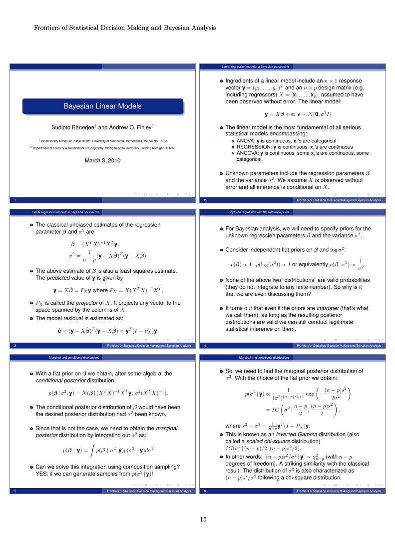
Bayesian Linear Models
Sudipto Banerjee1 and Andrew O. Finley2
1 Biostatistics, School of Public Health, University of Minnesota, Minneapolis, Minnesota, U.S.A.
2 Department of Forestry & Department of Geography, Michigan State University, Lansing Michigan, U.S.A.
March 3, 2010
1
Linear regression models: a Bayesian perspective
Ingredients of a linear model include an n× 1 responsevector y = (y1, . . . , yn)T and an n× p design matrix (e.g.including regressors) X = [x1, . . . ,xp], assumed to havebeen observed without error. The linear model:
y = Xβ + ε; ε ∼ N(0, σ2I)
The linear model is the most fundamental of all seriousstatistical models encompassing:
ANOVA: y is continuous, xi’s are categoricalREGRESSION: y is continuous, xi’s are continuousANCOVA: y is continuous, some xi’s are continuous, somecategorical.
Unknown parameters include the regression parameters βand the variance σ2. We assume X is observed withouterror and all inference is conditional on X.
2 Frontiers of Statistical Decision Making and Bayesian Analysis
Linear regression models: a Bayesian perspective
The classical unbiased estimates of the regressionparameter β and σ2 are
β = (XTX)−1XT y;
σ2 =1
n− p(y−Xβ)T (y−Xβ).
The above estimate of β is also a least-squares estimate.The predicted value of y is given by
y = Xβ = PXy where PX = X(XTX)−1XT .
PX is called the projector of X. It projects any vector to thespace spanned by the columns of X.The model residual is estimated as:
e = (y−Xβ)T (y−Xβ) = yT (I − PX)y.
3 Frontiers of Statistical Decision Making and Bayesian Analysis
Bayesian regression with flat reference priors
For Bayesian analysis, we will need to specify priors for theunknown regression parameters β and the variance σ2.
Consider independent flat priors on β and log σ2:
p(β) ∝ 1; p(log(σ2)) ∝ 1 or equivalently p(β, σ2) ∝ 1σ2.
None of the above two “distributions” are valid probabilities(they do not integrate to any finite number). So why is itthat we are even discussing them?
It turns out that even if the priors are improper (that’s whatwe call them), as long as the resulting posteriordistributions are valid we can still conduct legitimatestatistical inference on them.
4 Frontiers of Statistical Decision Making and Bayesian Analysis
Marginal and conditional distributions
With a flat prior on β we obtain, after some algebra, theconditional posterior distribution:
p(β |σ2,y) = N(β | (XTX)−1XT y, σ2(XTX)−1).
The conditional posterior distribution of β would have beenthe desired posterior distribution had σ2 been known.
Since that is not the case, we need to obtain the marginalposterior distribution by integrating out σ2 as:
p(β | y) =∫p(β | σ2,y)p(σ2 | y)dσ2
Can we solve this integration using composition sampling?YES: if we can generate samples from p(σ2 |y)!
5 Frontiers of Statistical Decision Making and Bayesian Analysis
Marginal and conditional distributions
So, we need to find the marginal posterior distribution ofσ2. With the choice of the flat prior we obtain:
p(σ2 |y) ∝ 1(σ2)(n−p)/2+1
exp(−(n− p)s2
2σ2
)= IG
(σ2 | n− p
2,(n− p)s2
2
),
where s2 = σ2 = 1n−pyT (I − PX)y.
This is known as an inverted Gamma distribution (alsocalled a scaled chi-square distribution)IG(σ2 | (n− p)/2, (n− p)s2/2).In other words: [(n− p)s2/σ2 |y] ∼ χ2
n−p (with n− pdegrees of freedom). A striking similarity with the classicalresult: The distribution of σ2 is also characterized as(n− p)s2/σ2 following a chi-square distribution.
6 Frontiers of Statistical Decision Making and Bayesian Analysis

Frontiers of Statistical Decision Making and Bayesian Analysis
16
Frontiers of Statistical Decision Making and Bayesian Analysis
16
Composition sampling for linear regression
Now we are ready to carry out composittion sampling fromp(β, σ2 |y) as follows:
Draw M samples from p(σ2 |y):
σ2(j) ∼ IG(n− p
2,
(n− p)s22
(n− p)), j = 1, . . .M
For j = 1, . . . ,M , draw from p(β |σ2(j),y):
β(j) ∼ N(
(XTX)−1XT y, σ2(j)(XTX)−1)
The resulting samples β(j), σ2(j)Mj=1 represent Msamples from p(β, σ2 |y).β(j)Mj=1 are samples from the marginal posteriordistribution p(β |y). This is a multivariate t density:
p(β | y) =Γ(n/2)
(π(n− p))p/2Γ((n− p)/2)|s2(XTX)−1|
"1 +
(β − β)T (XTX)(β − β)
(n− p)s2
#−n/2
.
7 Frontiers of Statistical Decision Making and Bayesian Analysis
Composition sampling for linear regression
The marginal distribution of each individual regressionparameter βj is a non-central univariate tn−p distribution.In fact,
βj − βj
s√
(XTX)−1jj
∼ tn−p.
The 95% credible intervals for each βj are constructedfrom the quantiles of the t-distribution. The credibleintervals exactly coicide with the 95% classical confidenceintervals, but the intepretation is direct: the probability of βj
falling in that interval, given the observed data, is 0.95.
Note: an intercept only linear model reduces to the simpleunivariate N(y |µ, σ2/n) likelihood, for which the marginalposterior of µ is:
µ− ys/√n∼ tn−1.
8 Frontiers of Statistical Decision Making and Bayesian Analysis
Bayesian predictions from the linear model
Suppose we have observed the new predictors X, and wewish to predict the outcome y. We specify p(y,y |θ) to be anormal distribution:(
yy
)∼ N
([X
X
]β, σ2I
)Note p(y |y,β, σ2) = p(y |β, σ2) = N(y | Xβ, σ2I).
The posterior predictive distribution:
p(y |y) =∫p(y |y,β, σ2)p(β, σ2 |y)dβdσ2
=∫p(y |β, σ2)p(β, σ2 |y)dβdσ2.
By now we are comfortable evaluating such integrals:First obtain: (β(j), σ2(j)) ∼ p(β, σ2 |y), j = 1, . . . ,MNext draw: y(j) ∼ N(Xβ(j), σ2(j)I).
9 Frontiers of Statistical Decision Making and Bayesian Analysis
The Gibbs sampler
Suppose that θ = (θ1,θ2) and we seek the posteriordistribution p(θ1,θ2 |y).
For many interesting hierarchical models, we have accessto full conditional distributions p(θ1 |θ2,y) and p(θ1 |θ2,y).
The Gibbs sampler proposes the following samplingscheme. Set starting values θ(0) = (θ(0)
1 ,θ(0)2 ) For
j = 1, . . . ,MDraw θ
(j)1 ∼ p(θ1 |θ(j−1)
2 ,y)Draw θ
(j)2 ∼ p(θ2 |θ(j)
1 ,y)
This constructs a Markov Chain and, after an initial“burn-in” period when the chains are trying to find theirway, the above algorithm guarantees thatθ(j)
1 ,θ(j)2 Mj=M0+1 will be samples from p(θ1,θ2 |y), where
M0 is the burn-in period..
10 Frontiers of Statistical Decision Making and Bayesian Analysis
The Gibbs sampler
More generally, if θ = (θ1, . . . ,θp) are the parameters inour model, we provide a set of initial valuesθ(0) = (θ(0)
1 , . . . ,θ(0)p ) and then performs the j-th iteration,
say for j = 1, . . . ,M , by updating successively from the fullconditional distributions:
θ(j)1 ∼ p(θ(j)
1 |θ(j−1)2 , . . . ,θ
(j−1)p ,y)
θ(j)2 ∼ p(θ2 |θ(j)
1 ,θ(j)3 , . . . ,θ
(j−1)p ,y)
. . .(the generic kth element)θ
(j)k ∼ p(θk|θ(j)
1 , . . . ,θ(j)k−1,θ
(j)k+1, . . . ,θ
(j−1)p ,y)
· · ·θ
(j)p ∼ p(θp |θ(j)
1 , . . . ,θ(j)p−1,y)
11 Frontiers of Statistical Decision Making and Bayesian Analysis
The Gibbs sampler
Example: Consider the linear model. Suppose we setp(σ2) = IG(σ2 | a, b) and p(β) ∝ 1.
The full conditional distributions are:
p(β |y, σ2) = N(β | (XTX)−1XT y, σ2(XTX)−1)
p(σ2 |y,β) = IG
(σ2 | a+ n/2, b+
12
(y−Xβ)T (y−Xβ)).
Thus, the Gibbs sampler will initialize (β(0), σ2(0)) anddraw, for j = 1, . . . ,M :
Draw β(j) ∼ N((XTX)−1XT y, σ2(j−1)(XTX)−1)Draw σ2(j) ∼ IG
(a+ n/2, b+ 1
2 (y−Xβ(j))T (y−Xβ(j)))
12 Frontiers of Statistical Decision Making and Bayesian Analysis

Frontiers of Statistical Decision Making and Bayesian Analysis
17
Frontiers of Statistical Decision Making and Bayesian Analysis
17
The Gibbs sampler
In principle, the Gibbs sampler will work for extremelycomplex hierarchical models. The only issue is samplingfrom the full conditionals. They may not be amenable toeasy sampling – when these are not in closed form. Amore general and extremely powerful - and often easier tocode - algorithm is the Metropolis-Hastings (MH) algorithm.
This algorithm also constructs a Markov Chain, but doesnot necessarily care about full conditionals.
13 Frontiers of Statistical Decision Making and Bayesian Analysis
The Metropolis-Hastings algorithm
The Metropolis-Hastings algorithm: Start with a initial value for θ = θ(0).Select a candidate or proposal distribution from which to propose avalue of θ at the j-th iteration: θ(j) ∼ q(θ(j−1), ν). For example,q(θ(j−1), ν) = N(θ(j−1), ν) with ν fixed.
Compute
r =p(θ∗ | y)q(θ(j−1) |θ∗, ν)p(θ(j−1) | y)q(θ∗ |θ(j−1)ν)
If r ≥ 1 then set θ(j) = θ∗. If r ≤ 1 then draw U ∼ (0, 1). If U ≤ r thenθ(j) = θ∗. Otherwise, θ(j) = θ(j−1).
Repeat for j = 1, . . .M . This yields θ(1), . . . ,θ(M), which, after aburn-in period, will be samples from the true posterior distribution. It isimportant to monitor the acceptance ratio r of the sampler through theiterations. Rough recommendations: for vector updates r ≈ 20%., forscalar updates r ≈ 40%. This can be controlled by “tuning” ν.
Popular approach: Embed Metropolis steps within Gibbs to draw fromfull conditionals that are not accessible to directly generate from.
14 Frontiers of Statistical Decision Making and Bayesian Analysis
The Metropolis-Hastings algorithm
Example: For the linear model, our parameters are (β, σ2). We write θ = (β, log(σ2)) and, at the j-thiteration, propose θ∗ ∼ N(θ(j−1),Σ). The log transformation on σ2 ensures that all components of θhave support on the entire real line and can have meaningful proposed values from the multivariate normal.But we need to transform our prior to p(β, log(σ2)).
Let z = log(σ2) and assume p(β, z) = p(β)p(z). Let us derive p(z). REMEMBER: we need to adjustfor the jacobian. Then p(z) = p(σ2)|dσ2/dz| = p(ez)ez . The jacobian here is ez = σ2.
Let p(β) = 1 and an p(σ2) = IG(σ2 | a, b). Then log-posterior is:
−(a + n/2 + 1)z + z − 1
ezb +
1
2(Y −Xβ)
T(Y −Xβ).
A symmetric proposal distribution, say q(θ∗|θ(j−1),Σ) = N(θ(j−1),Σ), cancels out in r. In practiceit is better to compute log(r): log(r) = log(p(θ∗ | y)− log(p(θ(j−1) | y)). For the proposal,N(θ(j−1),Σ), Σ is a d× d variance-covariance matrix, and d = dim(θ) = p + 1.
If log r ≥ 0 then set θ(j) = θ∗. If log r ≤ 0 then draw U ∼ (0, 1). If U ≤ r (or logU ≤ log r) thenθ(j) = θ∗. Otherwise, θ(j) = θ(j−1).
Repeat the above procedure for j = 1, . . .M to obtain samples θ(1), . . . , θ(M).
15 Frontiers of Statistical Decision Making and Bayesian Analysis

Frontiers of Statistical Decision Making and Bayesian Analysis
18
Frontiers of Statistical Decision Making and Bayesian Analysis
18
Hierarchical Modelling for Univariate SpatialData
Sudipto Banerjee1 and Andrew O. Finley2
1 Biostatistics, School of Public Health, University of Minnesota, Minneapolis, Minnesota, U.S.A.
2 Department of Forestry & Department of Geography, Michigan State University, Lansing Michigan, U.S.A.
March 3, 2010
1
Univariate spatial models
Spatial Domain
0 2 4 6 8 10
02
46
810
x
y
2 Frontiers of Statistical Decision Making and Bayesian Analysis
Univariate spatial models
Algorithmic Modelling
Spatial surface observed at finite set of locationsS = s1, s2, ..., snTessellate the spatial domain (usually with data locationsas vertices)Fit an interpolating polynomial:
f(s) =∑
i
wi(S ; s)f(si)
“Interpolate” by reading off f(s0).Issues:
Sensitivity to tessellationsChoices of multivariate interpolatorsNumerical error analysis
3 Frontiers of Statistical Decision Making and Bayesian Analysis
Univariate spatial models
What is a spatial process?
x
x
x
x
Y(s1)
Y(s2)
Y(sn)
4 Frontiers of Statistical Decision Making and Bayesian Analysis
Univariate spatial models Simple linear model
Simple linear model
Y (s) = µ(s) + ε(s),
Response: Y (s) at location sMean: µ = xT (s)β
Error: ε(s) iid∼ N(0, τ2)
D
Y (s), x(s)
5 Frontiers of Statistical Decision Making and Bayesian Analysis
Univariate spatial models Simple linear model
Simple linear model
Y (s) = µ(s) + ε(s),
Assumptions regarding ε(s):
ε(s) iid∼ N(0, τ2)
ε(si) and ε(sj) are uncorrelated for all i 6= j
D
ε(si)ε(sj)
6 Frontiers of Statistical Decision Making and Bayesian Analysis

Frontiers of Statistical Decision Making and Bayesian Analysis
19
Frontiers of Statistical Decision Making and Bayesian Analysis
19
Univariate spatial models Simple linear model
Simple linear model
Y (s) = µ(s) + ε(s),
Assumptions regarding ε(s):
ε(s) iid∼ N(0, τ2)ε(si) and ε(sj) are uncorrelated for all i 6= j
D
ε(si)ε(sj)
6 Frontiers of Statistical Decision Making and Bayesian Analysis
Univariate spatial models Sources of variation
Spatial Gaussian processes (GP ):Say w(s) ∼ GP (0, σ2ρ(·)) and
Cov(w(s1), w(s2)) = σ2ρ (φ; ‖s1 − s2‖)
Let w = [w(si)]ni=1, then
w ∼ N(0, σ2R(φ)), where R(φ) = [ρ(φ; ‖si − sj‖)]ni,j=1
D
w(si)w(sj)
7 Frontiers of Statistical Decision Making and Bayesian Analysis
Univariate spatial models Sources of variation
Realization of a Gaussian process:
Changing φ and holding σ2 = 1:
w ∼ N(0, σ2R(φ)), whereR(φ) = [ρ(φ; ‖si − sj‖)]ni,j=1
Correlation model for R(φ):e.g., exponential decay
ρ(φ; t) = exp(−φt) if t > 0.
Other valid models e.g., Gaussian,Spherical, Matérn.Effective range,t0 = ln(0.05)/φ ≈ 3/φ
8 Frontiers of Statistical Decision Making and Bayesian Analysis

Frontiers of Statistical Decision Making and Bayesian Analysis
20
Frontiers of Statistical Decision Making and Bayesian Analysis
20
Univariate spatial models Sources of variation
w ∼ N(0, σ2wR(φ)) defines complex spatial dependence
structures.
E.g., anisotropic Matérn correlation function:ρ(si, sj ; φ) =
`1/Γ(ν)2ν−1
´ “2pνdij)
νκν(2pνdij
”, where
dij = (si − sj)′ Σ−1 (si − sj), Σ = G(ψ)Λ2G(ψ)′. Thus, φ = (ν, ψ,Λ).
Simulated Predicted
9 Frontiers of Statistical Decision Making and Bayesian Analysis
Univariate spatial models Univariate spatial regression
Simple linear model + random spatial effects
Y (s) = µ(s) + w(s) + ε(s),
Response: Y (s) at some site
Mean: µ = xT (s)β
Spatial random effects: w(s) ∼ GP (0, σ2ρ(φ; ‖s1 − s2‖))
Non-spatial variance: ε(s) iid∼ N(0, τ2)
10 Frontiers of Statistical Decision Making and Bayesian Analysis
Univariate spatial models Univariate spatial regression
Hierarchical modelling
First stage:
y|β,w, τ2 ∼n∏
i=1
N(Y (si) |xT (si)β + w(si), τ2)
Second stage:
w|σ2, φ ∼ N(0, σ2R(φ))
Third stage: Priors on Ω = (β, τ2, σ2, φ)Marginalized likelihood:
y|Ω ∼ N(Xβ, σ2R(φ) + τ2I)
Note: Spatial process parametrizes Σ:y = Xβ + ε, ε ∼ N (0,Σ) , Σ = σ2R(φ) + τ2I
11 Frontiers of Statistical Decision Making and Bayesian Analysis
Univariate spatial models Univariate spatial regression
Hierarchical modelling
First stage:
y|β,w, τ2 ∼n∏
i=1
N(Y (si) |xT (si)β + w(si), τ2)
Second stage:
w|σ2, φ ∼ N(0, σ2R(φ))
Third stage: Priors on Ω = (β, τ2, σ2, φ)
Marginalized likelihood:
y|Ω ∼ N(Xβ, σ2R(φ) + τ2I)
Note: Spatial process parametrizes Σ:y = Xβ + ε, ε ∼ N (0,Σ) , Σ = σ2R(φ) + τ2I
11 Frontiers of Statistical Decision Making and Bayesian Analysis
Univariate spatial models Univariate spatial regression
Hierarchical modelling
First stage:
y|β,w, τ2 ∼n∏
i=1
N(Y (si) |xT (si)β + w(si), τ2)
Second stage:
w|σ2, φ ∼ N(0, σ2R(φ))
Third stage: Priors on Ω = (β, τ2, σ2, φ)Marginalized likelihood:
y|Ω ∼ N(Xβ, σ2R(φ) + τ2I)
Note: Spatial process parametrizes Σ:y = Xβ + ε, ε ∼ N (0,Σ) , Σ = σ2R(φ) + τ2I
11 Frontiers of Statistical Decision Making and Bayesian Analysis

Frontiers of Statistical Decision Making and Bayesian Analysis
21
Frontiers of Statistical Decision Making and Bayesian Analysis
21
Univariate spatial models Univariate spatial regression
Hierarchical modelling
First stage:
y|β,w, τ2 ∼n∏
i=1
N(Y (si) |xT (si)β + w(si), τ2)
Second stage:
w|σ2, φ ∼ N(0, σ2R(φ))
Third stage: Priors on Ω = (β, τ2, σ2, φ)Marginalized likelihood:
y|Ω ∼ N(Xβ, σ2R(φ) + τ2I)
Note: Spatial process parametrizes Σ:y = Xβ + ε, ε ∼ N (0,Σ) , Σ = σ2R(φ) + τ2I
11 Frontiers of Statistical Decision Making and Bayesian Analysis
Univariate spatial models Univariate spatial regression
Bayesian Computations
Choice: Fit [y|Ω]× [Ω] or [y|β,w, τ2]× [w|σ2, φ]× [Ω].
Conditional model:conjugate full conditionals for σ2, τ2 and w – easier toprogram.
Marginalized model:
need Metropolis or Slice sampling for σ2, τ2 and φ. Harderto program.But, reduced parameter space⇒ faster convergenceσ2R(φ) + τ2I is more stable than σ2R(φ).
But what about R−1(φ) ?? EXPENSIVE!
12 Frontiers of Statistical Decision Making and Bayesian Analysis
Univariate spatial models Univariate spatial regression
Where are the w’s?
Interest often lies in the spatial surface w|y.
They are recovered from
[w|y, X] =∫
[w|Ω,y, X]× [Ω|y, X]dΩ
using posterior samples:Obtain Ω(1), . . . ,Ω(G) ∼ [Ω|y, X]For each Ω(g), draw w(g) ∼ [w|Ω(g),y, X]
NOTE: With Gaussian likelihoods [w|Ω,y, X] is alsoGaussian. With other likelihoods this may not be easy andoften the conditional updating scheme is preferred.
13 Frontiers of Statistical Decision Making and Bayesian Analysis

Frontiers of Statistical Decision Making and Bayesian Analysis
22
Frontiers of Statistical Decision Making and Bayesian Analysis
22
Univariate spatial models Univariate spatial regression
Where are the w’s?
Interest often lies in the spatial surface w|y.
They are recovered from
[w|y, X] =∫
[w|Ω,y, X]× [Ω|y, X]dΩ
using posterior samples:
Obtain Ω(1), . . . ,Ω(G) ∼ [Ω|y, X]For each Ω(g), draw w(g) ∼ [w|Ω(g),y, X]
NOTE: With Gaussian likelihoods [w|Ω,y, X] is alsoGaussian. With other likelihoods this may not be easy andoften the conditional updating scheme is preferred.
13 Frontiers of Statistical Decision Making and Bayesian Analysis
Univariate spatial models Univariate spatial regression
Where are the w’s?
Interest often lies in the spatial surface w|y.
They are recovered from
[w|y, X] =∫
[w|Ω,y, X]× [Ω|y, X]dΩ
using posterior samples:Obtain Ω(1), . . . ,Ω(G) ∼ [Ω|y, X]For each Ω(g), draw w(g) ∼ [w|Ω(g),y, X]
NOTE: With Gaussian likelihoods [w|Ω,y, X] is alsoGaussian. With other likelihoods this may not be easy andoften the conditional updating scheme is preferred.
13 Frontiers of Statistical Decision Making and Bayesian Analysis
Univariate spatial models Univariate spatial regression
Residual plot: [w(s)|y]
Easting Northi
ng
w mean of Ymean of Ymean of Ymean of Ymean of Ymean of Ymean of Ymean of Ymean of Ymean of Ymean of Ymean of Ymean of Ymean of Ymean of Ymean of Ymean of Ymean of Ymean of Ymean of Ymean of Ymean of Ymean of Ymean of Ymean of Y
14 Frontiers of Statistical Decision Making and Bayesian Analysis
Univariate spatial models Univariate spatial regression
Another look: [w(s)|y]
Easting
Nort
hing
w
15 Frontiers of Statistical Decision Making and Bayesian Analysis
Univariate spatial models Univariate spatial regression
Another look: [w(s)|y]
Easting
Nort
hing
w
16 Frontiers of Statistical Decision Making and Bayesian Analysis

Frontiers of Statistical Decision Making and Bayesian Analysis
23
Frontiers of Statistical Decision Making and Bayesian Analysis
23
Univariate spatial models Spatial Prediction
Often we need to predict Y (s) at a new set of locationss0, . . . , sm with associated predictor matrix X.
Sample from predictive distribution:
[y|y, X, X] =∫
[y,Ω|y, X, X]dΩ
=∫
[y|y,Ω, X, X]× [Ω|y, X]dΩ,
[y|y,Ω, X, X] is multivariate normal. Sampling scheme:Obtain Ω(1), . . . ,Ω(G) ∼ [Ω|y, X]For each Ω(g), draw y(g) ∼ [y|y,Ω(g), X, X].
17 Frontiers of Statistical Decision Making and Bayesian Analysis
Univariate spatial models Spatial Prediction
Prediction: Summary of [Y (s)|y]
Easting
Nort
hing
y
18 Frontiers of Statistical Decision Making and Bayesian Analysis
Univariate spatial models Illustration
Colorado data illustration
Modelling temperature: 507 locations in Colorado.Simple spatial regression model:
Y (s) = xT (s)β + w(s) + ε(s)
w(s) ∼ GP (0, σ2ρ(·;φ, ν)); ε(s) iid∼ N(0, τ2)
Parameters 50% (2.5%,97.5%)Intercept 2.827 (2.131,3.866)
[Elevation] -0.426 (-0.527,-0.333)Precipitation 0.037 (0.002,0.072)
σ2 0.134 (0.051, 1.245)φ 7.39E-3 (4.71E-3, 51.21E-3)
Range 278.2 (38.8, 476.3)τ2 0.051 (0.022, 0.092)
19 Frontiers of Statistical Decision Making and Bayesian Analysis
Univariate spatial models Illustration
Temperature residual map
−300 −200 −100 0 100 200 300
4100
4200
4300
4400
4500
Easting
Nor
thin
g
20 Frontiers of Statistical Decision Making and Bayesian Analysis
Univariate spatial models Illustration
Elevation map
−108 −106 −104 −102
3738
3940
41
Longitude
Latit
ude
21 Frontiers of Statistical Decision Making and Bayesian Analysis
Univariate spatial models Illustration
Residual map with elev. as covariate
−300 −200 −100 0 100 200 300
4100
4200
4300
4400
4500
Easting
Nor
thin
g
22 Frontiers of Statistical Decision Making and Bayesian Analysis

Frontiers of Statistical Decision Making and Bayesian Analysis
24
Frontiers of Statistical Decision Making and Bayesian Analysis
24
Hierarchical Modelling for non-GaussianSpatial Data
Sudipto Banerjee1 and Andrew O. Finley2
1 Biostatistics, School of Public Health, University of Minnesota, Minneapolis, Minnesota, U.S.A.
2 Department of Forestry & Department of Geography, Michigan State University, Lansing Michigan, U.S.A.
March 3, 2010
1
Spatial Generalized Linear Models
Often data sets preclude Gaussian modelling: Y (s) maynot even be continuous
Example: Y (s) is a binary or count variable
species presence or absence at location sspecies abundance from count at location scontinuous forest variable is high or low at location s
Replace Gaussian likelihood by exponential family member
Diggle Tawn and Moyeed (1998)
2 Frontiers of Statistical Decision Making and Bayesian Analysis
Spatial Generalized Linear Models
First stage: Y (si) are conditionally independent given βand w(si), so f(y(si)|β, w(si), γ) equals
h(y(si), γ) exp (γ[y(si)η(si)− ψ(η(si))])
where g(E(Y (si))) = η(si) = xT (si)β + w(si) (canonicallink function) and γ is a dispersion parameter.Second stage: Model w(s) as a Gaussian process:
w ∼ N(0, σ2R(φ))
Third stage: Priors and hyperpriors.No process for Y (s), only a valid joint distributionNot sensible to add a pure error term ε(s)
3 Frontiers of Statistical Decision Making and Bayesian Analysis
Spatial Generalized Linear Models Comments
We are modelling with spatial random effectsIntroducing these in the transformed mean encouragesmeans of spatial variables at proximate locations to beclose to each otherMarginal spatial dependence is induced between, say,Y (s) and Y (s′), but observed Y (s) and Y (s′) need not beclose to each otherSecond stage spatial modelling is attractive for spatialexplanation in themeanFirst stage spatial modelling more appropriate toencourage proximate observations to be close.
4 Frontiers of Statistical Decision Making and Bayesian Analysis
Illustration
Illustration from:
Finley, A.O., S. Banerjee, and R.E. McRoberts. (2008) ABayesian approach to quantifying uncertainty in multi-sourceforest area estimates. Environmental and Ecological Statistics,15:241–258.
5 Frontiers of Statistical Decision Making and Bayesian Analysis
Illustration
Binary spatial regression: forest/non-forest
We illustrate a non-Gaussian model for point-referenced spatialdata:
Objective is to make pixel-level prediction offorest/non-forest across the domain.
Data: Observations are from 500 georeferenced USDAForest Service Forest Inventory and Analysis (FIA)inventory plots within a 32 km radius circle in MN, USA.The response Y (s) is a binary variable, with
Y (s) =
1 if inventory plot is forested0 if inventory plot is not forested
Observed covariates include the coinsiding pixel values for3 dates of 30× 30 m resolution Landsat imagery.
6 Frontiers of Statistical Decision Making and Bayesian Analysis

Frontiers of Statistical Decision Making and Bayesian Analysis
25
Frontiers of Statistical Decision Making and Bayesian Analysis
25
Illustration
Binary spatial regression: forest/non-forest
We illustrate a non-Gaussian model for point-referenced spatialdata:
Objective is to make pixel-level prediction offorest/non-forest across the domain.Data: Observations are from 500 georeferenced USDAForest Service Forest Inventory and Analysis (FIA)inventory plots within a 32 km radius circle in MN, USA.The response Y (s) is a binary variable, with
Y (s) =
1 if inventory plot is forested0 if inventory plot is not forested
Observed covariates include the coinsiding pixel values for3 dates of 30× 30 m resolution Landsat imagery.
6 Frontiers of Statistical Decision Making and Bayesian Analysis
Illustration
Binary spatial regression: forest/non-forest
We fit a generalized linear model whereY (si) ∼ Bernoulli(p(si)), logit(p(si)) = xT (si)β + w(si).
Assume vague flat for β, a Uniform(3/32, 3/0.5) prior for φ,and an inverse-Gamma(2, ·) prior for σ2.
Parameters updated with Metropolis algorithm using targetlog density:
ln (p(Ω |Y )) ∝−“σa + 1 +
n
2
”ln`σ2´− σb
σ2− 1
2ln (|R(φ)|)− 1
2σ2wTR(φ)−1w
+
nXi=1
Y (si)“
xT (si)β + w(si)”−
nXi=1
ln“1 + exp(xT (si)β + w(si)
”+ ln(σ2) + ln(φ− φa) + ln(φb − φ).
7 Frontiers of Statistical Decision Making and Bayesian Analysis
Illustration
Posterior parameter estimates
Parameter estimates (posterior medians and upper and lower2.5 percentiles):
Parameters Estimates: 50% (2.5%, 97.5%)Intercept (θ0) 82.39 (49.56, 120.46)AprilTC1 (θ1) -0.27 (-0.45, -0.11)AprilTC2 (θ2) 0.17 (0.07, 0.29)AprilTC3 (θ3) -0.24 (-0.43, -0.08)JulyTC1 (θ4) -0.04 (-0.25, 0.17)JulyTC2 (θ5) 0.09 (-0.01, 0.19)JulyTC3 (θ6) 0.01 (-0.15, 0.16)OctTC1 (θ7) -0.43 (-0.68, -0.22)OctTC2 (θ8) -0.03 (-0.19, 0.14)OctTC3 (θ9) -0.26 (-0.46, -0.07)
σ2 1.358 (0.39, 2.42)φ 0.00182 (0.00065, 0.0032)
log(0.05)/φ (meters) 1644.19 (932.33, 4606.7)
Covariates and proximity to observed FIA plot will contribute toincrease precision of prediction.
8 Frontiers of Statistical Decision Making and Bayesian Analysis

Frontiers of Statistical Decision Making and Bayesian Analysis
26
Frontiers of Statistical Decision Making and Bayesian Analysis
26
Illustration
Median of posterior predictive distributions
9 Frontiers of Statistical Decision Making and Bayesian Analysis
Illustration
97.5%-2.5% range of posterior predictive distributions
10 Frontiers of Statistical Decision Making and Bayesian Analysis
Illustration
CDF of holdout area’s posterior predictive distributions
0.0 0.2 0.4 0.6 0.8 1.0
0.0
0.2
0.4
0.6
0.8
1.0
P(Y(A) = 1)
F[P(Y(A) = 1)]
cut−point
Classification of 15 20× 20 pixel areas (based on visualinspection of imagery) into non-forest (•), moderately forest (),and forest (no marker).
11 Frontiers of Statistical Decision Making and Bayesian Analysis

Frontiers of Statistical Decision Making and Bayesian Analysis
27
Frontiers of Statistical Decision Making and Bayesian Analysis
27
Hierarchical Modelling for Multivariate SpatialData
Sudipto Banerjee1 and Andrew O. Finley2
1 Biostatistics, School of Public Health, University of Minnesota, Minneapolis, Minnesota, U.S.A.
2 Department of Forestry & Department of Geography, Michigan State University, Lansing Michigan, U.S.A.
March 3, 2010
1
Multivariate spatial modelling
Point-referenced spatial data often come as multivariatemeasurements at each location.
Examples:Environmental monitoring: stations yield measurements onozone, NO, CO, and PM2.5.Community ecology: assembiages of plant species due towater availibility, temerature, and light requirements.Forestry: measurements of stand characteristics age, totalbiomass, and average tree diameter.Atmospheric modeling: at a given site we observe surfacetemperature, precipitation and wind speed
We anticipate dependence between measurementsat a particular locationacross locations
2 Frontiers of Statistical Decision Making and Bayesian Analysis
Multivariate spatial modelling
Point-referenced spatial data often come as multivariatemeasurements at each location.Examples:
Environmental monitoring: stations yield measurements onozone, NO, CO, and PM2.5.
Community ecology: assembiages of plant species due towater availibility, temerature, and light requirements.Forestry: measurements of stand characteristics age, totalbiomass, and average tree diameter.Atmospheric modeling: at a given site we observe surfacetemperature, precipitation and wind speed
We anticipate dependence between measurementsat a particular locationacross locations
2 Frontiers of Statistical Decision Making and Bayesian Analysis
Multivariate spatial modelling
Point-referenced spatial data often come as multivariatemeasurements at each location.Examples:
Environmental monitoring: stations yield measurements onozone, NO, CO, and PM2.5.Community ecology: assembiages of plant species due towater availibility, temerature, and light requirements.
Forestry: measurements of stand characteristics age, totalbiomass, and average tree diameter.Atmospheric modeling: at a given site we observe surfacetemperature, precipitation and wind speed
We anticipate dependence between measurementsat a particular locationacross locations
2 Frontiers of Statistical Decision Making and Bayesian Analysis
Multivariate spatial modelling
Point-referenced spatial data often come as multivariatemeasurements at each location.Examples:
Environmental monitoring: stations yield measurements onozone, NO, CO, and PM2.5.Community ecology: assembiages of plant species due towater availibility, temerature, and light requirements.Forestry: measurements of stand characteristics age, totalbiomass, and average tree diameter.
Atmospheric modeling: at a given site we observe surfacetemperature, precipitation and wind speed
We anticipate dependence between measurementsat a particular locationacross locations
2 Frontiers of Statistical Decision Making and Bayesian Analysis
Multivariate spatial modelling
Point-referenced spatial data often come as multivariatemeasurements at each location.Examples:
Environmental monitoring: stations yield measurements onozone, NO, CO, and PM2.5.Community ecology: assembiages of plant species due towater availibility, temerature, and light requirements.Forestry: measurements of stand characteristics age, totalbiomass, and average tree diameter.Atmospheric modeling: at a given site we observe surfacetemperature, precipitation and wind speed
We anticipate dependence between measurementsat a particular locationacross locations
2 Frontiers of Statistical Decision Making and Bayesian Analysis

Frontiers of Statistical Decision Making and Bayesian Analysis
28
Frontiers of Statistical Decision Making and Bayesian Analysis
28
Multivariate spatial modelling
Point-referenced spatial data often come as multivariatemeasurements at each location.Examples:
Environmental monitoring: stations yield measurements onozone, NO, CO, and PM2.5.Community ecology: assembiages of plant species due towater availibility, temerature, and light requirements.Forestry: measurements of stand characteristics age, totalbiomass, and average tree diameter.Atmospheric modeling: at a given site we observe surfacetemperature, precipitation and wind speed
We anticipate dependence between measurements
at a particular locationacross locations
2 Frontiers of Statistical Decision Making and Bayesian Analysis
Multivariate spatial modelling
Point-referenced spatial data often come as multivariatemeasurements at each location.Examples:
Environmental monitoring: stations yield measurements onozone, NO, CO, and PM2.5.Community ecology: assembiages of plant species due towater availibility, temerature, and light requirements.Forestry: measurements of stand characteristics age, totalbiomass, and average tree diameter.Atmospheric modeling: at a given site we observe surfacetemperature, precipitation and wind speed
We anticipate dependence between measurementsat a particular location
across locations
2 Frontiers of Statistical Decision Making and Bayesian Analysis
Multivariate spatial modelling
Point-referenced spatial data often come as multivariatemeasurements at each location.Examples:
Environmental monitoring: stations yield measurements onozone, NO, CO, and PM2.5.Community ecology: assembiages of plant species due towater availibility, temerature, and light requirements.Forestry: measurements of stand characteristics age, totalbiomass, and average tree diameter.Atmospheric modeling: at a given site we observe surfacetemperature, precipitation and wind speed
We anticipate dependence between measurementsat a particular locationacross locations
2 Frontiers of Statistical Decision Making and Bayesian Analysis
Multivariate spatial modelling
Each location contains m spatial regressions
Yk(s) = µk(s) + wk(s) + εk(s), k = 1, . . . ,m.
Mean: µ(s) = [µk(s)]mk=1 = [xTk (s)βk]mk=1
Cov: w(s) = [wk(s)]mk=1 ∼MVGP (0,Γw(·, ·))
Γw(s,s′) = [Cov(wk(s), wk′(s′))]mk,k′=1
Error: ε(s) = [εk(s)]mk=1 ∼MVN(0,Ψ)
Ψ is an m×m p.d. matrix, e.g. usually Diag(τ2k )m
k=1.
3 Frontiers of Statistical Decision Making and Bayesian Analysis
Multivariate spatial modelling Multivariate Gaussian process
w(s) ∼MVGP (0,Γw(·)) with
Γw(s,s′) = [Cov(wk(s), wk′(s′))]mk,k′=1
Example: with m = 2
Γw(s,s′) =(Cov(w1(s), w1(s′)) Cov(w1(s), w2(s′))Cov(w2(s), w1(s′)) Cov(w2(s), w2(s′))
)For finite set of locations S = s1, . . . ,sn:
V ar ([w(si)]ni=1) = Σw = [Γw(si,sj)]ni,j=1
4 Frontiers of Statistical Decision Making and Bayesian Analysis
Multivariate spatial modelling Multivariate Gaussian process
Properties:Γw(s′,s) = ΓT
w(s,s′)lims→s′ Γw(s,s′) is p.d. and Γw(s,s) = V ar(w(s)).For sites in any finite collection S = s1, . . . ,sn:
n∑i=1
n∑j=1
uTi Γw(si,sj)uj ≥ 0 for all ui,uj ∈ <m.
Any valid ΓW must satisfy the above conditions.The last property implies that Σw is p.d.In complete generality:
Γw(s,s′) need not be symmetric.Γw(s,s′) need not be p.d. fors 6= s′.
5 Frontiers of Statistical Decision Making and Bayesian Analysis