arX

iv:0

710.

3926

v1 [

cond

-mat

.str

-el]

21

Oct

200

7

From an Antiferromagnet to a Valence Bond Solid:

Evidence for a First Order Phase Transition

F.-J. Jianga, M. Nyfelera, S. Chandrasekharanb, and U.-J. Wiesea

a Institute for Theoretical Physics, Bern University

Sidlerstrasse 5, CH-3012 Bern, Switzerland

b Department of Physics, Box 90305, Duke UniversityDurham, North Carolina 27708

May 7, 2018

Abstract

Using a loop-cluster algorithm we investigate the spin 12Heisenberg

antiferromagnet on a square lattice with exchange coupling J and anadditional four-spin interaction of strength Q. We confirm the existenceof a phase transition separating antiferromagnetism at J/Q > Jc/Qfrom a valence bond solid (VBS) state at J/Q < Jc/Q. Although ourMonte Carlo data are consistent with those of previous studies, we do notconfirm the existence of a deconfined quantum critical point. Instead,using a flowgram method on lattices as large as 802, we find evidence for aweak first order phase transition. We also present a detailed study of theantiferromagnetic phase. For J/Q > Jc/Q the staggered magnetization,the spin stiffness, and the spinwave velocity of the antiferromagnet aredetermined by fitting Monte Carlo data to analytic results from thesystematic low-energy effective field theory for magnons. Finally, wealso investigate the physics of the VBS state at J/Q < Jc/Q, and weshow that long but finite antiferromagnetic correlations are still present.

1

1 Introduction

Undoped antiferromagnets, which can be modeled with the spin 12Heisenberg Hamil-

tonian, are among the quantitatively best understood condensed matter systems. Toa large extent this is due to an interplay of the very efficient loop-cluster algorithm[1, 2, 3] with the effective field theory for antiferromagnetic magnons [4, 5, 6, 7, 8].In particular, applying chiral perturbation theory — the systematic low-energy effec-tive field theory for Goldstone bosons — to antiferromagnetic magnons, Hasenfratzand Niedermayer [9] have derived analytic expressions for the staggered and uni-form susceptibilities. By comparing these expressions with very accurate MonteCarlo data obtained with a loop-cluster algorithm, the staggered magnetization,the spin stiffness, as well as the spinwave velocity of the Heisenberg model havebeen determined very precisely [2, 3]. In particular, the resulting values of theselow-energy parameters are in quantitative agreement with experimental results onundoped antiferromagnets [10].

High-temperature superconductors result from doping their antiferromagneticprecursor insulators. With increased doping, antiferromagnetism is destroyed be-fore high-temperature superconductivity emerges. Understanding the doped systemsfrom first principles is very difficult because numerical simulations of microscopicsystems such as the Hubbard or t-J model suffer from a severe fermion sign problemat a non-zero density of charge carriers. In the cuprates, antiferromagnetism andhigh-temperature superconductivity are separated by a pseudo-gap regime. It hasbeen conjectured that this regime is connected to a quantum critical point with un-usual properties. In particular, the Neel order of the antiferromagnet may give wayto a spin liquid phase without long-range magnetic order before the phase coher-ence of the Cooper pairs of high-temperature superconductivity sets in at somewhatlarger doping.

According to the Ginzburg-Landau-Wilson paradigm, a direct phase transitionseparating one type of order from another should generically be of first order. Thisparadigm has recently been challenged by the idea of deconfined quantum criticality[11]. A deconfined quantum critical point is a second order phase transition directlyseparating two competing ordered phases as, for example, an antiferromagnet or asuperfluid from a valence bond solid (VBS). There are two types for VBS order:columnar and plaquette order, which are illustrated in figure 1. At a deconfinedquantum critical point, spinons — i.e. neutral spin 1

2excitations which are confined

in the two ordered phases — are liberated and exist as deconfined physical degreesof freedom. It was conjectured that the continuum field theory that describes adeconfined quantum critical point separating an antiferromagnet from a VBS stateshould be a (2 + 1)-dimensional CP (1) model with a dynamical non-compact U(1)gauge field. This theory is expected to be in the same universality class as anO(3) non-linear σ-model in which the creation or annihilation of baby-Skyrmionsis forbidden [12]. The resulting conserved number of baby-Skyrmions gives rise to

2

Figure 1: Columnar (a) and plaquette (b) type of VBS order. The solid bondsindicate groups of spins that preferentially form singlets.

an additional U(1) symmetry. In [13] it has been argued that — upon doping —a deconfined quantum critical point separating antiferromagnetism from VBS ordermay extend to a spin liquid phase, thus providing a possible explanation for thepseudo-gap regime in under-doped cuprates.

Establishing the existence of deconfined quantum criticality in an actual physicalsystem is a non-trivial issue. For example, numerical simulations of microscopicmodels with a transition separating superfluidity from VBS order found a weakfirst order transition [14, 15]. Using their flowgram method, in a detailed study ofanother superfluid-VBS transition Kuklov, Prokof’ev, Svistunov, and Troyer haveagain established a weak first order transition instead of a quantum critical point[16], thus confirming the Ginzburg-Landau-Wilson paradigm also in that case.

While unbiased numerical simulations of sufficiently strongly doped antiferro-magnets are prevented by a severe fermion sign problem, Sandvik has pointed outthat there is no sign problem in the spin 1

2Heisenberg model with a particular

four-spin interaction similar to ring-exchange [17]. For this model, he presentednumerical evidence for a deconfined quantum critical point separating antiferromag-netism from VBS order. The quantum Monte Carlo study of [17] was performedusing a projector Monte Carlo method in the valence bond basis [18, 19] and was lim-ited to zero temperature and to moderate volumes. Recently, Melko and Kaul havesimulated the same system on larger lattices at finite temperature using a stochasticseries expansion method [20]. Both studies [17, 20] conclude that the transitionbelongs to a new universality class that is inconsistent with the Ginzburg-Landau-Wilson paradigm. As we will discuss, this conclusion rests on the use of sub-leadingcorrections to scaling, which can, however, not be determined unambiguously fromthe data. In this paper, we apply a rather efficient loop-cluster algorithm to thesame system. This has allowed us to also reach large volumes. In order to decideif the transition is second or weakly first order, we have implemented the flowgrammethod of [16]. Our data provide evidence that the transition is weakly first order,

3

i.e. the Ginzburg-Landau-Wilson paradigm is again confirmed. This means that anSU(2) or U(1) invariant system, for which the phenomenon of deconfined quantumcriticality can be firmly established, has yet to be found. 1 Finding such a systemis non-trivial, in particular, since it should be accessible to accurate first principlesnumerical simulations. In this context, it is interesting to consult [21, 22].

Besides studying the phase transition, we also investigate in detail how antiferro-magnetism is weakened. In particular, we extend the results of [2, 3] by determiningthe staggered magnetization, the spin stiffness, as well as the spinwave velocity of theHeisenberg antiferromagnet as functions of the strength of the four-spin interaction.In addition, we investigate some properties of the VBS phase.

The rest of the paper is organized as follows. The Heisenberg model with four-spin interactions as well as some relevant observables are introduced in section 2. Insection 3 the weakening of antiferromagnetism is studied by comparing Monte Carlodata with analytic predictions from the systematic low-energy effective theory formagnons. In section 4 the phase transition and, in particular, the question of itsorder is investigated. Some properties of the VBS phase are studied in section 5.Finally, section 6 contains our conclusions.

2 Spin Model and Observables

In this section we introduce the microscopic Heisenberg Hamiltonian with four-spininteraction, as well as some relevant observables.

2.1 Heisenberg Model with Four-Spin Interaction

Let us consider the spin 12Heisenberg model on a 2-dimensional periodic square lat-

tice of side length L with an additional four-spin interaction defined by the Hamil-tonian

H = J∑

x,i

~Sx · ~Sx+i −Q∑

x

[(~Sx · ~Sx+1 −

1

4)(~Sx+2 ·

~Sx+1+2 −1

4)

+(~Sx · ~Sx+2 −1

4)(~Sx+1 ·

~Sx+1+2 −1

4)

]. (2.1)

Here ~Sx = 12~σx is a spin 1

2operator located at the lattice site x and i is a vector of

length a (where a is the lattice spacing) pointing in the i-direction. The standardexchange coupling J > 0 favors anti-parallel spins. The four-spin coupling Q > 0

1Renormalization group arguments have been used to demonstrate the existence of deconfinedquantum criticality in an SU(N)-invariant system at very large N .

4

favors the simultaneous formation of singlet pairs on opposite sides of an elementaryplaquette. Sandvik has pointed out that quantum Monte Carlo simulations of thisfour-spin interaction do not suffer from the sign problem [17]. Indeed, the fact thatit can be treated reliably in numerical simulations is the main reason to considerthis particular form of the coupling.

2.2 Observables

Obviously, the above Hamiltonian commutes with the uniform magnetization

~M =∑

x

~Sx. (2.2)

The order parameter for antiferromagnetism is the staggered magnetization

~Ms =∑

x

(−1)(x1+x2)/a~Sx. (2.3)

A physical quantity of central interest is the staggered susceptibility

χs =1

L2

∫ β

0

dt 〈M3s (0)M

3s (t)〉 =

1

L2

∫ β

0

dt1

ZTr[M3

s (0)M3s (t) exp(−βH)], (2.4)

the integrated correlation function of the 3-component of the staggered magnetiza-tion operator. Here β is the inverse temperature and

Z = Tr exp(−βH) (2.5)

is the partition function. Another relevant quantity is the uniform susceptibility

χu =1

L2

∫ β

0

dt 〈M3(0)M3(t)〉 =1

L2

∫ β

0

dt1

ZTr[M3(0)M3(t) exp(−βH)], (2.6)

the integrated correlation function of the uniform magnetization. Both χs and χu

can be measured very efficiently with the loop-cluster algorithm using improved esti-mators [2]. In particular, in the multi-cluster version of the algorithm the staggeredsusceptibility

χs =1

4βL2

⟨∑

C

|C|2

⟩(2.7)

is given in terms of the cluster sizes |C| (which have the dimension of time). Similarly,the uniform susceptibility

χu =β

4L2

⟨W 2

t

⟩=

β

4L2

⟨∑

C

Wt(C)2

⟩(2.8)

5

is given in terms of the temporal winding number Wt =∑

CWt(C), which is the

sum of winding numbers Wt(C) of the loop-clusters C around the Euclidean timedirection. In complete analogy, the spatial winding numbers Wi =

∑CWi(C) define

two spatial susceptibilities

χi =1

4β

⟨W 2

i

⟩=

1

4β

⟨∑

C

Wi(C)2

⟩. (2.9)

These susceptibilities measure the response of the system to a twist in the spatialboundary conditions.

A natural order parameter that signals a VBS state is

Di =∑

x

(−1)xi/a~Sx · ~Sx+i. (2.10)

In a VBS state with columnar order either D1 or D2 has a non-vanishing vacuumexpectation value. In a VBS state with plaquette order, on the other hand, one ofthe linear combinations D1 ± D2 has a non-zero expectation value. In numericalsimulations, it is easier to investigate an alternative pair of order parameters whichjust count the number of spin flips in the configurations contributing to the pathintegral. We define the order parameter Di as the difference between the number ofspin flips on nearest-neighbor bonds in the i-direction with an even and an odd valueof xi/a. It should be noted that such flips can be due to both the standard two-spincoupling of strength J and the four-spin coupling of strength Q. The correspondingprobability distribution p(D1, D2) is useful for investigating the nature of the VBSstate.

3 Weakening of Antiferromagnetism

In this section we investigate the weakening of antiferromagnetism. First, we brieflyreview some results of the systematic low-energy magnon effective field theory. ThenMonte Carlo data obtained with a loop-cluster algorithm are used to determine thevalues of the low-energy parameters of the effective theory.

3.1 Low-Energy Effective Theory for Magnons

The low-energy physics of antiferromagnets is determined by the SU(2)s spin sym-metry which is spontaneously broken down to U(1)s. As a result, there are two mass-less Goldstone bosons — the antiferromagnetic spinwaves or magnons. Chakravarty,Halperin, and Nelson [4] were first to describe the low-energy magnon physics by aneffective field theory — the (2+1)-d O(3)-invariant non-linear σ-model. In analogy

6

to chiral perturbation theory for the pseudo-Goldstone pions in QCD, a systematiclow-energy effective field theory for magnons was developed in [5, 6, 7, 8]. Thestaggered magnetization of an antiferromagnet is described by a unit-vector field

~e(x) = (e1(x), e2(x), e3(x)), ~e(x)2 = 1, (3.1)

in the coset space SU(2)s/U(1)s = S2. Here x = (x1, x2, t) denotes a point inspace-time. To leading order, the Euclidean magnon effective action takes the form

S[~e] =

∫d2x dt

ρs2

(∂i~e · ∂i~e+

1

c2∂t~e · ∂t~e

). (3.2)

The index i ∈ {1, 2} labels the two spatial directions, while the index t refers tothe Euclidean time-direction. The parameter ρs is the spin stiffness and c is thespinwave velocity. At low energies the antiferromagnet has a relativistic spectrum.Hence, by introducing x0 = ct the action takes the manifestly Lorentz-invariantform

S[~e] =

∫d2x dx0

ρs2c∂µ~e · ∂µ~e. (3.3)

The ratio ξ = c/(2πρs) defines a characteristic length scale which diverges whenantiferromagnetism disappears at a second order phase transition.

Hasenfratz and Niedermayer have performed very detailed calculations of a va-riety of physical quantities including the next to next to leading 2-loop order ofthe systematic expansion [9]. For our study their results for finite temperature andfinite volume effects of the staggered and uniform susceptibilities are most relevant.Depending on the size L of the quadratic periodic spatial volume and the inversetemperature β, one distinguishes cubical space-time volumes with L ≈ βc from cylin-drical ones with βc ≫ L. The aspect ratio of the space-time box is characterizedby

l =

(βc

L

)1/3

. (3.4)

In the cubical regime the volume- and temperature-dependence of the staggeredmagnetization is given by

χs =M2

sL2β

3

{1 + 2

c

ρsLlβ1(l) +

(c

ρsLl

)2 [β1(l)

2 + 3β2(l)]+ ...

}, (3.5)

where Ms is the staggered magnetization density. The uniform susceptibility takesthe form

χu =2ρs3c2

{1 +

1

3

c

ρsLlβ1(l) +

1

3

(c

ρsLl

)2 [β2(l)−

1

3β1(l)

2 − 6ψ(l)

]+ ...

}. (3.6)

The functions βi(l), βi(l), and ψ(l) are shape coefficients of the space-time boxdefined in [9].

7

Q/J βJ L/a χsJa 〈W 2t 〉

0.1 20 34 743.0(1.8) 8.285(26)0.1 20 36 829(2) 9.312(25)0.5 16 42 625.1(1.6) 7.561(20)0.5 16 44 683(2) 8.310(20)1 12 42 333.7(1.3) 5.361(20)1 12 46 396.3(1.5) 6.434(22)2 12 66 470.8(1.6) 5.598(20)2 12 68 497.7(1.6) 5.960(22)3 10 78 383.8(1.2) 5.310(21)3 10 82 420.8(1.2) 5.914(22)4 10 94 415.9(1.5) 5.011(23)4 10 96 431.4(1.5) 5.229(26)

Table 1: Some numerical data for the staggered susceptibility and the temporal wind-ing number squared 〈W 2

t 〉 obtained with the loop-cluster algorithm.

3.2 Determination of the Low-Energy Parameters

We have performed numerical simulations of the Heisenberg model with four-spininteraction for a variety of lattice sizes L/a ranging from 24 to 112 at inverse tem-peratures between βJ = 10 and 20. Remarkably, just like the ordinary two-spincoupling, the additional four-spin coupling can also be treated with an efficientloop-cluster algorithm. The algorithm, presently implemented only in discrete time,will be described elsewhere. All simulations described in this section have been per-formed at three different lattice spacings in discrete time, which allows a reliableextrapolation to the continuum limit. Some numerical data (extrapolated to thetime-continuum limit) are listed in table 1. For fixed J and Q all data for χs and χu

have been fitted simultaneously to eqs.(3.5) and (3.6) by using the low-energy con-stants Ms, ρs, and c as fit parameters. The fits are very good with χ2/d.o.f. rangingfrom 0.5 to 2.0. Typical fits are shown in figures 2a and 2b. The correspondingresults are summarized in table 2 and illustrated in figures 3 and 4. One observes asubstantial weakening of antiferromagnetism. In particular, as one goes from Q = 0to Q = 4J , the staggered magnetization Ms decreases by a factor of about 3, whilethe correlation length ξ = c/(2πρs) increases by a factor of about 5. Interestingly,in units of J , the spin stiffness ρs is more or less constant. The increase of ξ withQ is thus due to an increase of the spinwave velocity c (in units of Ja2). Whenantiferromagnetism disappears at a second order phase transition, the correlationlength ξ diverges. This is possible, only if ρs goes to zero at the transition. Sincethe system interacts locally, any excitation travels with a finite speed, and hence ccannot go to infinity. In the next section we will present numerical evidence for afirst order phase transition. In that case, ρs remains finite at the transition.

8

32 64

L/a

256

512

1024

2048

4096

8192

χ SJa

Q/J = 0.1Q/J = 0.5Q/J = 1Q/J = 2Q/J = 3Q/J = 4

32 64

L/a

4

8

16

32

64

128

< W

t2 >

Q/J = 0.1Q/J = 0.5Q/J = 1Q/J = 2Q/J = 3Q/J = 4

Figure 2: Fit of the finite-size and finite-temperature effects of the staggered suscep-tibility χs (a) and the temporal winding number squared 〈W 2

t 〉 (b) to results of theeffective theory in the cubical regime for various values of Q/J .

9

Q/J Msa2 ρs/J c/(Ja2) ξ/a

0 0.3074(4) 0.186(4) 1.68(1) 1.44(3)0.1 0.2909(6) 0.183(6) 1.88(3) 1.64(3)0.5 0.2383(7) 0.182(6) 2.73(4) 2.39(4)1 0.1965(7) 0.194(7) 3.90(6) 3.19(5)2 0.149(1) 0.194(9) 5.98(14) 4.91(12)3 0.122(1) 0.192(8) 7.97(16) 6.60(14)4 0.106(1) 0.218(13) 10.50(31) 7.67(26)

Table 2: Results for the low-energy parameters Ms, ρs, and c as well as the lengthscale ξ = c/(2πρs) obtained from fitting χs and χu to the analytic expressions ofeqs.(3.5) and (3.6) from the magnon effective theory.

0 1 2 3 4 5

Q/J

0.05

0.1

0.15

0.2

0.25

0.3

0.35

0.4

MSa2

Figure 3: The staggered magnetization Ms as a function of Q/J , obtained from thefits to the magnon effective theory results for χs and χu.

10

-0.5 0 0.5 1 1.5 2 2.5 3 3.5 4 4.5 5

Q/J

2

4

6

8

10

ξ/a

Figure 4: The length scale ξ = c/(2πρs) as a function of Q/J , obtained from the fitsto the magnon effective theory results for χs and χu.

4 Phase Transition between Antiferromagnetism

and VBS Order

In this section we study the phase transition at which antiferromagnetism turnsinto VBS order. In particular, the order of the transition is investigated using bothfinite-size scaling and the flowgram method of [16].

4.1 Finite-Size Effects of 〈W 2i 〉 Near the Transition

As we have seen in the previous section, antiferromagnetism is substantially weak-ened as the four-spin coupling Q increases. This manifests itself in the reductionof the staggered magnetization Ms as well as in the increase of the characteristiclength scale ξ = c/(2πρs). The higher order terms in the systematic expansion aresuppressed as long as L ≫ ξ. In practice, this limits us to ξ ≈ 10a which corre-sponds to Q/J ≈ 5. As one approaches a second order phase transition, ξ divergesand the systematic effective theory is no longer applicable. Instead, in the vicinityof the phase transition, it is useful to employ finite-size scaling.

In order to locate the transition it is natural to investigate the J/Q-dependence

11

of the spatial winding number squared 〈W 2i 〉. In particular, in case of a second

order phase transition, for sufficiently large volumes the various finite volume curvesshould all intersect at the critical coupling. Recently, such an analysis has beenreported by Melko and Kaul [20]. We have verified explicitly that our Monte Carlodata are consistent with those of that study. In figure 5a we show a fit to those datafor moderate volumes L/a = 32, 40, and 48 near the transition using the finite-sizescaling ansatz

〈W 2i 〉 = f

(J − JcJc

L1/ν

)= A+B

J − JcJc

L1/ν +O

((J − JcJc

)2). (4.1)

The fit is good, with χ2/d.o.f. ≈ 2, suggesting that the transition might actually besecond order. In particular, the three finite volume curves intersect in one point,Jc/Q = 0.0375(5), and do not require an additive sub-leading correction CL−ω

to eq.(4.1). This is consistent with Sandvik’s earlier result obtained on smallervolumes L/a = 16, ..., 32 which did require the inclusion of the sub-leading term.His fit led to ω ≈ 2 which implies that the corrections are suppressed for largevolumes. Remarkably, when Melko and Kaul’s L/a = 64 data are included inthe fit of eq.(4.1), its quality degrades to χ2/d.o.f. ≈ 8. In fact, the L/a = 64curve does not pass through the intersection point of the smaller volume curves.Melko and Kaul attribute this behavior to sub-leading terms and finally come tothe conclusion that there is a deconfined quantum critical point somewhere in theinterval 0.038 < J/Q < 0.040. Indeed, a fit including an additional sub-leading termCL−ω is possible. However, the exponent ω is not well determined by the data. Inorder to obtain a stable fit, we have fixed ω to different values ranging from 0.01to 2.5, which all give more or less the same χ2/d.o.f. ≈ 2.5, but lead to differentvalues of the critical coupling Jc. For example, fixing ω = 2, as suggested by [17],one obtains Jc/Q = 0.0404(4) and ν = 0.62(2). This fit is illustrated in figure 5b.On the other hand, when one fixes ω = 0.01, one obtains Jc/Q = 0.0438(7) andν = 0.62(2). Finally, when one excludes all but the largest volumes L/a = 40, 48,and 64, a four-parameter fit becomes possible again. This fit, shown in figure 5c, isless good with χ2/d.o.f. ≈ 3.5 and it yields Jc/Q = 0.0398(6), which is inconsistentwith the critical coupling obtained from the moderate volume data. Even largervolumes would be needed in order to decide if the curves will continue to intersectin the same point.

To summarize, the moderate volume data (with L/a = 32, 40, and 48) are welldescribed by the four-parameter fit of eq.(4.1), while all data including those forL/a = 64 are not. These data can be described by a six-parameter fit including sub-leading corrections, but the data do not unambiguously determine the fit parameters.Since no sub-leading term is required to fit the moderate volume data, it seemsstrange that such corrections become necessary once larger volumes are included inthe fit. We take this unusual behavior as a first indication that the transition mayactually be weakly first order.

12

0.03 0.035 0.04 0.045

J/Q

0.25

0.3

0.35

0.4

0.45

0.5

0.55

< W

i2 >

L = 32aL = 40aL = 48a

χ2/d.o.f. = 2

JC/Q = 0.0375(5)

0.03 0.035 0.04 0.045

J/Q

0.25

0.3

0.35

0.4

0.45

0.5

0.55

< W

i2 >

L = 24aL = 32aL = 40aL = 48aL = 64a

JC/Q = 0.0404(4)

ω = 2

χ2/d.o.f. = 2.8

0.03 0.035 0.04 0.045

J/Q

0.25

0.3

0.35

0.4

0.45

0.5

0.55

< W

i2 >

L = 40aL = 48aL = 64a

JC/Q = 0.0398(6)

χ2/d.o.f. = 3.5

Figure 5: Three different fits of the spatial winding number squared 〈W 2i 〉 as a func-

tion of the coupling J/Q in the transition region.

13

20 30 40 50 60 70

L/a

0.38

0.4

0.42

< W

i2 >

J/Q = 0.038

Figure 6: Non-monotonic volume-dependence of 〈W 2i 〉 at J/Q = 0.038 near the

critical coupling that may indicate a weak first order phase transition.

Another observation that may cast some doubt on the second order nature ofthe transition is a non-monotonic behavior of 〈W 2

i 〉 near the transition, which isdisplayed in figure 6. Such behavior is typical for a first order phase transition. Forexample, in the VBS phase, at a point close to a first order transition, domains of an-tiferromagnetic phase can still exist. Thus, for small volumes, the antiferromagneticdomains may lead to a linear increase of 〈W 2

i 〉 with L. For larger volumes, the VBSphase will begin to dominate and 〈W 2

i 〉 will then decrease. This competition canlead to non-monotonic behavior. For these reasons, we think that the data of [17]and [20] do not provide sufficiently convincing evidence that deconfined quantumcriticality has actually been observed. Due to limited numerical resources, we havenot been able to extend the analysis to substantially larger volumes. However, usinga supercomputer this would definitely be possible and, in fact, highly desirable. Inorder to shed more light on the subtle issue of quantum criticality versus a weakfirst order transition, we now turn to an alternative method of analysis.

4.2 Application of the Flowgram Method

Kuklov, Prokof’ev, Svistunov, and Troyer have developed a flowgram method whichis useful for distinguishing weakly first order from second order phase transitions

14

[16]. For our system, the flowgram method can be implemented as follows. We workon lattices of increasing size L at the inverse temperature given by βQ = L/a. First,each individual spin configuration in the path integral is associated with either theantiferromagnetic or the VBS phase according to the following criterion. If all threewinding numbers W1, W2, and Wt are equal to zero, the configuration is associatedwith the VBS phase. On the other hand, if at least one of the three winding num-bers is non-zero, the configuration is associated with the antiferromagnetic phase.This criterion is natural, because in the infinite volume limit there is no winding inthe VBS phase, while there is always some winding in the antiferromagnetic phase.One then defines a volume-dependent pseudo-critical coupling Jc(L) at which bothcompeting phases have equal weight, i.e. the number of associated configurationsis the same for both phases. It is important to note that, in the infinite volumelimit, the pseudo-critical coupling Jc(L) approaches the true location of the phasetransition both for a first and for a second order phase transition. The large vol-ume limit is now approached by simulating systems at the pseudo-critical couplingJc(L) for increasing values of L. Defining the sum of the spatial and temporal wind-ing numbers squared as W 2 = W 2

1 +W 22 +W 2

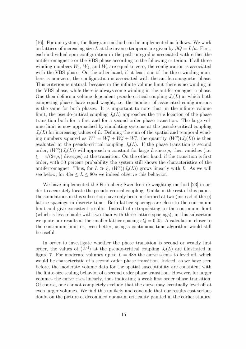
t , the quantity 〈W 2〉(Jc(L)) is thenevaluated at the pseudo-critical coupling Jc(L). If the phase transition is secondorder, 〈W 2〉(Jc(L)) will approach a constant for large L since ρs then vanishes (i.e.ξ = c/(2πρs) diverges) at the transition. On the other hand, if the transition is firstorder, with 50 percent probability the system still shows the characteristics of theantiferromagnet. Thus, for L ≫ ξ, 〈W 2〉(Jc(L)) grows linearly with L. As we willsee below, for 48a ≤ L ≤ 80a we indeed observe this behavior.

We have implemented the Ferrenberg-Swendsen re-weighting method [23] in or-der to accurately locate the pseudo-critical coupling. Unlike in the rest of this paper,the simulations in this subsection have only been performed at two (instead of three)lattice spacings in discrete time. Both lattice spacings are close to the continuumlimit and give consistent results. Instead of extrapolating to the continuum limit(which is less reliable with two than with three lattice spacings), in this subsectionwe quote our results at the smaller lattice spacing εQ = 0.05. A calculation closer tothe continuum limit or, even better, using a continuous-time algorithm would stillbe useful.

In order to investigate whether the phase transition is second or weakly firstorder, the values of 〈W 2〉 at the pseudo-critical coupling Jc(L) are illustrated infigure 7. For moderate volumes up to L = 48a the curve seems to level off, whichwould be characteristic of a second order phase transition. Indeed, as we have seenbefore, the moderate volume data for the spatial susceptibility are consistent withthe finite-size scaling behavior of a second order phase transition. However, for largervolumes the curve rises linearly, thus indicating a weak first order phase transition.Of course, one cannot completely exclude that the curve may eventually level off ateven larger volumes. We find this unlikely and conclude that our results cast seriousdoubt on the picture of deconfined quantum criticality painted in the earlier studies.

15

10 20 30 40 50 60 70 80 90

L/a

3.1

3.2

3.3

3.4

3.5

< W

2 >

Figure 7: The sum of spatial and temporal winding numbers squared 〈W 2〉(Jc(L))evaluated at the pseudo-critical coupling Jc(L) for increasing lattice size L.

L/a 24 32 48 64 80 96

Jc(L)/Q 0.0311(4) 0.0316(3) 0.0337(4) 0.0364(3) 0.0384(3) —J ′

c(L)/Q 0.115(2) 0.0871(4) 0.0632(4) 0.0544(5) 0.0477(4) 0.0445(4)

Table 3: Values of the volume-dependent pseudo-critical couplings Jc(L) and J ′

c(L)obtained with the Ferrenberg-Swendsen re-weighting method.

Given the evidence for a weak first order transition, we like to determine thevalue of the critical coupling Jc in the infinite volume. The values of the pseudo-critical coupling Jc(L) in a finite volume are summarized in table 3. Given thedata for Jc(L) alone, it is non-trivial to extract the infinite volume critical couplingJc = Jc(L→ ∞). For this reason, we have defined another pseudo-critical couplingJ ′

c(L), which also extrapolates to the correct limit, i.e. J ′

c(L → ∞) = Jc. In thiscase, we work at the inverse temperature given by βQ = L/4a. Irrespective of thespatial winding numbers, if the temporal winding number Wt is equal to zero, theconfiguration is now associated with the VBS phase. On the other hand, ifWt is non-zero, the configuration is associated with the antiferromagnetic phase. As before, wedefine the volume-dependent pseudo-critical coupling J ′

c(L) such that both phaseshave equal weight. The values of J ′

c(L) (again quoted at εQ = 0.05) are also listed intable 3. According to the finite-size scaling theory for first order phase transitions,

16

0 0.005 0.01 0.015 0.02 0.025 0.03

a/L

0.03

0.04

0.05

0.06

Figure 8: Fit of the pseudo-critical couplings Jc(L) (lower curve) and J ′

c(L) (uppercurve) shown as functions of a/L.

using βL2 ∝ L3, both finite-volume pseudo-critical couplings should approach theircommon infinite volume limit Jc as

Jc(L) = Jc + ClogL/a

L3, J ′

c(L) = Jc + C ′logL/a

L3. (4.2)

Interestingly, the two pseudo-critical couplings indeed converge to the same limit.A fit of Jc(L) and J

′

c(L) to eq.(4.2) — shown in figure 8 — has χ2/d.o.f. ≈ 1.15 andyields the infinite-volume critical coupling Jc = 0.0396(6). Again, only the large-volume data show the characteristic behavior of a first order phase transition. Itshould be noted that the definition of J ′

c(L) is less natural than the one of Jc(L),because it ignores the spatial winding numbers when configurations are associatedwith either of the two phases. In particular, J ′

c(L) approaches the infinite-volumecritical point Jc more slowly than Jc(L). Consequently, the ultimate large volumephysics is more easily visible using the pseudo-critical coupling Jc(L). For example,the linear increase of 〈W 2〉(Jc(L)) with L, which sets in around L ≈ 50a, is not yetpresent in 〈W 2〉(J ′

c(L)), and is expected to set in only on larger volumes.

17

5 Investigation of the VBS State

As we have seen, the antiferromagnet is weakened and ultimately destroyed at arather weak first order phase transition. Since the transition is so weak, at moderatevolumes it is practically indistinguishable from a continuous transition. As a result,an approximate U(1) symmetry emerges dynamically as an enhancement of thediscrete 90 degrees rotations of the square lattice. The other side of the phasetransition is characterized by VBS order. However, the emergent U(1) symmetrymakes it difficult to identify the nature of the VBS state as columnar or plaquette.

5.1 Probability Distribution of the VBS Order Parameter

In order to investigate the nature of the VBS order it is best to go away from thecritical point as far as possible (assuming that no other phase transitions take place).In the following we thus work at Q/J = ∞, which is obtained by putting J = 0.The corresponding probability distribution of the standard VBS order parametersp(D1, D2) has been determined by Sandvik for a 322 lattice at zero temperature andit shows perfect U(1) symmetry [17]. The loop-cluster algorithm allows us to repeatthis study for larger volumes, in this case using the probability distribution of thenon-standard VBS order parameters p(D1, D2). As one sees from figure 9, even ona 962 lattice at βQ = 30 one does not see any deviation from the U(1) symmetry.Hence, our data do not allow us to identify the nature of the VBS order.

At small Q/J , the loop cluster algorithm is extremely efficient with auto-cor-relations limited to at most a few sweeps. However, at larger values of Q/J , andespecially at Q/J = ∞ the algorithm suffers from a noticeable auto-correlationproblem. This problem arises because the cluster algorithm, which is designed toupdate long-range spin correlations, can not efficiently shuffle spin-flip events fromeven to odd bonds. This causes slowing down in the VBS phase. Details concerningthe algorithm and its performance will be discussed elsewhere.

5.2 Antiferromagnetic Correlations in the VBS Phase

In order to confirm that antiferromagnetism indeed disappears for large Q, we againconsider Q/J = ∞. We have simulated the staggered susceptibility as a function ofthe lattice size L. As one sees in figure 10, at βQ = 50 the staggered susceptibilityχs increases with increasing space-time volume until it levels off around L ≈ 50a.This shows that long (but not infinite) range antiferromagnetic correlations surviveeven deep in the VBS phase. These data confirm that antiferromagnetism is indeeddestroyed in the VBS phase. However, again one needs to go to volumes larger thanL ≈ 50a in order to see the ultimate infinite-volume behavior.

18

Figure 9: Probability distribution p(D1, D2) obtained on a 962 lattice at βQ = 30 andQ/J = ∞. The observed U(1) rotation symmetry implies that we cannot identifythe nature of the VBS phase as either columnar or plaquette.

20 40 60 80

L/a

10

20

30

40

50

χ S J

a

Figure 10: The staggered susceptibility χs in the VBS phase increases with increasingspace-time volume until it levels off around L/a ≈ 50 for βQ = 50.

19

6 Conclusions

We have employed a rather efficient loop-cluster algorithm to investigate the physicsof the antiferromagnetic spin 1

2Heisenberg model with an additional four-spin in-

teraction. When the four-spin coupling is sufficiently strong, antiferromagnetism isdestroyed and gives way to a VBS state. While Sandvik’s pioneering study [17] waslimited to zero temperature and moderate volumes, just like the stochastic seriesexpansion method of Melko and Kaul [20], the cluster algorithm allows us to workat non-zero temperatures and large volumes. Using the cluster algorithm and ap-plying the flowgram method of Kuklov, Prokof’ev, Svistunov, and Troyer [16], wefound numerical evidence for a weak first order phase transition, thus supporting theGinzburg-Landau-Wilson paradigm. Interestingly, the same conclusion was reachedin studies of the transition separating superfluidity from VBS order [14, 15, 16].The first order nature of the phase transition in the Heisenberg model with four-spin coupling Q implies that the idea of deconfined quantum criticality again lacksa physical system for which it is firmly established. Hence, the proponents of thisintriguing idea are challenged once more to suggest another microscopic system forwhich one expects this fascinating phenomenon to occur.

It is interesting to ask why the phase transition separating antiferromagnetismfrom VBS order is so weakly first order. There must be a reason for the longcorrelation length, around 50a, even if it does not go to infinity. Perhaps, the ideasbehind deconfined quantum criticality may still explain this behavior.

Acknowledgements

We have benefited from discussions with F. Niedermayer and M. Troyer. The workof S. C. was supported in part by the National Science Foundation under grantnumber DMR-0506953. We also acknowledge the support of the SchweizerischerNationalfonds.

References

[1] H. G. Evertz, G. Lana, and M. Marcu, Phys. Rev. Lett. 70 (1993) 875.

[2] U.-J. Wiese and H.-P. Ying, Z. Phys. B93 (1994) 147.

[3] B. B. Beard and U.-J. Wiese, Phys. Rev. Lett. 77 (1996) 5130.

[4] S. Chakravarty, B. I. Halperin, and D. R. Nelson, Phys. Rev. B39 (1989) 2344.

[5] H. Neuberger and T. Ziman, Phys. Rev. B39 (1989) 2608.

20

[6] D. S. Fisher, Phys. Rev. B39 (1989) 11783.

[7] P. Hasenfratz and H. Leutwyler, Nucl. Phys. B343 (1990) 241.

[8] P. Hasenfratz and F. Niedermayer, Phys. Lett. B268 (1991) 231.

[9] P. Hasenfratz and F. Niedermayer, Z. Phys. B92 (1993) 91.

[10] M. Greven et al., Phys. Rev. Lett. 72 (1994) 1096; Z. Phys. B96 (1995) 465.

[11] T. Sentil, A. Vishwanath, L. Balents, S. Sachdev, and M. P. A. Fisher, Science303 (2004) 1490; Phys. Rev. B70 (2004) 144407.

[12] O. Motrunich and A. Vishwanath, Phys. Rev. B70 (2004) 075104.

[13] R. K. Kaul, A. Kolezhuk, M. Levin, S. Sachdev, and T. Senthil, Phys. Rev.B75 (2007) 235122.

[14] R. G. Melko, A. W. Sandvik, and D. J. Scalapino, Phys. Rev. B69 (2004)100408(R).

[15] A. Kuklov, N. Prokof’ev, and B. Svistunov, Phys. Rev. Lett. 93 (2004) 230402.

[16] A. Kuklov, N. Prokof’ev, B. Svistunov, and M. Troyer, Annals of Phys. 321(2006) 1602.

[17] A. W. Sandvik, Phys. Rev. Lett. 98 (2007) 227202.

[18] A. W. Sandvik, Phys. Rev. Lett. 95 (2005) 207203.

[19] A. W. Sandvik and K. S. D. Beach, arXiv:0704.1469.

[20] R. G. Melko and R. K. Kaul, arXiv:0707.2961.

[21] K. Harada, N. Kawashima, and M. Troyer, J. Phys. Soc. Jpn. 76 (2007) 013703.

[22] T. Grover and T. Senthil, Phys. Rev. Lett. 98 (2007) 247202.

[23] A. M. Ferrenberg and R. H. Swendsen, Phys. Rev. Lett. 61 (1988) 2635.

21