From the SQL loving folks at - Amazon S3 for faster queries. Some of our most popular blog posts are about speeding up SQL and they consistently ... lazy-analysts-guide

From the SQL loving folks at:

selectdashboards.name,dashboards.name,log_counts.ct from dashboards log_countsfrom dashboards join (select distinc distinct_logs.dashboard_id, count(1) as ctfrom ( select distinct dashboard_id,user_id fromtime_on_site_ as distinct_logs group by distinct_logs.daselectdashboards.name,dashboards.name,log_counts.ct from dashboards log_countsfrom dashboards join (select distinc distinct_logs.dashboard_id, count(1) as ctfrom ( select distinct dashboard_id,user_id fromtime_on_site_ as distinct_logs group by distinct_logs.da nct_logs.daselectdashboards.name,dashboards.name,log_counts.ct from dashboards log_countsfrom dashboards join (select distinc distinct_logs.dashboard_id, count(1) as ctfrom ( select distinct dashboard_id,user_id fromtime_on_site_ as distinct_logs group by distinct_logs.da nct_logs.daselectdashboards.name,dashboards.name,log_counts.ct from


Table of ContentsAbout Periscope and Authors ..............................................

Introduction ...................................................................

Pre-Aggregated Data ........................................................

Reducing Your Data Set ....................................................

Materialized Views ..........................................................

Avoiding Joins ................................................................

Generate_series ............................................................

Window Functions ..........................................................

Avoiding Table Scans ........................................................

Adding an Index ............................................................

Moving Math in Where Clauses ...........................................

Approximations ..............................................................

Hyperloglog ................................................................

Sampling ...................................................................

Thanks for Reading! ........................................................

1

2

3

3

4

6

6

7

9

9

10

11

11

14

16



Page 1

About PeriscopeData analysts all over the world use Periscope to get and share insights fast. Our focus on the people actually running the queries means you get a full featured SQL editor that makes writing sophisticated queries quick and easy.

With our in-memory data caching system, customers realize an average of 150X improvement in query speeds. Our intuitive sharing features allow you to quickly share data throughout your organization. Just type SQL and get charts.

Periscope is built by a small team of hackers working out of a loft in San Francisco. We love our customers, SQL, and that moment when a blip in the data makes you say, "wait a minute…"

Jason Freidman

After leaving Google to join Periscope, Jason promptly began rebuilding Periscope's backend services in Go. Before Google, Jason was lord of backend engineering at SF-based startup Tokbox.

David Ganzhorn

Ganz joined Periscope from Google, where he ran dozens of A/B tests on the search results page, generating billions in new revenue. At Periscope he hacks on all levels of the stack.

Tom O'Neill

Periscope was started in Tom's apartment, where he built the first version of the product in a weekend. He leads Periscope's engineering efforts, and holds the coveted customer-facing bugfix record. (10 minutes!)

Harry Glaser

Harry handles Periscope's customer support, sales, office hunting, whiskey buying, and website copywriting. In his spare time he still checks in a little code, much to the annoyance of the other engineers.

The Authors



IntroductionWe’re All About SQL at Periscope

At Periscope we spend a lot of time working with SQL. Our product is built around creating charts through SQL queries. Every day we help customers write and debug SQL. We’re on a mission to create the world’s best SQL editor. Even our blog is all about SQL!

Why We Made This Book

As part of all this SQL work, we are constantly thinking about how to make our queries faster. One of the most common problems our customers encounter is slow SQL queries. Since they come to us for help, we’ve built a lot of expertise around optimizing SQL for faster queries.

Some of our most popular blog posts are about speeding up SQL and they consistently get positive responses from the community. We figured people must be eager to learn more about it, so we made this ebook hoping it'd be a useful tool for SQL analysts.

What’s in This Book

This book is divided into four sections: Pre-aggregated Data, Avoiding Joins, Avoiding Table Scans and Approximations. Each section has tips that we’ve either covered on our blog or written exclusively for this ebook. The tactics here vary from beginner to advanced: There’s something for everyone!

Now go forth and make your queries faster!

Hugs and queries,

The Periscope Team

Page 2



Page 3

It’s common when running reports to need to combine data for a query from different tables. Depending on where you do this in your process, you can be looking at a severely slow query. At the simplest form an aggregate is a simple summary table that can be derived by performing a group by SQL query.

Aggregations are usually precomputed, partially summarized data, stored in new aggregated tables. The most ideal point to aggregate data for faster queries is aggregating as early in the query as possible.

In this section we’ll go over reducing a data set, grouping data, and materialized views.

Pre-Aggregating Data

For starters, let's assume the handy indices on user_id and dashboard_id are in place, and there are lots more log lines than dashboards and users.

On just 10 million rows, this query takes 48 seconds. To understand why, let's consult our handy SQL explain:

Reducing Your Data Set Count distinct is the bane of SQL analysts, so it was an obvious choice for demonstrating aggregating and reducing your data set. Let's start with a simple query we run all the time: Which dashboards do most users visit?

In Periscope, this would give you a graph like this:

It's slow because the database is iterating over all the logs and all the dashboards, then joining them, then sorting them, all before getting down to real work of grouping and aggregating.

Aggregate, Then Join

Anything after the group-and-aggregate is going to be a lot cheaper because the data size is much smaller. Since we don't need dashboards.name in the group-and-aggregate, we can have the database do the aggregation first, before the join:



Page 4

Materialized viewsThe best way to make your SQL queries run faster is to have them do less work, and a great way to do less work is to query a materialized view that's already done the heavy lifting.

Materialized views are particularly nice for analytics queries. For one thing, many queries do math on the same basic atoms. For another, the data changes infrequently (often as part of daily ETLs). Finally, those ETL jobs provide a convenient home for view creation and maintenance.

Redshift doesn't yet support materialized views out of the box, but with a few extra lines in your import script (or a tool like Periscope), creating and maintaining materialized views as tables is a breeze.

Lifetime Daily ARPU (average revenue per user) is common metric and often takes a long time to compute. Let's speed it up with materialized views.


This query runs in 20 seconds, a 2.4X improvement! Once again, our trusty explain will show us why:

As promised, our group-and-aggregate comes before the join. And, as a bonus, we can take advantage of the index on the time_on_site_logs table.

First, Reduce The Data Set

We can do better. By doing the group-and-aggregate over the whole logs table, we made our database process a lot of data unnecessarily. Count distinct builds a hash set for each group — in this case, each dashboard_id — to keep track of which values have been seen in which buckets.

And now for the big reveal: This query takes 0.7 seconds! That's a 28X increase over the previous query, and a 68X increase over the original query.

As always, data size and shape matters a lot. These examples benefit a lot from a relatively low cardinality. There are a small number of distinct (user_id, dashboard_id) pairs compared to the total amount of data. The more unique pairs there are — the more data rows that must be grouped and counted separately — the less opportunity there is for easy speedups.

Next time count distinct is taking all day, try a few subqueries to lighten the load.

Calculating Lifetime Daily ARPU

This common metric shows the changes in how much money you're making per user over the lifetime of the your product.

We've taken the inner count-distinct-and-group and broken it up into two pieces. The inner piece computes distinct (dashboard_id, user_id) pairs. The second piece runs a simple, speedy group-and-count over them. As always, the join is last.



Page 5

Do the same thing for lifetime_gameplays, and and calculating Lifetime Daily ARPU now takes less than a second to complete!

Remember to drop and recreate these tables every time you upload data to your Redshift cluster to keep them fresh. Or create views in Periscope instead, and we'll keep them up to date automatically!


For that we'll need a purchases table and a gameplays table, and the lifetime accumulated values for each date. Here's the SQL for calculating lifetime gameplays:

That's a monster query and it takes minutes to run on a database with 2B gameplays and 3M purchases. That's way to slow, especially if we want to quickly slice by dimensions like what platform the game was played on. Plus, similar lifetime metrics will need to recalculate the same data over and over again!

Easy View Materialization on Redshift

Conveniently, we wrote our query in a format that makes it obvious which parts can be extracted into materialized views: lifetime_gameplays and lifetime_purchases.

We'll fake view materialization in Redshift by creating tables, and Redshift makes it easy to create tables from snippets of SQL:

The range join in the correlated subquery lets us recalculate the distinct number of users for each date.

Here's the SQL for lifetime purchases in the same format:

Now that the setup is done, we can calculate lifetime daily ARPU:



Page 6

Depending on how your database scheme is structured, you’re likely to have data required for common analysis queries in different tables. Joins are typically used to combine this data. They’re a powerful tool, yet they do have their downside.

Your database has to scan each table that’s joined and figure how each row matches up. This makes joins expensive when it comes to query performance. You can mitigate this through smart join usage, but your queries would be even faster if you could completely avoid joins.

In this section, we’ll go over avoiding joins by using generate_series and window functions.

Avoiding Joins

We can see that iOS is our fastest-growing platform, quickly surpassing the others in lifetime players despite being launched months later!

However, metrics like these can be incredibly slow, since they're typically calculated with distinct counts over asymmetric joins. We'll show you how to calculate these metrics in milliseconds instead of minutes.

Self-Joining

The easiest way to write the query is to join gameplays onto itself. The first gameplays, which we name dates, provides the dates that will go on our X axis. The second gameplays, called plays, supplies every game play that happend on or before each date.

The SQL is nice and simple:

Generate SeriesCalculating Lifetime Metrics

Lifetime metrics are a great way to get a long-term sense of the health of business. They're particularly useful for seeing how healthy a segment is by comparing to others over the long term.

For example, here's a fictional graph of lifetime game players by platform:



Page 7

Window FunctionsEvery user started playing on a particular platform on one day. Once they started, they count forever. So let's start with the first gameplay for each user on each platform:

Avoiding Joins

This query has miserable performance: 37 minutes on a 10,000-row table!

To see why, let's look at our explain:

By asymmetrically joining gameplays to itself, we're bogging down in an n^2 loop. Then we're sorting the whole blown-out table!

Generate Series

Astute readers will notice that we're only using the first gameplays table in the join for its dates. It conveniently has the exact dates we need for our graph — the dates of every gameplay — but we can select those separately and then drop them into a generate_series.

The resulting SQL is still pretty simple:

Don't be fooled by the scans at the top. Those are just to get the single min and max values for generate_series.

Notice that instead of joining and nested-looping over gameplays multiplied by gameplays, we are joining with gameplays and a Postgres function, in this case gener-ate_series. Since the series has only one row per date, the result is a lot faster to loop over and sort.

But we can still do a lot better.

Now that we have that, we can aggregate it into how many first gameplays there were on each platform on each day:

We've included each user's first gameplay per platform in a with clause, and then simply counted the number of users for each date and platform.

Now that we have the data organized this way, we can simply sum the values for each platform over time to get the lifetime numbers! Because we need each date's sum to include previous dates but not new dates, and we need the sums to be separate by platform, we'll use a window function.

This query runs in 26 seconds, achieving an 86X speedup over the previous query!

Here's why:



Page 8

Avoiding Joins

Here's the full query:

The window function is worth a closer look:

As a result, this version runs in 28 milliseconds, a whopping 928X speedup over the previous version, and an unbelievable 79,000X speedup over the original self-join. Window functions to the rescue!

No joins at all! And when we're sorting, it's only over the relatively small daily_first_gameplays with-clause, and the final aggregated result.

Partition by platform means we want a separate sum for each platform. order by dt specifies the order of the rows, in this case by date. That's important because rows between unbounded preceding and current row specifies that each row's sum will include all previous rows (e.g. all previous dates), but no future rows. Thus it becomes a rolling sum, which is exactly what we want.

With the full query in hand, let's look at the explain:



Page 9

Most SQL queries that are written for analysis without performance in mind will cause the database engine to look at every row in the table. After all, if you want to aggregate rows that meet certain conditions, what better way than to see whether each row meets those conditions!

Unfortunately, as datasets get bigger, looking at every single row just won't work in a reasonable amount of time. This is where it helps to give the query planner the tools it needs to only look at a subset of the data. This section will give you a few building blocks that you can use in queries that are scanning more rows than they should.

Avoiding Table Scans

This query takes 74.7 seconds. We can see why by asking Postgres to explain the query:The Power of Indices

Most conversations about SQL performance begin with indices, and rightly so. They possess a remarkable combination of versatility, simplicity and power. Before proceeding with many of the more sophisticated techniques in this book, it's worth understanding what they are and how they work.

Table Scans

Unless otherwise specified, the table is stored in the order the rows were inserted. Unfortunately, this means that queries that only use a small subset of the data – for example, queries about today's data – must still scan through the entire table looking for today's rows.

As an example, let's look at a real-world query. Let's look at today's activity by hour, as measured by the pings table we log events to:

Placeholder

The operation on the left-hand side of the arrow is a full scan of the pings table! Because the table is not sorted by created_at, we still have to look at every row in the table to decide whether the ping happened today or not.

Indexing the data

Let's improve things by adding an index on created_at:

This will create a pointer to every row, and sort those points by the columns we're indexing on – in this case, created_at. The exact structure used to store those pointers depends on your index type, but binary trees are very popular for their versatility and log(n) search times.



Page 10

Avoiding Table Scans

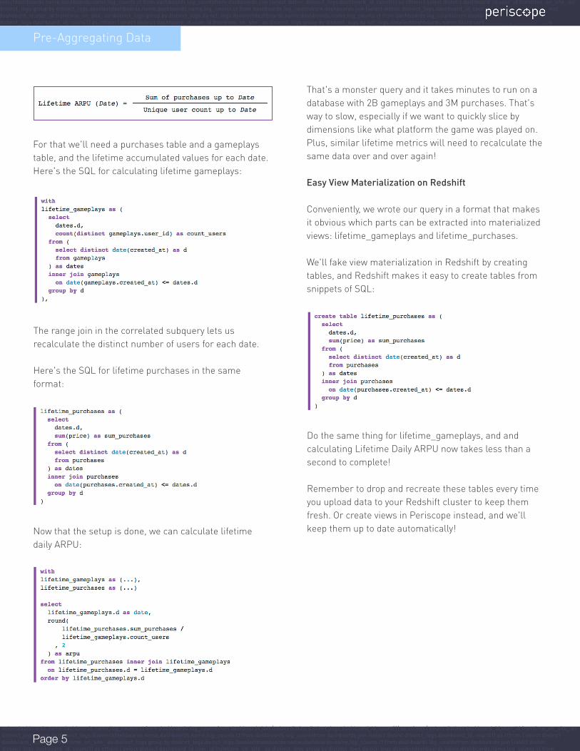
Now that we have an index, let's take a look at how the query works:

Instead of scanning the whole table, we just search the index! To top it off, now that it can ignore the pings that didn't happen today, the query runs in 1.7s – a 44X improvement!

Caveats

Creating a lot of indices on a table will slow down inserts on that table. This is because every index has to be updated every time data is inserted. So proceed with care! A good strategy is to take a look at your most common queries, and create indices designed to maximize efficiency on those queries.

Moving Math in Where ClausesA Deceptively Simple Query

Front and center on our Periscope dashboard is a question we ask all the time: How much usage has there been today?

To answer it, we've written a seemingly simple query:

Ignoring The Index

As usual, running explain will tell us why it's slow: It turns out our database is ignoring the index and doing a sequential scan!

The problem is that we're doing math on our indexed column, created_at. This causes the database to look at each row in the table, compute created_at - interval '8 hour' for that row, and compare the result to date(now() - interval '8 hour').

Moving Math To The RHS

Our goal is to compute one value in advance, and let the database search the created_at index for that value. To do that, we can just move all the math to the right-hand-side of the comparison:

This query runs in a blazing 85ms. With a simple change, we've achieved a 3,000X speedup!

As promised, with a single value computed in advance, the database can search its index:

Of course, sometimes the math can't be refactored quite so easily. But when writing queries with restricts on indexed columns, avoid math on the indexed column. You can get some pretty massive speedups.

Notice the "- interval '8 hour'" operations in the where clause. Times are stored in UTC, but we want "today" to mean today PST.

As the time_on_site_logs table has grown to 22M rows, even with an index on created_at, this query has slown way down to an average of 267 seconds!



Page 11

For truly large data sets, approximations can be one of the most powerful performance tools in your toolset. In certain contexts, an answer that is accurate to +/- 5% is just as useful for making a decision and multiple orders of magnitude faster to get.

More than most techniques, this one comes with a few caveats. The first is making sure the customers of your data understand the limitations. Error bars are a useful visualization that are well-understood by data consumers.

The second caveat is to understand the assumptions your technique makes about the distribution of your data. For example, if your data isn't normally distributed, sampling is going to produce incorrect results.

For more details about various technique and their uses, read on!

Approximations

When there there are too many elements to fit in RAM, the database writes them to disk, sorts the file, and then counts the number of element groups. The second case — writing the intermediate data to disk — is very slow. Probabilistic counters are designed to use as little RAM as possible, making them ideal for large data sets that would otherwise page to disk.

HyperloglogWe'll optimize a very simple query, which calculates the daily distinct sessions for 5,000,000 gameplays (~150,000/day):

The original query takes 162.2s. The HyperLogLog version is 5.1x faster (31.5s) with a 3.7% error, and uses a small fraction of the RAM.

Why HyperLogLog?

Databases often implement count(distinct) in two ways: When there are few distinct elements, the database makes a hashset in RAM and then counts the keys.

The HyperLogLog Probabilistic Counter is an algorithm for determining the approximate number of distinct elements in a set using minimal RAM. Distincting a set that has 10 million unique 100-character strings can take over gigabyte of RAM using a hash table, while HyperLogLog uses less than a megabyte (the "log log" in HyperLogLog refers to its space efficiency). Since the probabilistic counter can stay entirely in RAM during the process, it's much faster than any alternative that has to write to disk and usually faster than alternatives using a lot more RAM.



Page 12

Approximations

Hashing

The core of the HyperLogLog algorithm relies on one simple property of uniform hashes: The probability of the position of the leftmost set bit in a random hash is 1/2n, where n is the position. We call the position of the leftmost set bit the most significant bit, or MSB.

Here are some hash patterns and the positions of their MSBs:

We'll use the MSB position soon, so here it is in SQL:

Bucketing

The maximum MSB for our elements is capable of crudely estimating the number of distinct elements in the set. If the maximum MSB we've seen is 3, given the probabilities above we'd expect around 8 (i.e. 23) distinct elements in our set. Of course, this is a terrible estimate to make as there are many ways to skew the data.

The HyperLogLog algorithm divides the data into evenly-sized buckets and takes the harmonic mean of the maximum MSBs of those buckets. The harmonic mean is better here since it discounts outliers, reducing the bias in our count.

Using more buckets reduces the error in the distinct count calculation, at the expense of time and space. The function for determining the number of buckets needed given a desired error is:

We'll aim for a +/- 5% error, so plugging in 0.05 for the error rate gives us 512 buckets. Here's the SQL for grouping MSBs by date and bucket:

The hashtext(...) & (512 - 1) gives us the rightmost 9 bits, 511 in binary is 111111111), and we're using that for the bucket number.

The bucket_hash line uses a min inside the logarithm instead of something like this max(31 - floor(log(...))) so that we can compute the logarithm once - greatly speeding up the calculation.

Now we've got 512 rows for each date - one for each bucket - and the maximum MSB for the hashes that fell into that bucket. In future examples we'll call this select bucketed_data.

Hashtext is an undocumented hashing function in postgres. It hashes strings to 32-bit numbers. We could use md5 and convert it from a hex string to an integer, but this is faster.

We use ~(1 << 31) to clear the leftmost bit of the hashed number. Postgres uses that bit to determine if the number is positive or negative, and we only want to deal with positive numbers when taking the logarithm.

The floor(log(2,...)) does the heavy lifting: The integer part of base-2 logarithm tells us the position (from the right) of the MSB. Subtracting that from 31 gives us the position of the MSB from the left, starting at 1.

With that line we've got our MSB per-hash of the session_id field!



Page 13

Approximations

Counting

It's time to put together the buckets and the MSBs. The paper linked above has a lengthy discussion on the derivation of this function, so we'll only recreate the result here. The new variables are m (the number of buckets, 512 in our case) and M (the list of buckets indexed by j, the rows of SQL in our case). The denomina-tor of of this equation is the harmonic mean mentioned earlier:

In SQL, it looks like this:

And the SQL for that looks like this:

Now putting it all together:

And that's the HyperLogLog probabilistic counter in pure SQL!

Bonus: Parallelizing

The HyperLogLog algorithm really shines when you're in an environment where you can count distinct in parallel. The results of the bucketed_data step can be combined from multiple nodes into one superset of data, greatly reducing the cross-node overhead usually required when counting distinct elements across a cluster of nodes. You can also preserve the results of the bucketed_data step for later, making it nearly free to update the distinct count of a set on the fly!

We add in (512 - count(1)) to account for missing rows. If no hashes fell into a bucket it won't be present in the SQL, but by adding 1 per missing row to the result of the sum we achieve the same effect.

The num_zero_buckets is pulled out for the next step where we account for sparse data.

Almost there! We have distinct counts that will be right most of the time - now we need to correct for the extremes. In future examples we'll call this select counted_data.

Correcting

The results above work great when most of the buckets have data. When a lot of the buckets are zeros (missing rows), then the counts get a heavy bias. To correct for that we apply the formula below only when the estimate is likely biased, with this equation:



Page 14

Approximations

SamplingSampling is an incredibly powerful tool to speed up analyses at scale. While it's not appropriate for all datasets or all analyses, when it works, it really works. At Periscope, we've realized several orders of magnitude in speedups on large datasets with judicious use of sampling.

However, when sampling from databases, it's easy to lose all your speedups by using inefficient methods to select the sample itself. In this post we'll show you how to select random samples in fractions of a second.

The Obvious, Correct, Slow solution

Let's say we want to send a coupon to a random hundred users as an experiment. Quick, to the database!

The naive approach sorts the entire table randomly and selects N results. It's slow, but it's simple and it works even when there are gaps in the primary keys.

Selecting a random row:

The database is sorting the entire table before selecting our 100 rows! This is an O(n log n) operation, which can easily take minutes or longer on a 100M+ row table. Even on medium-sized tables, a full table sort is unacceptably slow in a production environment.

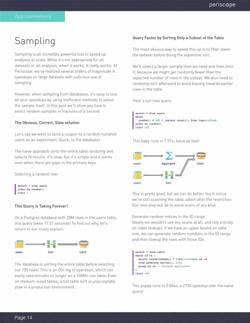
Query Faster by Sorting Only a Subset of the Table

The most obvious way to speed this up is to filter down the dataset before doing the expensive sort.

We'll select a larger sample than we need and then limit it, because we might get randomly fewer than the expected number of rows in the subset. We also need to randomly sort afterward to avoid biasing towards earlier rows in the table.

Here's our new query:

This baby runs in 7.97s: twice as fast!

This is pretty good, but we can do better. You'll notice we're still scanning the table, albeit after the restriction. Our next step will be to avoid scans of any kind.

Generate random indices in the ID rangeIdeally we wouldn't use any scans at all, and rely entirely on index lookups. If we have an upper bound on table size, we can generate random numbers in the ID range and then lookup the rows with those IDs.

This puppy runs in 0.064s, a 273X speedup over the naive query!

This Query is Taking Forever!

On a Postgres database with 20M rows in the users table, this query takes 17.51 seconds! To find out why, let's return to our trusty explain:



Page 15

Approximations

Counting the table itself takes almost 8 seconds, so we'll just pick a constant beyond the end of the ID range, sample a few extra numbers to be sure we don't lose any, and then select the 100 we actually want.

Bonus: Random sampling with replacement

Imagine you want to flip a coin a hundred times. If you flip a heads, you need to be able to flip another heads. This is called sampling with replacement. All of our previous methods couldn't return a single row twice, but the last method was close: If we remove the inner group by id, then the selected ids can be duplicated:

Sampling is an incredibly powerful tool for speeding up statistical analyses at scale, but only if the mechanism for getting the sample doesn't take too long. Next time you need to do it, generate random numbers first, then select those records. Or, try Periscope, which will use sampling to speed up your analyses without any work on your end!



Thanks for Reading!We hope you gained some new tools for your SQL toolbelt. We put a lot of work into our first ebook and hope to put in even more as we expand on our techniques for making SQL faster.

Please email us at [email protected] with any questions or feedback about this ebook, Periscope, or SQL in general. We’d love to hear from you!

Shameless Plug Alert

Looking for a better way to analyze your SQL database data? Want your queries to run faster? Want to make sharing reports across your business easy?

Thousands of analysts use Periscope every day to dig deeper into their data and find the insights they need to grow their business.

Customers realize an average of 150X improvement in query speeds with our preemptive data cache. Even our world class support is fast, with an average response time of 6 seconds during business hours.

Head to Periscope.io and sign up to get started with our 7 day free trial.

This is Just the Beginning

There are a number of techniques for optimizing queries that we didn’t cover here. We have a lot of ideas that didn’t fit in the first version, but that we’re excited to get out over the following months.

Want to be kept up to date on our ebook updates? Sign up at periscope.io/optimizing-sql to get on the mailing list and hear about all the ways we’re improving the guide.

Page 16

Documents

From the SQL loving folks at - Amazon S3 for faster queries. Some of our most popular blog posts are about speeding up SQL and they consistently ... lazy-analysts-guide