From the Hartree dynamics to the Vlasov equation

Niels Benedikter, Marcello Porta, Chiara Saffirio and Benjamin Schlein

December 27, 2015

Abstract

We consider the evolution of quasi-free states describing N fermions in the mean field limit,as governed by the nonlinear Hartree equation. In the limit of large N , we study the convergencetowards the classical Vlasov equation. For a class of regular interaction potentials, we establishprecise bounds on the rate of convergence.

1 Introduction and main results

This work is motivated by the study of the time-evolution of systems of N fermions in the mean fieldregime, characterized by a large number of weak collisions. The many body evolution of N fermionsis generated by the Hamilton operator

HN =

N∑j=1

−∆xj + λ

N∑i<j

V (xi − xj) (1.1)

acting on

L2a(R3N ) = {ψ ∈ L2(R3N ) : ψ(xπ1, . . . , xπN ) = σπψ(x1, . . . , xN ) for all π ∈ SN},

the subspace of permutation antisymmetric functions in L2(R3N ) (σπ denotes here the sign of thepermutation π). Due to the antisymmetry, the kinetic energy in (1.1) is typically (for data occupyinga volume of order one) of the order N5/3 (for bosons, particles described by permutation symmetricwave functions, it is much smaller, of order N). Hence, to obtain a non-trivial competition betweenkinetic and potential energy, we have to choose λ = N−1/3. Moreover, the large kinetic energy of theparticles implies that we can only follow their time evolution for short times, of the order N−1/3 (thekinetic energy per particle is proportional to N2/3; the typical velocity of the particles is therefore ofthe order N1/3). After rescaling time, the evolution of the N fermions is governed by the many bodySchrodinger equation

iN1/3∂tψN,t =

N∑j=1

−∆xj +1

N1/3

N∑i<j

V (xi − xj)

ψN,t (1.2)

for ψN,t ∈ L2a(R3N ). It is convenient to rewrite (1.2) as follows. We introduce the small parameter

ε = N−1/3

1

and we multiply (1.2) by ε2. We obtain

iε∂tψN,t =

N∑j=1

−ε2∆xj +1

N

N∑i<j

V (xi − xj)

ψN,t . (1.3)

Hence, the mean field scaling for fermionic systems (characterized by the N−1 factor in front of thepotential energy) is naturally linked with a semiclassical scaling, where ε = N−1/3 plays the role ofPlanck’s constant. Notice that for particles in d dimensions, similar arguments show that we wouldhave to take ε = N−1/d; in fact, our analysis applies to general dimensions (with appropriate changeson the regularity assumptions); to simplify our presentation we will only discuss the case d = 3.

From the point of view of physics, we are interested in understanding the evolution of the fermionicsystem resulting from a change of the external fields. In other words, we are interested in the solutionof (1.3) for initial data describing equilibrium states of trapped systems. It is expected (and in certaincases, it is even known) that equilibrium states in the mean-field regime are approximately quasi-free.

At zero temperature, the relevant quasi-free states are Slater determinants, having the form

ψSlater(x1, . . . , xN ) =1√N !

det (fj(xi))1≤i,j≤N

where {fj}Nj=1 is an orthonormal system in L2(R3). Slater determinants are completely characterized

by their one-particle reduced density ωN , defined as the non-negative trace class operator over L2(R3)with the integral kernel

ωN (x; y) = N

∫dx2 . . . dxN ψSlater(x, x2, . . . , xN )ψSlater(y, x2, . . . , xN ) .

A simple computation shows that

ωN =

N∑j=1

|fj〉〈fj | ,

i.e. ωN is the orthogonal projection onto the N -dimensional space spanned by the N orbitals f1, . . . , fNdefining ψSlater (we used here the notation |f〉〈f | to indicate the orthogonal projection onto f ∈L2(R3)). In the language of probability theory, the one-particle reduced density corresponds to theone-particle marginal distribution, obtained by integrating out the degrees of freedom of the other(N − 1) particles. Slater determinants have the properties that higher order marginals can all beexpressed in terms of ωN via the Wick rule (this is, in fact, the defining property of quasi-free states).

The many-body evolution of a Slater determinant, as determined by (1.3), is not a Slater determi-nant. Still, because of the mean-field form of the interaction, we can expect it to remain close, in anappropriate sense, to a Slater determinant. Under this assumption, it is easy to find a self-consistentequation for the dynamics of the Slater determinant. We obtain the nonlinear Hartree-Fock equation

iε∂tωN,t =[−ε2∆ + (V ∗ ρt)−Xt, ωN,t

]. (1.4)

Here ρt(x) = N−1ωN (x;x) is the normalized density of particles at x ∈ R3, the exchange operator Xt

has the integral kernel Xt(x; y) = N−1V (x − y)ωN,t(x; y), and, as before, ε = N−1/3. It is easy tocheck that, if ωN,t=0 is an orthogonal projection with rank N , then the same is true for the solutionωN,t; in other words, the Hartree-Fock evolution of a Slater determinant is again a Slater determinant.

2

In [7], it was shown that indeed, for sufficiently regular interaction potentials, the many bodySchrodinger evolution of initial Slater determinants can be approximated by the Hartree-Fock evo-lution, in the sense that the one-particle reduced density associated with the solution ψN,t of (1.3)remains close (in the Hilbert-Schmidt and in the trace norm) to the solution ωN,t of the Hartree-Fockequation (1.4). Previous results in this direction have been obtained in [9]; convergence towards theHartree-Fock dynamics in other regimes, which do not involve a semiclassical limit, has been alsoestablished in [5, 10, 18, 4].

At positive temperature, on the other hand, relevant quasi-free states approximating equilibria oftrapped systems are mixed states, described by a one-particle reduced density ωN with trωN = N and0 ≤ ωN ≤ 1 (it follows from the Shale-Stinespring condition, see e. g. [20, Theorem 9.5], that everysuch ωN is the one-particle reduced density of a quasi-free state with N particles; Slater determinantsform a special case, with ωN having only the eigenvalues 0 and 1). In the simple case of N fermionswith one-particle Hamiltonian h = −ε2∆ +Vext and no interaction, equilibrium at temperature T > 0is described by the Gibbs state with one-particle reduced density

ωN =1

1 + e1T

(−ε2∆+Vext−µ)(1.5)

where the chemical potential µ ∈ R has to be chosen so that trωN = N . If we turn on a mean-fieldinteraction, it is expected that equilibrium states continue to be approximated by quasi-free stateswith one-particle reduced density of the form (1.5), with the external potential Vext appropriatelymodified to take into account, in a self-consistent manner, the interaction among the particles (forresults in this direction see, for example, [16, 19]).

In suitable scaling regimes, the state of the system at positive temperature is expected to be wellapproximated by an appropriate mixed quasi-free state. Similarly as in the case of Slater determinants,mixed quasi-free states are completely characterized by their one-particle reduced density. All higherorder correlation functions (i.e. all higher order marginals) can be expressed in terms of ωN

1. For theevolution of mixed quasi-free states, we find the same self-consistent equation (1.4) derived for Slaterdeterminants. We observe here that the properties trωN = N and 0 ≤ ωN ≤ 1, characterizing thereduced one-particle density of mixed quasi-free states, are preserved by the Hartree-Fock equation(1.4). In [6], it was shown that, for sufficiently regular potential, the many-body evolution of a mixedquasi-free state can be approximated by the self-consistent Hartree-Fock equation (1.4) (also here, theconvergence has been established through bounds on the distance between reduced densities).

To summarize, it follows from the analysis of [7, 6] that the many-body evolution of fermionicquasi-free states can be approximated by the Hartree-Fock equation (1.4). This holds true for Slaterdeterminants (in this case ωN,t is an orthogonal projection with rank N) as well as for general mixedquasi-free states (satisfying only trωN,t = N and the bounds 0 ≤ ωN,t ≤ 1).

In the mean field regime, the energy contribution associated with the exchange term can be esti-mated as follows, for bounded potentials V :∣∣∣ 1

2N

∫dxdy V (x− y)|ω(x; y)|2

∣∣∣ ≤ ‖V ‖∞2N

‖ωN‖2HS ≤ C , (1.6)

where the full energy is of order N (here we used that the Hilbert-Schmidt norm2 of ωN is boundedby N1/2). Because of the smallness of the exchange term, instead of considering the Hartree-Fock

1In general quasi-free states are characterized by two operators on L2(R3), a one-particle reduced density ωN and apairing density α. Here we restrict our attention to states with α = 0; this is expected to be a very good approximationfor equilibrium states of fermions in the mean field regime considered here.

2The Hilbert-Schmidt norm of a compact operator A is defined as ‖A‖2HS = trA∗A

3

equation (1.4), we will drop the exchange term and study the fermionic Hartree dynamics, governedby the nonlinear equation

iε∂tωN,t =[−ε2∆ + (V ∗ ρt), ωN,t

](1.7)

with ρt(x) = N−1ωN,t(x;x) (a proof of the fact that the exchange term does not affect the dynamicscan be found in Appendix A of [7]).

The Hartree equation (1.7) still depends on N (recall the choice ε = N−1/3 and the normalizationtrωN = N). It is therefore natural to ask what happens to it in the limit N → ∞. To answer thisquestion, we define the Wigner transform of the one-particle reduced density ωN,t by setting

WN,t(x, v) =( ε

2π

)3∫ωN,t

(x+

εy

2;x− εy

2

)e−iv·ydy . (1.8)

Hence, WN,t is a function of position and velocity, defined on the phase-space R3×R3. It is normalizedso that ∫

WN,t(x, v)dxdv = ε3trωN,t = 1 .

The Wigner transform can be inverted, noticing that

ωN,t(x; y) = N

∫dvWN,t

(x+ y

2, v)eiv·

x−yε . (1.9)

Eq. (1.9) is known as the Weyl quantization of the functionWN,t. Notice that ‖ωN,t‖HS =√N‖WN,t‖2.

The Wigner transform WN,t can be used to compute expectations in the quasi-free state describedby ωN,t of observables depending only on the position x or on the momentum −iε∇ of the particles.In fact, for a large class of functions f on R3,

tr f(x)ωN,t =

∫dxf(x)ωN,t(x;x) = N

∫dvdxf(x)WN,t(x, v)

and

tr f(iε∇)ωN,t = N

∫dxdv f(v)WN,t(x, v)

In other words,∫dvWN,t(x, v) is the density of fermions in position space at point x ∈ R3, while∫

dxWN,t(x, v) is the density of particles with velocity v ∈ R3. Notice, however, that WN,t is nota probability density on the phase-space, because in general it is not positive (this observation isrelated with the Heisenberg principle; position and momentum of the particles cannot be measuredsimultaneously with arbitrary precision).

From (1.7), we find an evolution equation for the Wigner transform WN,t:

iε∂tWN,t(x, v) =1

(2π)3

∫dy iε∂tωN,t

(x+

εy

2;x− εy

2

)e−iv·y

=ε2

(2π)3

∫dy (−∆x+εy/2 + ∆x−εy/2)ωN,t

(x+

εy

2;x− εy

2

)e−iv·y

+1

(2π)3

∫dy ((V ∗ ρt)(x+ εy/2)− (V ∗ ρt)(x− εy/2))ωN,t

(x+

εy

2;x− εy

2

)e−iv·y .

Using −∆x+εy/2 + ∆x−εy/2 = −2/ε∇x · ∇y and expanding

(V ∗ ρt)(x+ εy/2)− (V ∗ ρt)(x− εy/2) ' εy · ∇(V ∗ ρt) +O(ε2)

4

we conclude, formally, that

iε∂tWN,t(x, v) = − 2ε1

(2π)3∇x ·

∫dy∇yωN,t

(x+

εy

2;x− εy

2

)e−iv·ydy

+ ε∇(V ∗ ρt)(x)1

(2π)3

∫dy y ωN,t

(x+

εy

2;x− εy

2

)e−iv·ydy +O(ε2)

= −2iεv · ∇xWN,t(x, v) + iε∇(V ∗ ρt)(x) · ∇vWN,t(x, v) +O(ε2) .

As a consequence, we expect that, in the limit N → ∞ (and hence ε → 0; recall that ε = N−1/3),WN,t approaches a solution Wt of the classical Vlasov equation

∂tWt + 2v · ∇xWt = ∇(V ∗ %t) · ∇vWt (1.10)

with the density %t(x) =∫Wt(x, v)dv (in contrast with WN,t, the limit Wt is a probability density, if

this is true at time t = 0). The goal of this paper is to study the convergence of the Hartree dynamicstowards the Vlasov equation (1.10), in the limit N →∞.

This work is not the first one devoted to the derivation of the Vlasov equation (1.10) from quantumevolution equations. In [15, 21], the Vlasov equation is obtained directly from many body quantumdynamics, starting from the fundamental N -fermion Schrodinger equation (the Vlasov equation alsoemerges in the N -boson case, if the mean field limit is combined with a semiclassical limit; see [12],where the dynamics of factored WKB states is analyzed). In [13, 14], the authors take the Hartreeequation (1.7) as starting point of their analysis, and they prove convergence (in a weak sense) towardsthe solution of the Vlasov equation (1.10). Note that the analysis of [13, 14] also applies to singularinteractions, including a Coulomb potential (the analysis was extended to the Hartree-Fock equationin [11]).

In [15, 21, 13, 14, 11], the convergence towards the classical Vlasov dynamics is established inan abstract sense, without control on its rate. The problem of determining bounds on the rate ofconvergence is not only of academic interest. When considering applications to real physical systems,the number of particles N is large but, of course, finite. Bounds on the rate of convergence are thereforeimportant to decide whether N is large enough for the Vlasov equation to be a good approximationof the Hartree and of the full many body Schrodinger dynamics.

Bounds on the rate of convergence of the Hartree evolution towards the Vlasov equation have beenfirst obtained in [3]. In this paper the authors obtain the convergence in the Hilbert-Schmidt with arelative rate ε2/7 = N−2/21 for sufficiently regular initial data and potentials (they require V ∈ H1(R3)and that V ∈ L1(R3, (1 + |p|4)dp)). For smooth potentials, an expansion of the solution of the Hartreeequation (1.7) in powers of ε has been shown in [17] (with no control on the remainder) and in [1, 2].

Our approach here is similar to the one of [3]; we consider the solution of the Hartree equation(1.7) for initial data ωN with sufficiently smooth Wigner transform WN , and we compare it with theWeyl quantization of the solution of the Vlasov equation (1.10), with initial data WN . We considerregular interaction potentials. In Theorem 2.1 and in Theorem 2.2 we establish bounds on the norm-distance of the solution of the Hartree equation ωN,t with initial data ωN and the Weyl quantizationωN,t of the solution of the Vlasov equation with initial data WN . For every fixed t ∈ R, the relativeerror is of the order ε = N−1/3 in the limit of large N . The dependence on N of these boundsis expected to be optimal. This expectation is confirmed by the expansion of [1], where the nextorder corrections are constructed (in fact, if we assumed initial data with smooth Wigner transformWN ∈ W∞,∞(R3 × R3) and smooth interaction potential V ∈ W∞,∞(R3), the result of Theorem 2.1would follow from Theorem 1.2 in [1]).

5

In Theorem 2.1, we get convergence in the trace-norm, for very regular initial data. In Theorem2.2, we bound the Hilbert-Schmidt norm, under weaker assumptions on the regularity of WN . Thestrategy to show Theorem 2.2 is similar to the one of [3]; we regularize the initial data, we comparethe solutions of the regularized Hartree and Vlasov equations and then we establish stability of bothequations with respect to the regularization. We can improve the bounds of [3] by using the tracenorm convergence shown in Theorem 2.1 for the solutions with regularized data. The nonlinearity inthe Hartree and in the Vlasov equation depends on the convolution of the potential with the densityof particles in space. Differences among densities can be easily controlled through the trace-norm ofthe corresponding fermionic operators (which are bounded in Theorem 2.1). Estimating them directlyby means of Hilbert-Schmidt norms, as done in [3], leads instead to a deterioration of the rate ofconvergence.

Notice that, in Theorems 2.1 and 2.2, we consider the solution of the Vlasov equation for initialdata which are not probability densities. The well-posedness of the Vlasov equation for such initialdata can be obtained adapting the arguments of [8]; in Appendix A we sketch the proof.

If we assume additionally that the sequence of initial data ωN has a limit, in the sense thattheir Wigner transform WN converge towards a probability density W0, then we can also establish theconvergence of the Wigner transform WN,t of the solution of the Hartree equation towards the solutionof the Vlasov equation Wt with initial data W0 (in this case, the solution of the Vlasov equation is aclassical probability density, for all t ∈ R). This is the content of Theorem 2.3.

Our bounds on the norms of the distance between the Wigner transform WN,t and the solution ofthe Vlasov equation Wt (as well as the bounds for the distance between WN,t and the Weyl quantization

WN,t of the solution of the Vlasov equation with initial data WN ) hold for sufficiently regular initialdata. In particular, Theorem 2.2 needs WN ∈ H2(R3×R3) (with some additional weights; see Theorem2.4 for the precise assumptions). This condition is justified for initial data describing equilibrium statesof confined fermionic system at positive temperatures. At zero temperature, on the other hand, thesystem at equilibrium relaxes to its ground state, which can be approximated by a Slater determinant.Typically, in this case, the corresponding Wigner transform is not regular. For example, the groundstate of a system of N free fermions in a periodic box with volume one is a Slater determinant withWigner transform

WN (x, v) = N−11(|v| ≤ cρ1/3) (1.11)

where ρ = N is the density of the particles (this system is translation invariant; therefore, particles areuniformly distributed in the box). Eq. (1.11) corresponds to the idea that to construct the free groundstate, we should fill the N one-particle states with the smallest possible energy (by the antisymmetry offermionic wave functions, there cannot be two particles in the same state). If we switch on an externalpotential and a mean-field interaction, it is believed that the ground state can still be approximatedby a state with Wigner transform of the form (1.11); the only difference is that now we have to filllow energy states locally, according to an effective particle density ρTF that can be determined byminimizing the Thomas-Fermi functional

ETF(ρ) =3

5cTF

∫dx ρ5/3(x) +

∫dxVext(x)ρ(x) +

1

2

∫dxdy V (x− y)ρ(x)ρ(y)

among all ρ ∈ L1∩L5/3(R3) with ‖ρ‖1 = N . The resulting sequence of Wigner transforms WN (x; v) =

N−11(|v| ≤ cρ1/3TF (x)) is not in H2(R3 × R3). So, while Theorem 2.1, Theorem 2.2 and Theorem 2.3

provide a good description of the fermionic dynamics in the mean field limit at positive temperature,they cannot be applied at zero temperature.

6

For such initial data, we do not get norm convergence towards the solution of the Vlasov equation.Nevertheless, in Theorem 2.4 and Theorem 2.5 we can still prove convergence for the expectationof a class of semiclassical observables. Semiclassical observables are functions of the multiplicationoperator x and of the momentum operator −iε∇; they detect variations in the spatial distributionof the particles on “macroscopic” scales of order one and, at the same time, they are sensitive tovariations of order ε−1 in the momentum distribution (corresponding to the “microscopic” lengthscale ε).

Let us stress the fact that, to the best of our knowledge, Theorem 2.4 and Theorem 2.5 are thefirst rigorous results concerning convergence from the Hartree dynamics towards the Vlasov equationthat can be applied to reasonable approximations of ground states.

In Section 2, in the remarks following our main theorems, we provide explicit examples of fermionicstates, constructed with the help of coherent states, approximating ground states and positive tem-perature equilibrium states of fermionic systems in the mean-field regime, to which our theorems canbe applied.

2 Statement of the results

In order to state our results in a precise form, we need to introduce some norms for functions on thephase space (x, v) ∈ R3 × R3. For s ∈ N, we define the Sobolev norm

‖f‖2Hs =∑|β|≤s

∫|∇βf(x, v)|2dxdv

where β is a multi-index, and ∇β can act on both position and momentum variables. For s, a ∈ N, weintroduce also the weighted norms

‖f‖2Hsa

=∑|β|≤s

∫(1 + x2 + v2)a|∇βf(x, v)|2dxdv

We are now ready to state our main theorems. In the first theorem, we assume strong regularityof the initial data, and we prove bounds in the trace-norm.

Theorem 2.1. Let V ∈ W 2,∞(R3). Let ωN be a sequence of reduced densities on L2(R3), withtrωN = N , 0 ≤ ωN ≤ 1 and with Wigner transform WN satisfying ‖WN‖H5

4≤ C, uniformly in N .

We denote by ωN,t the solution of the Hartree equation

i∂tωN,t =[−ε2∆ + (V ∗ ρt), ωN,t

](2.1)

with ρt(x) = N−1ωN,t(x;x) and initial data ωN .

On the other hand, we denote by WN,t the solution of the Vlasov equation

∂tWN,t + 2v · ∇xWN,t = ∇(V ∗ ρt) · ∇vWN,t (2.2)

with ρt(x) =∫dv WN,t(x, v) and with initial data WN,0 = WN . Moreover, let ωN,t be the Weyl

quantization of WN,t, defined as in (1.9).Then there exists a constant C > 0 (depending on ‖V ‖W 2,∞ and on supN ‖WN‖H2

4, but not on the

higher Sobolev norms of WN ) such that

tr |ωN,t − ωN,t| ≤ CNε exp(C exp(C|t|))[1 +

3∑k=1

εk supN‖WN‖Hk+2

4

]. (2.3)

7

Remarks.

1) Recall that we use the normalization trωN,t = N . In this sense, (2.3) shows that ωN,t and ωN,tare close, in the limit of large N , since their difference is smaller, by a factor ε = N−1/3, thantheir trace norms.

2) The assumption ‖WN‖H54≤ C on the Wigner transform of the initial data is equivalent to

suitable commutator estimates for the initial fermionic reduced density ωN with the differentialoperator ∇ and the multiplication operator x. We begin by noticing that

‖∇xWN‖22 =

∫dxdv |∇xWN (x, v)|2

=

∫dxdv

∣∣∣ ε3

(2π)3

∫dy e−iv·y[∇, ωN ](x+ εy/2, x− εy/2)

∣∣∣2= N−1‖[∇, ωN ]‖2HS .

(2.4)

Similarly, we find ‖∇vWN‖22 = N−1ε−2‖[x, ωN ]‖2HS. As for the weights in the definition of theHsa-norms of WN , we notice that

‖(1 + x2 + v2)a/2WN‖22 ≤ CN−1‖(1 + x2 − ε2∆)a/2ωN‖2HS ,

for some N -independent constant C > 0.

Proceeding analogously, one can show that the estimate ‖WN‖H54≤ C follows from the bounds

N−1‖(1 + x2 − ε2∆)a/2[a1, [a2, [a3, [a4, [a5, ωN ]]]]]‖2HS ≤ C , (2.5)

uniformly in N and for all choices of a1, . . . , a5 with either ai = x/ε or ai = ∇.

Therefore the commutator structure allows to quantify the regularity and decay properties ofthe quantum state WN . Estimates of commutators [x, ωN ] and [ε∇, ωN ] already played a keyrole in [6, 7].

3) The estimate supN ‖WN‖H54≤ C or, equivalently, the bounds (2.5), are expected to hold true for

fermionic mixed states, describing systems of N particles in equilibrium at positive temperature,in the mean-field regime, [6]. A reasonable approximation for the reduced density of such a stateis given by the superposition

ωN (x; y) =

∫dpdrM(r, p)fpr(x)fpr(y) , (2.6)

of the coherent statesfpr(x) = ε−3/2e−ip·x/εg(x− r) (2.7)

with a probability density M with 0 ≤M(r, p) ≤ 1 and∫dpdrM(r, p) = 1

In (2.7), the function g is assumed to vary on the (possibly N -dependent) scale δ and to benormalized so that ‖g‖2 = 1. For simplicity, we shall make the explicit choice

g(x) =1

(2πδ2)3/4e−x

2/2δ2 . (2.8)

8

It is simple to check that, with the definition (2.6), one indeed finds that 0 ≤ ωN ≤ 1 andtrωN = N .

The smoothness and decay properties of the Wigner transform WN of (2.6) follow from analogousproperties of the phase space density M(r, p), i.e.

‖WN‖H54≤ C‖M‖H5

4. (2.9)

In fact, according to the previous remark, to prove (2.9) it is enough to show (2.5). To this end,we notice that

[x/ε, ωN ](x; y) =

∫dpdrM(p, r)(−i∇p)fpr(x)fpr(y) =

∫dpdr (i∇pM(p, r))fpr(x)fpr(y)

[∇, ωN ](x; y) =

∫dpdrM(p, r)∇rfpr(x)fpr(y) = −

∫dpdr (∇rM(p, r))fpr(x)fpr(y) .

(2.10)

More generally, using integration by parts, all commutators of ωN with x/ε and ∇ can bewritten as superpositions of coherent states, weighted by derivatives of the phase space density.Therefore, (2.9) follows from

|〈fpr, fp′r′〉| =∣∣∣ ∫ dx fpr(x)fp′r′(x)

∣∣∣ = CN exp{− (r − r′)2

4δ2− δ2

4ε2(p− p′)2

}, (2.11)

for a constant C > 0, independent of N and δ, and from the bound

‖[a1, [a2, . . . , [aj , ωN ] . . .]‖2HS ≤∫dpdp′drdr′ |∇βM(p, r)||∇βM(p′, r′)||〈fp,r, fp′,r′〉|2

≤ CN‖∇βM‖2‖‖∇βM‖2 ≤ CN‖M‖2Hj0

,(2.12)

for an appropriate multi-index β with |β| = j. The effect of the operators (1 + x2 − ε2∆)appearing in (2.5) can be controlled using the decay of (2.11) and of the probability density M .

We conclude that, for any probability density M ∈ H54 (R3 × R3) with 0 ≤ M(r, p) ≤ 1 for all

r, p ∈ R3, the sequence of reduced densities (2.6) is an example of initial data satisfying theassumption of Theorem 2.1.

In our second theorem, we relax partly the regularity assumption on the initial data. To reachthis goal, we start from (2.3) and we apply an approximation argument. In contrast with Theorem2.1, here we only get bounds for the difference ωN,t − ωN,t in the Hilbert-Schmidt norm (the Hilbert-Schmidt norm of a reduced density is directly related with the L2 norm of its Wigner transform; thereis no such simple relation between the trace norm of a reduced density and the L1-norm of its Wignertransform).

Theorem 2.2. Let V ∈ L1(R3) be such that∫|V (p)|(1 + |p|2) dp <∞ . (2.13)

Let ωN be a sequence of reduced densities on L2(R3), with trωN = N , 0 ≤ ωN ≤ 1 and with Wignertransform WN satisfying ‖WN‖H2

4≤ C, uniformly in N .

9

As in Theorem 2.1, we denote by ωN,t the solution of the Hartree equation (2.1) with initial data

ωN and by ωN,t the Weyl quantization of the solution WN,t of the Vlasov equation (2.2) with initial

data WN,0 = WN . Then, there exists a constant C > 0 depending only on supN ‖WN‖H24

and on the

integral (2.13) such that

‖ωN,t − ωN,t‖HS ≤ C√Nε exp(C exp(C|t|)) . (2.14)

Instead of comparing the solution ωN,t of the Hartree equation with the Weyl quantization ωN,tof the solution of the Vlasov equation WN,t, we can equivalently compare WN,t with the Wignertransform WN,t of ωN,t. Eq. (2.14) implies that

‖WN,t − WN,t‖2 ≤ Cε exp(C exp(C|t|)) (2.15)

If we assume that the fermionic initial data ωN has a Wigner transform WN (with appropriatelybounded H2

4 -norm) approaching, in the limit of large N , a probability density W0 on the phase space,we can also compare the Wigner transform WN,t of the solution ωN,t of the Hartree equation withthe solution Wt of the Vlasov equation with initial data W0. In the next theorem, we show theL2-convergence of WN,t towards Wt.

Theorem 2.3. Let V ∈ L1(R3) be such that (2.13) holds true. Let ωN be a sequence of reduced densi-ties on L2(R3), with trωN = N , 0 ≤ ωN ≤ 1 and with Wigner transform WN satisfying ‖WN‖H2

4≤ C,

uniformly in N .Furthermore, let W0 be a probability density on R3 × R3 with ‖W0‖H2

4<∞ and such that

‖WN −W0‖1 ≤ CκN,1, and ‖WN −W0‖2 ≤ CκN,2 (2.16)

for sequences κN,1, κN,2 ≥ 0 with κN,j → 0 as N →∞ for j = 1, 2.Let ωN,t denote the solution of the Hartree equation (2.1) with initial data ωN and let WN,t be its

Wigner transform. On the other hand, let Wt denote the solution of the Vlasov equation (2.2), withinitial data W0. Then we have

‖WN,t −Wt‖2 ≤ Cε exp(C exp(C|t|)) + C(κN,1 + κN,2) exp(C|t|) (2.17)

Remarks.

1) Notice that, if ‖WN − W0‖1 ≤ κN,1 for a sequence κN,1 → 0, and if ‖WN‖H24, ‖W0‖H2

4≤ C

uniformly in N , then, automatically, ‖WN −W0‖2 ≤ Cκ1/2N,1, i.e. the second condition in (2.16)

follows from the first one, if we take κN,2 = κ1/2N,1. However, it is often possible to get a better

estimate on κN,2, improving the bound (2.17) (for instance, in the example discussed in the nextremark, we find κN,2 = κN,1 = ε1/2).

2) An interesting example of sequence of initial data satisfying all assumptions of Theorem 2.3 canbe constructed again by means of coherent states. As in (2.6), consider the fermionic reduceddensities

ωN (x; y) =

∫dpdrM(r, p)fpr(x)fpr(y)

with fpr(x) = ε−3/2eip·x/εg(x − r) and with M a probability density on the phase-space, with0 ≤ M(r, p) ≤ 1 and ‖M‖1 = 1 and such that ‖M‖H2

4< ∞. For simplicity, we choose g as

10

in (2.8) to be a Gaussian function, localized on the length scale δ = δ(N), with δ(N) → 0 asN →∞.

The Wigner transform of ωN , defined as in (1.8), is given by

WN (x, v) =ε3

(2π)3

∫dy ωN

(x+

εy

2;x− εy

2

)eiy·v

=1

(2π)3 (2πδ2)3/2

∫dydrdpM(r, p)eiy·(v−p)e−

(x−r+εy/2)2

2δ2 e−(x−r−εy/2)2

2δ2

=23/2

(2πε)3

∫drdpM(r, p) e−

(x−r)2

2δ2 e−δ2(p−v)2

ε2

where, in the last step, we evaluated the integral over y. We find

‖WN −M‖1 ≤23/2

(2π)3

∫dxdvdrdp e−

r2

2 e−p2 |M (x+ δr, v + εp/δ)−M(x, v)|

≤ 23/2

(2π)3

∫dxdvdrdp e−

r2

2 e−p2

×∫ 1

0dλ [δ|r| |(∇xM) (x+ λδr, v + λεp/δ)|

+ε

δ|p| |(∇vM) (x+ λδr, v + λεp/δ)|

]≤ Cδ‖∇xM‖1 + C

ε

δ‖∇vM‖1

≤ C[δ +

ε

δ

]‖M‖H2

4

and similarly,

‖WN −M‖2 ≤ C[δ +

ε

δ

]‖M‖H2

4

To optimize the rate of the convergence WN → M (i.e. to make the sequence of initial dataas “classical” as possible), we choose δ = ε1/2 (recall that ε = N−1/3). From Theorem 2.3,we conclude then that the distance between the Wigner transform WN,t of the solution of theHartree equation and the solution Wt of the Vlasov equation with initial data given by theprobability density W0 = M is bounded by

‖WN,t −Wt‖2 ≤ Cε1/2 exp(C exp(C|t|))

Although in Theorem 2.2 and in Theorem 2.3 the assumptions on WN are weaker than in Theo-rem 2.1, we still need WN ∈ H2

4 (R3×R3), with a norm bounded uniformly in N . As pointed out in theintroduction, this assumption is typically satisfied for interesting initial data at positive temperature(like the ones constructed in the remarks after Theorem 2.3), but it is not valid for Slater determinantsapproximating the ground state, which are relevant at zero temperature.

In the next two theorems, we establish a weaker form of convergence for the solution of the Hartreeequation towards the solution of the Vlasov equation. We prove convergence after testing against asemiclassical observable (whose kernel varies on the length-scale ε in the (x − y) direction). Theadvantage of these two results, as compared with Theorems 2.1 and 2.2, is the fact that they requiremuch weaker assumptions on the initial data; in particular, they can be applied to reasonable andphysically interesting approximations of the ground state of confined systems (examples of such statesare constructed in the remark after Theorem 2.5).

11

Theorem 2.4. Let V ∈ L1(R3) be so that∫|V (p)|(1 + |p|3)dp <∞ (2.18)

Let ωN be a sequence of reduced densities on L2(R3), with trωN = N , 0 ≤ ωN ≤ 1, such that

tr |[x, ωN ]| ≤ CNε, tr |[ε∇, ωN ]| ≤ CNε (2.19)

Denote by WN ∈ L1(R3 × R3) the Wigner transform of ωN . We assume that

‖WN‖W 1,1 =∑|β|≤1

∫dxdv|∇βWN (x, v)| ≤ C

uniformly in N .Let ωN,t be the solution of the Hartree equation (2.1) with initial data ωN . On the other hand, let

ωN,t be the Weyl quantization of the solution WN,t of the Vlasov equation (2.2) with initial data WN .Then there exists a constant C > 0, such that∣∣tr eip·x+q·ε∇ (ωN,t − ωN,t)

∣∣ ≤ CNε(1 + |p|+ |q|)2eC|t| (2.20)

for all p, q ∈ R3, t ∈ R.

Notice that the expectation of the observable appearing in (2.20) can also be expressed in termsof Wigner transforms. In fact, for any fermionic operator ωN , we find

tr eip·x+q·ε∇ωN =

∫dx ei/2εp·qeip·xωN (x− εq;x)

= N

∫dxdvWN (x, v)eip·xeiq·v = NWN (p, q)

Hence (2.20) can be translated into the bound∣∣∣WN,t(p, q)−WN,t(p, q)

∣∣∣ ≤ Cε(1 + |p|+ |q|)2eC|t|

where we recall that WN,t is the Wigner transform of the solution ωN,t of the Hartree equation while

WN,t is the solution of the Vlasov equation with initial data WN .If the sequence WN has a limit W0, a probability density on phase-space, then one can also compare

the Fourier transform of WN,t with the solution Wt of the Vlasov equation with initial data W0.

Theorem 2.5. Let V ∈ L1(R3) satisfy (2.18). Let ωN be a sequence of reduced densities on L2(R3),with trωN = N , 0 ≤ ωN ≤ 1 and such that

tr |[x, ωN ]| ≤ CNε, tr |[ε∇, ωN ]| ≤ CNε

Denote by WN ∈ L1(R3×R3) the Wigner transform of ωN . We assume that ‖WN‖W 1,1 ≤ C uniformlyin N .

Furthermore, let W0 ∈W 1,1(R3 × R3) be a probability density, such that

‖WN −W0‖1 ≤ κN

12

for a sequence κN with κN → 0 as N →∞.Let ωN,t be the solution of the Hartree equation (2.1) with initial data ωN and let WN,t be the

Wigner transform of ωN,t. On the other hand, let Wt denote the solution of the Vlasov equation withinitial data W0. Then we have

supp,q

1

(1 + |p|+ |q|)2

∣∣∣WN,t(p, q)− Wt(p, q)∣∣∣ ≤ C (ε+ κN ) eC|t|

Remark. A physically interesting example of sequence of initial data satisfying the assumptionsof Theorem 2.5 can be constructed also here with coherent states. Similarly to (2.6), we consider thesequence of fermionic reduced densities

ωN (x; y) =

∫drdpM(r, p)frp(x)frp(y) (2.21)

with a probability density M ∈W 1,1(R3 × R3), the coherent states

fr,p(x) = ε−3/2e−ip·x/εg(x− r)

and the Gaussian function g(x) = (2πδ2)−3/4e−x2/2δ2 . We notice that

[x, ωN ](x; y) = ε

∫drdp (∇pM)(r, p)frp(x)frp(y)

[ε∇, ωN ](x; y) = ε

∫drdp (∇rM)(r, p)frp(x)frp(y)

Hence, we obtaintr |[x, ωN ]| ≤ Nε‖∇vM‖1, tr |[ε∇, ωN ]| ≤ Nε‖∇rM‖1

Moreover, it is simple to check that the Wigner transform WN of ωN satisfies ‖WN‖W 1,1 ≤ C uniformlyin N and (similarly to the remark after Theorem 2.3),

‖WN −M‖1 ≤ C(δ + ε/δ)‖M‖W 1,1

Choosing δ = ε1/2, we find ‖WN −M‖1 ≤ Cε1/2. Theorem 2.5 implies therefore that the Wignertransform WN,t of the solution of the Hartree equation with the initial data (2.21) is such that

supp,q∈R3

1

(1 + |q|+ |p|)2

∣∣∣WN,t(p, q)− Wt(p, q)∣∣∣ ≤ Cε1/2 eC|t|

for all t ∈ R. Here Wt denotes the solution of the Vlasov equation with the initial data given by theprobability density W0 = M . Notice that the assumption M ∈W 1,1 is also compatible with M beingan approximate characteristic function; this observation is important at zero temperature, to describesystems at or close to the ground state.

The rest of the paper is devoted to the proof of our five main theorems, appearing in Sections3-5. Appendix B contains an important lemma on the propagation of regularity for the solution ofthe Vlasov equation (1.10), which is used in Sect. 3 and Sect. 4. Appendix C, on the other hand,contains a bound on the propagation of certain semiclassical commutators, which plays a key role inSect. 4 and in Sect. 5.

13

3 Trace norm convergence for regular data

Here we prove Theorem 2.1. Recall that ωN,t denotes the solution of the Hartree equation

iε∂tωN,t = [hH(t), ωN,t]

with the Hartree HamiltonianhH(t) = −ε2∆ + (V ∗ ρt)(x)

and the density ρt(x) = N−1ωN,t(x;x). We introduce the two-parameter group of unitary transfor-mations U(t; s), generated by hH(t). In other words, U(t; s) solves the equation

iε∂tU(t; s) = hH(t)U(t; s) (3.1)

with U(s; s) = 1, for all s ∈ R. Notice that ωN,t = U(t; 0)ωNU∗(t; 0).

On the other hand, ωN,t is the Wigner transform of the solution WN,t of the Vlasov equation(1.10). We find that ωN,t satisfies

iε∂tωN,t =[−ε2∆, ωN,t

]+At

where At is the operator with the kernel

At(x; y) = ∇(V ∗ ρt)(x+ y

2

)· (x− y) ωN,t(x; y)

We conjugate now the difference ωN,t − ωN,t with the unitary operator U(t; 0). Taking the timederivative, we find

i ε ∂t U∗(t; 0) (ωN,t − ωN,t)U(t; 0)

= − U∗(t; 0) [hH(t), ωN,t − ωN,t]U(t; 0)

+ U∗(t; 0) ([hH(t), ωN,t]− [−ε2 ∆, ωN,t]−At)U(t; 0)

= U∗(t; 0) ([V ∗ ρt, ωN,t]−At)U(t; 0)

= U∗(t; 0) ([V ∗ (ρt − ρt), ωN,t] +Bt)U(t; 0)

(3.2)

where Bt denotes the operator with the integral kernel

Bt(x; y) =

[(V ∗ ρt)(x)− (V ∗ ρt)(y)−∇(V ∗ ρt)

(x+ y

2

)· (x− y)

]ωN,t(x; y) (3.3)

Integration in time gives (since, at time t = 0, ωN,0 = ωN,0 = ωN )

U∗(t; 0) (ωN,t − ωN,t)U(t; 0) =1

iε

∫ t

0U∗(t; s) [V ∗ (ρs − ρs), ωN,s]U(t; s) ds

+1

iε

∫ t

0U∗(t; s)Bs U(t; s) ds

(3.4)

Taking the trace norm, we obtain

tr |ωN,t − ωN,t| ≤1

ε

∫ t

0tr |[V ∗ (ρs − ρs), ωN,s]| ds+

1

ε

∫ t

0tr |Bs| ds . (3.5)

14

We will estimate the two terms in the right-hand side of (3.5) separately, and conclude by applyingGronwall’s lemma.

Estimate of the first term in (3.5). We start by considering the first term on the r.h.s. of (3.5).To this end, we observe that

tr |[V ∗ (ρs − ρs), ωN,s]| ≤∫dz|ρs(z)− ρs(z)| tr |[V (.− z), ωN,s]|

≤ ‖ρs − ρs‖1 supz

tr |[V (z − .), ωN,s]|.(3.6)

We start by estimating the last term in the right-hand side of (3.6). We have

tr |[V (· − z), ωN,s]| = tr |(1− ε2∆)−1(1 + x2)−1(1 + x2)(1− ε2∆)[V (· − z), ωN,s]|≤ ‖(1− ε2∆)−1(1 + x2)−1‖HS ‖(1 + x2)(1− ε2∆)[V (· − z), ωN,s]‖HS .

(3.7)

An explicit computation shows that

‖(1− ε2∆)−1(1 + x2)−1‖HS ≤ C√N

As for the operator D := (1 + x2)(1− ε2∆)[V (z − .), ωN,s], it has the integral kernel

D(x; y) = (1 + x2)(1− ε2∆x)(V (x− z)− V (y − z)) ωN,s(x; y)

= N(1 + x2)(1− ε2∆x)(V (x− z)− V (y − z))∫dv WN,s

(x+ y

2, v)eiv·

x−yε

where we used the definition of ωN,s as the Weyl quantization of the solution Ws of the Vlasov equation,with initial data W0. Taking into account the fact that the Laplacian ∆x can act on the potentialV (x− z), on the function Ws or on the phase eiv·(x−y)/ε, we obtain that

D(x; y) = N(1 + x2) (V (x− z)− V (y − z))∫WN,s

(x+ y

2, v)ei v·(x−y)/ε dv

−Nε2(1 + x2) (∆V )(x− z)∫WN,s

(x+ y

2, v)ei v·(x−y)/ε dv

− Nε2

4(1 + x2) (V (x− z)− V (y − z))

∫(∆1WN,s)

(x+ y

2, v)ei v·(x−y)/ε dv

+N(1 + x2) (V (x− z)− V (y − z))∫WN,s

(x+ y

2, v)v2 ei v·(x−y)/ε dv

− Nε2

2(1 + x2) (∇V )(x− z) ·

∫(∇1WN,s)

(x+ y

2, v)ei v·(x−y)/ε dv

− iNε(1 + x2) (∇V )(x− z) ·∫WN,s

(x+ y

2, v)v ei v·(x−y)/ε dv

− iNε

2(1 + x2) (V (x− z)− V (y − z))

∫(∇1WN,s)

(x+ y

2, v)v ei v·(x−y)/ε dv .

=:

7∑j=1

Dj(x; y)

(3.8)

15

We estimate now the Hilbert-Schmidt norm of the different contributions on the r.h.s. of (3.8). Tocontrol the term D1, we expand

D1(x; y) = N(1 + x2)(V (x− z)− V (y − z))∫WN,s

(x+ y

2, v)eiv·(x−y)/εdv

= N(1 + x2)(∇V )(ξ) · (x− y)

∫WN,s

(x+ y

2, v)eiv·(x−y)/εdv

= iNε(1 + x2)(∇V )(ξ) ·∫

(∇2WN,s)(x+ y

2, v)eiv·(x−y)/εdv

for an appropriate ξ on the segment between x− z and y − z. Using the bound

1 + x2 ≤ 1 + 2

(x+ y

2

)2

+ε

2

2(x− yε

)2

and the assumption V ∈W 2,∞(R3) we get:

‖D1‖2HS ≤ CN2ε2

∫dxdy

[1 + 2

(x+ y

2

)2+ε2

2

(x− yε

)2]2∣∣∣ ∫ (∇2WN,s)(x+ y

2, v)eiv·(x−y)/εdv

∣∣∣2= CNε2

∫dXdr

[1 +X2 + ε2r2

]2 ∣∣∣ ∫ (∇2WN,s)(X, v)eiv·rdv∣∣∣2

≤ CNε2

∫dXdv(1 +X2)2|∇2WN,s(X, v)|2 + CNε6

∫dXdv|∇3

2WN,s(X, v)|2

≤ CNε2‖WN,s‖H14

+ CNε6‖WN,s‖H3

(3.9)

Similarly, we control the Hilbert-Schmidt norm of the second term on the r.h.s. of (3.8):

‖D2‖2HS ≤ CNε4

∫dXdr

[1 +X2 + ε2r2

]2 ∣∣∣ ∫ WN,s(X, v)eiv·rdv∣∣∣2

≤ CNε4‖WN,s‖2H04

+ CNε8‖WN,s‖2H2

Proceeding analogously to bound the Hilbert-Schmidt norm of the other terms on the r.h.s. of (3.8),we conclude that

‖D‖HS ≤ C√N[ε‖WN,s‖H1

4+ ε2‖WN,s‖H2

4+ ε3‖WN,s‖H3

4+ ε4‖WN,s‖H4

4

]Proposition B.1 allows us to control the weighted Sobolev norms of the solution WN,s of the Vlasov

equation by their initial values. We obtain

‖D‖HS ≤ CeC|s|√N[ε‖WN‖H1

4+ ε2‖WN‖H2

4+ ε3‖WN‖H3

4+ ε4‖WN‖H4

4

]for a constant C > 0, depending on ‖WN‖H2

4. Thus, from (3.7), we finally find

tr |[V (· − z), ωN,s]| ≤ CeC|s|Nε[‖WN‖H1

4+ ε‖WN‖H2

4+ ε2‖WN‖H3

4+ ε3‖WN‖H4

4

]

16

Therefore, from (3.6):

tr |[V ∗ (ρs − ρs), ωN,s]| ≤ ‖ρs − ρs‖1tr |[V (· − z), ωN,s]|≤ CeC|s|Nε‖ρs − ρs‖1‖WN‖H1

4

+ CeC|s|Nε2‖ρs − ρs‖1‖[‖WN‖H2

4+ ε‖WN‖H3

4+ ε2‖WN‖H4

4

]≡ I + II

(3.10)

Consider first I. We have

‖ρs − ρs‖1 = supJ∈L∞(R3):‖J‖∞≤1

∣∣∣∣∫ J(z)(ρs(z)− ρs(z))dz∣∣∣∣ ≤ N−1 sup

J :‖J‖≤1|tr J(ωN,s − ωN,s)|

where on the r.h.s. the supremum is taken over all bounded operator with operator norm lesser orequal than one. We conclude that

‖ρs − ρs‖1 ≤ N−1 tr |ωN,s − ωN,s|

Therefore,I ≤ CeC|s|ε tr |ωN,s − ωN,s|‖WN‖H1

4(3.11)

To bound II, we write:

‖ρs − ρs‖1 ≤ ‖ρs‖1 + ‖ρs‖1 = N−1trωN,s + ‖ρs‖1 ≤ 1 + ‖WN,s‖1

Using that the Vlasov dynamics preserves the Lp norms, we get:

‖WN,s‖1 = ‖WN‖1 = ‖(1 + x2 + v2)−2(1 + x2 + v2)2WN‖1 ≤ C‖WN‖H04

and thus:II ≤ CeC|s|Nε2‖WN‖H0

4

[‖WN‖H2

4+ ε‖WN‖H3

4+ ε2‖WN‖H4

4

](3.12)

From (3.6), (3.10), (3.11), (3.12), we obtain:

1

ε

∫ t

0tr |[V ∗ (ρs − ρs), ωN,s]| ds ≤ C

∫ t

0eC|s| tr |ωN,s − ωN,s| ds

+ CeC|t|Nε[‖WN‖H2

4+ ε‖WN‖H3

4+ ε2‖WN‖H4

4

] (3.13)

where the constant C > 0 depends on ‖WN‖H24, but not on the higher Sobolev norms of WN . This

concludes the estimate of the first term in the right-hand side of (3.5).

Estimate for the second term in (3.5). To conclude and apply Gronwall’s lemma, we need tobound the second term in (3.5). We find

tr |Bs| ≤ ‖(1−ε2∆)−1(1+x2)−1‖HS ‖(1+x2)(1−ε2∆)Bs‖HS ≤ C√N‖(1+x2)(1−ε2∆)Bs‖HS (3.14)

17

Let Us := V ∗ ρs. The kernel of the operator B := (1− ε2∆)Bs is given by

B(x; y) = N[Us(x)− Us(y)−∇Us

(x+ y

2

)· (x− y)

] ∫WN,s

(x+ y

2, v)ei v·

(x−y)ε dv

−Nε2[∆Us(x)− 1

4∆∇Us

(x+ y

2

)· (x− y)− 1

2∆Us

(x+ y

2

)] ∫WN,s

(x+ y

2, v)ei v·

(x−y)ε dv

− Nε2

4

[Us(x)− Us(y)−∇Us

(x+ y

2

)· (x− y)

] ∫(∆1WN,s)

(x+ y

2, v)ei v·

(x−y)ε dv

+N[Us(x)− Us(y)−∇Us

(x+ y

2

)· (x− y)

] ∫WN,s

(x+ y

2, v)v2ei v·

(x−y)ε dv

− Nε2

2

[∇Us(x)− 1

2∇2Us

(x+ y

2

)(x− y)−∇Us

(x+ y

2

)] ∫(∇1WN,s)

(x+ y

2, v)ei v·

(x−y)ε dv

−Nε[∇Us(x)− 1

2∇2Us

(x+ y

2

)(x− y)−∇Us

(x+ y

2

)] ∫WN,s

(x+ y

2, v)vei v·

(x−y)ε dv

−Nε[Us(x)− Us(y)−∇Us

(x+ y

2

)· (x− y)

] ∫(v · ∇1WN,s)

(x+ y

2, v)ei v·

(x−y)ε dv

=:7∑j=1

Bj(x; y)

(3.15)

In the contributions B1, B4, B6, B7, we need to extract additional factors of ε; the goal is to show that‖(1 + x2)B‖HS ≤ C

√Nε2. To this end, we write

Us(x)−Us(y)−∇Us(x+ y

2

)· (x− y)

=

∫ 1

0dλ[∇Us

(λx+ (1− λ)y

)−∇Us

((x+ y)/2

)]· (x− y)

=

3∑i,j=1

∫ 1

0dλ

∫ 1

0dµ ∂i∂jUs

(µ(λx+ (1− λ)y) + (1− µ)(x+ y)/2

)(x− y)i(x− y)j

(λ− 1

2

)and we estimate, using the assumption V ∈W 2,∞(R3) and integrating by parts,

|B1(x; y)| ≤ CNε23∑

i,j=1

∣∣∣∣∫ ∂vi∂vjWN,s

(x+ y

2, v)eiv·(x−y)/ε

∣∣∣∣Hence, proceeding similarly as we did in (3.9), we get:

‖(1 + x2)B1‖2HS ≤ CN2ε4

∫dxdy (1 + x2)2

3∑i,j=1

∣∣∣∣∫ ∂vi∂vjWN,s

(x+ y

2, v)eiv·(x−y)/ε

∣∣∣∣2= CNε4

∫dXdr

[1 +X2 + ε2r2

]2 ∣∣∣∣∫ ∂vi∂vjWN,s (X, v) eiv·r∣∣∣∣2

≤ CNε4‖WN,s‖2H24

+ CNε8‖WN,s‖2H4

18

The Hilbert-Schmidt norm of the other terms in the right-hand side of (3.15) can be estimated in asimilar way. To do this, it is useful to notice that:

‖∇3U‖∞ = ‖∇2V ∗ ∇ρs‖∞ ≤ ‖∇2V ‖∞‖∇ρs‖1 ≤ CeC|s|

where we used that V ∈W 2,∞(R3), and that ‖∇ρs‖1 ≤ C‖WN,s‖H14. The final result is:

‖(1 + x2)B‖HS ≤ C√N[ε2‖WN,s‖H2

4+ ε3‖WN,s‖H3

4+ ε4‖WN,s‖H4

4+ ε5‖WN,s‖H5

4

]Therefore, by Proposition B.1,

‖(1 + x2)B‖HS ≤ CeC|s|√Nε2

[‖WN‖H2

4+ ε‖WN‖H3

4+ ε2‖WN‖H4

4+ ε3‖WN‖H5

4

]where the constant C > 0 depends on ‖WN‖H2

4but not on the higher Sobolev norms of WN . This

gives:

tr |Bs| ≤ CeC|s|Nε2[‖WN‖H2

4+ ε‖WN‖H3

4+ ε2‖WN‖H4

4+ ε3‖WN‖H5

4

](3.16)

Proof of Theorem 2.1. We are now in the position to conclude the proof. Inserting (3.13), (3.16)into (3.5), we get:

tr |ωN,t − ωN,t| ≤ C∫ t

0tr eC|s| |ωN,s − ωN,s|ds

+ CeC|t|Nε

[‖WN‖H2

4+ ε sup

N‖WN‖H3

4+ ε2 sup

N‖WN‖H4

4+ ε3 sup

N‖WN‖H5

4

]Finally, Gronwall’s lemma implies the desired bound

tr |ωN,t − ωN,t|

≤ CNε exp(C exp(C|t|))[supN‖WN‖H2

4+ ε sup

N‖WN‖H3

4+ ε2 sup

N‖WN‖H4

4+ ε3 sup

N‖WN‖H5

4

]with C depending only on ‖WN‖H2

4. This concludes the proof.

4 Hilbert-Schmidt norm convergence

Here we prove Theorem 2.2 and Theorem 2.3. The proof of Theorem 2.2 is based on an approximationargument, together with our previous result Theorem 2.1.

Regularization of the initial data. We start by approximating the initial data WN . For k > 0,we define

gk(x, v) =k3

(2π)3e−

k2

(x2+v2)

and

W kN (x, v) = (WN ∗ gk)(x, v) =

∫dx′dv′gk(x− x′, v − v′)WN (x′, v′)

19

Then, we have ‖W kN‖H5

4<∞ for all N ∈ N. In fact, we find

‖W kN‖Hj

4≤ C‖WN‖H2

4if j ≤ 2 and

‖W kN‖Hj

4≤ Ck(j−2)/2‖WN‖H2

4for j = 3, 4, 5.

(4.1)

Furthermore, we notice that

‖WN −W kN‖Hs

a≤ C√

k‖WN‖Hs+1

a(4.2)

for s = 0, 1 (with the convention H0 ≡ L2) and for a ≤ 4. We denote by ωkN the Weyl quantization ofW kN . We observe that

ωkN (x; y) = N

∫dvW k

N

(x+ y

2, v)eiv·

x−yε

=Nk3

(2π)3

∫dvdx′dv′ e−

k2 (x+y2 −x

′)2

e−k2

(v−v′)2WN (x′, v′)eiv·x−yε

=k3/2

(2π)3

∫dwdx′ e−

k2 (x+y2 −x

′)2

e−w2/2ωN

(x′ +

x− y2

, x′ − x− y2

)eiw·x−y√

kε

=1

(2π)3

∫dwdz e−z

2/2e−w2/2ωN

(x+

z√k, y +

z√k

)eiw·x−y√

kε

=1

(2π)3

∫dwdz e−z

2/2e−w2/2[eiw· x√

kε ez√k·∇ωNe

− z√k·∇e−iw· x√

kε

](x; y)

(4.3)

Hence ωkN , as a convex combination of fermionic reduced densities, is again a fermionic reduced density(i.e. 0 ≤ ωkN ≤ 1 and trωkN = N). From (4.2), we find

‖ωN − ωkN‖HS =√N‖WN −W k

N‖2 ≤√N

k‖WN‖H1 (4.4)

We denote by ωN,t and ωkN,t the solution of the Hartree equation with initial data ωN and, respec-

tively, ωkN . On the other hand, ωN,t and ωkN,t will denote the Wigner transform of the solutions WN,t

and W kN,t of the Vlasov equation with initial data WN and, respectively, W k

N . Notice that, since the

Vlasov equation preserves all the Lp norms, ‖ωN,t‖HS = N1/2‖WN,t‖2 = N1/2‖WN‖2 and, similarly,‖ωkN,t‖HS = N1/2‖W k

N‖2, for all t ∈ R.

We need to compare ωN,t with ωN,t. To this end, we will first compare ωkN,t with ωkN,t. Later, we

will have to compare ωN,t with ωkN,t and, separately, ωN,t with ωkN,t.

Comparison of ωkN,t with ωkN,t. To begin, we prove that there exists a constant C > 0 such that

‖ωkN,t − ωkN,t‖HS ≤ CN1/2ε exp(C exp(C|t|))[1 +

3∑j=1

(ε√k)j]

(4.5)

The constant depends on supN ‖WN‖H24, but not on the higher Sobolev norms. To show (4.5), we

20

shall use our previous result, Theorem 2.1. In fact, from (2.3), (4.1) we find

‖ωkN,t − ωkN,t‖tr ≤ CNε exp(C exp(C|t|))

‖W kN‖H2

4+

3∑β=1

εβ supN‖W k

N‖Hβ+24

≤ CNε exp(C exp(C|t|))

1 +3∑j=1

(ε√k)j

(4.6)

for a constant C > 0 depending only on supN ‖WN‖H24. We shall use this result to prove an estimate

for the Hilbert-Schmidt norm of the difference of the two evolutions. Proceeding as in (3.1) – (3.5),we have:

‖ωkN,t − ωkN,t‖HS ≤1

ε

∫ t

0ds∥∥∥[V ∗ (ρks − ρks), ωkN,s]

∥∥∥HS

+1

ε

∫ t

0ds ‖Bk

s ‖HS (4.7)

where Bks is the operator with the integral kernel

Bks (x; y) =

[V ∗ ρks(x)− V ∗ ρks(y)−∇(V ∗ ρks)

(x+ y

2

)· (x− y)

]ωkN,t(x; y)

We shall estimate the two terms in (4.7) separately. We start with the first. We have:∥∥∥[V ∗ (ρks − ρks), ωkN,s]∥∥∥

HS≤∫dz|ρks(z)− ρks(z)| ·

∥∥∥[V (z − .), ωkN,s]∥∥∥

HS

≤ ‖ρks − ρks‖1∫dp |V (p)|

∥∥∥[eip·x, ωkN,s]∥∥∥

HS

Using ‖ρks − ρks‖1 ≤ N−1‖ωkN,t − ωkN,t‖tr, the identity

[eip·x, ωkN,s] =

∫ 1

0dλ eiλp·x

[ip · x, ωkN,s

]ei(1−λ)p·x

and the assumption (2.13) on the potential, we conclude that∥∥∥[V ∗ (ρks − ρks), ωkN,s]∥∥∥

HS≤ CN−1‖ωkN,s − ωkN,s‖tr‖[x, ωkN,s]‖HS (4.8)

We shall use the regularity of W kN,t to extract a factor ε from the commutator in (4.8). We have:

[x, ωkN,s](x; y) = (x− y)

∫dv W k

N,s

(x+ y

2, v)eiv·

x−yε = ε

∫dv∇vW k

N,s

(x+ y

2, v)eiv·

x−yε

and thus, similarly to (2.4),∣∣[x, ωkN,s]∥∥HS= εN1/2

∥∥∇vW kN,s

∥∥2≤ CeC|s|εN1/2‖WN‖H1

The second inequality follows from the propagation of regularity for solutions of the Vlasov equation,proven in Proposition B.1. Inserting the last bound and (4.6) in (4.8), we obtain

∥∥∥[V ∗ (ρks − ρks), ωkN,s]∥∥∥

HS≤ CN1/2ε2 exp(C exp(C|t|))

1 +3∑j=1

(ε√k)j

(4.9)

21

which concludes the estimate for the first term in (4.7). Let us now consider the second term in (4.7).We have:

‖Bs‖2HS =

∫dxdy

∣∣∣∣(V ∗ ρks)(x)− (V ∗ ρks)(y)−∇(V ∗ ρks)(x+ y

2

)· (x− y)

∣∣∣∣2 |ωkN,s(x; y)|2

=

∫dxdy |ωkN,s(x; y)|2|x− y|2

∣∣∣∣∫ 1

0dλ[∇(V ∗ ρks)(λx+ (1− λ)y)−∇(V ∗ ρks)((x+ y)/2)

]∣∣∣∣2≤∫dxdy |ωkN,s(x; y)|2|x− y|4

×∣∣∣∣∫ 1

0dλ

∫ 1

0dµ (λ− 1/2)∇2(V ∗ ρks)(µ(λx+ (1− λ)y) + (1− µ)(x+ y)/2)

∣∣∣∣2≤ C

∫dxdy |x− y|4|ωkN,s(x; y)|2

using the assumption (2.13). Since

(x− y)2ωkN,s(x; y) = −ε2

∫dv∆vW

kN,s

(x+ y

2, v)eiv·

x−yε

we find, similarly to (2.4),

‖Bs‖2HS ≤ CNε4‖∆vWkN,s‖22 ≤ CeC|s|ε4N‖W k

N‖2H2 ≤ CeC|s|ε4N

where we used again Proposition B.1. This concludes the estimate of the second term in (4.7).Therefore, plugging the estimates (4.9), (2.4) into (4.7), we have:

‖ωkN,t − ωkN,t‖HS ≤ CN1/2ε exp(C exp(C|t|)) (1 +3∑j=1

(ε√k)j)

as claimed.

Comparison of ωkN,t with ωN,t. The next step is to compare the Hartree dynamics of the regularizedinitial data with the Hartree dynamics of the original data. Our goal is to show that:

‖ωN,t − ωkN,t‖HS ≤ CeC|t|N1/2

(ε+

1√k

)(4.10)

for a suitable constant C > 0, dependent on supN ‖WN‖H24

but not on the higher Sobolev norms.

Let U(t; s) be the unitary group generated by hH(t) = −ε2∆ +V ∗ρt, with ρt(x) = N−1ωN,t(x;x).From

iε∂tU∗(t; 0)ωkN,t U(t; 0) = −U∗(t; 0)[V ∗ (ρt − ρkt ), ωkN,t

]U(t; 0)

we have:

ωN,t − ωkN,t = U(t; 0)(ωN − U∗(t; 0)ωkN,tU(t; 0)

)U∗(t; 0)

= U(t; 0)(ωN − ωkN )U∗(t; 0) +1

iε

∫ t

0dsU(t; s)

[V ∗ (ρs − ρks), ωkN,s

]U∗(t; s)

22

Hence

‖ωN,t − ωkN,t‖HS ≤ ‖ωN − ωkN‖HS +1

Nε

∫ t

0ds

∫dp |V (p)|

∣∣∣tr e−ip·x(ωN,s − ωkN,s)∣∣∣ ‖[eip·x, ωkN,s]‖HS

(4.11)

We start by estimating the commutator in the right-hand side. We have

[eip·x, ωkN,s] =

∫ 1

0eiλp·x[ip · x, ωkN,s]ei(1−λ)p·x

By Proposition C.1, it follows that:

‖[eip·x, ωkN,s]‖HS ≤ |p|‖[x, ωkN,s]‖HS ≤ C|p|eC|s|(‖[x, ωkN ]‖HS + ‖[ε∇, ωkN ]‖HS

)Since

‖[x, ωkN ]‖HS = εN1/2‖∇vW k0 ‖2 ≤ εN1/2‖W0‖H1

‖[ε∇, ωkN ]‖HS = εN1/2‖∇xW k0 ‖2 ≤ εN1/2‖W0‖H1

we conclude that‖[eip·x, ωkN,s]‖HS ≤ CN1/2ε|p|eC|s| (4.12)

Then, we are left with estimating the trace on the right-hand side of (4.11). To do this, we shall usethe following lemma.

Lemma 4.1. Under the same assumptions of Theorem 2.2, there exists a constant C > 0, onlydepending on supN ‖WN‖H2

4but not on the higher Sobolev norms, such that

supp∈R3

1

1 + |p|

∣∣∣tr eip·x(ωN,t − ωkN,t)∣∣∣ ≤ CeC|t|N ( 1√

k+ ε

)(4.13)

Plugging (4.12), (4.13) into (4.11), and using the bound (4.4) on the difference of the initial data,we get

‖ωN,t − ωkN,t‖HS ≤ CeC|t|N1/2

(1√k

+ ε

)which concludes the proof of (4.10). Thus, we are left with the proof of Lemma 4.1.

Proof of Lemma 4.1. Consider, for an arbitrary p ∈ R3,

tr eip·x(ωN,t − ωkN,t) = trU∗(t; 0)eip·xU(t; 0)(ωN − U∗(t; 0)ωkN,t U(t; 0))

where, as in (3.1), U(t; 0) denotes the unitary group generated by hH(t) = −ε2∆ + V ∗ ρt, withρt(x) = N−1ωN,t(x;x). From

iε∂tU∗(t; 0)ωkN,t U(t; 0) = −U∗(t; 0)[V ∗ (ρt − ρkt ), ωkN,t

]U(t; 0)

23

we find

tr eip·x(ωN,t − ωkN,t)= trU∗(t; 0)eip·xU(t; 0)(ωN − ωkN )

− 1

iε

∫ t

0trU∗(t; s)eip·xU(t; s)

[V ∗ (ρs − ρks), ωkN,s

]ds

= trU∗(t; 0)eip·xU(t; 0)(ωN − ωkN )

+1

iε

∫ t

0

∫dp V (p)

(ρs(p)− ρks(p)

)trU∗(t; s)eip·xU(t; s)[eip·x, ωkN,s]

(4.14)

Since

ρs(p)− ρks(p) =1

Ntr eip·x(ωN,s − ωkN,s)

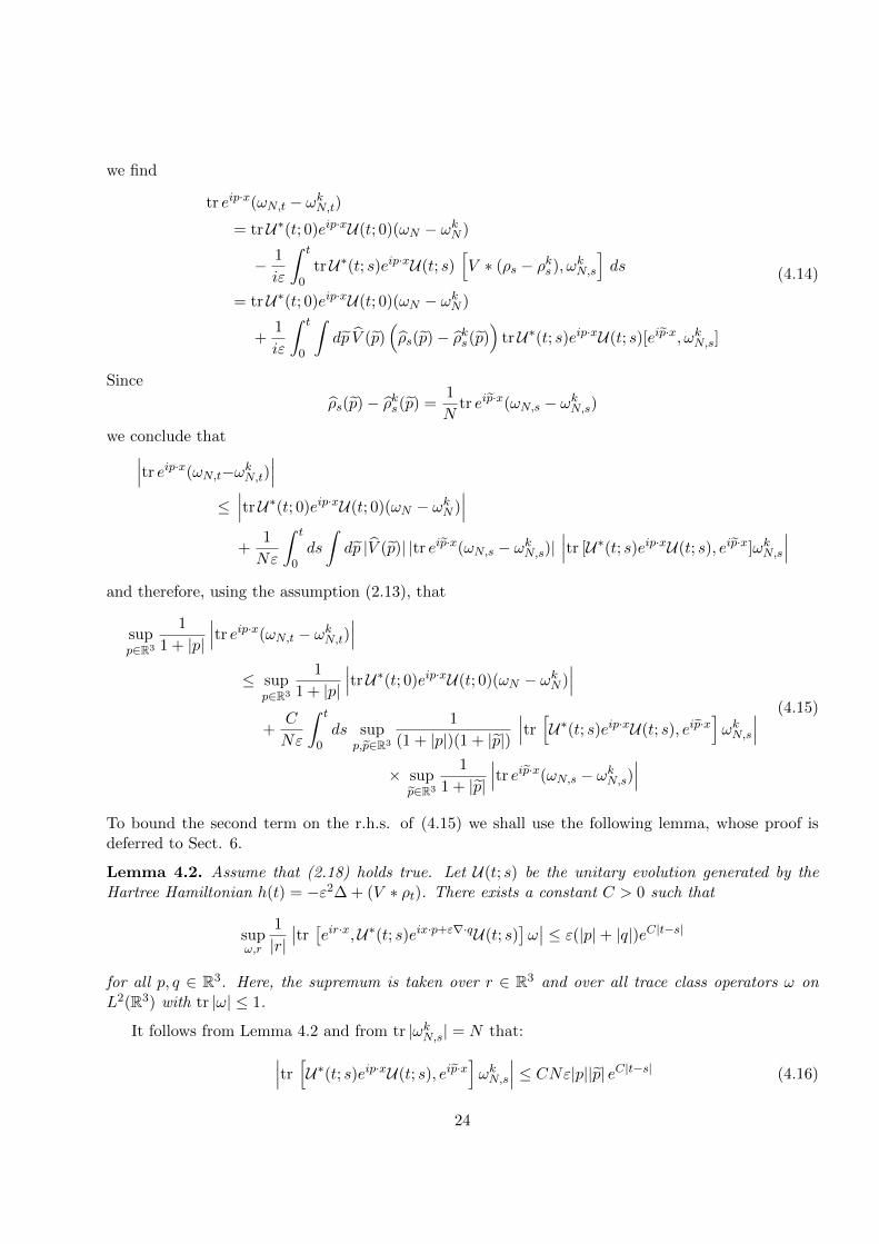
we conclude that∣∣∣tr eip·x(ωN,t−ωkN,t)∣∣∣

≤∣∣∣trU∗(t; 0)eip·xU(t; 0)(ωN − ωkN )

∣∣∣+

1

Nε

∫ t

0ds

∫dp |V (p)| |tr eip·x(ωN,s − ωkN,s)|

∣∣∣tr [U∗(t; s)eip·xU(t; s), eip·x]ωkN,s

∣∣∣and therefore, using the assumption (2.13), that

supp∈R3

1

1 + |p|

∣∣∣tr eip·x(ωN,t − ωkN,t)∣∣∣

≤ supp∈R3

1

1 + |p|

∣∣∣trU∗(t; 0)eip·xU(t; 0)(ωN − ωkN )∣∣∣

+C

Nε

∫ t

0ds sup

p,p∈R3

1

(1 + |p|)(1 + |p|)

∣∣∣tr [U∗(t; s)eip·xU(t; s), eip·x]ωkN,s

∣∣∣× sup

p∈R3

1

1 + |p|

∣∣∣tr eip·x(ωN,s − ωkN,s)∣∣∣

(4.15)

To bound the second term on the r.h.s. of (4.15) we shall use the following lemma, whose proof isdeferred to Sect. 6.

Lemma 4.2. Assume that (2.18) holds true. Let U(t; s) be the unitary evolution generated by theHartree Hamiltonian h(t) = −ε2∆ + (V ∗ ρt). There exists a constant C > 0 such that

supω,r

1

|r|∣∣tr [eir·x,U∗(t; s)eix·p+ε∇·qU(t; s)

]ω∣∣ ≤ ε(|p|+ |q|)eC|t−s|

for all p, q ∈ R3. Here, the supremum is taken over r ∈ R3 and over all trace class operators ω onL2(R3) with tr |ω| ≤ 1.

It follows from Lemma 4.2 and from tr |ωkN,s| = N that:∣∣∣tr [U∗(t; s)eip·xU(t; s), eip·x]ωkN,s

∣∣∣ ≤ CNε|p||p| eC|t−s| (4.16)

24

To bound the first term on the r.h.s. of (4.15), we proceed as follows. We choose a function χ< ∈C∞(R3), with χ<(x) = 1 for |x| ≤ 1 and χ<(x) = 0 for |x| ≥ 2. We set χ> = 1−χ<. For an arbitraryR ≥ 1, we decompose

trU∗(t; 0)eip·xU(t; 0)(ωN − ωkN )

= trU∗(t; 0)eip·xU(t; 0)χ<(−ε2∆/R)(ωN − ωkN )

+ trU∗(t; 0)eip·xU(t; 0)χ>(−ε2∆/R)(ωN − ωkN )χ<(−ε2∆/R)

+ trU∗(t; 0)eip·xU(t; 0)χ>(−ε2∆/R)(ωN − ωkN )χ>(−ε2∆/R)

= I + II + III

(4.17)

To estimate the last term, we observe that

|III| ≤ trχ2>(−ε2∆/R)ωN + trχ2

>(−ε2∆/R)ωkN

≤ 1

R

[tr (−ε2∆)ωN + tr (−ε2∆)ωkN

]=N

R

[∫dxdv v2WN (x, v) +

∫dxdv v2W k

N (x, v)

]≤ CN

R

(4.18)

from the assumption supN ‖WN‖H24< ∞, and using that χ>(−ε2∆/R) ≤ (−ε2∆/R). Next, let us

consider the first term on the r.h.s. of (4.17). We write

I = trU∗(t; 0)eip·xU(t; 0)χ<(−ε2∆/R)(1 + x2)−1(1 + x2)(ωN − ωkN )

and we decompose

[(1 + x2)(ωN − ωkN )

](x; y) = N(1 + x2)

∫dv

[WN

(x+ y

2, v)−W k

N

(x+ y

2, v)]eiv·

(x−y)ε

= D1(x; y) +D2(x; y) +D3(x; y)

where

D1(x; y) = N

[1 +

(x+ y

2

)2]∫

dv

[WN

(x+ y

2, v)−W k

N

(x+ y

2, v)]eiv·

(x−y)ε

is the Weyl quantization of the function (1 + x2)(WN (x, v)−W kN (x, v)) defined on phase-space, while

D2(x; y) =Nε2

4

(x− yε

)2 ∫dv

[WN

(x+ y

2, v)−W k

N

(x+ y

2, v)]eiv·

(x−y)ε

=Nε2

4

∫dv

[∆vWN

(x+ y

2, v)−∆vW

kN

(x+ y

2, v)]eiv·

(x−y)ε

is the Weyl quantization of (ε2/4)(∆vWN (x, v)−∆vWkN (x, v)) and

D3(x; y) = Nεx+ y

2· x− y

ε

∫dv

[WN

(x+ y

2, v)−W k

N

(x+ y

2, v)]eiv·

(x−y)ε

= Nεx+ y

2·∫dv

[∇vWN

(x+ y

2, v)−∇vW k

N

(x+ y

2, v)]eiv·

(x−y)ε

25

is the Weyl quantization of εx · (∇vWN (x, v)−∇vW kN (x, v)). We bound the contributions of the three

terms D1, D2, D3 separately. We begin with∣∣∣trU∗(t; 0)eip·xU(t; 0)χ<(−ε2∆/R)(1 + x2)−1D1

∣∣∣=∣∣∣trU∗(t; 0)eip·xU(t; 0)χ<(−ε2∆/R)(1 + x2)−1(1− ε2∆)−1(1− ε2∆)D1

∣∣∣≤ ‖(1 + x2)−1(1− ε2∆)−1‖HS‖(1− ε2∆)D1‖HS

≤ C√N‖(1− ε2∆)D1‖HS

where we used that 0 ≤ χ<(−ε2∆/R) ≤ 1. We have[(1− ε2∆)D1

](x; y)

= N(1− ε2∆x)

[1 +

(x+ y

2

)2]∫

dv

[W0

(x+ y

2, v)−W k

0

(x+ y

2, v)]eiv·

(x−y)ε

It is not difficult to see that:

‖(1− ε2∆)D1‖HS ≤ C√N‖(1 + x2)(1 + v2)(WN −W k

N )‖2+ C√Nε‖WN −W k

N‖H11

+ C√Nε2‖WN −W k

N‖H22

≤ C√N

(1√k

+ ε

)Therefore ∣∣∣trU∗(t; 0)eip·xU(t; 0)χ<(−ε2∆/R)(1 + x2)−1D1

∣∣∣ ≤ CN ( 1√k

+ ε

)(4.19)

The contribution of D2, on the other hand, can be controlled by∣∣∣trU∗(t; 0)eip·xU(t; 0)χ<(−ε2∆/R)(1 + x2)−1D2

∣∣∣≤ ‖χ<(−ε2∆/R)(1 + x2)−1‖HS‖D2‖HS ≤ Cε2

√N‖W0‖H2‖χ<(−ε2∆/R)(1 + x2)−1‖HS

where

‖χ<(−ε2∆/R)(1 + x2)−1‖2HS

= tr (1 + x2)−1(1− ε2∆)−1χ2<(−ε2∆/R)(1− ε2∆)−1(1 + x2)−1

= tr (1 + x2)−1(1− ε2∆)−1(1− ε2∆)2χ2<(−ε2∆/R)(1− ε2∆)−1(1 + x2)−1

≤ CR2‖(1 + x2)−1(1− ε2∆)−1‖2HS

≤ CR2N

Hence, we conclude that∣∣∣trU∗(t; 0)eip·xU(t; 0)χ<(−ε2∆/R)(1 + x2)−1D2

∣∣∣ ≤ CNRε2 (4.20)

We proceed similarly to bound the contribution of the term D3. We find∣∣∣trU∗(t; 0)eip·xU(t; 0)χ<(−ε2∆/R)(1 + x2)−1D3

∣∣∣ ≤ ‖χ<(−ε2∆/R)(1 + x2)−1‖HS‖D3‖HS

≤ CNRε‖WN −W kN‖H1

1

≤ CNRε√k

26

where in the last step we used (4.2). The last equation, combined with (4.19), (4.20) implies that

|I| ≤ CN(

1√k

+ ε+Rε2 +Rε√k

)Analogously, one can show that the same estimate holds for the term II on the r.h.s. of (4.17) as well(in this case, we introduce the identity (1 + x2)(1 + x2)−1 on the right of the difference ωN − ωkN andwe use the cyclicity of the trace). With (4.18), we conclude that∣∣∣trU∗(t; 0)eip·xU(t; 0)(ωN − ωkN )

∣∣∣ ≤ CN ( 1√k

+ ε+Rε2 +Rε√k

+1

R

)Choosing R = ε−1, we obtain∣∣∣trU∗(t; 0)eip·xU(t; 0)(ωN − ωkN )

∣∣∣ ≤ CN ( 1√k

+ ε

)Inserting this bound and (4.16) in (4.15) and applying Gronwall’s lemma, we obtain

supp∈R3

1

1 + |p|

∣∣∣tr eip·x(ωN,t − ωkN,t)∣∣∣ ≤ CeC|t|N ( 1√

k+ ε

)(4.21)

which concludes the proof of (4.13).

Comparison of ωkN,t with ωN,t. We now compare the Vlasov evolution of the regularized initialdata with the Vlasov evolution of the original data. We claim that there exists a constant C > 0,depending on supN ‖WN‖H2

4but not on the higher Sobolev norms, such that:

‖ωN,t − ωkN,t‖HS = N1/2∥∥WN,t − W k

N,t

∥∥2≤ N1/2Ce

C|t|√k

(4.22)

To prove this, let

ρt(x) =

∫dv WN,t(x, v) and ρkt (x) =

∫dv W k

N,t(x, v) (4.23)

be the densities associated with WN,t and W kN,t. For t ∈ R, we denote by (Xt(x, v), Vt(x, v)) and by

(Xkt (x, v), V k

t (x, v)) the flows satisfying the differential equations{Xt(x, v) = 2Vt(x, v)

Vt(x, v) = −∇(V ∗ ρt)(Xt(x, v))(4.24)

and {Xkt (x, v) = 2V k

t (x, v)

V kt (x, v) = −∇(V ∗ ρkt )(Xk

t (x, v))(4.25)

with initial data given by, respectively, X0(x, v) = Xk0 (x, v) = x, V0(x, v) = V k

0 (x, v) = v. We comparethe two flows (Xt, Vt) and (Xk

t , Vkt ). We have

d

dt(Xt −Xk

t )(x, v) = 2(Vt − V kt )(x, v)

d

dt(Vt − V k

t )(x, v) = −∇(V ∗ ρt)(Xt(x, v)) +∇(V ∗ ρkt )(Xkt (x, v))

27

and therefore ∣∣∣∣ ddt(Xt −Xkt )(x, v)

∣∣∣∣ ≤ 2∣∣∣Vt(x, v)− V k

t (x, v)∣∣∣∣∣∣∣ ddt(Vt − V k

t )(x, v)

∣∣∣∣ ≤ C‖ρt − ρkt ‖1 + C∣∣∣Xt(x, v)−Xk

t (x, v)∣∣∣

where we used the assumption (2.13). Gronwall’s lemma implies that∣∣∣Xt(x, v)−Xkt (x, v)

∣∣∣+∣∣∣Vt(x, v)− V k

t (x, v)∣∣∣ ≤ CeC|t| ∫ t

0ds ‖ρs − ρks‖1

≤ CeC|t|∫ t

0ds ‖Ws −W k

s ‖1(4.26)

We will also need to control the difference between derivatives of the flows (Xt(x, v), Vt(x, v)) and(Xk

t (x, v), V kt (x, v)). Integrating the flow equations (4.24), (4.25), we have

∇xXt(x, v) = 1 + 2

∫ t

0∇xVs(x, v)ds

∇xVt(x, v) = −∫ t

0∇2(V ∗ ρs)(Xs(x, v)) · ∇xXs(x, v) ds

(4.27)

which implies that

|∇xXt(x, v)| ≤ 1 + 2

∫ t

0ds |∇xVs(x, v)|

|∇xVt(x, v)| ≤ C∫ t

0ds |∇xXs(x, v)|

and hence, by Gronwall’s lemma, that

|∇xXt(x, v)|+ |∇xVt(x, v)| ≤ eC|t| (4.28)

Analogously, we also find|∇vXt(x, v)|+ |∇vVt(x, v)| ≤ eC|t| (4.29)

and

|∇xXkt (x, v)|+ |∇xV k

t (x, v)| ≤ eC|t|

|∇vXkt (x, v)|+ |∇xV k

t (x, v)| ≤ eC|t|

Moreover, from (4.27), we obtain∣∣∣∇xXt(x, v)−∇xXkt (x, v)

∣∣∣ ≤ 2

∫ t

0ds∣∣∣∇xVs(x, v)−∇xV k

s (x, v)∣∣∣

and thus∣∣∣∇xVt(x, v)−∇xV kt (x, v)

∣∣∣≤∫ t

0ds∣∣∣∇2(V ∗ ρs)(Xs(x, v)) · ∇xXs(x, v)−∇2(V ∗ ρks)(Xk

s (x, v)) · ∇xXks (x, v)

∣∣∣≤ C

∫ t

0ds ‖ρs − ρks‖1 + C

∫ t

0ds |Xs(x, v)−Xk

s (x, v)||∇xXs(x, v)|

+ C

∫ t

0ds |∇xXs(x, v)−∇xXk

s (x, v)|

28

To get the second inequality, we used that

‖∇3V ∗ ρs‖∞ ≤ ‖∇2V ‖∞‖∇WN‖1 ≤ CeC|s|‖WN‖H14

(4.30)

Using (4.28) and (4.26), and applying Gronwall’s lemma, we conclude that∣∣∣∇xXt(x, v)−∇xXkt (x, v)

∣∣∣+ ∣∣∣∇xVt(x, v)−∇xV kt (x, v)

∣∣∣≤ CeC|t|

∫ t

0ds ‖ρs − ρks‖1 + CeC|t|

∫ t

0ds

∫ s

0dr ‖ρr − ρkr‖1

(4.31)

Similarly, we can also show that∣∣∣∇vXt(x, v)−∇vXkt (x, v)

∣∣∣+ ∣∣∣∇vVt(x, v)−∇vV kt (x, v)

∣∣∣≤ CeC|t|

∫ t

0ds ‖ρs − ρks‖1 + CeC|t|

∫ t

0ds

∫ s

0dr ‖ρr − ρkr‖1

(4.32)

Next, we control the L1 norm of the difference WN,t − W kN,t. To this end, we write

‖WN,t − W kN,t‖1 =

∫dxdv

∣∣WN,t(x, v)− W kN,t(x, v)

∣∣=

∫dxdv

∣∣WN (X−t(x, v), V−t(x, v))−W kN (Xk

−t(x, v), V k−t(x, v))

∣∣≤∫dxdv

∣∣WN (X−t(x, v), V−t(x, v))−W kN (X−t(x, v), V−t(x, v))

∣∣+

∫dxdv

∣∣W kN (X−t(x, v), V−t(x, v))−W k

N (Xk−t(x, v), V k

−t(x, v))∣∣

Using that the Vlasov dynamics preserves the volume in phase-space, we get:

‖WN,t − W kN,t‖1 ≤ ‖WN −W k

N‖1

+

∫dxdv

∣∣∣∣∫ 1

0dλ

d

dλW kN

(λ(X−t(x, v), V−t(x, v)) + (1− λ)(Xk

−t(x, v), V k−t(x, v))

)∣∣∣∣≤ ‖WN −W k

N‖1 +

∫dλdxdv

[∣∣(∇xW kN ) (x(x, v, λ), v(x, v, λ))

∣∣∣∣X−t(x, v)−Xk−t(x, v)

∣∣+∣∣(∇vW k

N ) (x(x, v, λ), v(x, v, λ))∣∣∣∣V−t(x, v)− V k

−t(x, v)∣∣]

where we introduced the notation

x(x, v, λ) := λX−t(x, v) + (1− λ)Xk−t(x, v) , v(x, v, λ) := λV−t(x, v) + (1− λ)V k

−t(x, v)

From (4.26), we obtain

‖WN,t−W kN,t‖1 ≤ ‖WN −W k

N‖1 + C

∫ t

0ds eC|s|‖WN,s − W k

N,s‖1

×[ ∫

dλdxdv∣∣(∇xW k

N ) (x(x, v, λ), v(x, v, λ))∣∣+∣∣(∇vW k

N ) (x(x, v, λ), v(x, v, λ))∣∣] (4.33)

29

We observe that∫dxdv

∣∣(∇xW kN ) (x(x, v, λ), v(x, v, λ))

∣∣ =

∫ ∣∣(∇xW kN )(x, v)

∣∣ 1

|J(x, v)|dxdv (4.34)

with the Jacobian

J = det

[λ

(∇xX−t ∇xV−t∇vX−t ∇vV−t

)+ (1− λ)

(∇xXk

−t ∇xV k−t

∇vXk−t ∇vV k

−t

)]To estimate the determinant J(x, v) in (4.34), we proceed as follows. For a fixed constant C > 0

(that later will be chosen large enough), let us define t∗ > 0 such that:

C3 e2Ct∗

√k

= 1/2 (4.35)

We claim that, for all |t| < t∗,

‖WN,t − W kN,t‖1 ≤ C

eC|t|√k

(4.36)

We prove (4.36) for t > 0 (the case of t < 0 can be handled similarly, of course). We set

t0 = inf{t > 0 : ‖WN,t − W k

N,t‖1 >CeC|t|√

k

}(4.37)

and we proceed by contradiction, assuming that t0 < t∗. At time t = 0, we have:

‖WN −W kN‖1 ≤

∫dxdvdx′dv′gk(x− x′, v − v′)|WN (x, v)−WN (x′, v′)|

=1

(2π)3

∫dxdvdrds e−(r2+s2)/2

∣∣∣∣WN

(x+

r√k, v +

s√k

)−WN (x, v)

∣∣∣∣≤ 1

(2π)3

∫dxdvdrds

∫ 1

0dλ e−(r2+s2)/2

×[|r|√k

∣∣∣∣∇xWN

(x+ λ

r√k, v + λ

s√k

)∣∣∣∣+|s|√k

∣∣∣∣∇vWN

(x+ λ

r√k, v + λ

s√k

)∣∣∣∣]≤ 8π

(2π)3

1√k

(‖∇xWN‖1 + ‖∇vWN‖1) ≤ C√k‖WN‖H1

4≤ C√

k(4.38)

where in the last line we estimated the L1-norms by proceeding as in (4.30). Since, moreover, t→ WN,t

and t→ W kN,t are continuous in the L1-topology, by choosing C = 2C in Eq. (4.37), we conclude that

t0 > 0. The continuity property is a standard fact (see e.g. [8]).By definition, for 0 ≤ t ≤ t0, we have (4.36) and therefore, from (4.31) and (4.32),

∣∣∇xX−t(x, v)−∇xXk−t(x, v)

∣∣+∣∣∇xV−t(x, v)−∇xV k

−t(x, v)∣∣ ≤ C2 e

2C|t|√k

and ∣∣∇vX−t(x, v)−∇vXk−t(x, v)

∣∣+∣∣∇vV−t(x, v)−∇vV k

−t(x, v)∣∣ ≤ C2 e

2C|t|√k

30

Writing

J(x, v) = det

[λ

(∇xX−t ∇xV−t∇vX−t ∇vV−t

)+ (1− λ)

(∇xXk

−t −∇xXt ∇xV k−t −∇xV−t

∇vXk−t −∇vX−t ∇vV k

−t −∇vV−t

)]and using that ∣∣∣∣det

(∇xX−t ∇xV−t∇vX−t ∇vV−t

)∣∣∣∣ = 1

we conclude that

||J(x, v)| − 1| ≤ C3 e3C|t|√k

if the constant C > 0 is large enough. From (4.35), and from the assumption t0 < t∗, we concludethat

|J(x, v)| > 1/2

for all 0 ≤ t ≤ t0. Eq. (4.34) implies:∫dxdv

∣∣(∇xW kN ) (x(x, v, λ), v(x, v, λ))

∣∣ ≤ 2

∫dxdv

∣∣∇xW kN (x, v)

∣∣ ≤ C‖W kN‖H1

4≤ C‖WN‖H1

4

for all 0 < t ≤ t0. Similarly, we obtain∫dxdv

∣∣(∇vW kN ) (x(x, v, λ), v(x, v, λ))

∣∣ ≤ C‖WN‖H14

Plugging the last two bounds in the r.h.s. of (4.33), we find that

‖WN,t − W kN,t‖1 ≤ ‖WN −W k

N‖1 + C

∫ t

0ds eC|s|‖WN,s − W k

N,s‖1

for all 0 ≤ t ≤ t0. Eq. (4.38) and Gronwall’s lemma imply that, if the constant C > 0 is sufficientlylarge,

‖WN,t − W kN,t‖1 ≤ C

eC|t|√k

for all 0 ≤ t ≤ t0, in contradiction with the definition of t0. This shows that t0 > t∗. Repeating thesame argument for t < 0, we obtain that

‖WN,t − W kN,t‖1 ≤ C

eC|t|√k

(4.39)

for all |t| < t∗. From (4.26), we also find that

|Xt(x, v)−Xkt (x, v)|+ |Vt(x, v)− V k

t (x, v)| ≤ C2 e2C|t|√k

(4.40)

for all |t| < t∗. Moreover, Eqs. (4.31) and (4.32) imply that

|J(x, v)| ≥ 1/2 (4.41)

for all |t| < t∗ and for all x, v ∈ R3.

31

Finally, we control the difference WN,t − W kN,t in the L2-norm. To this end, we observe that

‖WN,t − W kN,t‖22 =

∫dxdv

∣∣WN (X−t(x, v), V−t(x, v))−W kN (Xk

−t(x, v), V k−t(x, v))

∣∣2≤ 2

∫dxdv

∣∣WN (X−t(x, v), V−t(x, v))−W kN (X−t(x, v)V−t(x, v))

∣∣2+ 2

∫dxdv

∣∣W kN (X−t(x, v), V−t(x, v))−W k

N (Xk−t(x, v), V k

−t(x, v))∣∣2

Using that the Vlasov dynamics preserves the phase-space volume, we get, for all |t| < t∗:

‖WN,t − W kN,t‖22 ≤ 2‖WN −W k

N‖22

+ 2

∫ 1

0dλ

∫dxdv

{∣∣(∇xW kN ) (x(x, v, λ), v(x, v, λ))

∣∣2∣∣X−t(x, v)−Xk−t(x, v)

∣∣2+∣∣(∇vW k

N ) (x(x, v, λ), v(x, v, λ))∣∣2∣∣V−t(x, v)− V k

−t(x, v)∣∣2}

≤ 2‖WN −W kN‖22

+ 2C4e4C|t|

k

∫ 1

0dλ

∫dxdv

[∣∣(∇xW kN )(x, v)

∣∣2 +∣∣(∇vW k

N )(x, v)∣∣2] 1

|J(x, v)|

≤ 10C4e4C|t|

k‖WN‖2H1

To get the first inequality we used the estimate (4.40), while to get the last one we used (4.41). Bydefinition of t∗, we conclude that, after an appropriate change of the constant C > 0,

‖WN,t − W kN,t‖2 ≤

CeC|t|√k

for all t ∈ R (recall that the bounds ‖WN,t‖2, ‖W kN,t‖2 ≤ C are trivial, since the Vlasov equation

preserves the Lp norms). This concludes the proof of (4.22).

Proof of Theorem 2.2. We have, using (4.5), (4.10), (4.22):

‖ωN,t − ωN,t‖HS ≤ ‖ωN,t − ωkN,t‖HS + ‖ωkN,t − ωkN,t‖HS + ‖ωkN,t − ωN,t‖HS

≤ CN1/2

(ε+

1√k

)exp(C exp(C|t|))

1 +3∑j=1

(ε√k)j

(4.42)

for a constant C > 0 that depends on supN ‖WN‖H24

but not on the higher Sobolev norms. Choosing

k = ε−2, we conclude that

‖ωN,t − ωN,t‖HS ≤ CN1/2ε exp(C exp(C|t|))

as claimed. This concludes the proof of Theorem 2.2.

Proof of Theorem 2.3. Let WN,t be the solution of the Vlasov equation with initial data WN . Weestimate

‖WN,t −Wt‖2 ≤ ‖WN,t − WN,t‖2 + ‖WN,t −Wt‖2 (4.43)

32

The first term can be bounded by Theorem 2.2. In particular, (2.15) implies that

‖WN,t − WN,t‖2 ≤ Cε exp(C exp(C|t|)) (4.44)

As for the second term on the r.h.s. of (4.43), we have to compare two solutions of the Vlasovequation, with slightly different initial data. But this is exactly what we did in Step 3 of the proof ofTheorem 2.2. The only ingredients that we used there were a bound for the L1 and for L2 norm of thedifference of the initial data. Now, by assumption we have ‖W0 −WN‖1 ≤ κN,1, ‖W0 −WN‖2 ≤ κN,2and ‖W0‖H2

4≤ C. Therefore, the arguments used in Step 3 of Section 4 imply that

‖WN,t −Wt‖2 ≤ C(κN,1 + κN,2)eC|t|

Together with (4.44), we conclude that

‖WN,t −Wt‖2 ≤ Cε exp(C exp(C|t|)) + C(κN,1 + κN,2) exp(C|t|) .

5 Convergence for the expectation of semiclassical observables

Here we prove Theorem 2.4 and Theorem 2.5. To show Theorem 2.4, we make first the additionalassumption that the Wigner transforms WN of the fermionic operators ωN are so that supN ‖WN‖H4

4<

∞; later, we will relax this assumption with an approximation argument.

Case supN ‖WN‖H44<∞. We use the expression (3.4) for the difference ωN,t − ωN,t to write

tr eip·x+q·ε∇ (ωN,t − ωN,t) =1

ε

∫ t

0tr eip·x+q·ε∇ U(t; s)[V ∗ (ρs − ρs), ωN,s]U∗(t; s)ds

+1

ε

∫ t

0tr eip·x+q·ε∇ U(t; s)Bs U∗(t; s)ds

(5.1)

with Bs as defined in (3.3). We start by considering the first term on the r.h.s. of (5.1). We have

tr eip·x+q·ε∇ U(t; s)[V ∗ (ρs − ρs), ωN,s]U∗(t; s)

=

∫dz (ρs(z)− ρs(z))tr eip·x+q·ε∇ U(t; s)[V (x− z), ωN,s]U∗(t; s)

=

∫dk V (k)

∫dz e−ik·z(ρs(z)− ρs(z))tr eip·x+q·ε∇ U(t; s)[eik·x, ωN,s]U∗(t; s)

=1

N

∫dk V (k) tr e−ik·z(ωN,s − ωN,s) tr eip·x+q·ε∇ U(t; s)[eik·x, ωN,s]U∗(t; s)

(5.2)

Hence∣∣∣tr eip·x+q·ε∇ U(t; s)[V ∗ (ρs − ρs), ωN,s]U(t; s)ds∣∣∣

≤ 1

N

∫dk |V (k)|

∣∣∣tr eik·x(ωN,s − ωN,s)∣∣∣ ∣∣∣tr eip·x+q·ε∇ U(t; s)[eik·x, ωN,s]U∗(t; s)

∣∣∣≤C tr |ωN,s|

Nsupk∈R3

1

(1 + |k|)2

∣∣∣tr eik·x(ωN,s − ωN,s)∣∣∣

× supω,k

1

|k|

∣∣∣tr [eik·x,U∗(t; s)eip·x+q·ε∇ U(t; s)]ω∣∣∣

(5.3)

33

where we used the assumption (2.18) and where the supremum is taken over all k ∈ R3 and all ω withtr |ω| ≤ 1. From Lemma 4.2, we obtain∣∣∣tr eip·x+q·ε∇U(t; s)[V ∗ (ρs − ρs), ωN,s]U(t; s)ds

∣∣∣≤C tr |ωN,s|

Nε(|p|+ |q|)eC|t−s| sup

k

1

(1 + |k|)2

∣∣∣tr eik·x(ωN,s − ωN,s)∣∣∣ (5.4)

Consider now the second term on the r.h.s. of (5.1). By the cyclicity of the trace, we find

tr eip·x+q·ε∇ U(t; s)Bs U∗(t; s) = trU∗(t; s) eip·x+q·ε∇ U(t; s)Bs . (5.5)

We recall that the kernel of the operator Bs is

Bs(x; y) =

[(V ∗ ρs)(x)− (V ∗ ρs)(y)−∇(V ∗ ρs)

(x+ y

2

)· (x− y)

]ωN,s(x; y) ,

Expanding the parenthesis with the potentials in Fourier integrals, we obtain[(V ∗ρs)(x)−(V ∗ρs)(y)−∇(V ∗ρs)

(x+ y

2

)·(x−y)

]=

∫dk U(k)

(eik·x − eik·y − eik·

(x+y)2 ik · (x− y)

)with U = V ∗ ρs. We write

eik·x − eik·y =

∫ 1

0dλ

d

dλeik·(λx+(1−λ)y) =

∫ 1

0dλeik·(λx+(1−λ)y)ik · (x− y)

and hence

eik·x − eik·y − eik·x+y2 ik · (x− y) =

∫ 1

0dλ[eik·(λx+(1−λ)y) − eik·

x+y2

]ik · (x− y)

=

∫ 1

0dλ

∫ 1

0dµ eik·[µ(λx+(1−λ)y)+(1−µ)(x+y)/2](λ− 1/2)[k · (x− y)]2

This implies that

Bs =3∑

i,j=1

∫ 1

0dλ (λ− 1/2)

∫ 1

0dµ

∫dk U(k)kikj

[xi,[xj , e

i(µλ+(1−µ)/2)k·xωN,sei(µ(1−λ)+(1−µ)/2)k·x

]]Therefore, we can bound the absolute value of the second term on the r.h.s. of (5.1) by∣∣∣tr eip·x+q·ε∇ U(t; s)Bs U∗(t; s)

∣∣∣≤

3∑i,j=1

∫ 1

0dλ|λ− 1/2|

∫ 1

0dµ

∫dk|U(k)||k|2

×∣∣∣trU∗(t; s)eip·x+q·ε∇U(t; s)[xi, [xj , e

i(µλ+(1−µ)/2)k·xωN,sei(µ(1−λ)+(1−µ)/2)k·x]]

∣∣∣=

3∑i,j=1

∫ 1

0dλ|λ− 1/2|

∫ 1

0dµ

∫dk|U(k)||k|2

×∣∣∣tr [xi, [xj ,U∗(t; s)eip·x+q·ε∇U(t; s)]] ei(µλ+(1−µ)/2)k·xωN,se

i(µ(1−λ)+(1−µ)/2)k·x∣∣∣

≤ Ctr|ωN,s|∫dk |U(k)||k|2 sup

ω,i,j

∣∣tr [xi, [xj ,U∗(t; s)eip·x+q·ε∇U(t; s)]]ω∣∣ .

(5.6)

34

The supremum on the r.h.s. is taken over all indices i, j ∈ {1, 2, 3} and all trace class operators ωwith tr |ω| ≤ 1. This term is controlled thanks to the next lemma, whose proof is deferred to the endof the section.

Lemma 5.1. Under the same assumptions of Theorem 2.4, there exists C > 0 such that

supi,j,ω

∣∣tr [xi [xj , U∗(t; s) eip·x+q·ε∇ U(t; s) ]]ω∣∣ ≤ Cε2(|p|+ |q|)2eC|t−s| (5.7)

where the supremum is taken over all i, j ∈ {1, 2, 3} and over all trace class operators on L2(R3) withtr |ω| ≤ 1.

Using |U(k)| ≤ |V (k)|, the assumption (2.18) and (5.7), we conclude that∣∣∣tr eip·x+q·ε∇ U(t; s)Bs U∗(t; s)∣∣∣ ≤ Ctr |ωN,s| (|p|+ |q|)2ε2eC|t−s| (5.8)

Inserting (5.4) and (5.8) on the r.h.s. of (5.1), we obtain

supp,q∈R3

1

(|p|+ |q|+ 1)2

∣∣tr eip·x+q·ε∇ (ωN,t − ωN,t)∣∣

≤ C∫ t

0ds

tr |ωN,s|N

eC|t−s| supk

1

(1 + |k|)2

∣∣∣tr eik·x(ωN,s − ωN,s)∣∣∣

+ C

∫ t

0ds tr |ωN,s|εeC|t−s|

≤ C∫ t

0ds

tr |ωN,s|N

eC|t−s| supp,q

1

(1 + |p|+ |q|)2

∣∣tr eip·x+q·ε∇(ωN,s − ωN,s)∣∣

+ C

∫ t

0ds tr |ωN,s| ε eC|t−s|

(5.9)

Now, we estimate the trace norm of ωN,s (here we need the additional regularity of the Wignertransforms of the initial data assumed at the beginning of the proof). We have

tr |ωN,s| = tr∣∣(1− ε2∆)−1(1 + x2)−1(1 + x2)(1− ε2∆)ωN,s

∣∣≤ ‖(1− ε2∆)−1(1 + x2)−1‖HS‖(1 + x2)(1− ε2∆)ωN,s‖HS

≤ C√N‖(1 + x2)(1− ε2∆)ωN,s‖HS

(5.10)

The operator K = (1 + x2)(1− ε2∆) ωN,s has the integral kernel

K(x; y) = N(1 + x2)(1− ε2∆x)

∫dv WN,s

(x+ y

2, v)e−iv·

x−yε

= N(1 + x2)

∫dv WN,s

(x+ y

2, v)e−iv·

x−yε

+N(1 + x2)

∫dv v2WN,s

(x+ y

2, v)e−iv·

x−yε

− ε2N(1 + x2)

∫dv (∆vWN,s)

(x+ y

2, v)e−iv·

x−yε

+ iεN(1 + x2)

∫dv v · ∇vWN,s

(x+ y

2, v)e−iv·

x−yε

35

Writing

(1 + x2) = 1 +

(x+ y

2

)2

+

(x− yε

)2

we conclude that

‖K‖HS ≤ C√N

4∑j=0

εj‖WN,s‖Hj4

The propagation of regularity of the Vlasov equation from Proposition B.1 gives us

‖K‖HS ≤ C√NeC|s|

4∑j=0

εj‖WN‖Hj4

and thus, with (5.10),

tr |ωN,s| ≤ CNeC|s|4∑j=0

εj‖WN‖Hj4

Inserting in (5.9) and applying Gronwall’s inequality, we find

supp,q∈R3

1

(1 + |p|+ |q|)2

∣∣tr eip·x+q·ε∇(ωN,t − ωN,t)∣∣

≤ C[ 4∑j=0

εj‖WN‖Hj4

]Nε exp

(C[ 4∑j=0

εj‖WN‖Hj4

]exp(C|t|)

) (5.11)

This completes the proof of Theorem 2.4, under the additional assumption that ‖WN‖H44

isbounded.

Proof of Theorem 2.4. We have to relax the condition sup ‖WN‖H44<∞. To this end, we proceed

as follows. We set

W kN (x, v) = (WN ∗ gk)(x, v) =

∫dx′dv′gk(x− x′, v − v′)WN (x′, v′)

with

gk(x, v) =k3

(2π)3e−

k2

(x2+v2)

and we denote by ωkN the Weyl quantization of W kN . We recall from (4.3), that

ωkN (x; y) =1

(2π)3

∫dwdz e−z

2/2e−w2/2[eiw· x√

kε ez√k·∇ωNe

− z√k·∇e−iw· x√

kε

](x; y) (5.12)

is a fermionic reduced density with 0 ≤ ωkN ≤ 1 and trωkN = N . In fact, (5.12), together with theassumption (2.19), also implies that

tr∣∣ωN − ωkN ∣∣ ≤ C N√

k(5.13)

To see this, we write:

tr∣∣ωN − ωkN ∣∣ ≤ 1

(2π)3

∫dwdz e−z

2/2e−w2/2 tr

∣∣∣eiw· x√kε e

z√k·∇ωNe

− z√k·∇e−iw· x√

kε − ωN∣∣∣ ,

36

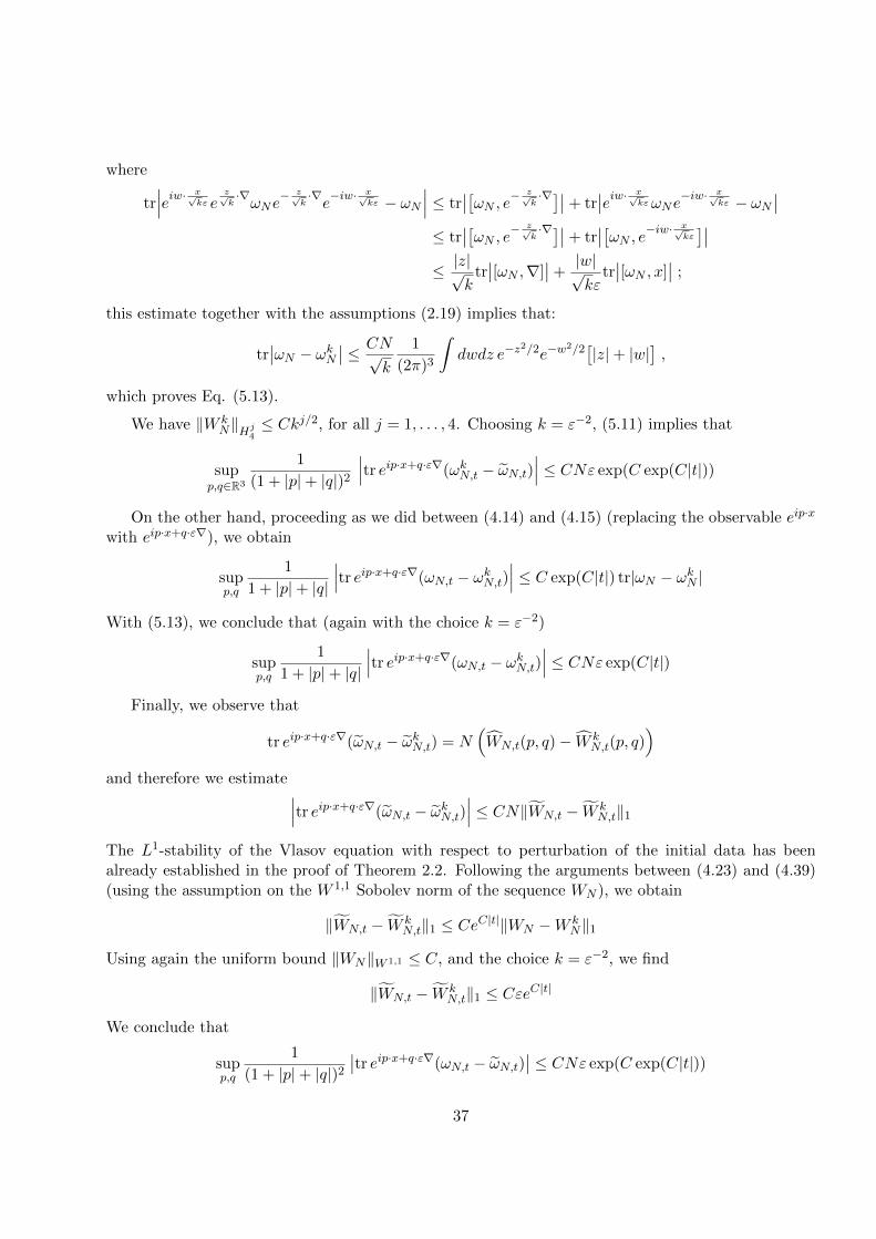
where

tr∣∣∣eiw· x√

kε ez√k·∇ωNe

− z√k·∇e−iw· x√

kε − ωN∣∣∣ ≤ tr

∣∣[ωN , e− z√k·∇]∣∣+ tr

∣∣eiw· x√kεωNe

−iw· x√kε − ωN

∣∣≤ tr

∣∣[ωN , e− z√k·∇]∣∣+ tr

∣∣[ωN , e−iw· x√kε]∣∣

≤ |z|√k

tr∣∣[ωN ,∇]

∣∣+|w|√kε

tr∣∣[ωN , x]

∣∣ ;

this estimate together with the assumptions (2.19) implies that:

tr∣∣ωN − ωkN ∣∣ ≤ CN√

k

1

(2π)3

∫dwdz e−z

2/2e−w2/2[|z|+ |w|

],

which proves Eq. (5.13).

We have ‖W kN‖Hj

4≤ Ckj/2, for all j = 1, . . . , 4. Choosing k = ε−2, (5.11) implies that

supp,q∈R3

1

(1 + |p|+ |q|)2

∣∣∣tr eip·x+q·ε∇(ωkN,t − ωN,t)∣∣∣ ≤ CNε exp(C exp(C|t|))

On the other hand, proceeding as we did between (4.14) and (4.15) (replacing the observable eip·x

with eip·x+q·ε∇), we obtain

supp,q

1

1 + |p|+ |q|

∣∣∣tr eip·x+q·ε∇(ωN,t − ωkN,t)∣∣∣ ≤ C exp(C|t|) tr|ωN − ωkN |

With (5.13), we conclude that (again with the choice k = ε−2)

supp,q

1

1 + |p|+ |q|

∣∣∣tr eip·x+q·ε∇(ωN,t − ωkN,t)∣∣∣ ≤ CNε exp(C|t|)

Finally, we observe that

tr eip·x+q·ε∇(ωN,t − ωkN,t) = N(WN,t(p, q)− W k

N,t(p, q))

and therefore we estimate ∣∣∣tr eip·x+q·ε∇(ωN,t − ωkN,t)∣∣∣ ≤ CN‖WN,t − W k

N,t‖1

The L1-stability of the Vlasov equation with respect to perturbation of the initial data has beenalready established in the proof of Theorem 2.2. Following the arguments between (4.23) and (4.39)(using the assumption on the W 1,1 Sobolev norm of the sequence WN ), we obtain

‖WN,t − W kN,t‖1 ≤ CeC|t|‖WN −W k

N‖1

Using again the uniform bound ‖WN‖W 1,1 ≤ C, and the choice k = ε−2, we find

‖WN,t − W kN,t‖1 ≤ CεeC|t|

We conclude that

supp,q

1

(1 + |p|+ |q|)2

∣∣tr eip·x+q·ε∇(ωN,t − ωN,t)∣∣ ≤ CNε exp(C exp(C|t|))

37

for any sequence of initial densities ωN satisfying (2.19) and whose Wigner transforms WN satisfy‖WN‖W 1,1 ≤ C uniformly in N .

Proof of Theorem 2.5. We write∣∣∣WN,t(p, q)− Wt(p, q)∣∣∣ ≤ ∣∣∣∣WN,t(p, q)−

WN,t(p, q)

∣∣∣∣+

∣∣∣∣WN,t(p, q)− Wt(p, q)

∣∣∣∣where WN,t denotes the solution of the Vlasov equation with initial data WN . From Theorem 2.4, weknow that ∣∣∣∣WN,t(p, q)−

WN,t(p, q)

∣∣∣∣ ≤ Cε(1 + |p|+ |q|)2eC|t|

To conclude the proof of the theorem, we need to compare the solutions WN,t and Wt of the Vlasovequation, using the fact that the two initial data are close in L1. As in the approximation argumentused in the proof of Theorem 2.4, we make use of the L1-stability of the solution of the Vlasov equation,established in Step 3 of the proof of Theorem 2.2. Following the arguments between (4.23) and (4.39),we obtain

‖WN,t −Wt‖1 ≤ CeC|t|‖WN −W0‖1where the constant C > 0 depends only on ‖W0‖W 1,1 . This implies that

‖WN,t − Wt‖∞ ≤ ‖WN,t −Wt‖1 ≤ CκNeC|t|

Hence, ∣∣∣WN,t(p, q)− Wt(p, q)∣∣∣ ≤ C(1 + |p|+ |q|)2(ε+ κN )eC|t|

which concludes the proof Theorem 2.5.

6 Proof of auxiliary lemmas

In this section we show Lemma 4.2 and Lemma 5.1.

Proof of Lemma 4.2. We define the unitary evolution U(t; s) satisfying

iε∂t U(t; s) = eir·x h(t) e−ir·x U(t; s)

= (h(t) + 2iε2r · ∇+ r2ε2) U(t; s)(6.1)

We observe that

supω

∣∣tr [eir·x,U∗(t; s)eix·p+ε∇·qU(t; s)]ω∣∣ = sup

ω

∣∣∣tr [eir·x,U∗(t; s)eix·p+ε∇·qU(t; s)]U(s; 0)ωU∗(s; 0)

∣∣∣= sup

ω

∣∣∣tr U∗(s; 0)[eir·x,U∗(t; s)eix·p+ε∇·qU(t; s)

]U(s; 0)ω

∣∣∣(6.2)

where the supremum is taken over all trace class operators ω on L2(R3) with tr |ω| ≤ 1 and where weused the fact that tr |U(s; 0)ωU∗(s; 0)| ≤ tr |ω|. For a fixed ω and for fixed t ∈ R, we compute now the

38

time-derivative of

iε∂str U∗(s; 0)[eir·x,U∗(t; s)eix·p+ε∇·qU(t; s)

]U(s; 0)ω

= − tr U∗(s; 0) [h(s), [eir·x,U∗(t; s) eix·p+ε∇·q U(t; s)]]U(s; 0)ω

− 2ε2 tr U∗(s; 0) ir · ∇ [eir·x,U∗(t; s) eix·p+ε∇·q U(t; s)]U(s; 0)ω

− ε2 r2 tr U∗(s; 0) [eir·x,U∗(t; s) eix·p+ε∇·q U(t; s)]U(s; 0)ω

+ tr U∗(s; 0) [eir·x, [h(s),U∗(t; s) eix·p+ε∇·q U(t; s)]]U(s; 0)ω

Using the properties of commutators, we find

iε∂str U∗(s; 0)[eir·x,U∗(t; s)eix·p+ε∇·qU(t; s)

]U(s; 0)ω

= − 2ε2 tr U∗(s; 0) ir · ∇ [eir·x,U∗(t; s) eix·p+ε∇·q U(t; s)]U(s; 0)ω

− ε2 r2 tr U∗(s; 0) [eir·x,U∗(t; s) eix·p+ε∇·q U(t; s)]U(s; 0)ω

+ tr U∗(s; 0) [U∗(t; s) eix·p+ε∇·q U(t; s), [h(s), eir·x]]U(s; 0)ω

(6.3)

We have[h(s) , eir·x] = (−2iε2r · ∇ − ε2r2) eir·x .

Inserting this expression in (6.3), we get

iε∂str U∗(s; 0)[eir·x,U∗(t; s)eix·p+ε∇·qU(t; s)

]U(s; 0)ω

= 2εtr U∗(s; 0) [U∗(t; s) eix·p+ε∇·q U(t; s), ir · ε∇] eir·x U(s; 0)ω(6.4)

Integrating this equation from time s to time t, we find

tr U∗(s; 0)[eir·x,U∗(t; s)eix·p+ε∇·qU(t; s)

]U(s; 0)ω

= tr U∗(t; 0)[eir·x, eix·p+ε∇·q

]U(t; 0)ω

+ 2i

∫ t

sdτ tr U∗(τ ; 0) [U∗(t; τ) eix·p+ε∇·q U(t; τ), ir · ε∇] eir·x U(τ ; 0)ω

which implies that∣∣∣tr U∗(s; 0)[eir·x,U∗(t; s)eix·p+ε∇·qU(t; s)

]U(s; 0)ω

∣∣∣≤∣∣∣tr [eir·x, eix·p+ε∇·q]U(t; 0)ωU∗(t; 0)

∣∣∣+ 2

∫ t

sdτ∣∣∣tr [U∗(t; τ)eix·p+ε∇·qU(t; τ), ir · ε∇

]eir·xU(τ ; 0)ω U∗(τ ; 0)

∣∣∣Since

[eir·x, eix·p+ε∇·q] = (e−iεr·q/2 − eiεr·q/2)eix·(p+r)+ε∇·q

we conclude that, for any trace class operator ω on L2(R3), with tr |ω| ≤ 1, we have

1

|r|

∣∣∣tr [eir·x,U∗(t; s)eix·p+ε∇·qU(t; s)]U(s; 0)ω U∗(s; 0)

∣∣∣≤ ε|q|+ 2

∫ t

sdτ sup

ω

∣∣∣∣tr [U∗(t; τ)eix·p+ε∇·qU(t; τ), ir

|r|· ε∇

]ω

∣∣∣∣39

where, on the r.h.s., the supremum is taken over all trace class ω with tr |ω| ≤ 1. From (6.2), weobtain

supω,r

∣∣∣tr [eir·x,U∗(t; s)eix·p+ε∇·qU(t; s)]ω∣∣∣

≤ ε|q|+ 2

∫ t

sdτ sup

ω,r

∣∣∣∣tr [i r|r| · ε∇,U∗(t; τ)eix·p+ε∇·qU(t; τ)

]ω

∣∣∣∣ (6.5)

Next, we bound the supremum on the r.h.s. of the last equation. To this end, we observe that

supω

∣∣∣∣tr [i r|r| · ε∇,U∗(t; s)eix·p+ε∇·qU(t; s)

]ω

∣∣∣∣= sup

ω

∣∣∣∣tr [U∗(t; s)eix·p+ε∇·qU(t; s), ir

|r|· ε∇

]U(s; 0)ωU∗(s; 0)

∣∣∣∣= sup

ω

∣∣∣∣trU∗(s; 0)

[U∗(t; s)eix·p+ε∇·qU(t; s), i

r

|r|· ε∇

]U(s; 0)ω

∣∣∣∣(6.6)

We compute

iε∂strU∗(s; 0)[U∗(t; s)eix·p+ε∇·qU(t; s), ir · ε∇

]U(s; 0)ω

= − trU∗(s; 0) [h(s) , [U∗(t; s) eix·p+ε∇·q U(t; s) , iεr · ∇]]U(s; 0)ω

+ trU∗(s; 0) [[h(s) , U∗(t; s) eix·p+ε∇·q U(t; s)] , iεr · ∇]U(s; 0)ω

The Jacobi identity implies that

iε∂strU∗(s; 0)[U∗(t; s)eix·p+ε∇·qU(t; s), ir · ε∇

]U(s; 0)ω

= − trU∗(s; 0) [U∗(t; s) eix·p+ε∇·q U(t; s) , [h(s) , iεr · ∇]]U(s; 0)ω .(6.7)

We have

[h(s), ir · ε∇] = iεr · ∇(V ∗ ρs)(x) = iεr ·∫dkkV (k)ρs(k)eik·x

Hence

iε∂strU∗(s; 0)[U∗(t; s)eix·p+ε∇·qU(t; s), ir · ε∇

]U(s; 0)ω

= − iε ·∫dkr · kV (k)ρt(k) trU∗(s; 0) [U∗(t; s) eix·p+ε∇·q U(t; s) , eik·x]U(s; 0)ω .

Integrating from time s to time t, we find

trU∗(s; 0)[U∗(t; s)eix·p+ε∇·qU(t; s), ir · ε∇

]U(s; 0)ω

= trU∗(t; 0)[eix·p+ε∇·q, ir · ε∇

]U(t; 0)ω

+ i

∫ t

sdτ

∫dkr · kV (k)ρτ (k) trU∗(τ ; 0) [U∗(t; τ) eix·p+ε∇·q U(t; τ) , eik·x]U(τ ; 0)ω

Since [eix·p+ε∇·q, ir · ε∇

]= εr · peix·p+ε∇·q

40

we conclude that, for any trace class operator ω with tr |ω| ≤ 1,∣∣∣trU∗(s; 0)

[U∗(t; s)eix·p+ε∇·qU(t; s), i

r

|r|· ε∇

]U(s; 0)ω

∣∣∣= ε|p|+

∫ t

sdτ sup

ω,k

1

|k|

∣∣∣trU∗(τ ; 0) [U∗(t; τ) eix·p+ε∇·q U(t; τ) , eik·x]U(τ ; 0)ω∣∣∣ ∫ dk|k|2|V (k)|

From (6.6), we find

supω,r

∣∣∣tr [i r|r| · ε∇,U∗(t; s)eix·p+ε∇·qU(t; s)

]ω∣∣∣

≤ ε|p|+ C

∫ t

sdτ sup

ω,r

1

|r|

∣∣∣trU∗(τ ; 0) [U∗(t; τ) eix·p+ε∇·q U(t; τ) , eik·x]U(τ ; 0)ω∣∣∣

Combining this bound with (6.5) and applying Gronwall, we obtain

supω,r

∣∣∣tr [eir·x,U∗(t; s)eix·p+ε∇·qU(t; s)]ω∣∣∣+ sup

ω,r

∣∣∣tr [i r|r| · ε∇,U∗(t; s)eix·p+ε∇·qU(t; s)

]ω∣∣∣

≤ εN(|p|+ |q|)eC|t−s|

Proof of Lemma 5.1. We observe, first of all, that

supω

∣∣∣tr [xi [xj ,U∗(t; s) eip·x+q·ε∇ U(t; s) ]]ω∣∣∣

= supω

∣∣tr [xi [xj , U∗(t; s) eip·x+q·ε∇ U(t; s) ]]U(s; 0)ωU∗(s; 0)∣∣

= supω

∣∣trU∗(s; 0) [xi [xj , U∗(t; s) eip·x+q·ε∇ U(t; s) ]]U(s; 0)ω∣∣ (6.8)

We consider now the derivative

iε∂strU∗(s; 0) [xi [xj , U∗(t; s) eip·x+q·ε∇ U(t; s) ]]U(s; 0)ω

= − trU∗(s; 0) [h(s), [xi [xj , U∗(t; s) eip·x+q·ε∇ U(t; s) ]]]U(s; 0)ω

+ trU∗(s; 0) [xi [xj , [h(s),U∗(t; s) eip·x+q·ε∇ U(t; s) ]]]U(s; 0)ω

The Jacobi identity implies that

iε∂strU∗(s; 0) [xi [xj , U∗(t; s) eip·x+q·ε∇ U(t; s) ]]U(s; 0)ω

= trU∗(s; 0) [xi [[xj , h(s)],U∗(t; s) eip·x+q·ε∇ U(t; s) ]]U(s; 0)ω

+ trU∗(s; 0) [[xi, h(s)], [xj ,U∗(t; s) eip·x+q·ε∇ U(t; s) ]]U(s; 0)ω

Since [xj , h(s)] = ε2∇xj (and since [∇xj , xi] = δij is a number), we conclude that

iε∂strU∗(s; 0) [xi, [xj , U∗(t; s) eip·x+q·ε∇ U(t; s) ]]U(s; 0)ω

= εtrU∗(s; 0) [ε∇xj , [xi,U∗(t; s) eip·x+q·ε∇ U(t; s) ]]U(s; 0)ω

+ εtrU∗(s; 0) [ε∇xi , [xj ,U∗(t; s) eip·x+q·ε∇ U(t; s) ]]U(s; 0)ω

(6.9)

41

Integrating over time, we find

trU∗(s; 0)[xi, [xj ,U∗(t; s)eip·x+q·ε∇U(t; s)]]U(s; 0)ω

= trU∗(t; 0)[xi, [xj , eip·x+q·ε∇]]U(t; 0)ω

+ i

∫ t

sdτtrU∗(τ ; 0)[ε∇xj , [xi,U∗(t; τ)eip·x+q·ε∇U(t; τ)]]U(τ ; 0)ω

+ i

∫ t

sdτtrU∗(τ ; 0)[ε∇xi , [xj ,U∗(t; τ)eip·x+q·ε∇U(t; τ)]]U(τ ; 0)ω

Since[xi, [xj , e

ip·x+q·ε∇]] = ε2qiqjeip·x+q·ε∇

we find ∣∣trU∗(s; 0)[xi, [xj ,U∗(t; s)eip·x+q·ε∇U(t; s)]]U(s; 0)ω∣∣

≤ ε2|q|2 +

∫ t

sdτ sup

ω,i,j

∣∣tr [ε∇xj , [xi,U∗(t; τ)eip·x+q·ε∇U(t; τ)]]ω∣∣

for all trace class ω with tr |ω| ≤ 1. From (6.8), we obtain

supω,i,j

∣∣tr [xi, [xj ,U∗(t; s)eip·x+q·ε∇U(t; s)]]ω∣∣

≤ ε2|q|2 +

∫ t

sdτ sup

ω,i,j

∣∣tr [ε∇xj , [xi,U∗(t; τ)eip·x+q·ε∇U(t; τ)]]ω∣∣

where the suprema are taken over all trace class ω on L2(R3) with tr |ω| ≤ 1.Next, we look for an estimate for

supω,i,j

∣∣tr [ε∇xj , [xi,U∗(t; s)eip·x+q·ε∇U(t; s)]]ω∣∣

= supω,i,j

∣∣trU∗(s; 0)[ε∇xj , [xi,U∗(t; s)eip·x+q·ε∇U(t; s)]]U(s; 0)ω∣∣

To this end, we compute the derivative

iε∂strU∗(s; 0) [ε∇xi , [xj ,U∗(t; s) eip·x+q·ε∇ U(t; s) ]]U(s; 0)ω

= − trU∗(s; 0) [h(s), [ε∇xi , [xj ,U∗(t; s) eip·x+q·ε∇ U(t; s) ]]]U(s; 0)ω

+ trU∗(s; 0) [ε∇xi , [xj , [h(s),U∗(t; s) eip·x+q·ε∇ U(t; s) ]]]U(s; 0)ω

= trU∗(s; 0) [[ε∇xi , h(s)], [xj ,U∗(t; s) eip·x+q·ε∇ U(t; s) ]]U(s; 0)ω

+ trU∗(s; 0) [ε∇xi , [[xj , h(s)],U∗(t; s) eip·x+q·ε∇ U(t; s) ]]U(s; 0)ω

With

[ε∇xi , h(s)] = ε∇xi(V ∗ ρs)(x) = ε

∫dkkiV (k)ρs(k)eik·x (6.10)

we obtain

iε∂strU∗(s; 0) [ε∇xi , [xj ,U∗(t; s) eip·x+q·ε∇ U(t; s) ]]U(s; 0)ω

= ε

∫dkkiV (k)ρs(k)trU∗(s; 0) [eik·x, [xj ,U∗(t; s) eip·x+q·ε∇ U(t; s) ]]U(s; 0)ω

+ εtrU∗(s; 0) [ε∇xi , [ε∇xi ,U∗(t; s) eip·x+q·ε∇ U(t; s) ]]U(s; 0)ω

42

Using the identity

[eik·x, A] = eik·xA−Aeik·x =

∫ 1

0dλ

d

dλeiλk·xAei(1−λ)k·x =

∫ 1

0dλeiλk·x[ik · x,A]ei(1−λ)k·x (6.11)

we conclude that

iε∂strU∗(s; 0) [ε∇xi , [xj ,U∗(t; s) eip·x+q·ε∇ U(t; s) ]]U(s; 0)ω

= ε

∫ 1

0dλ

∫dkkik`V (k)ρs(k)trU∗(s; 0) eiλk·x[x`, [xj ,U∗(t; s) eip·x+q·ε∇ U(t; s) ]] ei(1−λ)k·xU(s; 0)ω

+ εtrU∗(s; 0) [ε∇xi , [ε∇xi ,U∗(t; s) eip·x+q·ε∇ U(t; s) ]]U(s; 0)ω

and hence, after integrating over time,∣∣∣trU∗(s; 0) [ε∇xi , [xj ,U∗(t; s) eip·x+q·ε∇ U(t; s) ]]U(s; 0)ω∣∣∣

≤∣∣∣trU∗(t; 0) [ε∇xi , [xj , e

ip·x+q·ε∇]]U(t; 0)ω∣∣∣

+

∫ t

sdτ

∫ 1

0dλ

∫dk|k|2|V (k)|

×∣∣∣trU∗(τ ; 0) eiλk·x[x`, [xj ,U∗(t; τ) eip·x+q·ε∇ U(t; τ) ]] ei(1−λ)k·xU(τ ; 0)ω

∣∣∣+

∫ t

sdτ∣∣∣trU∗(τ ; 0) [ε∇xi , [ε∇xj ,U∗(t; τ) eip·x+q·ε∇ U(t; τ) ]]U(τ ; 0)ω

∣∣∣Since

[ε∇xi , [xj , eip·x+qε·∇]] = −iε2piqjeip·x+qε·∇

this implies that

supω,i,j

∣∣∣tr [ε∇xi , [xj ,U∗(t; s) eip·x+q·ε∇ U(t; s) ]]ω∣∣∣

≤ ε2|p||q|+ C

∫ t

sdτ sup

ω,i,j

∣∣tr [xi, [xj ,U∗(t; τ) eip·x+q·ε∇ U(t; τ) ]]ω∣∣

+

∫ t

sdτ sup

ω,i,j

∣∣∣tr [ε∇xi , [ε∇xj ,U∗(t; τ) eip·x+q·ε∇ U(t; τ) ]]ω∣∣∣

(6.12)

Finally, we need an estimate for

supω,i,j

∣∣∣tr [ε∇xi , [ε∇xj ,U∗(t; s) eip·x+q·ε∇ U(t; s) ]]ω∣∣∣

= supω,i,j

∣∣∣trU∗(s, 0)[ε∇xi , [ε∇xj ,U∗(t; s) eip·x+q·ε∇ U(t; s) ]]U(s; 0)ω∣∣∣

Hence, we compute the derivative

iε∂strU∗(s; 0)[ε∇xi , [ε∇xj ,U∗(t; s) eip·x+q·ε∇ U(t; s) ]]U(s; 0)ω

= − trU∗(s; 0)[h(s), [ε∇xi , [ε∇xj ,U∗(t; s) eip·x+q·ε∇ U(t; s) ]]]U(s; 0)ω

+ trU∗(s; 0)[ε∇xi , [ε∇xj , [h(s),U∗(t; s) eip·x+q·ε∇ U(t; s) ]]]U(s; 0)ω

= trU∗(s; 0)[[ε∇xi , h(s)], [ε∇xj ,U∗(t; s) eip·x+q·ε∇ U(t; s)]]U(s; 0)ω

+ trU∗(s; 0)[ε∇xi , [[ε∇xj , h(s)],U∗(t; s) eip·x+q·ε∇ U(t; s)]]U(s; 0)ω

43

From (6.10), we find

iε∂strU∗(s; 0)[ε∇xi , [ε∇xj ,U∗(t; s) eip·x+q·ε∇ U(t; s) ]]U(s; 0)ω

= ε

∫dkkiV (k)ρs(k) trU∗(s; 0)[eik·x, [ε∇xj ,U∗(t; s) eip·x+q·ε∇ U(t; s)]]U(s; 0)ω

+ ε

∫dkkj V (k)ρs(k) trU∗(s; 0)[ε∇xi , [eik·x,U∗(t; s) eip·x+q·ε∇ U(t; s)]]U(s; 0)ω

(6.13)

In the first term on the r.h.s. of the last equation we use (6.11). In the second term, on the otherhand, we notice that

trU∗(s; 0)[ε∇xi ,[eik·x,U∗(t; s) eip·x+q·ε∇ U(t; s)]]U(s; 0)ω

= trU∗(s; 0)[eik·x, [ε∇xi ,U∗(t; s) eip·x+q·ε∇ U(t; s)]]U(s; 0)ω

+ trU∗(s; 0)[[ε∇xi , eik·x],U∗(t; s) eip·x+q·ε∇ U(t; s)]U(s; 0)ω

Again, the first term on the r.h.s. of the last equation can be handled with (6.11). As for the secondterm, we use that [ε∇xi , eik·x] = iεkie

ik·x. Integrating (6.13) over time, we find∣∣∣trU∗(s; 0)[ε∇xi , [ε∇xj ,U∗(t; s) eip·x+q·ε∇ U(t; s) ]]U(s; 0)ω∣∣∣

≤∣∣trU∗(t; 0)[ε∇xi , [ε∇xj , eip·x+q·ε∇ ]]U(t; 0)ω

∣∣+ C

∫ t

sdτ sup

ω,i,j

∣∣tr [ε∇xi , [xj ,U∗(t; τ) eip·x+q·ε∇ U(t; τ)]]ω∣∣

+ Cε

[∫dk |V (k)||ρs(k)||k|3dk

][∫ t

sdτ sup

ω,k

1

|k|

∣∣∣tr [eik·x,U∗(t; τ) eip·x+q·ε∇ U(t; τ)]ω∣∣∣]

To bound the integral involving the potential in the last term on the r.h.s. of the last equation, weuse (2.18) with ‖ρs‖∞ ≤ 1. From

[ε∇xi , [ε∇xj , eip·x+q·ε∇ ] = −ε2pipjeip·x+q·ε∇

and from Lemma 4.2, we obtain∣∣∣trU∗(s; 0)[ε∇xi , [ε∇xj ,U∗(t; s) eip·x+q·ε∇ U(t; s) ]]U(s; 0)ω∣∣∣

≤ Cε2 + C

∫ t

sdτ sup

ω,i,j

∣∣tr [ε∇xi , [xj ,U∗(t; τ) eip·x+q·ε∇ U(t; τ)]]ω∣∣ (6.14)

Combining (6.9) and (6.12) with the last equation and applying Gronwall lemma, we deduce that

supi,j,ω

∣∣∣tr [xi, [xj ,U∗(t; s) eip·x+q·ε∇ U(t; s) ]]ω∣∣∣ ≤ Cε2(|p|+ |q|)2eC|t−s|

supi,j,ω

∣∣∣tr [ε∇xi , [xj ,U∗(t; s) eip·x+q·ε∇ U(t; s) ]]ω∣∣∣ ≤ Cε2(|p|+ |q|)2eC|t−s|

supi,j,ω

∣∣∣tr [ε∇xi , [ε∇xj ,U∗(t; s) eip·x+q·ε∇ U(t; s) ]]ω∣∣∣ ≤ Cε2(|p|+ |q|)2eC|t−s|

44

A Well-posedness of the Vlasov equation for signed measures

The goal of this appendix is to show that the arguments of [8] can be extended to prove the well-posedness of the Vlasov equation (1.10) for initial data given by signed measures.

Following the notation of [8], let M denote the space of all finite signed measures on the Borelσ-algebra B(R6). For an open interval ∆ ⊂ R, we denote by M∆ the set of all families M = {µt}t∈∆,with µt ∈ M for all t ∈ ∆ such that, for all bounded intervals ∆′ ⊂ ∆, there exists C∆′ > 0 withsupt∈∆′ ‖µt‖ < C∆′ , and such that the function

(∇V ∗ µt) (x) =

∫∇V (x− x′) dµt(x′, v′)

is continuous in t ∈ ∆, for all x ∈ R3 (V denotes the interaction potential entering the Vlasovequation (1.10)). For C > 0, we also denote by M∆(κ) the set of families M = {µt}t∈∆ with‖µt‖ = supB∈B(R6) |µ(B)| = κ for all t ∈ ∆.

Defining A,B : R3 × R3 → R3 × R3 by A(x, v) = (2v, 0) and B(x, v) = (0,∇V (x)) and, for everyµ ∈M,

Bµ(x, v) =

∫B(x− x′, v − v′)dµ(x′, v′)

we say that a family M = {µt}t∈∆ ∈M∆ is a weak solution of the Vlasov equation on the interval ∆if, for every test function h ∈ D(R6) in the Schwarz space,

µt(h) =

∫h(x, v)dµt(x, v)

is differentiable in t ∈ ∆ andd

dtµt(h) = µt((A+Bµt)∇h)

It is easy to check that, if the weak solution µt has a density Wt(x, v), differentiable in t, then Wt isa solution of the standard Vlasov equation (1.10).

Proposition A.1. Let V ∈ C2b (R3). For any finite signed measure µ0 ∈ M, and every open interval

∆ ⊂ R with 0 ∈ ∆, there exists a unique weak solution M = {µt}t∈∆ of the Vlasov equation on ∆with µt=0 = µ0.

Proof. We follow the strategy of [8], adapting it to the case of signed µ0. We will use the variablez = (x, v) ∈ R6. For M = {µt}t∈∆ ∈M∆, we define

GM (t, z) = A(z) +Bµt(z) (A.1)

and we consider the solution of Newton’s equation

d

dtz(t) = GM (t, z(t)) (A.2)

We denote by zM (t, u) the solution of (A.2), with initial data zM (0, u) = u.For a fixed µ0 ∈M, we define the map T :M∆ →M∆ by

(TM)t(E) = µ0({u ∈ R6 : zM (t, u) ∈ E

})45

for all E ∈ B(R6). As in [8], it is easy to check that M ∈M∆ is a weak solution of the Vlasov equationwith initial data µ0 if and only if M is a fixed point of T , i.e. if TM = M .

Hence, to prove Proposition A.1, it is enough to show that T is a contraction on M∆. In fact,since clearly TM ∈ M∆(‖µ0‖), for all M ∈ M∆, it is enough to show that the restriction of T toM∆(‖µ0‖) is a contraction, with respect to an appropriate metric, that we are now going to define.

For two signed measures µ, µ′ ∈M, we define

d(µ, µ′) = dKR(µ+, µ′+) + dKR(µ−, µ

′−) (A.3)

where µ = µ+−µ− is the Jordan decomposition of µ in its positive and negative parts and where dKRis the Kantorovich-Rubinshtein metric, defined by

dKR(ν, ν ′) = infm∈N(ν,ν′)

∫ρ(z1, z2)dm(z1, z2)

where ρ(z1, z2) = min(|z1 − z2|, 1) and N(ν, ν ′) is the space of all positive measures m on B(R12)such that m(E × R6) = ν(E) and m(R6 × E) = ν ′(E) for all E ∈ B(R6). Furthermore, for M ={µt}t∈∆,M

′ = {µ′t}t∈∆ ∈M∆, we define

d(M,M ′) =

∫∆d(µt, µ

′t)

It is easy to check that (A.3) defines a metric on M(∆).We claim that, for |∆| small enough,

d(TM, TM ′) ≤ 1

2d(M,M ′) (A.4)

for all M,M ′ ∈M∆(‖µ0‖). To prove (A.4) we observe that, for all µ, µ′ ∈M,

Bµ(z)−Bµ′(z) =

∫B(z − w)dµ(w)−

∫B(z − w)dµ′(w)

≤∫

(B(z − w1)−B(z − w2))dm+(w1, w2)

−∫

(B(z − w1)−B(z − w2))dm−(w1, w2)

for any m+ ∈ N(µ+, µ′+),m− ∈ N(µ−, µ

′−). Recalling that B(x, v) = (0,∇V (x)) and the assumption

V ∈ C2b (R3), we find

|Bµ(z)−Bµ′(z)| ≤∫|B(z − w1)−B(z − w2)|dm+(w1, w2)

+

∫|B(z − w1)−B(z − w2)|dm−(w1, w2)

≤ C∫ρ(w1, w2)dm+(w1, w2) +

∫ρ(w1, w2)dm−(w1, w2)

Since the inequality holds for every m+ ∈ N(µ+, µ′+) and m− ∈ N(µ−, µ

′−), we conclude that

|Bµ(z)−Bµ′(z)| ≤ Cd(µ, µ′) (A.5)

46

for all µ, µ′ ∈M and all z ∈ R6.Furthermore, recalling the definition (A.1), we observe that there is a constant C, depending on

‖µ0‖, such that|GM (z)−GM (z′)| ≤ C|z − z′| (A.6)

for all z, z′ ∈ R6 and for all M ∈M∆(‖µ0‖).For M,M ′ ∈M∆(‖µ0‖) and u ∈ R6, we define the quantity

α(M,M ′, u) = supt∈∆|zM (t, u)− zM ′(t, u)|

With (A.6), we obtain

|zM (t, u)− zM ′(t, u)| ≤∫ t

0|GM (s, zM (s, u)−GM ′(s, zM ′(s, u))|ds

≤∫

∆|GM (s, zM (s, u)−GM (s, zM ′(s, u))|ds

+

∫∆GM (s, zM ′(s, u)−GM ′(s, zM ′(s, u))|ds

for all t ∈ ∆. Combining (A.5) and (A.6), we find

|zM (t, u)− zM ′(t, u)| ≤ C∫

∆|zM (s, u)− zM ′(s, u)|ds+ Cd(M,M ′)

Taking the supremum over t, we conclude that, for sufficiently small |∆|,

α(M,M ′, u) ≤ C

1− C|∆|d(M,M ′)

We are now ready to bound d(TM, TM ′). For M,M ′ ∈M∆(‖µ0‖), we notice that

(TMt)±(E) = µ0±({u ∈ R6 : zM (t, u) ∈ E}

)for every E ∈ B(R6). Now, let

mt,±(F ) = µ0±({u ∈ R6 : (zM (t, u), zM ′(t, u)) ∈ F}

)for every F ∈ B(R12). Then we have mt,± ∈ N((TMt)±, (TM

′t)±) and∫

ρ(z1, z2)dmt,±(z1, z2) =

∫ρ(zM (t, u), zM ′(t, u))dµ0

±(u)

≤∫α(M,M ′, u)dµ0

±(u)

≤C‖µ0

±‖1− C|∆|

d(M,M ′)

This implies that

dKR((TMt)±, (TM′t)±) ≤

C‖µ0±‖

1− C|∆|d(M,M ′)

47

and therefore that

d(TM, TM ′) ≤ C|∆|‖µ0‖1− C|∆|

d(M,M ′)

Hence, for |∆| sufficiently small, we obtain (A.4) for all M,M ′ ∈ M∆(‖µ0‖). This proves that Tdefines a contraction onM∆(‖µ0‖) and implies the existence and the uniqueness of a weak solution ofthe Vlasov equation, for |∆| sufficiently small. The argument can then be iterated to obtain existenceand uniqueness for all times.

B Regularity estimates for solutions of the Vlasov equation

In the next proposition we estimate the weighted Sobolev norms ‖Wt‖Hk2

of the solution at time t ofthe Vlasov equation in terms of their value at t = 0.

Proposition B.1. Assume that ∫dp |V (p)|(1 + |p|2) <∞ (B.1)

Let Wt be the solution of the Vlasov equation (1.10) with initial data W0. For k = 1, 2, 3, 4, 5, thereexists a constant C > 0, which depends on ‖W0‖H2

4but not on the higher Sobolev norms, such that

‖Wt‖Hk4≤ CeC|t|‖W0‖Hk

4(B.2)

Proof. We use a standard argument. We denote by Φt(x, v) := (Xt(x, v), Vt(x, v)) the solution ofNewton’s equations

Xt(x, v) = 2Vt(x, v)

Vt(x, v) = −∇ (V ∗ ρt) (Xt(x, v))

with initial data X0(x, v) = x and V0(x, v) = v. Here ρt(x) =∫dvWt(x, v). We can rewrite Newton’s

equation in integral form

Xt(x, v) = x+ 2

∫ t

0ds Vs(x, v)

Vt(x, v) = v −∫ t

0∇(V ∗ ρs)(Xs(x, v))

(B.3)

In the following, it will be convenient to introduce the following shorthand notation:

‖X(j)t ‖∞ := max

|α|=j

∥∥∇αXt(x, v)∥∥∞

‖V (j)t ‖∞ := max

|α|=j

∥∥∇αVt(x, v)∥∥∞

‖Φ(j)t ‖∞ := ‖X(j)

t ‖∞ + ‖V (j)t ‖∞ .

(B.4)

48

In general, to control ‖Wt‖Hks, it is sufficient to control ‖Φ(j)

t ‖∞ for j ≤ k. In fact, it is not difficultto see that:

‖Wt‖2Hk4

=∑|α|=k

∫dxdv (1 + x2 + v2)4

∣∣∇αW0

(X−t(x, v), V−t(x, v)

)∣∣2≤ C

∑|β|≤k

∑α1,..., α|β|

α1+...+α|β|=k, |αi|≥1

∫dxdv (1 + x2 + v2)4

∣∣(∇βW0

)(X−t(x, v), V−t(x, v)

)∣∣2×∣∣∇α1

(X−t(x, v), V−t(x, v)

)∣∣2 · · · ∣∣∇α|β|(X−t(x, v), V−t(x, v))∣∣2

≤ Ck∑

n=1

∑m1,...,mn

m1+...+mn=k,mi≥1

‖W0‖2Hn4‖Φ(m1)−t ‖2∞ · · · ‖Φ

(mn)−t ‖2∞ ;

(B.5)

to get the last step we performed a change of variables and we used that, by Gronwall’s lemma togetherwith (B.3) and ‖∇V ‖∞ <∞:

1 +X2t (x, v) + V 2

t (x, v) ≤ CeC|t|(1 + x2 + v2) (B.6)

We start by estimating ‖Wt‖H14. To this end, we need to control ‖Φ(1)

t ‖∞. For any multi-index α with

|α| = 1, we obtain from (B.3) that

‖∇αXt‖∞ ≤ 1 + 2

∫ t

0ds ‖∇αVs‖∞

‖∇αVt‖∞ ≤ 1 +

∫ t

0ds ‖∇2(V ∗ ρs) ◦Xs · ∇αXs‖∞

≤ 1 + C

∫ t

0ds ‖∇αXs‖∞

where we used that ‖∇2(V ∗ ρs)‖∞ ≤ ‖∇2V ‖∞‖ρs‖1, and ‖ρs‖1 ≤ ‖W0‖1 ≤ C‖W0‖H04

(see (4.30)).

Gronwall’s lemma, together with the assumption ‖∇2V ‖∞ <∞, implies that

‖Φ(1)t ‖∞ ≤ CeC|t| (B.7)

where the constant C depends on ‖W0‖H04, but not on the higher Sobolev norms. Thanks to (B.5),

the bound (B.7) immediately implies

‖Wt‖2H14≤ CeC|t|‖W0‖2H1

4(B.8)

where the constant C depends on ‖W0‖H04, but not on the higher Sobolev norms. This concludes

the proof of (B.2) with k = 1. Next, let k = 2. As before, we start by considering the derivatives∇αXt,∇αVt, now for |α| = 2. We have:

‖∇α(∇(V ∗ ρs) ◦Xs)‖∞ ≤ ‖∇3(V ∗ ρs)‖∞‖X(1)s ‖2∞ + ‖∇2(V ∗ ρs)‖∞‖X(2)

s ‖∞≤ CeC|s|‖W0‖H1

4+ ‖∇2(V ∗ ρs)‖∞‖X(2)

s ‖∞(B.9)

49

where in the last step we used ‖∇3(V ∗ ρs)‖∞ ≤ ‖∇2V ‖∞‖∇ρs‖1 ≤ CeC|s|‖W0‖H14, and we estimated

‖∇ρs‖1 ≤ C‖Ws‖H14≤ CeC|s|‖W0‖H1

4. This, together with the estimate (B.7), implies:

‖X(2)t ‖∞ ≤ 2

∫ t

0ds ‖V (2)

s ‖∞

‖V (2)t ‖∞ ≤ C

∫ t

0ds‖X(2)

s ‖∞ + CeC|t|‖W0‖H14

thus, by Gronwall’s lemma:

‖Φ(2)t ‖∞ ≤ CeC|t|‖W0‖H1

4(B.10)

Therefore, proceeding as in (B.8), we get

‖Wt‖H24≤ CeC|t|‖W0‖H2

4(B.11)

where the constant C > 0 is allowed to depend on ‖W0‖H14, but not on the higher Sobolev norms.

This concludes the proof of (B.2) for k = 2. Consider now k = 3, 4, 5. We will use that, for |α| = k:

‖∇α∇(V ∗ ρs)‖∞ ≤ C‖∇2V ‖∞∑|β|=k−1

‖∇β ρs‖1

≤ C‖∇2V ‖∞‖Ws‖Hk−14

(B.12)

and

‖∇α(∇(V ∗ ρs) ◦Xs)‖∞ ≤ C∑|β|≤|α|

∑α1,..., α|β|

α1+...+α|β|=k

∥∥∇β∇(V ∗ ρs)∥∥∞‖X

(|α1|)s ‖∞ · · · ‖X

(|α|β||)s ‖∞

(B.13)

for a k-dependent constant C > 0. Let k = 3. We have, for |α| = 3:

‖∇α(∇(V ∗ ρs) ◦Xs)‖∞

≤ C[‖∇4(V ∗ ρs)‖∞‖X(1)

s ‖3∞ + ‖∇3(V ∗ ρs)‖∞‖X(2)s ‖∞‖X(1)

s ‖∞ + ‖∇2(V ∗ ρs)‖∞‖X(3)s ‖∞

]≤ CeC|s|‖W0‖H2

4+ C‖X(3)

s ‖∞

(B.14)

where the constant C > 0 is allowed to depend on ‖W0‖H14, but not on the higher Sobolev norms. The

last step follows from (B.12) and from the previous estimates on ‖Ws‖Hj4, ‖X(j)

s ‖∞, j = 1, 2. Plugging

this bound in (B.3), we find

‖Φ(3)t ‖∞ ≤ CeC|t|‖W0‖H2

4(B.15)

where the constant C > 0 is allowed to depend on ‖W0‖H14, but not on the higher Sobolev norms.

Thus, proceeding as in (B.8):‖Wt‖H3

4≤ CeC|t|‖W0‖H3

4(B.16)

where the constant C > 0 is allowed to depend on ‖W0‖H24, but not on the higher Sobolev norms.

This concludes the proof of (B.2) for k = 3. Let k = 4. Similarly to (B.14), using (B.12) together

50

with the estimates for ‖Ws‖Hj4, j = 1, 2, 3, we find, for |α| = 4:

‖∇α(∇(V ∗ ρs) ◦Xs)‖∞

≤ C[‖∇5(V ∗ ρs)‖∞‖X(1)

s ‖4∞ + ‖∇4(V ∗ ρs)‖∞‖X(2)s ‖∞‖X(1)

s ‖2∞

+ ‖∇3(V ∗ ρs)‖∞(‖X(3)

s ‖∞‖X(1)s ‖∞ + ‖X(2)

s ‖2∞)

+ ‖∇2(V ∗ ρs)‖∞‖X(4)s ‖∞

]≤ CeC|s|‖W0‖H3

4+ C‖X(4)

s ‖∞

where the constant C > 0 is allowed to depend on ‖W0‖H24, but not on the higher Sobolev norms.

This implies

‖Φ(4)t ‖∞ ≤ CeC|t|‖W0‖H3

4(B.17)

where the constant C > 0 is allowed to depend on ‖W0‖H24, but not on the higher Sobolev norms.

Then, we claim that:‖Wt‖H4

4≤ CeC|t|‖W0‖H4

4(B.18)

where the constant C > 0 is allowed to depend on ‖W0‖H24, but not on the higher Sobolev norms. In

fact, from (B.5) we get and from the previous estimates on ‖Φ(j)t ‖∞, j ≤ 4, we have:

‖Wt‖2H44≤ CeC|t|

[‖W0‖2H1

4‖Φ(4)

0 ‖2∞ +

4∑k=2

‖W0‖2Hk4‖W0‖2kH2

4

](B.19)

This, together with (B.17), implies (B.18) and concludes the proof of (B.2) for k = 4. The case k = 5can be studied in a similar way. Let |α| = 5. Using once more (B.12), (B.13), and proceeding as forthe previous cases, we get:

‖∇α(∇(V ∗ ρs) ◦Xs)‖∞ ≤ CeC|t|‖W0‖H44

+ C‖X(5)s ‖∞ (B.20)

where the constant C > 0 is allowed to depend on ‖W0‖H24, but not on the higher Sobolev norms. By

Gronwall’s lemma, we get:

‖Φ(5)t ‖∞ ≤ CeC|t|‖W0‖H4

4(B.21)

where the constant C > 0 is allowed to depend on ‖W0‖H24, but not on the higher Sobolev norms.

Then, we claim that:‖Wt‖H5

4≤ CeC|t|‖W0‖H5

4(B.22)

where the constant C > 0 is allowed to depend on ‖W0‖H24, but not on the higher Sobolev norms. To

see this, we use again (B.5). We get:

‖Wt‖2H54≤ CeC|t|

[‖W0‖2H1

4‖Φ(5)

0 ‖2H4

4+ ‖W0‖2H2

4‖(‖Φ(4)

0 ‖2∞‖Φ

(1)0 ‖

2 + ‖Φ(3)0 ‖

2∞‖Φ

(2)0 ‖

2∞

)+

5∑k=3

‖W0‖2Hk4‖W0‖2kH2

4

] (B.23)

which, together with (B.15), (B.17), (B.21), implies (B.22). This concludes the proof of (B.2) fork = 5, and of Proposition B.1.

51

C Propagation of commutator bounds along the Hartree dynamics

Bounds for norms of commutators of the form [x, ωN,t] and [ε∇, ωN,t] play an important role in ouranalysis. In this section, we show how they can be propagated along the Hartree evolution. Similarbounds have been proven in [7].

Proposition C.1. Assume ∫|V (p)|(1 + |p|2)dp <∞ (C.1)

Let ωN,t be the solution of the nonlinear Hartree equation

iε∂tωN,t =[−ε2∆ + (V ∗ ρt), ωN,t

]with initial data ωN,t=0 = ωN . Then there exists a constant C > 0 such that

‖[x, ωN,t]‖HS ≤ CeC|t| [‖[x, ωN ]‖HS + ‖[ε∇, ωN ]‖HS]

‖[ε∇, ωN,t]‖HS ≤ CeC|t| [‖[x, ωN ]‖HS + ‖[ε∇, ωN ]‖HS]

Moreover,

‖[x, ωN,t]‖tr ≤ CeC|t| [‖[x, ωN ]‖tr + ‖[ε∇, ωN ]‖tr]‖[ε∇, ωN,t]‖tr ≤ CeC|t| [‖[x, ωN ]‖tr + ‖[ε∇, ωN ]‖tr]

Proof. Let hH(t) = −ε2∆ + (V ∗ ρt)(x) and U(t; s) be the unitary evolution generated by hH(t), asdefined in (3.1). We compute

iε∂tU∗(t; 0)[x, ωN,t]U(t; 0) = − U∗(t; 0)[hH(t), [x, ωN,t]]U(t; 0) + U∗(t; 0)[x, [hH(t), ωN,t]]U(t; 0)

= U∗(t; 0)[[h(t), x], ωN,t]U(t; 0)

= εU∗(t; 0)[ε∇, ωN,t]U(t; 0)

Integrating over time, we find

[x, ωN,t] = U(t; 0)[x, ωN ]U∗(t; 0) + i

∫ t

0dsU(t; s)[ε∇, ωN,s]U∗(t; s)

and thus

‖[x, ωN,t]‖HS ≤ ‖[x, ωN ]‖HS +

∫ t

0ds ‖[ε∇, ωN,s]‖HS (C.2)

On the other hand,

iε∂tU∗(t; 0)[ε∇, ωN,t]U(t; 0) = − U∗(t; 0)[hH(t), [ε∇, ωN,t]]U(t; 0) + U∗(t; 0)[ε∇, [hH(t), ωN,t]]U(t; 0)

= U∗(t; 0)[[ε∇, hH(t)], ωN,t]U(t; 0)

= εU∗(t; 0)[∇(V ∗ ρt), ωN,t]U(t; 0)

= ε

∫dp p V (p) ρt(p)U∗(t; 0)[eip·x, ωN,t]U(t; 0)

Using the identity

[eip·x, ωN,t] =

∫ 1

0dλ eiλp·x[ip · x, ωN,t]ei(1−λ)p·x

52

we obtain, with (C.1),

‖[ε∇, ωN,t]‖HS ≤ ‖[ε∇, ωN ]‖HS +

∫dp|V (p)||p|2|ρt(p)|

∫ t

0ds‖[x, ωN,s]‖HS

≤ ‖[ε∇, ωN ]‖HS + C

∫ t

0ds ‖[x, ωN,s]‖HS

(C.3)

Combining the last equation with (C.2) and applying Gronwall’s lemma, we find

[‖[x, ωN,t]‖HS + ‖[ε∇, ωN,t]‖HS] ≤ CeC|t| [‖[x, ωN ]‖HS + ‖[ε∇, ωN ]‖HS]

as claimed. In the same way, one can also prove the estimates for the trace norms of the commutators.

Acknowledgments. The work of M. Porta, C. Saffirio and B. Schlein has been partially supported bythe ERC grant MAQD 240518, the NCCR SwissMAP and the SNF Project “Effective equations fromquantum dynamics”. N. Benedikter has been partially supported by the ERC grant CoMBoS-239694and by the ERC Advanced grant 321029. The authors declare that there is no conflict of interest. Theauthors would also like to thank the Erwin Schrodinger Institute in Vienna for the hospitality; partof this paper has been written during the conference “Scaling limits and effective theories in classicaland quantum mechanics”.

References

[1] L. Amour, M. Khodja and J. Nourrigat. The semiclassical limit of the time dependent Hartree-Fock equation: the Weyl symbol of the solution. Anal. PDE 6 (2013), no. 7, 1649–1674.

[2] L. Amour, M. Khodja and J. Nourrigat. The classical limit of the Heisenberg and time dependentHartree-Fock equations: the Wick symbol of the solution. Math. Res. Lett. 20 (2013), no. 1,119–139.

[3] A. Athanassoulis, T. Paul, F. Pezzotti and M. Pulvirenti. Strong Semiclassical Approximation ofWigner Functions for the Hartree Dynamics. Rend. Lincei Mat. Appl. 22 (2011), 525–552.

[4] V. Bach, S. Breteaux, S. Petrat, P. Pickl, T. Tzaneteas. Kinetic energy estimates for the ac-curacy of the time-dependent Hartree-Fock approximation with Coulomb interaction. PreprintarXiv:1403.1488.

[5] C. Bardos, F. Golse, A. D. Gottlieb and N. J. Mauser. Mean field dynamics of fermions and thetime-dependent Hartree-Fock equation. J. Math. Pures Appl. (9) 82 (2003), no. 6, 665–683.

[6] N. Benedikter, V. Jaksic, M. Porta, C. Saffirio and B. Schlein. Mean-field Evolution of FermionicMixed States. Preprint arXiv:1411.0843.

[7] N. Benedikter, M. Porta and B. Schlein. Mean-field evolution of fermionic systems. Comm. Math.Phys. 331 (2014), 1087–1131.

[8] R. L. Dobrushin. Vlasov equations. Functional Analysis and Its Applications. 13 (1979), no. 2,115–123.

53

[9] A. Elgart, L. Erdos, B. Schlein and H.-T. Yau. Nonlinear Hartree equation as the mean field limitof weakly coupled fermions. J. Math. Pures Appl. (9) 83 (2004), no. 10, 1241–1273.

[10] J. Frohlich and A. Knowles. A microscopic derivation of the time-dependent Hartree-Fock equa-tion with Coulomb two-body interaction, J. Stat. Phys. 145 (2011), no. 1, 23–50.

[11] I. Gasser, R. Illner, P.A. Markowich and C. Schmeiser. Semiclassical, t → ∞ asymptotics anddispersive effects for HF systems. Math. Modell. Numer. Anal. 32 (1998), 699–713.

[12] S. Graffi, A. Martinez and M. Pulvirenti. Mean-Field approximation of quantum systems andclassical limit. Math. Models Methods Appl. Sci. 13 (2003), no. 1, 59–73.

[13] P.-L. Lions and T. Paul. Sur les mesures de Wigner. Rev. Mat. Iberoamericana 9 (1993), 553–618.

[14] P. A. Markowich and N. J. Mauser. The Classical Limit of a Self-Consistent Quantum VlasovEquation. Math. Models Methods Appl. Sci. 3 (1993), no. 1, 109–124.

[15] H. Narnhofer and G. L. Sewell. Vlasov hydrodynamics of a quantum mechanical model. Comm.Math. Phys. 79 (1981), no. 1, 9–24.

[16] E. Prodan, P. Nordlander. Hartree Approximation I: The fixed point approach. J. Math. Phys.42 (2001), 3390—3406.

[17] F. Pezzotti and M. Pulvirenti. Mean-field limit and Semiclassical Expansion of a Quantum ParticleSystem. Ann. H. Poincare 10 (2009), no. 1, 145–187.

[18] S. Petrat and P. Pickl. A new method and a new scaling for deriving fermionic mean-field dy-namics. arXiv:1409.0480.

[19] E. Prodan. Symmetry breaking in the self-consistent Kohn-Sham equations. J. Phys. A: Math.Gen. 38 (2005), 5647-5657.

[20] J. P. Solovej. Many Body Quantum Mechanics. Lecture Notes. Summer 2007. Available atwww.mathematik.uni-muenchen.de/ sorensen/Lehre/SoSe2013/MQM2/skript.pdf

[21] H. Spohn. On the Vlasov hierarchy, Math. Methods Appl. Sci. 3 (1981), no. 4, 445–455.

N. Benedikter: Department of Mathematical Sciences,University of Copenhagen, Universitetsparken 5, 2100 Copenhagen, DenmarkE-mail: niels.benedikter@math.ku.dk

M. Porta: Institute of Mathematics,University of Zurich, Winterthurerstrasse 190, 8057 Zurich, SwitzerlandE-mail: marcello.porta@math.uzh.ch

C. Saffirio: Institute of Mathematics,University of Zurich, Winterthurerstrasse 190, 8057 Zurich, SwitzerlandE-mail: chiara.saffirio@math.uzh.ch

B. Schlein: Institute of Mathematics,University of Zurich, Winterthurerstrasse 190, 8057 Zurich, SwitzerlandE-mail: benjamin.schlein@math.uzh.ch

54