Simplicio, P., Navarro-Tapia, D., Iannelli, A., & Marcos, A. (2018). FromStandard to Structured Robust Control Design: Application to AircraftAutomatic Glide-slope Approach. Paper presented at 9th IFAC Symposiumon Robust Control Design (ROCOND 2018), Florianópolis, Brazil.

Peer reviewed version

Link to publication record in Explore Bristol ResearchPDF-document

This is the author accepted manuscript (AAM). Please refer to any applicable terms of use of the conferenceorganiser.

University of Bristol - Explore Bristol ResearchGeneral rights

This document is made available in accordance with publisher policies. Please cite only the publishedversion using the reference above. Full terms of use are available:http://www.bristol.ac.uk/pure/about/ebr-terms

brought to you by COREView metadata, citation and similar papers at core.ac.uk

provided by Explore Bristol Research

From Standard to StructuredRobust Control Design: Application to

Aircraft Automatic Glide-slope Approach

P. Simplıcio ∗ D. Navarro-Tapia ∗ A. Iannelli ∗ A. Marcos ∗

∗University of Bristol, BS8 1TR, United Kingdom (e-mail:pedro.simplicio/diego.navarro-tapia/andrea.iannelli/andres.marcos

@bristol.ac.uk; website: www.tasc-group.com)

Abstract: The newly-developed structured H∞ paradigm provides a powerful and versatiletool for multi-variable/multi-requirement control synthesis, with successful applications growingrapidly. However, due to its versatility, insights arising naturally from the standard (i.e., unstruc-tured) H∞ framework as well as other design choices are easily overlooked. Hence, this papershows how this type of information can be exploited to have better systematic understandingand control solutions. As application scenario, the design and analysis of a robust glide-slopeapproach controller is addressed. This controller is part of a complete automatic landing systemdeveloped under the scope of an aircraft landing challenge proposed by ONERA and AIRBUS.

Keywords: Structured control design, robust control analysis, aircraft landing challenge

1. INTRODUCTION

Although H∞ theory provides a powerful framework formulti-variable robust control synthesis and analysis, it hasa few practical limitations that need to be always carefullyaddressed. Most importantly, H∞ controllers are mono-lithic (i.e., obtained as a n×m matrix) and have the sameorder of the generalised plant for which they are designed.Hence, they are less suitable for embedded implementa-tion (despite the increasing computational power) unlesspost-design truncation methods are used (which is chal-lenging without loss of performance). These limitationsmotivated the development of a non-smooth optimiser forfixed-structure controller synthesis known as structuredH∞ (Apkarian and Noll, 2006) and, since 2015, it is alsoable to account for parametric plant uncertainties (Apkar-ian et al., 2015). It also allows to decouple and handlemultiple requirements, models and control channels.

Successful applications of structured robust control arerapidly growing. Notable developments include the designof a self-scheduled flight controller through its multi-modelcapability (Lhachemi et al., 2014) and the refinementof Rosetta’s orbit controller, which was uploaded to thespacecraft before its final insertion manoeuvre with thetarget comet in May 2014 (Falcoz et al., 2015). However,due to the facilitated handling of design objectives, recentapplications of structured H∞ often overlook the employ-ment of the frequency-domain shaping functions charac-teristic of the standard (i.e., full-order) H∞ frameworkand their relationship with closed-loop properties is thusunderrated. In addition, being a non-smooth optimiser,structured H∞ is sensitive to the initialisation of thealgorithm and to the choice of parameters that are free tobe tuned. These issues may influence critically the solutionfound by the algorithm, yet little attention is typicallydevoted to them and their impact is often mitigated viamultiple runs initialised with random conditions.

The main objective of this paper is therefore to emphasisehow insights from standard H∞ control and intuitivechoices of initial conditions may guide the control engineertowards improved and clearer structured H∞ solutions.The focus is therefore on analysing these issues and notthe intrinsic sacrifice of performance between structuredand full-order H∞ or µ-synthesis controllers.

To do so, a sequential process will be followed for thedesign of a glide-slope approach controller. This controlleris part of a complete autoland system developed for anaircraft landing challenge (Biannic, 2016). The design ofan autoland with good flight performance and robustnessagainst dispersions and wind disturbances is very chal-lenging and has been extensively addressed using diversetechniques (Biannic and Apkarian, 2001; Looye and Joos,2006; Sadat-Hoseini et al., 2013; Theis et al., 2017).

For the design process presented, the effect of parametricuncertainties is modelled via a Linear Fractional Transfor-mation (LFT) and the robustness of successive controllersis analysed using the structured singular value µ. LFTmodelling and µ analysis are linear tools directly applica-ble under the H∞ framework. Details on these techniquescan be found in Doyle et al. (1991) and references therein.The results are validated through nominal and Monte-Carlo (MC) nonlinear simulations. For further details onthis type of analysis applied to a Space system, the readeris referred to Simplıcio et al. (2016). A secondary objectiveis thus to show how conclusions from nonlinear simulationsare anticipated using the linear tools mentioned above andhow this information is incorporated in the design process.

The paper is organised as follows: Sec. 2 summarises theaircraft landing challenge addressed, Sec. 3 specifies theobjectives and model considered for glide-slope approach,Sec. 4 formulates the problem as a standard/structured

H∞ optimisation and Sec. 5 proceeds with the combineddesign and analysis of successively refined controllers.

2. THE AIRCRAFT LANDING CHALLENGE

The aircraft landing benchmark adopted for this paperhas been proposed by ONERA and AIRBUS to motivatethe development of enhanced aircraft automatic landingsystems. A detailed description of this open-source andfreely available benchmark is provided in Biannic and Roos(2015) and Biannic (2016) and summarised in this section.

It features a model for the nonlinear six degree-of-freedomsimulation of a large rigid-body aircraft in full configura-tion from 1000 ft above runway until touchdown. The air-craft is controlled via its engine throttle and aerodynamicactuators (elevator, ailerons and rudder), all of them withinternal dynamics and saturations. As output, it providesconventional aircraft dynamics variables, together withnoisy Instrument Landing System (ILS) measurements ofthe vertical (glide-slope) and lateral (localiser) deviationswith respect to the ideal landing trajectory. The modelalso incorporates the ground effect on the aerodynamicsand three-dimensional Dryden wind turbulence inputs. Inaddition, it specifies a set of requirements at touchdown,as well as the dispersions of flight parameters to be con-sidered: longitudinal and lateral wind levels, aircraft mass,center of gravity, runway altitude, sea-level temperature,runway slope, glide-slope angle and localiser displacement.

An automatic landing is divided into two main phases:a) final approach, where the ILS glide-slope (vertical) andlocaliser (lateral) errors must be minimised while keepingthe calibrated airspeed constant and the sideslip to zeroand b) flare and decrab, activated at around 15 m toreduce vertical speed, align the aircraft with the runwayaxis and consequently minimise the load on the landinggears at touchdown. As this paper is focused on glide-slope approach, all the models are only simulated untilflare activation. For the dedicated flare control designand analysis, the reader is referred to Navarro-Tapiaet al. (2017). Equivalently, the localiser controller providedin Biannic (2016) is kept as baseline throughout the paper.

3. PROBLEM & MODEL DESCRIPTION

As mentioned in Sec. 2, the main objective of the glide-slope approach control system is to minimise the verti-cal ILS deviation while keeping the calibrated airspeedconstant. Furthermore, this must be efficiently performedfor a dispersed (off-nominal) range of flight parametersand for diverse levels of wind turbulence. The commonassumption that aircraft longitudinal and lateral dynamicsare sufficiently decoupled such that corresponding controlchannels can be tackled independently is also adopted hereand proved in Iannelli et al. (2017).

In the same reference, the most dominant flight parametersof the benchmark are identified and an LFT is generatedto capture their variations based on small perturbationsaround the trim states. These parameters include the air-craft mass δm, center of gravity δxCG , runway altitude δhrwy

and sea-level temperature δT0, which are encapsulated asthe real uncertainty block:

∆ = diag(δmI6, δxCGI6, δhrwyI6, δT0I6

), ||∆||∞ ≤ 1 (1)

As shown on the right side of Fig. 1, this uncertaintyblock is acting on the Linear Time-Invariant (LTI) systemG(s) with states xG(s) = [u(s);w(s); q(s); θ(s); δT(s); δE(s)](corresponding to longitudinal and vertical speed in bodyaxes, pitch rate and angle, throttle and elevator state, re-spectively). Inputs correspond to the actuator commandsu(s) = [δTc(s); δEc(s)] and longitudinal/vertical wind dis-turbances wd(s) = [wx(s);wz(s)]. The chosen outputscorrespond to the calibrated and vertical speeds to becontrolled v(s) = [vc(s); vz(s)], together with the pitchrate and vertical load factor to be employed as feedbackyf(s) = [q(s);nz(s)]. Upper and lower case variables areused to distinguish between total and perturbed values.This system has the following state-space description: xG(s)

v(s)yf(s)

=

AG BG

CG DG

xG(s)u(s)

wd(s)

(2)

Uncertainty ranges as well as closed-loop architecture arekept the same as in Biannic (2016). The latter features anouter loop controller that commands vzc(s) proportionalto the vertical ILS deviation and vcc(s) = 0 for constantairspeed, followed by the inner loop depicted in Fig. 1.

K G

Δ

y

u

vc

ve

v

yf

wd

wΔ zΔ

Fig. 1. Closed-loop glide-slope approach model

The glide-slope controller K(s) must then be designedto track vc(s) = [vcc(s); vzc(s)], while ensuring flightstability and safety. It is a two degree-of-freedom trackingcontroller with y(s) = [vc(s); v(s); yf(s)] as input andinternal dynamics xK(s) as follows:[

xK(s)u(s)

]=

[AK BKCK DK

] xK(s)vc(s)v(s)yf(s)

CK =

[CδTKCδEK

], DK =

[DδTK

DδEK

] (3)

More formally, K(s) shall be designed in such a way that,even under dispersed flight conditions and wind levels, twodriving requirements are fulfilled:

• Tracking, minimise the error ve(s) = vc(s) − v(s)throughout the final approach and, most importantly,at flare activation, to reduce the initial dispersions foraltitude and rate conditions against which the flarecontroller needs to cope;

• Actuation, minimise the overall control effort u(s) andespecially its reactivity to the disturbances wd(s) athigh-frequencies, which are prone to induce undesir-able dynamics in the system.

4. STANDARD & STRUCTURED H∞ FRAMEWORK

In the H∞ framework, control requirements are definedin two steps. First, the closed-loop interconnections arerearranged into a generalised plant P (s), which gatherscommand and disturbance signals as exogenous inputs,and error and performance measurements as regulated out-puts. Furthermore, all the uncertainties are pulled out ofthis plant as an upper LFT and the controller is connectedas a lower LFT (Doyle et al., 1991). Secondly, the input-output channels of P (s) are normalised by augmenting thesystem with dedicated frequency-dependent weights. Thisprocess is illustrated in Fig. 2.

P

ΔwΔ zΔ

Kyu

Ws

Wa

Wc

Wd u

vevc

wd

M

Fig. 2. Generalised interconnections in the H∞ framework

The robust control problem consists in finding a stabilisingcontroller K∗(s) that minimises the H∞-norm of M(s):

min ||M(s)||∞ = min supω∈R

σ (M(jω)) (4)

which corresponds mathematically to its maximum sin-gular value σ (M(jω)) and physically to the worst-caseamplification of exogenous energy-bounded signals. Input-output weights are then employed so that, if all the controlrequirements are fulfilled:

||M(s)||∞ < 1 (5)

For the glide-slope approach problem, the design weightsof Fig. 2 are chosen as follows:

• Wc(s) employs a differential scaling to vc(s) accordingto the maximum velocity commanded, which can beextracted from the aircraft benchmark. It can also beused to specify the frequency content of the commandsignals but, to keep the order of the system as small aspossible, it is simply set to Wc(s) = diag (4.55, 1.95);• Wd(s) is equivalent to Wc(s), but applied to scale the

wind disturbances wd(s). In a similar fashion, it isdefined as Wd(s) = diag (3.75, 2.50);• Ws(s) imposes the tracking objectives mentioned in

Sec. 3 since the singular values of the channel ve(s)will be bounded by W−1

s (s). This inverse shall havethe shape of a typical sensitivity transfer functionin the diagonal terms, with a high-frequency gainaround 2 dB for good stability margins, a low-frequency gain 80 dB lower for small steady-stateerror and a bandwidth that is suitable for the air-craft dynamics. With this, and with the input scalingWc(s) in mind, this output weight corresponds to:

Ws(s) = diag(

0.10s+0.01s+1.0×10−5 ,

0.25s+0.08s+3.2×10−5

);

• Wa(s) enforces the actuation requirements in thesame way, by limiting u(s) with W−1

a (s). There-fore, the low-frequency gain of the latter shall cor-respond to the maximum actuator commands, the

high-frequency gain shall be small enough to pre-vent intense reactivity in this zone and the roll-offfrequency shall be in accordance with that of theactuator dynamics. The weight is then defined as:

Wa(s) = diag(

333.3s+666.7s+200.0 , 12.9s+295.4

s+128.9

).

Although not exploited in this paper, additional typesof requirements can be directly introduced by weightingother performance signals, such as q(s), nz(s) or u(s). Asanticipated in Sec. 1, standard H∞ synthesis with thisconfiguration will originate controllers of order 10 (6 fromG(s), 2 from Ws(s) and 2 from Wa(s)), which often resultinitially in fast or even unstable internal dynamics.

In the next section, the transition to non-smoothH∞ opti-misation (Apkarian and Noll, 2006; Gahinet and Apkarian,2011) is addressed as a way to design fixed-order (andfixed-structure) controllers fulfilling the same performancecharacteristics. The structured H∞ algorithm under inves-tigation is currently part of MATLAB’s Robust ControlToolbox through the routine systune.

Although systune allows to systematically decouple andhandle additional types of control objectives, only theinterconnections of Fig. 2 will be considered in order tofocus on the link with the standard H∞ framework. Forthe same reason, only little adjustments are made to theweights within different control designs, with all beinganalysed against the ones defined above.

5. GLIDE-SLOPE APPROACH CONTROL DESIGN

Following the model of Sec. 3 and the framework of Sec. 4,this section shows the process of designing sequentiallyimproved structured glide-slope controllers by taking intoaccount results from the standard H∞ understanding andfrom other analysis tools. Hence, before proceeding withthe successive control designs (five in total, see Sec. 5.1to 5.5), the criteria against which they are analysed andcompared are described:

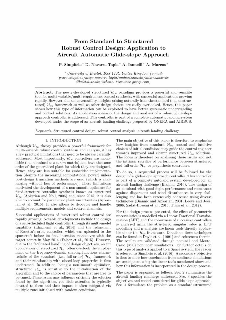
• Nominal performance of the linear system, which issatisfied if ||M(s)||∞ < 1 with ∆ = 0. As mentionedin Sec. 4, it corresponds to having the multi-channelsingular values of P (s) appropriately scaled by theinput weights Wc(s) and Wd(s) and bounded bythe inverse weights W−1

s (s) and W−1a (s). This is

visualised for the different controllers in Fig. 3;• Robust performance of the linear system, which is sat-

isfied if the same control requirements are fulfilled forall the allowable parametric uncertainties ||∆||∞ ≤ 1.This is assessed through the structured singular valueµ(M), defined as:

µ(M) =1

min∆P{σ(∆P) : det(I−M∆P) = 0}

(6)

where ∆P corresponds to the block ∆ augmentedwith a fictitious complex uncertainty that closes theoutputs and inputs of M(s) and σ(∆P) represents itsmaximum singular values (Doyle et al., 1991). All therequirements are fulfilled in dispersed conditions ifand only if µ(M) < 1 and, even when this is notthe case, a controller that provides smaller values ofµ(M) is necessarily associated with better RobustPerformance (RP) properties.

-60

-30

0

To: vce

From: vcc

-60

-30

0

To: vze

-60

-40

-20

To: dT

c

10-4

100

104

-60

-40

-20

To: dE

cFrom: vzc

10-4

100

104

From: wx

10-4

100

104

From: wz

10-4

100

104

Kbase

Kst2

Ksti2

Krsti2

Krsti3

Frequency (rad/s)

Magnitude (

dB

)

Fig. 3. Multi-channel singular values of the nominal plant (∆ = 0) against the design weights W−1s and W−1

a (in black)

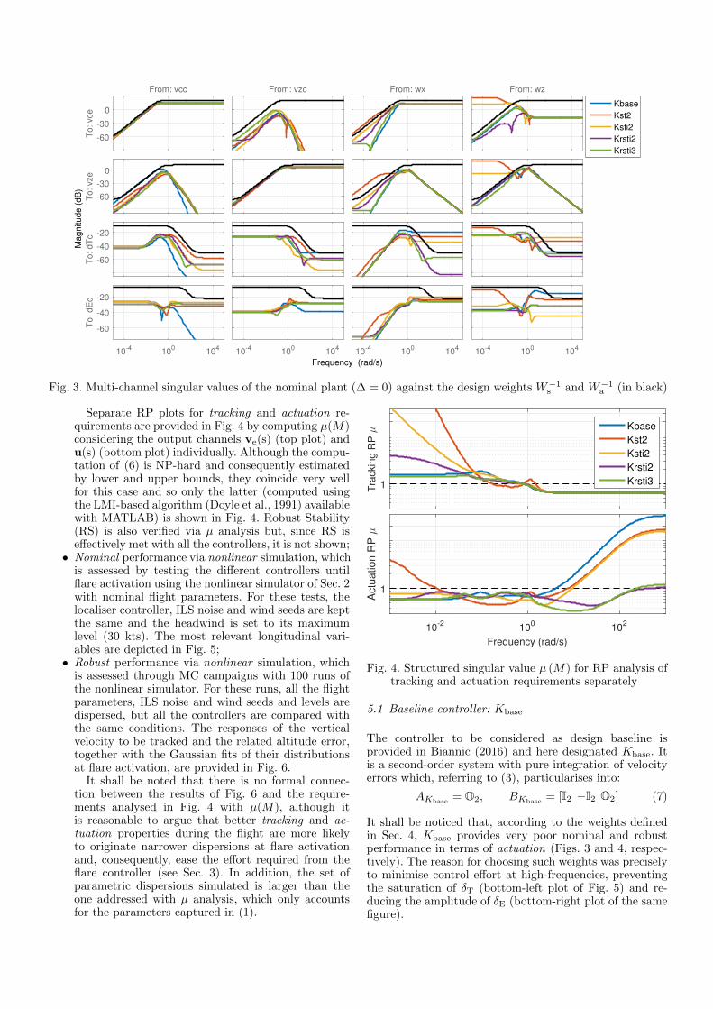
Separate RP plots for tracking and actuation re-quirements are provided in Fig. 4 by computing µ(M)considering the output channels ve(s) (top plot) andu(s) (bottom plot) individually. Although the compu-tation of (6) is NP-hard and consequently estimatedby lower and upper bounds, they coincide very wellfor this case and so only the latter (computed usingthe LMI-based algorithm (Doyle et al., 1991) availablewith MATLAB) is shown in Fig. 4. Robust Stability(RS) is also verified via µ analysis but, since RS iseffectively met with all the controllers, it is not shown;• Nominal performance via nonlinear simulation, which

is assessed by testing the different controllers untilflare activation using the nonlinear simulator of Sec. 2with nominal flight parameters. For these tests, thelocaliser controller, ILS noise and wind seeds are keptthe same and the headwind is set to its maximumlevel (30 kts). The most relevant longitudinal vari-ables are depicted in Fig. 5;• Robust performance via nonlinear simulation, which

is assessed through MC campaigns with 100 runs ofthe nonlinear simulator. For these runs, all the flightparameters, ILS noise and wind seeds and levels aredispersed, but all the controllers are compared withthe same conditions. The responses of the verticalvelocity to be tracked and the related altitude error,together with the Gaussian fits of their distributionsat flare activation, are provided in Fig. 6.

It shall be noted that there is no formal connec-tion between the results of Fig. 6 and the require-ments analysed in Fig. 4 with µ(M), although itis reasonable to argue that better tracking and ac-tuation properties during the flight are more likelyto originate narrower dispersions at flare activationand, consequently, ease the effort required from theflare controller (see Sec. 3). In addition, the set ofparametric dispersions simulated is larger than theone addressed with µ analysis, which only accountsfor the parameters captured in (1).

1Tra

ckin

g R

P µ

Kbase

Kst2

Ksti2

Krsti2

Krsti3

10-2

100

102

Frequency (rad/s)

1

Actu

ation R

P µ

Fig. 4. Structured singular value µ (M) for RP analysis oftracking and actuation requirements separately

5.1 Baseline controller: Kbase

The controller to be considered as design baseline isprovided in Biannic (2016) and here designated Kbase. Itis a second-order system with pure integration of velocityerrors which, referring to (3), particularises into:

AKbase= O2, BKbase

= [I2 −I2 O2] (7)

It shall be noticed that, according to the weights definedin Sec. 4, Kbase provides very poor nominal and robustperformance in terms of actuation (Figs. 3 and 4, respec-tively). The reason for choosing such weights was preciselyto minimise control effort at high-frequencies, preventingthe saturation of δT (bottom-left plot of Fig. 5) and re-ducing the amplitude of δE (bottom-right plot of the samefigure).

55

65

75

Vc (

m/s

)

-4

-2

0

Vz (

m/s

)

0.8

1

1.2

Nz (

g)

Kbase Kst2 Ksti2 Krsti2 Krsti3

-2

0

2q

(d

eg

/s)

0 50 100

Time (s)

1

1.1

1.2

dT

0 50 100

Time (s)

-10

0

10

dE

(d

eg

)

Fig. 5. Nonlinear simulation under nominal conditions andmaximum headwind level until flare activation

5.2 First structured controller: Kst2

This control design, Kst2, is obtained applying structuredH∞ and the requirements of Sec. 4 to the nominal plant(∆ = 0) and using a set of random second-order controllersas initial conditions. Note that this is not a structured con-troller per se; structured H∞ was employed to constrainits order but not its architecture at this point.

Poor nominal and robust performance with respect towx(s) and wz(s) disturbance inputs are observed in Figs. 3and 4, respectively. This, when tested with the nonlinearsimulator, leads to an unacceptable tracking in Fig. 6.

5.3 Structured controller initialised with H∞: Ksti2

The objective of this control design, Ksti2, is preciselyto obtain more meaningful singular value responses byavoiding the random initialisation employed for Kst2. Toachieve this while keeping the design choices of Sec. 5.2 (i.e.using ∆ = 0 and the same H∞ objectives), the followinggenerally-applicable synthesis procedure is proposed:

(1) A standard H∞ controller is computed. This con-troller is of order 10 (see Sec. 4) and originates||M(s)||∞ = 1.00;

(2) A controller is generated reducing the standard H∞design to order 2 via balanced truncation;

(3) The same structured problem of Sec. 5.2 is solved, butusing the reduced controller as single initial condition.The solution is Ksti2, which yields ||M(s)||∞ = 1.07.

Without a proper initialisation, systune would converge tosolutions similar to Kst2. However, due to the manipula-tion proposed above, the performance achieved with Ksti2

is substantially better (see Figs. 3 and 6).

Nonetheless, because Ksti2 is specifically tuned for thenominal plant, it is still very sensitive to model uncer-tainties as indicated by the plots of µ(M) in Fig. 4.

Fig. 6. Results of equal MC runs until flare activation(black lines show the nominal response without wind)

5.4 Structured controller retuned for the LFT: Krsti2

This glide-slope controller, Krsti2, is designed followingthe exact same steps of Sec. 5.3 (i.e., initialising witha reduced standard H∞ controller), but replacing thenominal plant with the full LFT, since systune is currentlyable to account for parametric uncertainties (Apkarianet al., 2015).

As expected, using the LFT for synthesis allows to sig-nificantly improve the robust performance of the system,especially in terms of actuation (Fig. 4). However, if doneinattentively, this may come at the expense of a loss ofnominal performance, as verified by the degraded trackingof vc in Figs. 3 and 5 (recall that the calibrated airspeedshould be kept constant during the approach). This is thenreflected into an erratic distribution of altitude for Krsti2

at flare activation, in Fig. 6.

5.5 Added-structure controller retuned for the LFT: Krsti3

As verified in Sec. 5.4, the controller developed thereinfor the LFT has to be retuned for better performance.To do so, the same synthesis steps were repeated usingmodified design weights. However, it soon became clearthat the optimiser would easily converge to solutions withinadequate singular value responses of vcc(s) → δTc(s),although very good in the channels related to δEc(s). Thisis an indication that a controller with more structure isneeded to meet the desired requirements.

Therefore, the original weights of Sec. 4 are kept butone extra degree-of-freedom is added to the controller.Nonetheless, this extra state is not added randomly. In-stead, the ability of structured H∞ to specify which pa-rameters or blocks are free to be optimised is exploited inorder to keep the very good behaviour of δEc(s) while onlytuning the other channel. Referring to (3), this is done byinitialising Krsti3 based on Krsti2, with:

AKrsti3 =

A∗red(Krsti2) 0∗ 0∗

0AKrsti20

, BKrsti3 =

[B∗red(Krsti2)

BKrsti2

]

CKrsti3 =

[C∗δT red(Krsti2) 0∗ 0∗

0 CδEKrsti2

]DKrsti3

=

[D∗δTKrsti2

DδEKrsti2

]In these expressions, the superscript ∗ denotes the blocksand parameters that are free to be tuned and the subscriptred(Krsti2) represents the reduction of the δTc(s) channelof Krsti2 to order 1 via balanced truncation. It shall benoted that, although the dynamics of δEc(s) are unaffected,the δTc(s) channel is able to use its states.

Once optimised, the impact of the extra dynamics of Krsti3

is clearly verified in Fig. 3, with smoother responses, espe-cially in the vce(s) channel. Consequently, an improvementof nominal performance is also observed on the otherchannels, which is then confirmed via nonlinear simulation(Fig. 5). Although similar to the other controllers concern-ing nominal tracking, Krsti3 is able to reduce significantlythe high-frequency actuation, which results in lower pitchrate q and also load factor Nz oscillations. Relative tothe other controllers, this comes at the cost of only oneadditional degree-of-freedom.

Regarding robust performance (Fig. 4), Krsti3 surpasses allthe other controllers in terms of actuation and tracking,which is proved via the MC analysis of Fig. 6. In fact,although the controllers generate a similar vertical veloc-ity distribution, the smallest integrated error with Krsti3

clearly makes it the best performing controller, with thenarrowest altitude error distribution at flare activation.This then facilitates the action of the flare controller (recallSec. 3) in the succeeding phase of the automatic landing.

6. CONCLUSIONS

This paper illustrated the application of structured H∞optimisation to the synthesis of a glide-slope approachcontrol system with good robustness against changingaircraft conditions and strong wind gusts. The effectsof varying aircraft conditions are captured via a LinearFractional Transformation (LFT) model and the windgusts are modelled as external disturbances.

Moreover, with this application, it was demonstrated howdesign choices that are easily overlooked can be decisive forthe quality of the solution found. Particular emphasis wasplaced on the benefits of employing a standard H∞ designto initialise the structured H∞ optimiser and of exploitingthe latter’s ability to specify which parameters are freeto be tuned. A generally-applicable synthesis procedurebased on the former was also proposed in Sec. 5.3.

During the design process, the aforementioned choiceswere taken and justified based on combined linear anal-yses and nonlinear simulations for both nominal and dis-persed flight conditions. Regarding the latter, robustnessassessments in the linear domain are performed using thestructured singular value µ and validated via nonlinearMonte-Carlo campaigns. All the insights provided by thesetools are complementary and crucial for the developmentof a successful control system.

The design of well-performing and robust aircraft auto-matic landing systems is indeed a very complex problemand the most effective way to tackle it is by addressing itscompounding control modes (glide-slope, localiser, flare)separately. The glide-slope approach controller Krsti3 isnow integrated in a complete autoland system developedfor the aircraft landing challenge.

REFERENCES

Apkarian, P., Dao, M., and Noll, D. (2015). Parametricrobust structured control design. Transactions on Au-tomatic Control, 60(7), 1857–1869.

Apkarian, P. and Noll, D. (2006). Nonsmooth H∞ Synthe-sis. Transactions on Automatic Control, 51(1), 71–86.

Biannic, J.M. (2016). Nonlinear Civilian Aircraft LandingBenchmark. Technical note included in the bench-mark package available with the SMAC toolbox athttp://w3.onera.fr/smac/aircraftModel.

Biannic, J.M. and Apkarian, P. (2001). A new approachto fixed-order H∞ synthesis: Application to autolanddesign. In The 2001 AIAA Guidance, Navigation, andControl Conference and Exhibit. Montreal, Canada.

Biannic, J.M. and Roos, C. (2015). Flare control lawdesign via multi-channel H∞ synthesis: Illustration ona freely available nonlinear aircraft benchmark. In The2015 American Control Conference. Chicago, IL.

Doyle, J., Packard, A., and Zhou, K. (1991). Review ofLFTs, LMIs and µ. In The 30th IEEE Conference onDecision and Control. Brighton, UK.

Falcoz, A., Pittet, C., Bennani, S., Guignard, A., Bayart,C., and Frapard, B. (2015). Systematic design methodsof robust and structured controllers for satellites. CEASSpace Journal, 7(3), 319–334.

Gahinet, P. and Apkarian, P. (2011). Structured H∞Synthesis in MATLAB. In The 18th IFAC WorldCongress. Milan, Italy.

Iannelli, A., Simplıcio, P., Navarro-Tapia, D., and Marcos,A. (2017). LFT Modeling and µ Analysis of theAircraft Landing Benchmark. In The 20th IFAC WorldCongress. Toulouse, France.

Lhachemi, H., Saussie, D., and Zhu, G. (2014). A Robustand Self-Scheduled Longitudinal Flight Control System:a Multi-Model and Structured H∞ Approach. In TheAIAA SciTech 2014 Conference. National Harbor, MD.

Looye, G. and Joos, H.D. (2006). Design of AutolandController Functions with Multiobjective Optimization.J. of Guidance, Control, and Dynamics, 29(2), 475–484.

Navarro-Tapia, D., Simplıcio, P., Iannelli, A., and Mar-cos, A. (2017). Robust Flare Control Design usingStructured H∞ Synthesis: a Civilian Aircraft LandingChallenge. In The 20th IFAC World Congress. Toulouse,France.

Sadat-Hoseini, H., Fazelzadeh, S., Rasti, A., and Mar-zocca, P. (2013). Final Approach and Flare Control ofa Flexible Aircraft in Crosswind Landings. Journal ofGuidance, Control, and Dynamics, 36(4), 946–957.

Simplıcio, P., Bennani, S., Marcos, A., Roux, C., andLefort, X. (2016). Structured Singular-Value Analysisof the Vega Launcher in Atmospheric Flight. Journal ofGuidance, Control, and Dynamics, 39(6), 1342–1355.

Theis, J., Ossmann, D., and Pfifer, H. (2017). RobustAutopilot Design for Crosswind Landing. In The 20thIFAC World Congress. Toulouse, France.