Embed Size (px)
Citation preview

1
From-Region Visibility andRay Space Factorization
Daniel Cohen-OrTel-Aviv University
Overview
Short introduction to the problemDual Space & Parameter/Ray SpaceRay space factorization (SIGGRAPH’03)
From Point Visibility
Input:– Large scene– Viewpoint
Output:– Set of visible objects from the
viewpoint
From the blue point only the blue objects are visible
From Point Visibility
From-region Visibility From Region Visibility
A much harder problem:The red objects are now visible by
the blue rays4D problem for 3D scenes
Compute the set of objects which partially visible from anywhere in the viewcell
2
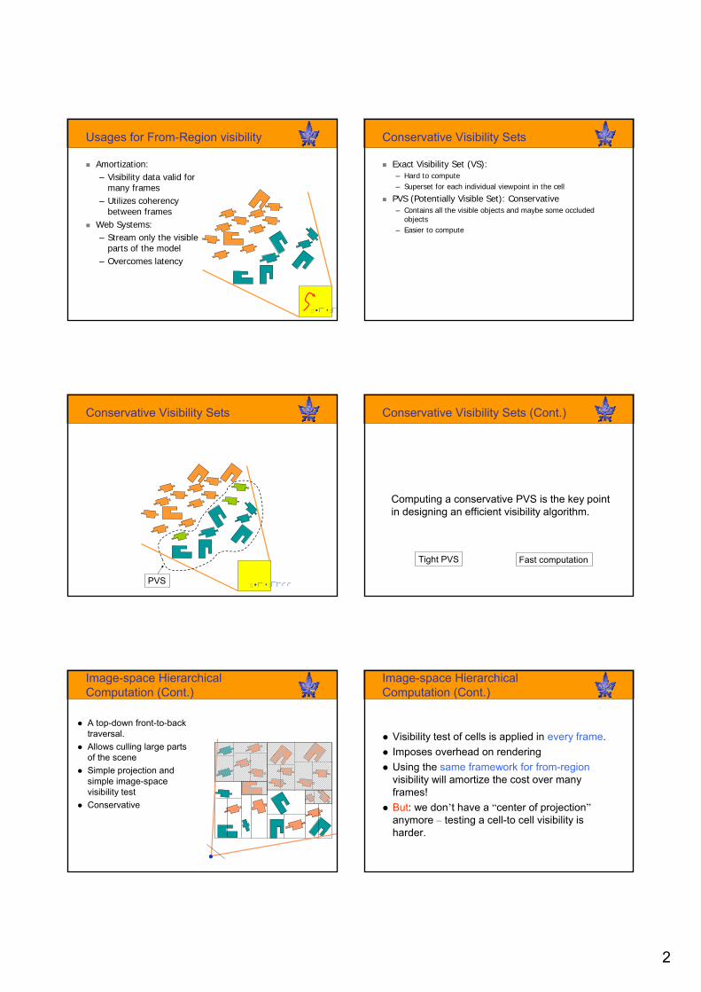
Usages for From-Region visibility
Amortization: – Visibility data valid for
many frames– Utilizes coherency
between framesWeb Systems:– Stream only the visible
parts of the model– Overcomes latency
iew c
Conservative Visibility Sets
Exact Visibility Set (VS):– Hard to compute– Superset for each individual viewpoint in the cell
PVS (Potentially Visible Set): Conservative– Contains all the visible objects and maybe some occluded
objects– Easier to compute
Conservative Visibility Sets
iew cellPVS
Conservative Visibility Sets (Cont.)
Computing a conservative PVS is the key point in designing an efficient visibility algorithm.
Tight PVS Fast computation
A top-down front-to-back traversal.Allows culling large parts of the sceneSimple projection and simple image-space visibility testConservative
Image-space Hierarchical Computation (Cont.)
Image-space Hierarchical Computation (Cont.)
Visibility test of cells is applied in every frame.Imposes overhead on renderingUsing the same framework for from-regionvisibility will amortize the cost over many frames!But: we don’t have a “center of projection”anymore – testing a cell-to cell visibility is harder.

3
Straightforward solution: Sampling
Problem:– Is the green object visible from
the viewcell?Solution:
– Sample some points from within the viewcell
– Test if the green object is visible from each sampled point
Con:– Not conservative– Slow!
ה View cell
Strong Occlusion Test
Algorithm:– Find objects occluded by a single
convex occluder– Mark only such objects as hidden
Pro:– Conservative solution– Fast
Con:– Objects may be occluded only by a
combination of other objects (Weakly Occluded)
– Large viewcells
ה
Umbrae of occluders
Positive UmbraNegative Umbra
Occluder Fusion
Visibility preprocessing with occluder fusion for urban walkthroughs – P. Wonka et.al. EGRW’ 2000
Virtual Occluder …– V. Koltun at.el. EGRW’ 2000
Conservative Volumetric Visibility with Occluder Fusion– G. Schaufler et.al. SIGGRAPH’2000
Visibility Preprocessing using Extended Projections– F. Durand et.al. SIGGRAPH’2000
Occluder Fusion – Key Idea
Merge umbrae that intersectFuse small umbrae into larger aggregated umbrae
View cell
Intersecting Umbrae - problem
Doesn’t capture all the cases of occluder fusion
View cell

4
Ray (parameter) space techniques
All rays hitting an object define a footprint in parameter space.
Boolean set operations on footprints determine visibility.
Exact - captures all the cases of occluder fusion.
Simple Dual Space
Simple duality transformation in 2D:
– L : y = ax+b L*: (-a,b) – p: (a,b) p* : y = -ax+b
Primal Plane
y = ax+b
Dual Plane
(-a,b)
Simple Dual Space
All lines passing through a point are mapped to a line
Primal Plane Dual Plane
Basic Dual Space (Cont.)
The lines that intersect a line-segment produce a double-wedge in dual-space
We can encode all the lines that intersect a segment into some footprint in dual-space
p
qL
L*
p*
q*
Parameter Space Footprint
Is segment A mutually visible from segment B ?– WA ∩ WB describes all possible sight-lines– The union of footprints of the occluder segments is the aggregated
occlusion of these segments
A
B
WA ∩ WB
Parameter space - discussion
Advantages:– Easy to implement with Boolean set operations– Great for occluder fusion – provides exact solution
Problems:– The footprint is unbounded – can’t be discretized and
implemented in hardware– No simple extension to 3D rays

5
Hardware Accelerated[Koltun, Cohen-Or and Chrysanthou, EGRW2001]
Put a plane lying on the viewcell A and the target cell BFor 2.5D occluders: A & B are mutually visible iff their upper rims are mutually visibleReduces the 2.5D problem into planar visibility test
BAA B
s2
s1
Parameter Ray Space
S1
S2
S2
S1
0,0
1
11
10
0ℜ2
Ray Space
Parameter Ray Space
S1
S2
S2
S1
0,0
1
11
10
0ℜ2
Ray Space
Footprint
Render all the footprint polygons onto parameter spaceCheck whether the frame buffer is fully coveredConservativeness - draw only fully covered pixels
0 1
1s2s2
s10 1
1
s1
s2 s2
s1
s1
Hardware Accelerated Occlusion Test
Discussion
This parameterization is boundedCan be efficiently used with graphics hardware
The parameterization is valid only within the shaft.Need to construct different parameter space for each occludee –which means each occluder is processed many times. 2.5D occluders only.Conclusion: we need something better…
Ray Space Factorization (Siggraph’03)
Use a bounded parameter spaceOne global parameter spaceEach occluder is processed onceSupport 3D scenesFast using graphics HW

6
viewcell
The dimensionality of the from-region problem
From-Region visibility is 4D
viewcell
From-Region visibility is 4D
A ray exists the viewcell through a 2D surface and enters the target region through a 2D surface
The dimensionality of the from-region problem
Horizontal direction Vertical direction
We factor the 4D visibility problem into horizontal and vertical components
Our Factorization
v
u
Lumigraph/light-field
A 2D grid of 2D images
Our Main Contribution
Our factorization:
•Exploits vertical coherence
•Maps to the graphics cards t
R
R ‘
Horizontal direction
Vertical direction
Vertical umbra
Algorithm Overview
Per Object:•Parameterization of vertical slices•Umbra encoding

7
Algorithm Overview (Cont.)
Top-down, front-to-back traversal of a KD-tree hierarchyObjects in visible leafs serve as occluders
Parameterization in 2D
Two concentric squaresParameters (s,t) are associated with the inner and outer squares ( 0<s,t<1)
s=0t=0
1/4
1/2 s
t
1/23/4
1/4
3/4
s=01/4
1/4 q
1/23/4
A Footprint of a Segment in 2D
1/4 1/2 3/4 1
)4/1(qt
)2/1(qt)4/1(qt
)2/1(qt
0
A footprint of a 2D segment is several 2D polygons
s
t
Extension to 3D
2D solution is not enough– Can’t tell whether an object is really
occludedPlucker Coordinates– The curse of dimensionality– Very slow, no hardware realization
[Bittner and Prikryl 01, Nirenstein02]
s
t
Within a Vertical Slice Within a Vertical Slice
A ray that leaves the viewcell has a 2D horizontal directionEach horizontal direction (s,t) defines a vertical-sliceWithin the slice the ray has a 2D vertical direction

8
Horizontal direction Vertical direction
ts ts
Horizontal and Vertical directions
We need to encode more than a single value per slice…
v
s
t
Parameter Space
viewcell
directio
nal
umbra
Vertical slice P(s,t)
Umbra Encoding
Encode supporting and separating angles
viewcell
Directionalaccumulatedumbra
Vertical slice P(s,t)
tα
bα
tβ
bβ
Testing Visibility
In parallel (in all slices) test occlusion by comparing supporting angles
viewcell
Umbrae Merging
Augment (fuse) the aggregated umbra if the directional umbra intersects
viewcell
Umbrae Merging (Cont.)
Otherwise, create another umbra entry. If there are too many discard it.
v
s
t
),( 00 ts
s
t
(s,t) plane (s,t,v) plane Primal Space
0v
),( 00 ts
),,( 000 vts
A simple case
To make it clearer, let’s look at a simpler case.
Here we just encode the top-elevation angle

9
Merging Umbrae (within the slice)
1
2
4
5
6
7
– Process objects in front-to-back order– Maintain the aggregated umbrae
viewcell
3
Merging Umbrae
1
2
4
5
6
7
viewcell
3
– Process objects in front-to-back order– Maintain the aggregated umbrae
Merging Umbrae
2
4
5
6
7
viewcell
1 3
– Process objects in front-to-back order– Maintain the aggregated umbrae
Merging Umbrae
2
3
4
5
6
7
viewcell
1
– Process objects in front-to-back order– Maintain the aggregated umbrae
Merging Umbrae
2
4
5
6
7
viewcell
31
– Process objects in front-to-back order– Maintain the aggregated umbrae
Merging Umbrae
2
4
5
6
7
viewcell
31
– Process objects in front-to-back order– Maintain the aggregated umbrae

10
Merging Umbrae
2
4
5
6
7
viewcell
31
– Process objects in front-to-back order– Maintain the aggregated umbrae
Merging Umbrae
2
4
5
6
7
viewcell
31
– Process objects in front-to-back order– Maintain the aggregated umbrae
Merging Umbrae
2
4
5
6
7
viewcell
31
– Process objects in front-to-back order– Maintain the aggregated umbrae
Merging Umbrae
2
4
5
6
7
viewcell
31 Segments 6 and 7 can be identified as occluded
– Process objects in front-to-back order– Maintain the aggregated umbrae
Pixel-shader
Performs all the directional operations simultaneously over all the pixels of the occluder footprint.The pixel resolution defines the degree of conservativeness.
A Multi-layer Occlusion Map
Each pixel is associated with a series of supporting and separating angles pairs used by the pixel-shaderoperationThe number of umbrae is limited

11
A Single Aggregated Umbra
Maintain a single aggregated umbraThe algorithm is still conservative
Final aggregated umbra using a single aggregateFinal aggregated umbra using two aggregates
24
5
6
7
viewcell
31
24
5
6
7
viewcell
31
A Single Value – 2.5D scene
Aggregated umbrae always intersectFast on common graphics card
2.5D Example
The red skyscrapers (left) have large top supporting anglesTheir red footprints are visible => the skyscrapers themselves are visible
Primal Space Parameter Space
A top-down front-to-back traversal.Allows culling large parts of the sceneSimple projection and simple image-space visibility testConservative
Image-space Hierarchical Computation
A top-down front-to-back traversal.NOT-Simple projection and simple ray-space visibility testConservative
Ray-space Hierarchical Computation
Random Urban Model Box Field ModelVienna 2000 Model
Results

12
Results – Random Urban Model Results – Box Field Model
Results – Vienna 2000 Model The End
Thank You
Preliminary results
The algorithm is extremely fast if implemented with hardware support.Even faster with new hardware (pixel shader operations, occlusion flag)
6687101778951,308.7K
622663164834325.9K
44747612360580.1K
3203418743318.8K
3513741014794.7K
ReadTotal timeFootprint times
(ms)Total Times
(ms)No. of
trapezoidsFrame Buffer
Performance Table

13
The End
(a) (b)City with T & H shaped buildings along a street. (a) is taken from within the view-cell (in green) and (b) froma birds eye (gray buildings are hidden)
Non-linearity of parameterization
viewcell
L(s,t)
H(s,t)α ),(),(αtan
tsLtsH
=
We approximate this rational function by a linear function
Handling arbitrary triangles
s=0t=0
1/4
1/21/23/4
1/4
3/4
Horizontal component: parameterize each visible edge
Inside directional slice: as before!


![Visibility Sampling on GPU and Applications · visibility sampling [WWZ06], ray mutations are used to sample visibility where it is most relevant. The method is very fast and uses](https://img.dokumen.tips/doc/110x75/6146cdc6f4263007b13569b9/visibility-sampling-on-gpu-and-applications-visibility-sampling-wwz06-ray-mutations.jpg)