Embed Size (px)
Citation preview
FROM PQCD TO NEUTRON STARS: MATCHING
EQUATIONS OF STATE TO CONSTRAIN GLOBAL
STAR PROPERTIES
by
TYLER GORDA
B.S., Rutgers, the State University of New Jersey, 2011
M.S., University of Colorado Boulder, 2014
A thesis submitted to the
Faculty of the Graduate School of the
University of Colorado in partial fulfillment
of the requirements for the degree of
Doctor of Philosophy
Department of Physics
2016

This thesis entitled:From pQCD to neutron stars: matching equations of state to constrain global star properties
written by Tyler Gordahas been approved for the Department of Physics
Prof. Paul Romatschke
Prof. Anna Hasenfratz
Date
The final copy of this thesis has been examined by the signatories, and we find that both thecontent and the form meet acceptable presentation standards of scholarly work in the
above-mentioned discipline.

iii
Gorda, Tyler (Ph.D., Physics)
From pQCD to neutron stars: matching equations of state to constrain global star properties
Thesis directed by Prof. Paul Romatschke
The equation of state (EoS) of quantum chromodynamics (QCD) at zero temperature can be
calculated in two different perturbative regimes: for small values of the baryon chemical potential
µ, one may use chiral perturbation theory (ChEFT); and for large values of µ, one may use per-
turbative QCD (pQCD). Each of these theories is controlled, predictive, and has much theoretical
development. There is, however, a gap for µ ∈ (0.97 GeV, 2.6 GeV), where these theories becomes
non-perturbative, and where there is currently no known microscopic description of QCD matter.
Unfortunately, this interval obscures the values of µ found within the cores of neutron stars (NSs).
In this thesis, we argue that thermodynamic matching of the ChEFT and pQCD EoSs is a
legitimate way to obtain quantitative constraints on the non-pertubative QCD EoS in this inter-
mediate region. Within this framework, one pieces together the EoSs coming from ChEFT (or
another low-energy description) and pQCD in a thermodynamically consistent manner to obtain
a band of allowed EoSs. This method trades qualitative modeling for quantitative constraints: one
attempts no microscopic characterization of the underlying matter.
In this thesis, we argue that this method is an effective, verifiable, and systematically im-
provable way to explore and characterize the interior of NSs. First, we carry out a simplified
matching procedure in QCD-like theories that can be simulated on the lattice without a sign prob-
lem. Our calculated pressure band serves as a prediction for lattice-QCD practitioners and will
allow them to verify or refute the simplified procedure. Second, we apply the state-of-the-art
matched EoS of Ref. [1] to rotating NSs. This allows us to obtain bounds on observable NS prop-
erties, as well as point towards future observations that would more tightly constrain the current
state-of-the-art EoS band. Finally, as evidence of the ability to improve the procedure, we carry out
calculations in pQCD to improve the zero-temperature pressure. We calculate the full O(g6 ln2 g)
iv
contribution to the pQCD pressure for nf massless quarks, as well as a significant portion of the
O(g6 lng) piece and even some of the O(g6) piece.

DEDICATION
This thesis is dedicated with warmest appreciation to my past teachers and educators of all
subjects.

vi
ACKNOWLEDGEMENTS
I would like to thank Paul Romatschke for his help and guidance over the last five years:
especially for his encouragements to participate in a variety of conferences and workshops and the
personal freedom he has given me to explore whatever physics I find interesting. I would also like
to thank Oscar Henriksson, Andrew Koller, and Paige Warmker for discussing many an interesting
physics topic over the years, and for helping me clarify many deep concepts. Many thanks as well
to Hans Bantilan, with whom I have also had many exciting and fruitful discussions, and who
constantly reminds me that mathematical clarity of thought not only has a place in physics, but is
vital to it. Lastly, I thank Aleksi Vuorinen, Ioan Ghisoiu, and Aleksi Kurkela for many stimulating
conversations about physics, which I look forward to continuing.
Finally, this thesis draws from two papers on which I have been an author. For those pa-
pers, I wish to acknowledge Gert Aarts, Tom DeGrand, Simon Hands, Yuzhi Liu, Marco Panero,
Paul Romatschke, Andreas Schmitt, and Aleksi Vuorinen for many helpful discussions and sug-
gestions.
CONTENTS
CHAPTER
1 GENERAL INTRODUCTION 1
2 THE PHASE DIAGRAM OF QCD 7
2.1 The general structure of QCD . . . . . . . . . . . . . . . . . . . . . . . . . . . . . . . . 7
2.2 The phase diagram of nuclear matter . . . . . . . . . . . . . . . . . . . . . . . . . . . . 10
2.2.1 Lattice QCD and the T-axis . . . . . . . . . . . . . . . . . . . . . . . . . . . . . 11
2.2.2 The µ-axis and phases in pQCD . . . . . . . . . . . . . . . . . . . . . . . . . . 12
3 PERTURBATIVE EXPLORATIONS OF QCD 16
3.1 PQCD at nonzero temperature and density . . . . . . . . . . . . . . . . . . . . . . . . 16
3.1.1 The partition function of a quantum field . . . . . . . . . . . . . . . . . . . . . 16
3.1.2 A derivation of the partition function for bosonic and fermionic fields . . . . 17
3.1.3 Changes to the Euclidean Lagrangians with a chemical potential . . . . . . . 21
3.1.4 The propagators an nonzero temperature and density . . . . . . . . . . . . . . 23
3.1.5 The pressure of interacting quantum fields at nonzero temperature and density 25
3.1.6 Feynman diagrams in thermal QCD . . . . . . . . . . . . . . . . . . . . . . . . 26
3.1.7 Restriction to zero temperature . . . . . . . . . . . . . . . . . . . . . . . . . . . 29
3.1.8 Ring/plasmon diagrams and their contribution to the pressure at zero tem-
perature . . . . . . . . . . . . . . . . . . . . . . . . . . . . . . . . . . . . . . . . 30
3.2 Low-energy effective theories of QCD . . . . . . . . . . . . . . . . . . . . . . . . . . . 34
viii
3.2.1 The HRG equation of state . . . . . . . . . . . . . . . . . . . . . . . . . . . . . 34
3.2.2 Chiral effective theory . . . . . . . . . . . . . . . . . . . . . . . . . . . . . . . . 37
4 MATCHING EQUATIONS OF STATE 43
4.1 Matching in QCD-like theories accessible to lattice QCD . . . . . . . . . . . . . . . . 44
4.1.1 pQCD equation of state . . . . . . . . . . . . . . . . . . . . . . . . . . . . . . . 46
4.1.2 Hadron resonance gas spectra in the QCD-like theories . . . . . . . . . . . . . 49
4.1.3 Matching the pQCD and HRG equations of state . . . . . . . . . . . . . . . . . 54
4.1.4 Results: HRG+pQCD matching . . . . . . . . . . . . . . . . . . . . . . . . . . . 55
4.1.5 Conclusions: HRG+pQCD matching . . . . . . . . . . . . . . . . . . . . . . . . 59
4.2 Kurkela et al. [1] matching: ChEFT to pQCD . . . . . . . . . . . . . . . . . . . . . . . . 60
5 NEUTRON STARS AND APPLICATIONS 62
5.1 The QCD EoS and the structure of NSs: overview . . . . . . . . . . . . . . . . . . . . 64
5.2 Global properties of NSs with QCD EoSs . . . . . . . . . . . . . . . . . . . . . . . . . 65
5.2.1 Non-rotating case . . . . . . . . . . . . . . . . . . . . . . . . . . . . . . . . . . . 66
5.2.2 General rotating case . . . . . . . . . . . . . . . . . . . . . . . . . . . . . . . . . 67
5.2.3 Conclusions: Applications to NS . . . . . . . . . . . . . . . . . . . . . . . . . . 73
6 HIGHER-ORDER TERMS IN THE PQCD PRESSURE AT ZERO TEMPERATURE 75
6.1 Higher orders for a single massless fermion . . . . . . . . . . . . . . . . . . . . . . . . 75
6.2 Higher-order terms for multiple massless fermions . . . . . . . . . . . . . . . . . . . . 79
6.3 Contribution of the two-loop self-energy . . . . . . . . . . . . . . . . . . . . . . . . . . 81
7 CONCLUSIONS 83
Bibliography 85
ix
APPENDIX
A PARTICLE TABLES 92

x
TABLES
TABLE
4.1 The ratios Tc/√σ and µc/
√σ for the theories analyzed in this section. Errors are
given by the number of significant figures. . . . . . . . . . . . . . . . . . . . . . . . . 57
A.1 The included particle spectrum in the two-color fundamental theory. . . . . . . . . . 92
A.2 The included particle spectrum in the four-color fundamental theory. . . . . . . . . . 93
A.3 The mesons, diquarks, and baryons in the four-color antisymmetric theory. (See
Table A.4 for remaining particles in this theory.) . . . . . . . . . . . . . . . . . . . . . 94
A.4 The included tetraquarks, di-mesons, and diquark-mesons in the four-color anti-
symmetric theory. (There is one of each of these particle types for each line in this
table.) Here, m, gS, and gI are the mass, total spin, and isospin degeneracies, re-
spectively. As noted above in Section 4.1.2, we need not determine how all of the
four-quark-object degrees of freedom break up into spin and isospin multiplets be-
cause of the mass degeneracy. . . . . . . . . . . . . . . . . . . . . . . . . . . . . . . . . 95

FIGURES
FIGURE
2.1 A cartoon of the QCD phase diagram. Taken from Ref. [14]. . . . . . . . . . . . . . . 10
4.1 Normalized pressure (left) and trace anomaly (right) at µ = 0 for the three-color,
three-massless-quark case from HRG+pQCD in comparison to lattice-QCD data
from the Budapest–Marseille–Wuppertal Collaboration [41] and the HotQCD Col-
laboration [42]. . . . . . . . . . . . . . . . . . . . . . . . . . . . . . . . . . . . . . . . . . 55
4.2 Normalized pressure (left) and trace anomaly (right) at µ = 0 for the two-color,
three-color, four-color fundamental, and four-color antisymmetric theories in HRG
+pQCD. Note that the T -axis has been scaled by the critical temperature (see main
text). . . . . . . . . . . . . . . . . . . . . . . . . . . . . . . . . . . . . . . . . . . . . . . 56
4.3 Normalized pressure (left) and trace anomaly (right) at T = 0 for the two-color,
three-color, four-color fundamental, and the four-color antisymmetric theories in
HRG+pQCD. Note that the µ-axis has been scaled by the critical chemical potential
(see main text). . . . . . . . . . . . . . . . . . . . . . . . . . . . . . . . . . . . . . . . . 57
4.4 Deconfinement-transition temperature Tc as a function of pion mass for the four-
color, antisymmetric theory in the µ = 0,ΛMS/√σ = 0.723 case. The straight line is a
fit to the results where matching could be performed, and defines the extrapolation
to the chiral limit (see main text). . . . . . . . . . . . . . . . . . . . . . . . . . . . . . . 58

xii
4.5 The speed of sound squared at T = 0 for the two-color, three-color, four-color fun-
damental, and the four-color antisymmetric theories in HRG+pQCD. Note that the
µ-axis has been scaled by the critical chemical potential (see main text). . . . . . . . 59
4.6 The allowed band of EoSs determined by Kurkela et al.[1], consisting of two- and
three-trope intermediate EoSs. From Ref. [1]. The ChEFT EoS is not shown on the
plot; it connects to the bands shown in the lower-left corner. In this plot, µB is
the baryon chemical potential, and P has been scaled by PSB, the Stefan–Boltzmann
pressure. . . . . . . . . . . . . . . . . . . . . . . . . . . . . . . . . . . . . . . . . . . . . 61
5.1 The allowed band of EoSs determined by Kurkela et al. [1], including the 2M mass
constraint. From Ref. [1]. The lines indicate individual constructed EoSs, and the
bold, dashed lines are tabulated in Ref. [1]. The crosses denote the largest value of µ
reached within a non-rotating NS constructed from each of the bold, dashed EoSs.
The ChEFT EoS is not shown on the plot; it connects to the bands shown in the
lower-left corner. Note that P has been scaled by PSB, the Stefan–Boltzmann pressure. 66
5.2 Mass vs. equatorial radius regions for non-rotating stars (horizontal stripes) and
mass-shedding stars (vertical stripes). The upper, checkered region is an overlap
between the non-rotating and mass-shedding regions. The lower, solid region is
only accessible to non-mass-shedding rotating NSs. . . . . . . . . . . . . . . . . . . . 69
5.3 The allowed mass–frequency region for all of the possible QCD EoSs. The inner,
solid region is allowed for every EoS, and the outer, checkered band shows where
the possible boundaries are for each EoS. The dashed line is the outer boundary of
the mass–frequency region for a sample EoS. Data points for NSs with f > 100Hz,
taken from a table in Ref. [85], are also plotted. . . . . . . . . . . . . . . . . . . . . . . 70
5.4 The region of allowed circumferential equatorial radius vs. frequency curves for a
1.4M star. . . . . . . . . . . . . . . . . . . . . . . . . . . . . . . . . . . . . . . . . . . . 71

xiii
5.5 The allowed region of moment of inertia vs. circumferential equatorial radius for
PSR J0737-3039A. . . . . . . . . . . . . . . . . . . . . . . . . . . . . . . . . . . . . . . . 72
5.6 A plot illustrating how much the QCD EoS band of Ref. [1] would be restricted by a
hypothetical measurement of I = 1.5× 1045 g cm2 with a precision of 10% for PSR
J0737-3039A. . . . . . . . . . . . . . . . . . . . . . . . . . . . . . . . . . . . . . . . . . . 73

CHAPTER 1
GENERAL INTRODUCTION
Quantum chromodynamics (QCD) is the microscopic theory of the strong nuclear force.
Fundamentally, it is a theory of interacting quarks and gluons, but by extension, it describes the
physics underpinning any objects composed of these elemental fields. Thus, in principle, the
theory of QCD describes a vast range of objects and phenomena. This ranges from phenomena
impacting our low-energy, everyday world (such as the structure and scattering of hadrons, the
binding of baryons to one another in nuclei, and the structure and properties of nuclei in atoms)
to much more exotic and energetic objects and processes (such as nuclear processes in the core
of typical stars, the structure and properties of compact neutron stars (NSs), and supernovae).
Unfortunately, in practice, most of these properties are not directly computable from the QCD path
integral itself (and even those that are require significant effort). The reason for this is that QCD
is non-perturbative at low energies. This means that only at high energies are the fundamental
quark and gluon fields useful descriptions of QCD: at the low energies relevant to our everyday
world, the weakly interacting degrees of freedom (i.e., the quasiparticles) are instead the baryons
and mesons. This change of degrees of freedom as one proceeds down in energy from colored
quarks and gluons to color-neutral hadrons is called confinement.
As a rule of thumb, perturbative (pQCD) calculations from the QCD path integral itself are
typically valid for energies much higher than the so-called ΛQCD scale, which is around 250MeV.
2
That is, roughly speaking, for energy scales E such that E ΛQCD, perturbation theory is valid.
This is, of course a very rough estimate, for what constitutes “much greater than” in the problem
is sometimes complicated or unclear. One can look at the running coupling constant αs(µ) and
see when this becomes of order one, but this just shifts the problem to defining what “of order
one” means. In any case, according to the Particle Data Group [2], αs(mZ) = 0.1148 ± 0.0007,
and this increases to αs(∼ 5 GeV) = 0.2 and αs(∼ 1.5 GeV) = 0.3. Thus, E ΛQCD more or less
translates to E > a few GeV. In what follows, we shall refer to this energy scale of a few GeV as the
perturbative scale: ΛpQCD.
On the low-energy side of the spectrum, the quasiparticles are hadrons. Again, precisely
what determines “low-energy” requires some care, but it is approximately 1.2 GeV. This scale cor-
responds roughly to the mass of the lightest non-pionic hadrons. This distinction between pions
and the rest of the hadrons is relevant because the pions are anomalously light for a reason: there
is a symmetry of the QCD Lagrangian that is not manifest in the ground state. This symmetry is
called chiral symmetry, and the aforementioned energy scale is referred to as the chiral symmetry
breaking scale ΛCSSB. At low energies, another perturbative theory exists called chiral effective
theory (ChEFT) which allows one to compute low-energy properties and processes within a con-
trolled framework [3, 4].
There is however, a pronounced gap in energies between ΛCSSB and ΛpQCD, which is out of
reach of any perturbative framework. To explore this region, one can resort to model Lagrangians
that incorporate some relevant phenomena, such as confinement or chiral symmetry breaking,
but in these models there is no controlled perturbative framework connected to the fundamental
physics. Within the context of the condensed matter of QCD, or thermal field theory (TQFT),
this non-perturbative region unfortunately obscures some very interesting physics. For example,
this region obscures the chiral and confinement transitions, meaning that researchers are unable
to study these transitions in a first-principled way throughout the entire phase plane. (There is
a non-perturbative numerical technique called lattice QCD, but its techniques are not currently
applicable outside of a narrow slice of the phase plane. This will be discussed in more detail in

3
Chap. 2.) In addition, at small temperatures (T ΛQCD) and large densities n or baryon chemical
(µ ΛQCD), this non-perturbative regime obscures the region of the phase diagram applicable to
the interiors of NSs.
On the one hand, this is a blessing: measurements of the properties of NSs can shed light
on a region of the QCD phase diagram that is inaccessible to current theoretical techniques. On
the other hand, NSs are extremely complex physical systems, combining fundamental QCD mi-
crophysics with thermodynamics and general relativity (and often extreme electromagnetism as
well), and thus extracting the properties of NSs from observations is very challenging. Often,
much theoretical modeling is necessary to perform this extraction, and since there is little theoret-
ical control over the models, there are large uncertainties. Some properties determined primarily
by the crust are understood in some detail, for the crust is of a low density and thus ChEFT or
other techniques can describe it well. We do have limited knowledge of possible exotic phases of
nuclear matter in the crust, and what effects crustal microphysics has on transport properties (see
Ref. [5, 6, 7] for reviews).
As one moves into the cores of NSs, however, direct theoretical knowledge is lost. There are
theoretical speculations of phase transitions to deconfined quark matter or even to the hypothe-
sized ground state of QCD, strange quark matter [8, 9], within the cores, but the models and ideas
in this region are, for the most part, phenomenological and not derived from QCD itself in a con-
trolled way. That is, most of the models used to predict the structure of NSs use microphysics that
is not connected rigorously to QCD.
However, there is a technique to reach the NS-region of the QCD phase diagram if one is not
interested in the microphysics: thermodynamic matching [10, 1, 11]. One can hope to constrain bulk
thermodynamic properties, such as the equation of state (EoS), along the entire µ-axis using the
two controlled perturbative regimes at low and high µ. The EoS in the non-perturbative middle
region will have to match the perturbative EoSs at the edges (meaning that the pressures of the two
phases must be equal at the matching points), and throughout, there are restrictions coming from
thermodynamic consistency and stability. For example, the energy density ε (and the pressure P)

4
must be monotonically increasing functions of µ, and on either side of a matching point, the stable
phase must be the one with the higher P. This simple prescription allows one to obtain a band
of permitted EoSs in the non-perturbative regime. With this in hand, one may investigate bulk,
global properties of NSs, including relations between the total massM; circumferential, equatorial
radius Re; frequency of rotation f; and the moment of inertia I. We stress that these predictions are
made essentially from the underlying QCD theory, and are thus constrained by first-principles,
controlled physics.
It is this remarkable story that we wish to tell in this thesis: one can constrain properties
of NSs governed by non-perturbative regimes of QCD by thermodynamically matching EoSs de-
termined by controlled, perturbative-QCD physics. There are three main goals that we wish to ac-
complish in this thesis, in addition to identifying thermodynamic matching as an approach to
real, physically interesting problems. First, we will show that this remarkably simplistic idea of
matching EoSs can be checked by lattice “QCD” in some QCD-like theories. This is an important
result, for it allows one to verify whether or not this simplistic, but seemingly powerful approach
can really achieve what it claims to achieve. Second, we will extend applications of the state-of-
the-art matched QCD EoS results of Kurkela et al. [1] and Fraga et al. [11] to rotating NSs. This
will give us insight into which astronomical observations would provide additional constraints
on the QCD EoS in the intermediate, non-perturbative regime (not to mention that this extension
will provide important bounds on global NS properties). Third, we will calculate higher-order
corrections to the zero-temperature pQCD EoS, which may be used in the future to conduct more
refined matching studies of the QCD EoS in the non-perturbative regime.
The structure of this thesis is as follows. In Chap. 2 we begin with the QCD phase diagram,
detailing which regions of the phase diagram permit direct theoretical investigation. We shall also
outline the various phases and phase transitions that have been theoretically proposed to exist,
as well as those which have been observed. In this chapter, we will be especially interested in
the T = 0 region of the phase diagram, for T = 0 is an excellent approximation for NSs after
their violent formation period [12, 13]. In Chap. 3, we discuss the perturbative approaches to

5
understanding QCD, and in particular, for calculating thermodynamic quantities. We provide a
comprehensive outline of thermal pQCD and explain how one may compute P as a perturbative
series in the strong coupling constant g =√4παs. In the process, we discuss a class of diagrams
known as the “plasmon” or “ring-sum” diagrams, and compute the g4 lng contribution to the
zero-temperature pQCD EoS, as an exercise. We also provide a brief introduction to low-energy
ChEFT in this chapter. Next, we take up the topic of EoS matching in Chap. 4. This chapter
investigates questions about the matching procedure itself. Specifically, we investigate if there are
ways to test if such a simple prescription actually works, using exotic “QCD-like” theories. In
addition, we describe the current state-of-the-art matching procedure carried out in Refs. [1, 11].
Chap. 5 contains an brief overview of NSs, including a general discussion of NS structure within
the framework of general relativity. This chapter also includes a survey of connections between
the EoS band of Kurkela et al. [1] and global properties of rotating NSs. We examine the bounds on
observable NS properties that follow from the EoS band, and we discuss future observations that
can further constrain the band. Finally, in Chap. 6, we present improvements to the pQCD EoS
at T = 0. We present a derivation of the O(g6 ln2 g) term in the pressure for an arbitrary number
nf of massless quarks from the plasmon sum terms, as well as parts of the O(g6 lng) and O(g6)
terms. Finally, Chap. 7 contains our conclusions.
Let us now begin our approach towards the aforementioned goals with a survey of the QCD
phase diagram.
Notation
A brief word on notation in this thesis: we will work in the mostly minus convention, with
the Minkowski metric ηµν = diag(+1, −1, −1, −1). Four-vectors shall be denoted Pµ, with com-
ponents Pµ = (p0,~p). We shall denote the number of flavors of quarks as nf, and when we gener-
alize to QCD-like theories, N shall denote the number of possible colors for a quark in the funda-
mental representation (e.g. SU(N)). Gluonic color indices shall be drawn from the beginning of the

6
Latin alphabet: a, b, c, . . . ; flavor indices from the middle of the Latin alphabet: f, g, h, . . . ; and
quark color indices from the beginning of the Greek alphabet: α, β, γ, . . . . Space-time indices
shall be drawn from the middle of the Greek alphabet: µ, ν, ρ, . . . . In this thesis, Boltzmann’s
constant k, Planck’s reduced constant h, and the speed of light c will be set equal to one through-
out.

CHAPTER 2
THE PHASE DIAGRAM OF QCD
In this chapter, we present a survey of the phase diagram of QCD, with an emphasis on the
µ-axis. We will start with a brief overview of QCD itself (more details will be given in Chap. 3),
and mention which parts of the phase diagram are accessible by direct calculations. This will
consist of three different regions: first, regions on and near the T -axis, which are accessible to
lattice-QCD techniques; second, the T ΛpQCD region on and near the T -axis and the µ ΛpQCD
region on and near the µ-axis, which are accessible by pQCD; and third, the T ΛCSSB, µ ΛCSSB
region, accessible by ChEFT. In these regions, we will review what is known, with emphasis on
the thermodynamic phases. We will also detail the main phase-transition regions, including those
that are not well-understood (e.g., the confinement-deconfinement and chiral symmetry breaking
transitions). We will finish with a focus on the non-perturbative region on and near the µ-axis,
which is relevant to NSs.
2.1 The general structure of QCD
QCD is a theory of nf = 6 flavors (f = u, d, s, c, b, t) of massive quarks with color indices
α = 1, 2, 3 interacting via an SU(3) gauge boson (the gluon) with color indices a = 1, 2, . . . , 8. We

8
shall depict these fields as ψαf and Aaµ respectively. The Lagrangian is
LQCD =∑f
ψαf
(δαβ
(iγµ∂µ −mf
)+ gγµAaµT
aαβ
)ψβf −
1
4FaµνF
aµν, (2.1)
where here and in what follows, repeated color indices are always summed over. Here, γµ are the
Dirac gamma matrices, g is the gluon coupling constant,mf is the mass of the fth quark,ψ = ψ†γ0,
Fµν is the gluonic field strength tensor
Faµν = ∂µAaν − ∂νA
aµ − gfabcAbµA
cν, (2.2)
with fabc to be defined below, and Ta•• are the generators of SU(3) in the same (fundamental)
representation as the quarks (as can be seen from the lower indices in Eq. (2.1)). In what follows,
we shall denote a general representation as R. Since in Chap. 4, we shall be considering different
fermionic representations, we will take a moment here to remind the reader of the properties of
these TaR . Regardless of the representation (i.e., range of the lower indices) these matrices satisfy
commutation relations
[TaR , TbR ] = i fabcTcR, (2.3)
where the fabc are the structure constants of SU(3). The fabc are completely antisymmetric and
are defined by
f111 = 1, f147 = f165 = f246 = f257 = f345 = f376 =1
2, f458 = f678 =
√3
2. (2.4)
For the fundamental representation of SU(3), the generators are given by Taf = λa/2where the λa
are the Gell-Mann matrices:
λ1 =
0 1 0
1 0 0
0 0 0
, λ2 =
0 − i 0
i 0 0
0 0 0
, λ3 =
1 0 0
0 −1 0
0 0 0
, (2.5)
λ4 =
0 0 1
0 0 0
1 0 0
, λ5 =
0 0 − i
0 0 0
i 0 0
, (2.6)

9
λ6 =
0 0 0
0 0 1
0 1 0
, λ7 =
0 0 0
0 0 − i
0 i 0
, λ8 =1√3
1 0 0
0 1 0
0 0 −2
. (2.7)
In the fundamental representation, the Taf are normalized such that
Tr (Taf Tbf ) = Tfδ
ab, (2.8)
TaαβTaβγ = Cfδαγ, (2.9)
facdfbcd = CAδab, (2.10)
with Tf = 12 , Cf = 32−1
2·3 = 43 , and CA = 3. Eq. (2.8) and Eq. (2.9) can be extendend to an arbitrary
representation R; in that case, these equations define new constants TR and CR.
A few words about these factors are in order here. First, they are frequently written in terms
of N for a general SU(N) gauge theory, it which case one has Tf = 12 , Cf = N2−1
2N , and CA = N.
Secondly, the quark fields ψαf are commonly combined into a single quark flavor vector ~ψα. In
this case, the flavor index f disappears from the fields and appears in the Tf: Tf = nf2 instead in
this case, since the trace in Eq. (2.8) will also trace over the flavor index as well. Lastly, the “A”
in Eq. (2.10) stands for “adjoint”. The generators of the adjoint representation are defined by the
structure constants:
(TaA)bc = − i fabc. (2.11)
(Note that for the structure constants, whether an index is up or down makes no difference.) This
definition means that Eq. (2.10) is a special case of the generalized Eq. (2.9).
One final note must be made about the general structure of QCD. Although there are indeed
nf = 6 flavors of quarks in nature, only nf = 3 are ever probed at zero temperature in nature. As
will be discussed in the following section, in NSs, the quark chemical potential µq is always much
below the mass of the c quark. This means that only the three lightest quarks (u, d, s) are active
within dense nuclear matter.

10
FIGURE 2.1: A cartoon of the QCD phase diagram. Taken from Ref. [14].
2.2 The phase diagram of nuclear matter
In Fig. 2.1 we present a cartoon of the phase diagram of QCD from Ref. [14]. There are
many phases labelled, but most of these are less well-established than the plot suggests: all the
lines drawn in red are theoretical predictions. The main phase transitions in nuclear matter are
located on the curving red line, separating the regions labelled “hadronic” and “QGP” (quark-
gluon plasma). This is where the confinement-deconfinement transition and chiral transitions are
located. The line represents a suspected first order phase transition [5], which ends at a proposed
critical point, represented by the red dot. This confinement-deconfinement transition continues in
the form of a crossover all the way to the T -axis, where it has been studied using lattice QCD [15].
This transition effectively separates the two perturbative regimes mentioned in the introduction:
pQCD and ChEFT. Across this transition, the degrees of freedom of QCD change dramatically:
At high µ and T , the degrees of freedom are colored quarks and gluons (though they do not
necessarily interact weakly), and at low µ and T , the degrees of freedom are the colorless hadrons
of everyday experience.

11
2.2.1 Lattice QCD and the T -axis
In some senses, the most directly-accessible region of the QCD phase diagram is the entire
T -axis, and the adjacent µ/T 1 region at large values of T . This is the region where large-
scale numerical simulations on discretized space-time, known as lattice QCD are applicable. It is
beyond the scope of this thesis to describe lattice QCD in great detail; the interested reader may
refer to Montvay and Munster [16] or Kogut and Stephanov [17], the latter being an overview of
the whole QCD phase plane from a lattice-QCD perspective. The essential idea of lattice QCD
is to use a Monte-Carlo algorithm to generate many possible gauge field configurations on the
discretized space-time lattice. Using these generated configurations, one can then calculate the
expectation value of an observable O using a numerical approximation of the Euclidean path-
integral expression
〈O〉 =∫DUDψDψO e−S
E(U,ψ,ψ)
=
∫DUO
[e−S
EYM(U) detM(µ)
]. (2.12)
In the above expression,U is an element of the gauge group SU(3), and SE(U,ψ,ψ) is the Euclidean
action of QCD, which has been broken up as
SE = SEYM +
∫x
ψMψ. (2.13)
Here SEYM represents the pure Yang-Mills (gluon) action, andM represents a matrix operator which
couples the fermions to the gauge field. In going from the first to the second line of Eq. (2.12), the
fermionic integrals were performed, meaning that one may indeed use only the gauge fields to
evaluate 〈O〉. [For the full expression of the path integral in thermal QCD, see Eq. (3.65) of this
thesis, with the Euclidean Lagrangians of thermal QCD given in Eqs. (3.62), (3.63), and (3.64).] This
method of calculating 〈O〉 works very well when the bracketed term in Eq. (2.12) is a real, positive
number, for then one can view Eq. (2.12) as a weighted sum over gauge field configurations. More
importantly, when this bracketed term is real and positive, one can importance sample. That is,
when generating configurations within the simulation, one can weight the probability of accepting

12
or rejecting a configuration by this e−SEYM(U) detM(µ) factor. This avoids generating too many
gauge configurations with very small probabilities. However, when µ > 0, detM(µ) becomes
complex, and importance sampling breaks down. This is referred to as a sign problem. It is
possible to extend lattice-QCD predictions to small values of µ/T using a Taylor expansion on the
T -axis [18, 19], and so the lattice can probe both the T -axis and slightly off of it at high T , but the rest
of the phase plane remains inaccessible to direct simulation because of this sign problem. There
are many proposals to extend direct simulations to non-zero density, including Lefschetz thimbles
[20], complex Langevin [21, 22, 23, 24], and strong coupling expansions [25]. For an introductory
survey of non-zero density lattice-QCD ideas, see Ref. [26].
2.2.2 The µ-axis and phases in pQCD
The µ-axis in the QCD phase plane is theoretically accessible only at low and high values
of µ. We begin from low µ first in our survey. At low values of µ (and for non-zero T ), matter
can be viewed (and has been observed!) as a gas of weakly-interacting, color-neutral hadrons.
Exactly at T = 0, as µ increases, the density and pressure are zero up to an onset transition. This
can be understood by remembering that at T = 0, there can be no excitations of particles of mass
m until µ = m. Past the onset transition, there is a predicted liquid-gas phase transition [27],
for which there is experimental evidence (see Ref. [5] and the references therein). The general
theoretical reason to expect a liquid-gas phase transition in nuclear matter is simply that any self-
attracting system of particles with a hard core repulsion will exhibit such a phase transition at low
enough temperatures. The reason is as follows. Consider a gas of particles with an intermediate-
range attractive force and a short-range repulsive force. If the temperature of the system is high
enough, the attractive, intermediate-range force will not substantially affect the dynamics of the
particles, as they will have too much kinetic energy to be much affected. As the temperature is
lowered, however, the attractive force will have a larger and larger impact on the denser areas of
the gas until at some point, the pressure of the gas will have two minima at different densities, one
corresponding to the less-dense gas, and the other the more-dense liquid phase. (This is exactly

13
what happens in a van der Waals gas.) Hadrons do have an attractive interaction (as evidenced
by the fact that they bind into nuclei) and a hard core repulsion, and thus a liquid-gas transition
is expected. A critical endpoint of the liquid-gas transition line is expected, corresponding to the
point where the densities of the liquid and gaseous phases are no longer different.
Beyond the onset transition and the liquid-gas transition, a nuclear superfluid is expected
[6, 7], as well as various inhomogeneous “pasta phases” where the nuclei stretch and rearrange
into different structures to minimize energy, with extra (superfluid) neutrons flowing in the empty
spaces between (see Refs. [5, 6], and Ref. [28] and references therein). These structures and phases
very likely exist in the crusts of neutron stars, and perhaps even deeper, but beyond a certain
depth, these descriptions should break down, and it is unknown what microphysics takes over.
Starting from asymptotically high values of µ also begins with understanding and ends in
non-perturbative physics. At high values of µ, the weakly interacting degrees of freedom are
quarks and gluons, and pQCD is applicable. At high enough densities, there is another gen-
eral theoretical prediction for the phase of nuclear matter: a color superconductor. As is nicely
described in Ref. [14], this state is expected on quite general theoretical grounds. Since the quasi-
particles in pQCD are quarks and gluons, the relevant dynamics are confined to the quark Fermi
surface. However, the Fermi surface has a Cooper instability. Since there are some gluon-exchange
channels that are attractive (as is evidenced by baryon formation at lower chemical potentials),
quarks form BCS pairs, and the ground state will be a superconductor. As noted in Ref. [14],
in this case, the Cooper pairs are bound by the fundamental interactions between the fermions
themselves, unlike in an electrical superconductor, and so the binding is much more robust. At
the highest densities relevant to NSs (meaning that the quark degrees of freedom consist of the
u, d, and s quarks only; see below), a color-flavor-locked phase (CFL) can be shown to have the
lowest energy. In this phase, the normally independent SU(3) symmetries of color (c) and left and
right flavor rotations (L and R respectively) become locked together: only the vector subgroup of
SU(3)c⊗ SU(3)L⊗ SU(3)R is a symmetry of the ground state. In fact, the full hidden symmetry or
14
symmetry breaking pattern is [14, 29]
SU(3)c ⊗ SU(3)L ⊗ SU(3)R ⊗ U(1)B → SU(3)c+L+R ⊗ Z2, (2.14)
where U(1)B is the U(1) symmetry associated baryon conservation in QCD. This symmetry break-
ing proceeds via the formation of a condensate
〈ψαf Cγ5ψβg 〉 6= 0. (2.15)
Here, the Latin subscripts are flavor indices, C is the charge-conjugation matrix, and
γ5 = iγ0γ1γ2γ3 is the usual operator associated with projections onto left and right chiral fields.
This CFL phase, like the hadronic phase breaks the chiral flavor symmetry, though in a different way.
(The details of the hadronic chiral symmetry breaking, as well as the chiral flavor symmetry of
QCD in general, will be discussed in Sec. 3.2.2 below.) In the CFL phase, there are condensates of
L quarks paired with L quarks and of R quarks paired with R quarks. The former locks SU(3)L
to SU(3)c, and the latter locks SU(3)R to SU(3)c. Since both of the flavor rotations are locked to
the same color rotation, axial flavor rotations (i.e., the ones that act oppositely on L and R quarks)
are not a symmetry of the CFL ground state: chiral symmetry is indeed hidden or spontaneously
broken.
It can be shown [14] that this CFL phase is the ground state of QCD matter in nature at
sufficiently high densities. Values of µ much beyond 500 MeV do not exist in nature, and so
the heavier three quarks (c, b, t) are never active in dense matter [14, 30]. As µ is lowered from
the region of the CFL ground state, the large value of ms compared to mu and md begins to
stress the CFL pairing. CFL pairing eventually becomes energetically disfavored, and possibly
one or more different pairings set in [30]. This occurs in the region marked “non-CFL” in Fig. 2.1.
The precise microphysical details of this region are at present theoretically unknown. There are
proposals of other types of color superconductivity that may be the ground state of nuclear matter
at some points in the “non-CFL” region, but it is unknown if these are the ground state near the
confinement-deconfinement transition line [30].

15
Between the nuclear superfluid phase and the CFL phase lies a region of unknown behavior:
towards larger µ there are proposals for valid microscopic descriptions, but towards smaller µ, the
microscopic description is unknown. It is even unknown whether or not there is deconfined quark
matter within NS cores. It is this central, non-perturbative region on the µ-axis that describes the
physics of NS cores, and it is this region of the QCD EoS that we wish to investigate in this work.
In Chap. 4 below, we shall discuss the EoS-matching approach that Kurkela et al. [1] have used
to constrain the intermediate, non-perturbative QCD EoS (as well as our original work on EoS
matching in QCD-like theories that can be simulated on the lattice without a sign problem). Before
approaching the matching details, however, we will review the perturbative regimes at high and
low µ (at T = 0) where controlled calculations are possible. We proceed to this topic in Chap. 3.

CHAPTER 3
PERTURBATIVE EXPLORATIONS OF QCD
In this chapter, we describe the perturbative regimes at low and high µ (at T = 0) that
allow for controlled calculations within QCD. First, in Sec. 3.1, we present the details of thermal
pQCD starting from quantum statistical mechanics. We discuss the derivation of the path-integral
representation of the partition function for both bosons and fermions, and we explain how to
compute the pressure as a sum of bubble Feynman diagrams. We also discuss a specific class of
diagrams, called “ring-sum” or “plasmon” diagrams, and compute the lowest-order contribution
to the QCD pressure coming from these diagrams, as an exercise. A calculation of a higher-order
contribution coming from these diagrams will be detailed in Chap. 6. In Sec. 3.2, we provide a brief
overview of two low-energy, effective descriptions of QCD: ChEFT and the hadron resonance gas.
Following this chapter, we shall proceed to the details of how one may match these perturbative
regimes thermodynamically in Chap. 4.
3.1 PQCD at nonzero temperature and density
3.1.1 The partition function of a quantum field
In the vacuum, the fundamental quantity governing the dynamics of a quantum field φ
with a Lagrangian L is the generating functional, which can be written as a path integral over

17
field configurations
Z =
∫Dφe− i
∫d4xL(φ, ∂µφ). (3.1)
In matter (i.e. in a thermodynamic ensemble), this is no longer the quantity of interest. For a
thermodynamic system, the partition function of a system contains all the possible information
about the system:
Z ≡ Tr[e−β(H−µ·N)
]=
∫dφ〈φ|e−β(H−µ·N)|φ〉, (3.2)
where here, β = 1/T , H is the Hamiltonian of the statistical system, N is a conserved number
operator, µ is the chemical potential associated with N, and the |φ〉 are a complete set of states of
the system satisfying
φ|φ〉 = φ|φ〉. (3.3)
(N.b. that the second equality in Eq. (3.2) is only true for bosons, as are the state definitions (3.3).
This will be discussed more below). Incredibly, for a quantum field theory, the partition function
(3.2) can be written in a form that is almost exactly identical to the generating functional (3.1). This
remarkable fact is connected to the similar forms of the time evolution operator exp(− i Ht) and
the Boltzmann factor exp(−β(H−µ·N)). (Note that without µ there is a suggestive correspondence
i t↔ β, (3.4)
which can indeed be made more precise.)
3.1.2 A derivation of the partition function for bosonic and fermionic fields
To derive the form of the partition function for a bosonic quantum field, we follow Kapusta
and Gale [31]. (We will deal with the fermionic result afterwards.) Because of the suggestive
analogy between time in the time evolution operator and inverse temperature in the Boltzmann
factor, we divide the interval [0, β] intoN pieces (with the intent of lettingN→ ∞), and we insert
both a complete set of momentum-conjugate states |π〉 and a complete set of states |φ〉 at each
division such that each Boltzmann factor has a 〈π| on its left and a |φ〉 on its right. We also define

18
∆τ = β/N, and number the insertions 1, 2, . . . , N, from right to left. This gives, for a Boltzmann
factor inserted between two different states φa and φb:
〈φb|e−β(H−µ·N)|φa〉 = limN→∞
∫ N∏i=1
(dπi dφi2π
)〈φl|πN〉〈πN|e−∆τ(H−µ·N)|φN〉×
〈φN|πN−1〉〈πN−1|e−∆τ(H−µ·N)|φN−1〉〈φN−1|πN−2〉×
· · · × 〈φ2|π1〉〈π1|e−∆τ(H−µ·N)|φ1〉〈φ1|φa〉. (3.5)
Now,
〈φi|φj〉 = δ(φi − φj), (3.6)
〈φi+1|πi〉 = exp(
i∫
d3x πi(~x)φi+1(~x)), (3.7)
and if ∆τ 1,
〈πj|e−∆τ(H−µ·N)|φj〉 ≈〈πj|1− ∆τ(H− µ · N)|φj〉 (3.8)
=〈πj|φj〉[1− ∆τ(H− µ ·N)
](3.9)
= exp(∫
d3x− iπj(~x)φj(~x) − ∆τ
[H(πj, φj) − µ ·N(πj, φj)
]), (3.10)
where here H(π,φ) and N(π,φ) are the Hamiltonian and number densities
H =
∫d3xH(π, φ), (3.11)
N =
∫d3xN(π, φ), (3.12)
respectively, evaluated at the eigenvalues π and φ. Plugging Eq. (3.10) back into the expanded
amplitude (3.5), we find
〈φb|e−β(H−µ·N)|φa〉 = limN→∞
∫ N∏i=1
(dπi dφi2π
)δ(φ1 − φa)·
exp−∆τ
N∑j=1
∫d3x
[H(πj, φj) − iπj
(φj+1 − φj)
∆τ− µ ·N(πj, φj)
],
(3.13)

19
where we have defined φN+1 ≡ φb. Taking the limit N→ ∞, we obtain a path integral
〈φb|e−β(H−µ·N)|φa〉 =∫Dπ
∫φ(~x,β)=φb(~x)
φ(~x,0)=φa(~x)Dφ ·
exp−
∫β0
dτ∫
d3x[H(π,φ) − iπ
∂φ
∂τ− µ ·N(π,φ)
]. (3.14)
This expression is quite general, and will work for any bosonic field component. Let us now for a
moment assume that there is no conserved number operator or chemical potential. Eq. (3.14) then
becomes
〈φb|e−βH|φa〉 =∫Dπ
∫φ(~x,β)=φb(~x)
φ(~x,0)=φa(~x)Dφ exp
−
∫β0
dτ∫
d3x[H(π,φ) − iπ
∂φ
∂τ
]. (3.15)
Since we are assuming a bosonic field, we know that H will be of the form
H =1
2π2 +
1
2(~∇φ)2 + · · · , (3.16)
and there will be no other π dependence. Thus, the π integral is a Gaussian, and the result is
(dropping an infinite constant coefficient)
〈φb|e−βH|φa〉 =∫φ(~x,β)=φb(~x)
φ(~x,0)=φa(~x)Dφ exp
−
∫β0
dτ∫
d3xLE, (3.17)
where here, LE = −L(τ = it) is simply the Minkowski Lagrangian with ηµν replaced by δµν (and
t replaced by τ). This makes rigorous the correspondence (3.4), at least in the case of bosons. The
full partition function then follows from Eq. (3.17) as
Z =
∫dφ〈φ|e−βH|φ〉 =
∫φ(~x,0)=φ(~x,β)
Dφ exp−
∫β0
dτ∫
d3xLE, (3.18)
where the integral imposes periodic boundary conditions on theφ field in the τ-direction. Bosonic
fields are periodic in imaginary time.
The derivation of the path integral for fermions is very similar, though there are some addi-
tional complications due to the anticommuting nature of the fermionic variables. We shall not go
into all the details there, but we will partially derive the results below. First of all, the states that
one uses in the path integral are different. Defining the coherent states
|ψ〉 = e−ψa†|0〉 (3.19)

20
and
〈ψ| = 〈0|e−aψ†, (3.20)
where here a† and a are the fermionic creation and annihilation operators respectively, allows one
to perform integrals over Grassmann (anticommuting) fields. With these definitions, one finds
that the identity and trace operations are different than the usual ones for a bosonic field. These
relations are (see the texts by Laine and Vuorinen [32] or Le Bellac [33] for details)
Id =
∫ ∫dψ† dψe−ψ
†ψ|ψ〉〈ψ|, (3.21)
Tr (O) =∫ ∫
dψ† dψe−ψ†ψ〈−ψ|O|ψ〉. (3.22)
Retracing the same steps as the bosonic relations above, but inserting Id as in Eq. (3.21) instead of
alternating between complete sets of |φ〉 and |π〉, one finds
〈ψb|e−β(H−µ·N)|ψa〉 =∫ψ(~x,β)=ψb(~x)
ψ(~x,0)=ψa(~x)Dψ
∫ψ(~x,β)=ψb(~x)
ψ(~x,0)=ψa(~x)Dψ ·
· exp−
∫β0
dτ∫
d3x[H(ψ,ψ) +ψγ0
∂ψ
∂τ− µ ·N(ψ,ψ)
]. (3.23)
Here, we have changed variables ψ† → ψ, which produces no new factors into the integrand
because∣∣det(γ0)
∣∣ = 1. This equation is the fermionic equivalent of Eq. (3.14). To proceed further,
let us first assume that there is no conserved current and that the fermionic field ψ is a Dirac field.
Then we will have
L = ψ(iγµ∂µ −m
)ψ+ · · · , (3.24)
where there is no ∂0ψ dependence in the · · · . Then
π =∂LDirac
∂(∂0ψ)= ψ iγ0 = iψ†, (3.25)
giving
H = π∂0ψ− L = ψ(− i~γ ~∇+m)ψ+ · · · , (3.26)
since the time component cancels out. Plugging this into Eq. (3.23) then yields the analogue to
Eq. (3.17)
〈ψb|e−βH|ψa〉 =∫ψ(~x,β)=ψb(~x)
ψ(~x,0)=ψa(~x)Dψ
∫ψ(~x,β)=ψb(~x)
ψ(~x,0)=ψa(~x)Dψ exp
−
∫β0
dτ∫
d3xLE, (3.27)

21
where, in this case we define
LE = ψ(γµ∂µ +m)ψ− · · · (3.28)
to be the Euclidean Lagrangian. In this case, in addition to changing the metric ηµν to δµν (and t
to τ), we have to also change the Dirac matrices to Euclidean Dirac matrices
γ0 ≡ γ0, γi ≡ − iγi, (3.29)
which are appropriately named, for they satisfy the same algebra as the Minkowskian Dirac ma-
trices, but for the Euclidean metric:
γµ, γν = δµν. (3.30)
From this it follows that all of the Euclidean Dirac matrices are Hermitian (unlike in the Minkowskian
case, in which only γ0 is). We thus find that for fermions the path integral is over a Euclidean ver-
sion of the Minkowski Lagrangian as well.
Using the different fermionic trace identity (3.22) gives the partition function:
Z =
∫ ∫dψ† dψe−ψ
†ψ〈−ψ|e−βH|ψ〉 =∫ ∫ψ(~x,0)=−ψ(~x,β)
ψ(~x,0)=−ψ(~x,β)
DψDψ exp−
∫β0
dτ∫
d3xLE, (3.31)
where the integral now imposes antiperiodic boundary conditions on theψ field in the τ-direction.
Fermions are antiperiodic in imaginary time.
3.1.3 Changes to the Euclidean Lagrangians with a chemical potential
To derive the forms of Eqs. (3.18) and (3.31) with a conserved current (and conjugate chemi-
cal potential µ), we need to use the specific form of the bosonic and fermionic conserved currents.
For a complex field χ whose Lagrangian is invariant under the relation (α ∈ R)
χ→ e− iαχ, χ† → eiαχ†, (3.32)
the general conserved current is given by [34]
N =∂L
∂(∂0χ)
δχ
δα+
∂L
∂(∂0χ∗)
δχ∗
δα. (3.33)

22
For a bosonic field φ this becomes
Nb = − iφ∂0φ+ iφ∗∂0φ∗, (3.34)
which after the Legendre transformation becomes
Nb = − iφπ+ iφ∗π∗; (3.35)
and for fermions, the current is
Nf = − iψ iγ0ψ = ψγ0ψ. (3.36)
In the bosonic case, this means that the integrand in the argument of the exponential in Eq. (3.14)
becomes (working in terms of the normalized real and imaginary parts φ = (φ1 + iφ2)/√2)
H − i∑iπi∂τφi − µ ·Nb =
π212
+π222
− iπ1∂τφ1 − iπ2∂τφ2 + µ(π2φ1 − π1φ2) + · · · (3.37)
=1
2
[π1 − 2(i∂τφ1 + µφ2)
]2+1
2
[π2 − 2(i∂τφ2 − µφ1)
]2+1
2(∂τφ1 − iµφ2)2 +
1
2(∂τφ2 + iµφ1)2 + · · · (3.38)
=π212
+π222
+1
2(∂τφ1 − iµφ2)2 +
1
2(∂τφ2 + iµφ1)2 + · · · (3.39)
where here we have suppressed even the spacial part of the kinetic term, and in the last step we
have redefined the π1 and π2 integrals to remove the constant shift factors. Performing the πi
integrals then yields the changes
∂τφ1 → ∂τφ1 − iµφ2, ∂τφ2 → ∂τφ2 + iµφ1, (3.40)
in LE. Or, going back to the complex notation,
∂τφ→ (∂τ − µ)φ, ∂τφ∗ → (∂τ + µ)φ
∗, (3.41)
in LE. For fermions, we find a similar result almost immediately from Eq. (3.23):
H +ψ†∂τψ− µ ·Nf = 0+ψ†∂τψ− µψγ0ψ+ · · · , (3.42)
= ψ γ0(∂τ − µ)ψ+ · · · , (3.43)

23
where once again we have suppressed the spacial parts of the kinetic term here and have also
used the fact that(γ0)2
= 1 and γ0 = γ0 = γ0. Thus, for fermions, adding a chemical potential
amounts to the change
∂τψ→ (∂τ − µ)ψ (3.44)
in LE, just as in Eq. (3.41) above for bosons.
3.1.4 The propagators an nonzero temperature and density
To obtain the propagators for bosons and fermions at nonzero temperature and density,
we simply look at the Fourier components of the exponentials in Eqs. (3.14) and (3.23). Observe
that for T > 0, the τ integral is over a compact interval. Therefore, the Fourier transform of
this component is a Fourier series. Moreover, because the boundary conditions for bosons and
fermions on this interval are different (bosons are periodic while fermions are antiperiodic), the
allowed values of frequency components of these fields are different. For bosons, the allowed
frequencies are
ωbn = 2πTn, (3.45)
and for fermions, the allowed frequencies are
ωfn = 2πT
(n+
1
2
). (3.46)
In either case, these frequencies are referred to as Matsubara frequencies. For a free charged
scalar field, the integral in the exponential reads∫β0
dτ∫
d3x[(
∂τ + µ)φ∗][(∂τ − µ
)φ]+(~∇φ∗)(~∇φ)+m2φ∗φ
=
∫β0
dτ∫
d3xφ∗[−(∂τ − µ
)2−∇2 +m2
]φ
, (3.47)
where we have integrated by parts. This means that the propagator for a charged scalar field is
Db(ω,~k) =1
(ω+ iµ)2 + ~k2 +m2. (3.48)

24
For free fermions, the derivation is again more straightforward, for it can be read directly from the
integral in the exponential ∫β0
dτ∫
d3xψ[γ0(∂τ − µ) + ~γ ~∇+m
]ψ
. (3.49)
The propagator is thus
Df(ω,~k) =1
i γ0(ω+ iµ) + i ~γ ~k+m=
− i γ0(ω+ iµ) − i ~γ ~k+m
(ω+ iµ)2 + ~k2 +m2. (3.50)
We can write these in a more compact form and think about them in a different way by looking
at the case with no conserved current (i.e., the µ = 0 case), and by defining the Euclidean four
momentum P = (ω,~k). Then, if we define the propagators as
Db(ω,~k) =1
P2 +m2, Df(ω,~k) =
− i /P +m
P2 +m2, (3.51)
where /P = γµPµ is the obvious generalization of the Feynman slash, we see that Eqs. (3.48) and
(3.50) imply that for µ 6= 0,ω acquires an imaginary part
Db(ω,~k) → Db(ω+ iµ,~k), (3.52)
Df(ω,~k) → Df(ω+ iµ,~k). (3.53)
This is often a more useful way to think of the effect of chemical potential: µ adds an imaginary
part iµ to the Matsubara frequencies. To simplify future equations, we adopt the notation P to
mean that P0 is shifted by iµ (and the rest of the components remain unchanged). Therefore, we
can write the above general propagators as
Db(P) =1
P2 +m2, Df(Q) =
− i /Q+m
Q2 +m2. (3.54)
Note that the change P → P only occurs for the particles that have a conserved current/chemical
potential. If there are bosons and fermions in a theory with only one of them having a chemical
potential (such as in QCD), then only that one type of particle will have shifted time components.

25
3.1.5 The pressure of interacting quantum fields at nonzero temperature and density
As with quantum fields in vacuum, interacting quantum fields can be described using per-
turbation theory, Wick’s theorem, and the Feynman diagram formalism. This can be seen as fol-
lows. The (grand canonical) pressure in statistical mechanics is given by
P ≡ −Ω/V = T/V lnZ (3.55)
where Ω is the grand potential, V is the volume, and Z is the partition function of the system.
Now, if we have an interacting quantum field χ, with the (Euclidean) Action
Sfree + SI, (3.56)
where Sfree is the free-field action, and SI contains the interaction terms, the partition function will
be of the form
Z =
∫Dχ∗
∫Dχ e−
(Sfree+SI
), (3.57)
which can be manipulated up as
Z =
∫Dχ∗
∫Dχ e−Sfreee−SI
=
∫Dχ∗
∫Dχ e−Sfree
∞∑n=0
(−1)n
n!SnI , (3.58)
so that
lnZ = lnZ0 + ln1+
∞∑n=1
(−1)n
n!
[∫Dχ∗
∫Dχ e−Sfree SnI∫
Dχ∗∫Dχ e−Sfree
], (3.59)
where here Z0 is the partition function of the free part only (i.e., the denominator of the fraction
in Eq. (3.59)). Thus we see that as in the vacuum case, what is necessary is to compute structures
of the form ∫Dχ∗
∫Dχ e−Sfree SnI∫
Dχ∗∫Dχ e−Sfree
. (3.60)
Since all that is different between this and the vacuum case is the change i → −1 in the exponent,
the shift in the energies ω → ω + iµ in the case of µ 6= 0, and the change from the Minkowski
to Euclidean Lagrangian, the whole machinery of Feynman diagrams still goes through, just with

26
slightly different Feynman rules. In the next section, we specialize to thermal QCD and write
down the thermal Feynman rules.
3.1.6 Feynman diagrams in thermal QCD
QCD at nonzero temperature is defined by the path-integral partition function
ZQCD =
∫ ∫anti-periodic
∏f
DψfDψf
∫periodic
DAaµ e−
∫β0 dτ
∫d3xLE
QCD , (3.61)
where
LEQCD =
∑f
ψαf
(δαβ
(γµ∂µ +mf
)− igγµAaµT
aαβ
)ψβf +
1
4FaµνF
aµν, (3.62)
and where Faµν has the usual form of Eq. (2.2), and again, ηµν has been replaced by δµν (and t by τ).
For non-zero density, the ∂τ → ∂τ − µ prescription of Eq. (3.49) holds here as well, of course. This
expression (3.61) is what one may expect from the forms of bosonic and fermionic path integrals
in Eqs. (3.18) and (3.31), but in reality, there are substantial subtleties in the derivation brought
about by gauge invariance. We refer the interested reader to Ref. [32] for a complete derivation.
As is the case in vacuum, in order to do perturbative calculations, one must restrict the
gauge freedom further by introducing an explicit gauge-fixing term and so-called Faddeev-Popov
ghosts. We skip the details of this (see Refs. [32, 31, 33] for the derivations), for as we shall discuss
below, we will not need to do calculations with ghosts in this work. In a general covariant gauge,
one must use not just LEQCD as the Lagrangian, but
LEpQCD = LE
QCD + LEgauge-fixed, (3.63)
with the gauge-fixing Lagrangian given by
LEgauge-fixed =
1
2ξ∂µA
aµ∂νA
aν + ∂µc
a∂µca + g fabc∂µc
aAbµcc, (3.64)
where the ca are the Grassmann, scalar ghost fields, and ξ is a free parameter that must drop out
of any gauge-invariant observable. The full pQCD partition function is then given by
ZpQCD =
∫ ∫anti-periodic
∏f
DψfDψf
∫periodic
DAaµ
∫ ∫periodic
DcaDca e−
∫β0 dτ
∫d3xLE
pQCD . (3.65)

27
Note that the ghost fields ca, ca, though fermionic, are periodic in imaginary time. This is in
keeping with the nature of the ghost fields: they are Grassmann variables with bosonic properties
otherwise.
Because of the similarities between the gauge-fixed Minkowskian Lagrangian and the Eu-
clidean Lagrangian of Eqs. (3.63), (3.62), and (3.64), one can practically modify the Minkowskian
Feynman rules by eye to arrive at the Euclidean Feynman rules. They are 1
Q
ψβ ψα = δαβ− i /Q+m
Q2 +m2, (3.66)
P
Aaµ Abν =δabP2
[δµν − (1− ξ)
PµPν
P2
], (3.67)
K
ca cb =δab
K2, (3.68)
ψβ
ψα
Aaµ = gγµTaαβ, (3.69)
K
cc
ca
Abµ= − ig fabcKµ, (3.70)
1 Feynman diagrams created with the TikZ-Feynman package [35].

28
Q
RP
Abν
Acρ
Aaµ =
ig fabc[δµρ(P − R)ν
+ δνµ(Q− P)ρ
+ δρν(R−Q)µ
],
(3.71)
Aaµ Adσ
AcρAbν
=
−g2[fadefebc(δµνδσρ − δµρδσν)
+ fabefedc(δµσδνρ − δµρδνσ)
+ facefedb(δµσδρν − δµνδρσ)].
(3.72)
In addition to these Feynman rules, one must also satisfy momentum conservation at the vertices,
and one must also integrate over every internal propagator momentum. For bosons (and ghosts)
this is achieved by the sum-integral
T
∞∑n=−∞
∫d3~p(2π)3
[· · ·]P0=ωbn
, (3.73)
and for fermions
T
∞∑n=−∞
∫d3~q(2π)3
[· · ·]Q0=ωfn+iµ
. (3.74)
We thus see that because of the compact interval in the τ (i.e., imaginary time) direction, one must
perform a sum-integral rather than just a sum.
Another important point that must be mentioned here is that in evaluating the pressure
(3.55), since one is dealing directly with the logarithm of the partition function, one need only
compute connected bubble diagrams. One need only compute the connected diagrams because
W = ln(Z) is the generator of the connected diagrams, as in the vacuum, and one need only com-
pute the bubble diagrams (i.e., those with no external legs) because there is no operator insertion
inside Z. (Note that another common name for these bubble diagrams is “vacuum diagrams”, but
29
we choose to reserve that name for any diagram evaluated at T = 0 and µ = 0.) We now have all
the machinery necessary to compute the pressure in pQCD.
3.1.7 Restriction to zero temperature
Since in this thesis we are primarily interested in high-density, low-temperature regime, we
shall now restrict ourselves to T = 0 and discuss what simplifications follow from this. Sending
T → 0 means that β → ∞, and therefore the integral over τ is no longer over a compact interval.
This means that the aforementioned sum-integrals turn into sums again:
T
∞∑n=−∞
∫d3~p(2π)3
[· · ·]P0=ωbn
→∫
d4P(2π)4
[· · ·]≡
∫P
, (3.75)
and for fermions
T
∞∑n=−∞
∫d3~p(2π)3
[· · ·]Q0=ωfn+iµ
→∫
d4Q(2π)4
[· · ·]Q
≡∫Q
. (3.76)
Here we have defined shortened definitions for the integrals over fields with and without chemical
potentials. This change from sum-integral to integral is simplifying because sum-integrals are
(usually) most easily evaluated by integrating over a function with poles in the complex plane
at the values ωbn : n ∈ Z or ωf
n + iµ : n ∈ Z. However, at zero temperature, one need only
evaluate a single integral without inserting the function with the poles.
Another important simplification that happens at zero temperature is that many Feynman
diagrams no longer contribute. This can be seen by a heuristic explanation. At T > 0, all the
fields in the theory can be excited by thermal fluctuations: fermions, gauge bosons, and ghosts.
Therefore, all possible bubble diagrams contribute at T > 0. (By this we mean, all these diagrams
have a dependence on T and thus differ from their vacuum values.) At T = 0 (and µ > 0), only
fermions can be directly populated by “thermal” fluctuations, since they are the only particles with
a chemical potential. Thus, only bubble diagrams with fermions contribute at µ > 0 (meaning that
only diagrams with fermions have a dependence on µ and differ from their vacuum values). This
vastly simplifies calculations. We also need not concern ourselves with ghost fields in this work,

30
for at T = 0 they enter into the pQCD pressure through the gluon polarization tensor at O(g2), and
this polarization tensor has already been calculated in the literature for massless [36] and massive
[37] quarks. In our calculation in Chap. 6, the O(g2) gluon polarization tensor is all that is needed
to extract the g6 ln2 g contribution to the pQCD pressure, and so we do not need to calculate any
further diagrams with ghost fields.
3.1.8 Ring/plasmon diagrams and their contribution to the pressure at zero temperature
Let us now compute a piece of the pQCD pressure, one that comes from a class of diagrams
instead of a single diagram: the O(g4 lng) piece. This will serve not only to illustrate the Feynman
rules and machinery described above, but it will also serve as a prelude to the calculation of the
O(g6 ln2 g) piece of the pQCD pressure in Chap. 6.
First, recall that in QCD, one defines the polarization tensor or self-energy Πµν of the gluon
field as
Πµν = + + + + · · · (3.77)
where all the terms shown are O(g2), and the · · · represents higher-order terms. At T = 0, only
the first term has a matter contribution, since the other diagrams have no dependence on µ. That
is, at T = 0, one may split
Πµν =
+ + + + · · ·
vac
+
+ · · ·
mat
. (3.78)
We will define these two terms as Πµνvac and Πµνmat, respectively, and from now on, we shall only
consider Πµνmat.

31
Now consider a diagram of the form
Πmat
Πmat
...
Πmat
, (3.79)
where there are a total of n insertions of the gluon polarization tensor Πµνmat. This diagram corre-
sponds to the expression (with ξ = 1 for simplicity)
(3.79) =∫P
Tr (Πmat)n
(P2)n. (3.80)
Here, the trace is over the space-time indices; i.e., we have used the simplified notation
Tr (Πmat)n = ΠµνmatΠ
νρmat · · ·Π
σµmat, for the contraction of the n polarization tensors. In medium, and,
more specifically, for µ > 0,
limP→0
Πµνmat 6= 0, (3.81)
that is, the gluon acquires an in-medium mass. This is a standard result in thermal field theory
[32, 31, 33], which is actually quite technically involved for QCD. We refer the interested reader
to the aforementioned references for details. Because of this result, we see that the diagram in
Eq. (3.79) will be infrared divergent for 2n − 4 > 1, or n > 2, and moreover, the diagrams will
become more strongly divergent for larger n.
This diagram (3.79) enters the partition function with a coefficient
(n− 1)!2
× (−1)n
n!=1
2× (−1)n
n, (3.82)
where here the (n− 1)!/2 comes from the ways of arranging the n Πmat blobs in a circle (the factor
of 2 is because the handedness of the circle does not matter), and the (−1)n/n! is from the original
(−1)n/n! in Eq. (3.59). Because of the form of Eqs (3.79) and (3.82), it is possible to combine the
infrared divergent diagrams for every n > 2. We define the plasmon or ring-sum contribution to

32
be
Ωplas
V=1
2
1
2Πmat Πmat −
1
3
Πmat Πmat
Πmat
+1
4
Πmat Πmat
ΠmatΠmat
− · · ·
(3.83)
=1
2
∫P
[ ∞∑n=2
(−1)n
nTr(ΠmatD0
)n]=1
2
∫P
Tr
[ ∞∑n=2
(−1)n
n
(ΠmatD0
)n]
=1
2
∫P
Tr[ln(1+ ΠmatD0
)− ΠmatD0
], (3.84)
where we have written D0 for the gluon propogator, and we have again used the Tr notation.
Using the standard definitions [31]
Fmat(K) = Πµνmat(K)PLµν =
K2
~k2Π00mat(k), (3.85)
and
Gmat(K) =1
2Πµνmat(K)PTµν =
1
2
(Πmat
µµ(K) −
K2
~k2Π00mat(K)
), (3.86)
where PLµν and PTµν are the longitudinal and transverse projectors, respectively, and Πµµ = Π00 −
Πii, we can write the plasmon sum (3.84) as
Ωplas
V=dA2
∫K
[ln(1−
Fmat(K)
K2
)+Fmat(K)
K2+ 2 ln
(1−
Gmat(K)
K2
)+ 2
Gmat(K)
K2
], (3.87)
Here, dA = 8 is the dimension of the adjoint representation of SU(3) and appears because of the
contraction over the gluon color indices. In most of what follows, we will assume that Πµν is
known only to order g2. Moreover, to conserve space in the following derivation, we will omit
the G terms, which have precisely the same form as the F terms but with a factor of 2 multiplying
them. To evaluate the four-dimensional integral (3.87), we combine the four Euclidean dimensions
(K0, K1, K2, K3) into radial and angular coordinates∫K
≡∫
d4K(2π)4
=
∫∞0
dKK3
(2π)4
∫dΩ3, (3.88)

33
and use the SO(3)× Z2 symmetry of the integral to write the measure as∫K
=
∫∞0
dKK3
(2π)4
∫dΩ2
∫π0
dΦ sin2(Φ) =2
(2π)3
∫∞0
dK2K2∫π/20
dΦ sin2(Φ), (3.89)
where here Φ is the four-dimensional polar angle.
To extract the g4 lng piece of Ωplas, it is enough to know the behavior of the functions
Fmat(K,Φ) and Gmat(K,Φ) at K = 0 [31, 10]. To isolate this behavior, we can set K = 0 wherever
possible and subtract off the divergent behavior at large K to arrive at
Ωplas
V=
dA(2π)3
∫∞0
dK2K2∫π/20
dΦ sin2(Φ)
[ln(1−
Fmat(K = 0,Φ)
K2
)+Fmat(K = 0,Φ)
K2
+Fmat(K = 0,Φ)
2K2(K2 + χ2)
]+ O(g4). (3.90)
Here χ is a fictitious mass scale introduced in order to preserve the IR behavior of the integrand.
Since it is fictitious, physical observables must be independent of it. The reason for writing things
in this manner is that (3.90) is analytically integrable in K, giving
Ωplas
V=
dA2 (2π)3
∫π/20
dΦ sin2(Φ)
[F2mat(K = 0,Φ)
(−1
2+ ln
(−Fmat(K = 0,Φ)
χ2
))]+O(g4). (3.91)
Since F = g2(· · · ), the g4 lng piece can be isolated as
Ωplas
V=dAg
4 lng(2π)3
∫π/20
dΦ sin2(Φ)
[2G2mat(K = 0,Φ)
g4+F2mat(K = 0,Φ)
g4
]. (3.92)
This has been evaluated further in the massless quark case by Freedman and McLerran [38] and
Vuorinen [39], and in the massive case by Kurkela et al. [10].
Manipulations of this kind will lead us to the O(g6 ln2 g) piece of the pressure in Chap. 6.
There, we shall isolate the subleading behavior near K = 0, which will allow us to extract the
higher-order terms. In the meantime, let us move to small µ and give a brief overview of the
perturbative description of nuclear matter in that regime.
34
3.2 Low-energy effective theories of QCD
As has been already discussed, at small µ, the effective degrees of freedom of nuclear mat-
ter are hadrons. At very low µ and T , one can correctly [40, 41, 42, 43] describe these degrees of
freedom as a hadron resonance gas (HRG): a non-interacting collection of hadrons. One can even
describe some aspects of the hadrons using the quark model. In Chap. 4 we shall make use of this
group-theoretic description to construct the hadrons in QCD-like theories: SU(N) gauge theories
withN = 2, 3, 4; nf = 2, 3; and with quarks in the fundamental or two-index, antisymmetric rep-
resentation. For the moment, we shall keep the discussion of the HRG as general as possible. For
a more controlled, robust theoretical description of low-energy QCD, one may use ChEFT instead.
This effective theory constrains the interactions between hadrons by using the chiral symmetry of
massless QCD as a guiding principle. In this section, we will provide a brief introduction to each
of these topics so that the reader may have some understanding of the low-energy theories later
used in the thermodynamic matching of Chap. 4.
3.2.1 The HRG equation of state
In this section, we shall keep the discussion of the HRG as general as possible: we shall
consider both T = 0 and µ = 0, and we shall consider color-neutral hadrons in a general SU(N)
gauge theory with quarks in an arbitrary representation. In doing so, results in this section will be
applicable to our discussions of QCD-like theories in Sec. 4.1.
The low-T pressure (at µ = 0) in a general QCD-like theory is given by considering the
system to be a free gas of hadrons. Moreover, the statistics of the hadrons may be ignored, so that
the distribution functions may all be assumed to be Boltzmann factors. In that case, we have
PHRG(T) = T∑i∈H
gi
∫d3~p(2π)3
e−√~p2+m2
i/T = T4∑i∈H
gi2π2
(miT
)2K2
(miT
), (3.93)
where here the sum is over the hadron spectrum of the theory; gi and mi are the degeneracy and
the mass of the ith hadron, respectively; and K2 is a modified Bessel function of the second kind.

35
The low-µ pressure (at T = 0) can be calculated in a similar way, but in this case the statistics
of the particles cannot be ignored. For T = 0 and µ > 0, the only particles that contribute to the
partition function are particles containing no antiquarks, which we denote by B. In theories with
quarks in the fundamental representation, these are simply the baryons, whereas for theories with
quarks in exotic representations, there are more particles fitting this description (see Sec. 4.1.2 for
a detailed discussion of hadrons in specific QCD-like theories). As such, in this section we shall
refer to all the particles in B as baryons. Taking the T → 0 limit in the fermionic-baryon (η = 1) or
bosonic-baryon (η = −1) case yields
PHRG(µ) = limT→0
T∑i∈B
giη
∫d3~p(2π)3
ln(1+ η e
(µri−
√~p2+m2
i
)/T)
=∑i∈B
giη
∫d3~p(2π)3
ln
[limT→0
(1+ η e
(µri−
√~p2+m2
i
)/T)T]
=∑i∈B
giη
∫√(µri)2−m2i
0
~p2 d|~p|2π2
(µri −
√~p2 +m2i
)θ(µri −mi)
=η∑i∈B
gi48π2
µri√(µri)2 −m2i
(2(µri)
2 − 5m2i)
+ 3m4i cosh−1
mi√(µri)2 −m
2i
θ(µri −mi), (3.94)
where here θ is the Heaviside step function and ri = Ni/Nb, withNi being the number of quarks
in the ith particle, and Nb being maximum number of quarks contained in a particle in B. (Par-
ticles satisfying Ni = Nb are what we would normally call baryons). This result is correct for
the fermionic-baryon case, but this formula gives negative P in the bosonic-baryon case when
µ > mini∈Bmi/ri. This is because, in the bosonic case, a condensate of the ith baryon forms when
µ = mi/ri. (This has been numerically investigated in the two-color case by Hands et al. [44]
and analytically by Kogut et al. [45] in all QCD-like theories with pseudoreal fermions.) In fact,
in the completely non-interacting case it is nonsensical for µ to exceed mini∈Bmi/ri. Since the
hadrons in these theories are composite particles, they are not truly non-interacting, and we can
have µ > mini∈Bmi/ri.

36
To make sense of this case, we consider the bosons as a (complex) quantum field Φ with
a |Φ|4 repulsive interaction. For simplicity, we consider each baryon to be an independent field,
and we examine the case of a scalar field (degeneracies may easily be incorporated at the end). A
single baryon then has the Lagrangian density
L = (∂µΦ†)(∂µΦ) −m2Φ†Φ− λ(Φ†Φ)(Φ†Φ), (3.95)
with λ > 0. Following Kapusta and Gale [31], we introduce a baryon chemical potential µr and
explicitly factor out the zero momentum mode
Φ = ξ+ χ, (3.96)
where ξ ∈ R is a constant and the constant Fourier component of χ satisfies χn=0(~p = 0) = 0. One
may think of ξ as the condensate field and χ as the fluctuations about the vacuum state. We also
write the fluctuations in terms of the normalized real and imaginary parts
χ =1√2(χ1 + iχ2). (3.97)
In terms of these new variables, the Euclidean Lagrangian density becomes
L =−1
2
(∂χ1∂τ
− iµrχ2
)2−1
2
(∂χ2∂τ
+ iµrχ1
)2−1
2∇2χ1 −
1
2∇2χ2
−1
2(6λξ2 +m2)χ21 −
1
2(2λξ2 +m2)χ22 −U(ξ) + LI, (3.98)
where τ is the Euclidean time, LI contains interacting terms in χ (which we henceforth ignore),
and
U(ξ) = (m2 − (µr)2)ξ2 + λξ4. (3.99)
We thus see from (3.99) that for µr < m the state ξ0 = 0 is the stable vacuum and (3.98) describes
a system of particles and antiparticles of equal masses. However, for µr > m, the stable vacuum
becomes
ξ20 =(µr)2 −m2
2λ, (3.100)

37
and (3.98) describes a collection of two particles with differing masses: m21 = 3(µr)2 − 2m2 and
m22 = (µr)2 respectively. Because of the chemical potential, the dispersion relation of the latter is
gapless, and Goldstone’s theorem is satisfied. At zero temperature, the pressure is simply
PHRG(µ) = U(ξ)∣∣ξ=ξ0
=1
4λ
((µr)2 −m2
)2θ(µr−m). (3.101)
This gives us the dependence of the pressure on µ, but we still have not set the coupling constant
λ. We set it as follows. According to Ref. [39] (the relevant generalized equation is reproduced
later in this thesis as Eq. (4.14)), we see that the Fermi–Dirac pressure for a quark in the theory
(N,nf) with representation R becomes
Pfd =dR12π2
(µr
Nb
)4, (3.102)
with dR being the dimension of the fermionic representation. Thus, for a single degree of freedom
(recalling that a fermionic quark has two degrees of freedom) one has
Pfd =1
24π2N4b(µr)4. (3.103)
Thus, in order for PHRG → Pfd when µ→ ∞, we must have for a single scalar baryon
PHRG(µ) =1
24π2N4b
((µr)2 −m2
)2θ(µr−m), (3.104)
and so for a theory with bosonic baryons we have
PHRG(µ) =∑i∈B
gi
24π2N4b
((µri)
2 −m2i)2θ(µri −mi). (3.105)
3.2.2 Chiral effective theory
ChEFT is a perturbative effective field theory of low-energy QCD that builds an effective
Lagrangian using chiral symmetry as a constraint [34, 46]. Chiral symmetry is a symmetry of the
QCD Lagrangian (3.62) or (2.1) with massless quarks under transformations of the internal flavor
indices. In this section, we will detail chiral symmetry and its breaking in real-world QCD (i.e., as
an SU(3) gauge theory). Later, in Sec. 4.1.2.2, we will briefly discuss chiral symmetry breaking in
QCD-like theories: SU(N) gauge theories in which the fermions are in different representations.

38
The Euclidean Lagrangian (3.62) in the massless-quark limit can be written as
LEQCD =
∑f
ψαfL /Dαβψ
βfL +ψ
αfR /Dαβψ
βfR +
1
4FaµνF
aµν, (3.106)
where we have defined the covariant derivative D(αβ)µ as
D(αβ)µ ≡ δαβ∂µ − igAaµTaαβ, (3.107)
and we have broken up the Dirac spinors ψf into the L- and R-chirality parts. In the form of
Eq. (3.106), it is clear that the L and R pieces of the quark flavors transform independently in the
Lagrangian, that is, the Lagrangian is invariant under the global, chiral flavor-symmetry group
U(nf)L ⊗ U(nf)R = SU(nf)L ⊗ SU(nf)R ⊗ U(1)L ⊗ U(1)R. (3.108)
These symmetries can be recast into vector and axial forms, where here “vector” means that the
symmetry acts the same on the L and R fields and where “axial” means that the symmetry acts
oppositely on the L and R fields:
SU(nf)V ⊗ SU(nf)A ⊗ U(1)V ⊗ U(1)A, (3.109)
Though Eq. (3.109) is the chiral flavor symmetry of the Lagrangian, it is not the full flavor symme-
try of the path integral: the path-integral measure for the quark fields does not respect the U(1)A
symmetry. (One says that theU(1)A symmetry is anomalous.) Thus, the full chiral flavor symmetry
of QCD is
SU(nf)V ⊗ SU(nf)A ⊗ U(1)V . (3.110)
For completeness, we point out here that the SU(nf)V symmetry is the symmetry of isospin (for
nf = 2) and the U(1)V is frequently written U(1)B (e.g., as was done in the discussion of chiral
symmetry breaking in the CFL phase in Sec. 2.2.2 above), as it is the symmetry leading to baryon
number conservation.
Before discussing which of the chiral flavor symmetries of massless QCD become hidden in
the ground state, let us discuss the addition of quark masses. The addition of a mass term
∑f
m2fψfψf ≡∑f
m2f(ψfLψfR +ψfRψfL) (3.111)

39
breaks the SU(nf)A flavor symmetry explicitly, and if the masses of the quarks are different, then
even the SU(nf)V symmetry is explicitly broken. However, the symmetries can still be approx-
imately valid if the quark masses are not “too large”. The relevant energy scale with which to
compare the quark masses is ΛQCD. Thus, for real QCD, a massless Lagrangian is a good approxi-
mation for nf = 2, and a questionable, but sometimes still passable description for nf = 3. For the
moment, let us continue to keep nf general, but with the understanding that nf = 2 or 3 depend-
ing on the desired accuracy. After discussing spontaneous symmetry breaking in the massless
(often called “chiral”) limit, we will return to the quark masses.
The low-energy (i.e., hadronic) ground state of massless QCD respects only a subgroup
of the full symmetry group (3.110). The SU(nf)A symmetry is hidden or spontaneously broken.
For each generator of the hidden global symmetry, one finds a massless Nambu–Goldstone boson.
Since the hidden SU(nf)A symmetry has n2f−1 generators, one will have n2f−1massless particles
in low-energy massless QCD. The axial chiral flavor symmetry is broken by the formation of a
chiral condensate of each quark flavor
〈ψfψf〉 ≡ 〈ψfLψfR +ψfRψfL〉 = v3 ∼ Λ3QCD (no sum on f). (3.112)
Note that this couples L quarks to R antiquarks and vice versa, which is different than the conden-
sate in the CFL phase, discussed in Sec. 2.2.2 above. The appearance of ΛQCD here also explains
why ΛQCD is the relevant energy scale with which to compare the quark masses.
A perturbative effective theory for the low-energy degrees of freedom can be systemati-
cally constructed from knowledge of the full chiral flavor symmetry group (3.110) and the hidden
symmetry group SU(nf)A: to do this, one constructs the most general Lagrangian consistent with
the chiral symmetry breaking pattern. One begins by defining a unitary operator that acts of the
flavor space
Ufg(x) = exp(2 iπa(x)τafgFπ
), (3.113)
where the πa are the dynamical fields (the three pions in the case of nf = 2; and the three pions,
four kaons, and one eta in the case of nf = 3), the τafg are the generators of SU(nf)V , and Fπ is a
40
constant which can later be determined by experiment. Note that this means that the πa transform
in the adjoint representation of the preserved SU(nf)V symmetry. Here, U transforms as
U→ gLUg†R, (3.114)
with gL ∈ SU(nf)L and gR ∈ SU(nf)R. From this object U one can construct the most general
Lagrangian that exhibits the chiral flavor symmetry breaking pattern of QCD [34, 46]
Lχ =F2π4
Tr[(∂µU)(∂µU)
†]+ L1 Tr[(∂µU)(∂µU)
†]2+ L2Tr
[(∂µU)(∂νU)
†]Tr[(∂νU)
†(∂µU)]
+ L3Tr[(∂µU)(∂µU)
†(∂νU)(∂νU)†]+ · · · . (3.115)
Here, L1, L2, and L3 are additional constants that must be fit to experiment. In this expression,
the first term (with only two derivatives) is of lower order than the next three terms (with four
derivatives): these derivatives turn into powers of Pµ/Fπ ∝ Pµ/ΛCSSB in amplitudes and thus
provide a natural way to order the terms by relevance. This natural ordering procedure is what
allows ChEFT to be predictive and effective.
As an aside, we note that by Goldstone’s theorem, the light Nambu–Goldstone bosons πa
should be labelled by the broken generators of SU(nf)V⊗ SU(nf)A, not the generators of the pre-
served symmetry as occurs in Eq. (3.113). We refer the interested reader to Weinberg [47] for the
discussion and resolution of this apparent discrepancy. The essence of the discussion there is as
follows. For a general group G breaking down to a subgroup H ⊂ G, it is indeed the case that the
Nambu–Goldstone bosons are labelled by the cosets of G/H. However, for chiral symmetries, one
can simplify the derivation of the effective Lagrangian to the procedure described above in which
the Nambu–Goldstone bosons are instead labelled by the unbroken symmetry. Ref. [47] provides
all the details of both prescriptions and clearly illustrates the connection between them.
Finally, let us discuss the addition of the quark mass terms back into the QCD Lagrangian.
As mentioned above, these terms explicitly break the chiral flavor symmetry of massless QCD.
Nevertheless, these terms can be incorporated into the effective Lagrangian (3.115) by viewing the
41
mass term
Lmass =∑f,g
ψfMfgψg, M = diag(m1,m2, . . . ,mnf) (3.116)
as defining another (dynamical-field) operatorM that acts on flavor space. If one assumes thatM
transforms in the same way as U above under SU(nf)L⊗ SU(nf)R, namely
M→ gLMg†R, (3.117)
then one can write additional terms with the M matrix that respect the SU(nf)L⊗ SU(nf)R sym-
metry [34, 46, 47]:
Lχ,mass =v3
2Tr(MU+M†U†)+ · · · , (3.118)
with the · · · containing higher-order terms in both M and U (see Refs. [47, 46]), and v is the same
constant that appears in the chiral condensate (3.112).
The Lagrangians (3.115) and (3.118) describe the anomalously light mesons in low-energy
QCD, but do not include baryons. One may incorporate nucleons into ChEFT by including ad-
ditional nucleon fields and describing the coupling between nucleons and mesons. Defining
ξ =√U, and letting Ψ denote the nucleon field, then the meson-nucleon Lagrangian is [4]
LπN = Ψ[iγµ(∂µ + Γµ) −mN +
gA2γµγ5uµ
]Ψ+ · · · , (3.119)
where the · · · again represents higher-order terms,
Γµ =1
2
[ξ†, ∂µξ
], (3.120)
and
uµ = iξ†, ∂µξ
. (3.121)
Once again, this Lagrangian can be systematically improved by powers of Pµ/ΛCSSB, and is thus
a useful tool for controlled, low-energy calculations.
We will end our sketch of ChEFT here. Since ChEFT is also a quantum field theory, the
machinery of Sec. 3.1.5 and Sec. 3.1.6 allows one to calculate the EoS for low-energy QCD using
the above effective Lagrangians. The reader should now at least appreciate that this effective
42
theory indeed provides a controlled, perturbative description of low-energy QCD. If the reader is
interested in further details, we direct them to the books of Donoghue et al. [46] or Weinberg [47],
or the detailed ChEFT reviews in Refs. [3, 4].
We now turn to the problem of finding the EoS in the intermediate regime between the HRG
or ChEFT descriptions and pQCD using thermodynamic matching.

CHAPTER 4
MATCHING EQUATIONS OF STATE
Since the region of the QCD phase diagram applicable to NS interiors is out of reach of
the perturbative approaches discussed in the previous chapter, a different approach must be used.
The approach advocated in this thesis is one of matching EoSs: Since the T = 0 axis has controlled,
first-principled theories that are effective for µ ΛCSSB and for ΛpQCD µ, one straightforward
approach is to simply try to fit together the EoSs of these two theories to shed light on the non-
perturbative, middle region. This approach was taken in Ref. [10] using the simpler HRG at low
µ in place of ChEFT, and in Refs. [1, 11] using the more comprehensive ChEFT at low values of µ.
This sophistication of this matching procedure is variable. At the simplest level, one may
match the low- and high-energy EoSs simply by using each EoS until the point where they inter-
sect. In this method, it is often preferable to include a bag constant in the pQCD pressure as an
extra degree of freedom when matching. In addition, one may choose to specify the order of the
phase transition, or the latent heat of the phase transition if first order. In a more sophisticated
matching procedure, one may cut the low- and high-energy EoSs before they intersect (perhaps at
the point where they each have some fixed uncertainty), and attempt to extrapolate between them
with a simple EoS (e.g., a polytropic equation of state; see Sec. 4.2 below). This method anticipates
the breakdown of each EoS in the central, non-perturbative region and allows for a wider range
of behavior in that region. In this chapter, we will highlight both of these approaches.

44
In addition to highlighting both of these approaches, the current chapter serves two addi-
tional purposes. The first additional purpose of this chapter is to critically examine this “EoS-
matching” paradigm. In Sec. 4.1, we take up this task by examining both how accurately the
simple Hadron Resonance Gas plus pQCD matching (HRG+pQCD) reproduces the lattice µ = 0
result, and by providing predictions of the T = 0 EoS in QCD-like theories with different numbers
of colors and/or different representations of quarks. Crucially, the theories for which we calculate
the T = 0 EoS do not suffer from a sign problem in lattice QCD, and thus these theories can be sim-
ulated for any value of µ. It is one of the goals of this chapter to provide the lattice with definitive
predictions that will be able to validate or rule out the simple HRG+pQCD matching prescription.
The work from this first section has been published previously in Ref. [48]. The second additional
purpose of this chapter, which we address in Sec. 4.2, is to describe the more sophisticated match-
ing procedure of Kurkela et al. [1] in some detail and to highlight the main ideas. This section will
serve as a basis of our applications in Chap. 5, in which we use the matched EoS of Kurkela et al.
[1] to constrain properties of rotating NSs.
4.1 Matching in QCD-like theories accessible to lattice
QCD
Knowledge about condensed-matter properties of QCD in thermodynamic equilibrium is
required for the interpretation of experimental and observational data in cosmology, high-energy
nuclear physics, and the physics of neutron stars. While tremendous progress has been made for
the case of high temperature and small baryon densities using direct simulations in lattice QCD
[40, 41, 42], much less is known for the case of small temperature and large densities. The reason
for this shortcoming is that the so-called sign problem prohibits the direct simulation of QCD at
large density using established importance sampling techniques. While established techniques
fail, several recent techniques have been studied that at least in principle could permit one to cal-

45
culate thermodynamic properties from first principles in QCD at large density. These techniques
include Lefschetz thimbles [20], complex Langevin [21, 22, 23, 24], strong coupling expansion [25],
and hadron resonance gas plus perturbative QCD (“HRG+pQCD” in the following) [49, 50, 10].
In this section, we propose a series of ‘control studies’ in QCD-like theories (in particular two-
color QCD with two fundamental flavors and four-color QCD with two flavors in the two-index,
antisymmetric representation), which—despite not corresponding to the actual theory of strong
interactions realized in nature—have the advantage of not suffering from a sign problem, and are
thus amenable to direct simulations using established lattice-QCD techniques. We then proceed to
calculate thermodynamic properties in these QCD-like theories in one of the above non-traditional
approaches (HRG+pQCD, Refs. [49, 50, 10]), which effectively makes predictions for possible fu-
ture lattice-QCD studies that can be used to validate or falsify this HRG+pQCD approach. Since
two- and four-color QCD are qualitatively similar to three-color QCD, we furthermore expect
the level of agreement between lattice QCD and HRG+pQCD in the two- or four-color cases to
be roughly comparable to the three-color QCD case, thus offering an indirect validation of non-
traditional methods for QCD at large densities.
We note here that, as has been true throughout this thesis, we are only interested in bulk,
thermodynamic properties in the following. Moreover, the HRG+pQCD approach followed in this
section will be unable to describe the details of the phase-transition region, in particular, its order.
This is not our goal. This section will serve as an illustration of the simpler matching approach
described above.
This topic is organized as follows. In Sec. 4.1.1 we give the EoS in pQCD by stating the
pressure P as a function of temperature T at baryon chemical potential µ = 0 and P as a function
of µ at T = 0. This section is essentially a compilation of what has been derived in the literature.
Sec. 4.1.2 contains an explanation of how the hadrons in the theories listed above are computed.
(For a general overview of the HRG EoS, see Sec. 3.2.1 in the previous chapter.) Sec. 4.1.3 contains a
description of how we perform the matching between these two asymptotic EoSs, and in Sec. 4.1.4
we discuss the results of this matching.

46
4.1.1 pQCD equation of state
We are interested in calculating the pressure P along the T - and µ-axes in a general SU(N)
gauge theory with nf massless fermions. In particular, we are interested in the theories (N,nf) =
(2, 2), (3, 3), and (4, 2) with quarks in the fundamental representation (fundamental) and (4, 2)
with quarks in the two-index, antisymmetric representation (antisymmetric). In order to constrain
the pressure of these theories, we derive the asymptotic behavior for both low and high T or
µ and then match these behaviors using basic thermodynamics. At high T or high µ, the EoS
can be calculated using (resummed) pQCD and at low T or µ, the EoS of the theory is to good
approximation [40, 41, 42, 43] that of a HRG (a non-interacting collection of the hadrons of that
theory). In the intermediate regime, the EoSs can be constructed by matching the high-/low-
energy asymptotic behavior using the criterion that the pressure P must increase as a function of
T or as a function of µ (see Ref. [10]). More details of the matching procedure will be discussed
below.
The high-T , pQCD EoS can be calculated by following the equations and procedure of Ka-
jantie et al. [51, 52] and Vuorinen [39] with the resummation modifications described by Blaizot
et al. [53] (cf. Ref. [54] for a different approach to the resummed pQCD EoS). We first define the
following group-theory terms to be used in all future pQCD expressions:
CA = N, (4.1)
dA = N2 − 1, (4.2)
and
Cfundamental =N2 − 1
2N, Cantisymmetric =
(N− 2)(N+ 1)
N, (4.3)
Tfundamental =nf2, Tantisymmetric =
(N− 2)
2nf, (4.4)
dfundamental = Nnf, dantisymmetric =N(N− 1)
2nf. (4.5)
(Note that we are using the vector flavor notation ~ψα here.) In all of the expressions that fol-
low, we let group-theory terms with a subscript R denote the fermionic group-theory invari-

47
ants, which must be replaced by the corresponding fundamental or antisymmetric representa-
tion group-theory invariants above as needed. In terms of these group-theory terms, the pQCD
pressure at µ = 0 in these theories can be written
PpQCD(T) = Psb(T) + Phard(T) + PEQCD(T). (4.6)
Here, the Psb the Stefan-Boltzmann pressure given by
Psb(T) =π2T4
45
(dA +
7
4dR
). (4.7)
To 3-loop order, Phard is given by Braaten and Nieto [55] as
Phard(T) =π2dA9
T4−
(CA +
5
2TR
)αs
4π
+
(C2A
[48 ln
ΛE4πT
−22
3ln
Λ
4πT+116
5+ 4γ+
148
3
ζ ′(−1)
ζ(−1)−38
3
ζ ′(−3)
ζ(−3)
]+ CATR
[48 ln
ΛE4πT
−47
3ln
Λ
4πT+401
60−37
5ln 2+ 8γ+
74
3
ζ ′(−1)
ζ(−1)−1
3
ζ ′(−3)
ζ(−3)
]+ T2R
[20
3ln
Λ
4πT+1
3−88
5ln 2+ 4γ+
16
3
ζ ′(−1)
ζ(−1)−8
3
ζ ′(−3)
ζ(−3)
]+ CRTR
[105
4− 24 ln 2
])(αs4π
)2, (4.8)
whereΛE is the factorization scale between the hard and soft modes, and αs is the strong coupling
constant squared over 4π in the MS renormalization scheme at the scaleΛ =√
(2πT)2 + (µ)2. This
is given by [56, 10]
αs(Λ) =4π
β0L
(1−
β1
β20
lnLL
), L = ln
(Λ2/Λ2MS
), (4.9)
with
β0 =11
3CA −
4
3TR, β1 =
34
3C2A − 4CRTR −
20
3CATR, (4.10)
where ΛMS is the MS renormalization point (to be set later). In all the results, we set ΛE = Λ and
vary Λ about the aforementioned value by a factor of two (cf. the end of Sec. 4.1.3). Finally, PEQCD
is given by
PEQCD(T) =dA4πT
(1
3m3E −
CA4π
(lnΛE2mE
+3
4
)g2Em
2E −
(CA4π
)2(89
24−11
6ln 2+
1
6π2)g4EmE
),
(4.11)
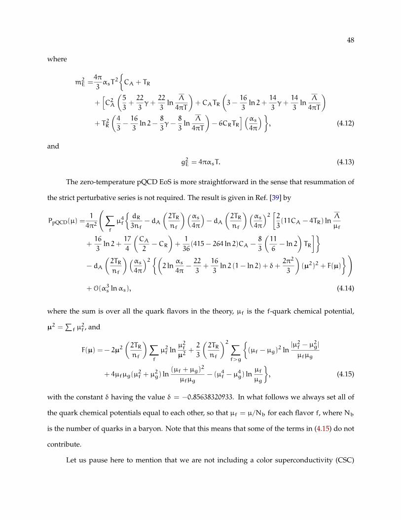
48
where
m2E =4π
3αsT
2
CA + TR
+[C2A
(5
3+22
3γ+
22
3ln
Λ
4πT
)+ CATR
(3−
16
3ln 2+
14
3γ+
14
3ln
Λ
4πT
)+ T2R
(4
3−16
3ln 2−
8
3γ−
8
3ln
Λ
4πT
)− 6CRTR
] (αs4π
), (4.12)
and
g2E = 4παsT. (4.13)
The zero-temperature pQCD EoS is more straightforward in the sense that resummation of
the strict perturbative series is not required. The result is given in Ref. [39] by
PpQCD(µ) =1
4π2
(∑f
µ4f
dR3nf
− dA
(2TRnf
)(αs4π
)− dA
(2TRnf
)(αs4π
)2 [23(11CA − 4TR) ln
Λ
µf
+16
3ln 2+
17
4
(CA2
− CR
)+1
36(415− 264 ln 2)CA −
8
3
(11
6− ln 2
)TR
]− dA
(2TRnf
)(αs4π
)2(2 ln
αs
4π−22
3+16
3ln 2 (1− ln 2) + δ+
2π2
3
)(µ2)2 + F(µ)
)
+ O(α3s lnαs), (4.14)
where the sum is over all the quark flavors in the theory, µf is the f-quark chemical potential,
µ2 =∑f µ2f , and
F(µ) = − 2µ2(2TRnf
)∑f
µ2f lnµ2fµ2
+2
3
(2TRnf
)2∑f>g
(µf − µg)
2 ln|µ2f − µ
2g|
µfµg
+ 4µfµg(µ2f + µ
2g) ln
(µf + µg)2
µfµg− (µ4f − µ
4g) ln
µfµg
, (4.15)
with the constant δ having the value δ = −0.85638320933. In what follows we always set all of
the quark chemical potentials equal to each other, so that µf = µ/Nb for each flavor f, where Nb
is the number of quarks in a baryon. Note that this means that some of the terms in (4.15) do not
contribute.
Let us pause here to mention that we are not including a color superconductivity (CSC)
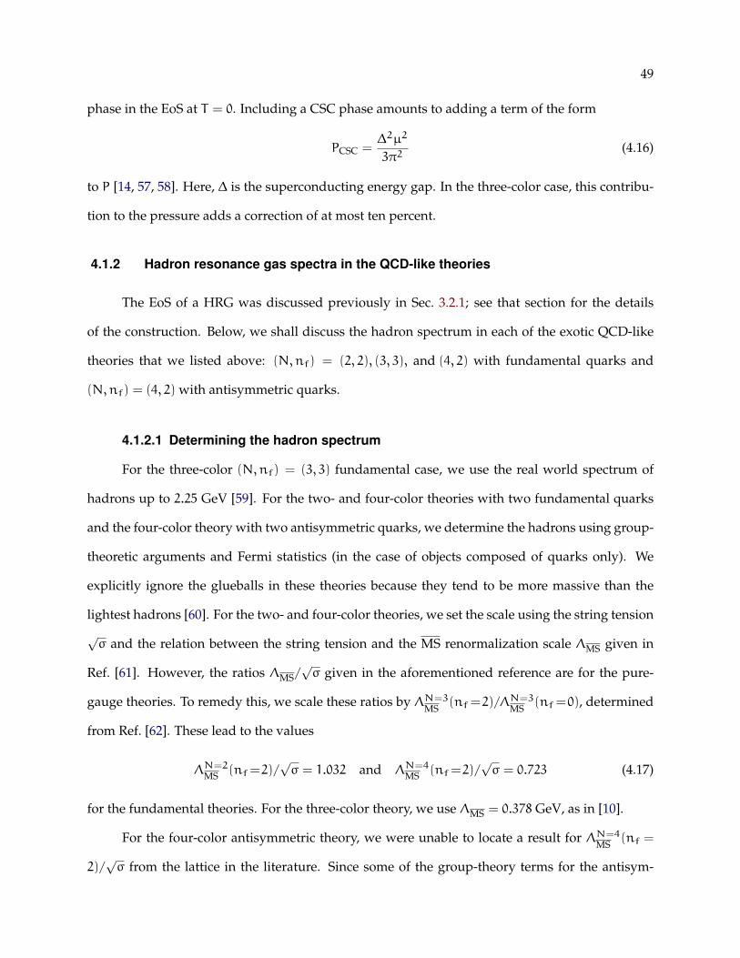
49
phase in the EoS at T = 0. Including a CSC phase amounts to adding a term of the form
PCSC =∆2µ2
3π2(4.16)
to P [14, 57, 58]. Here, ∆ is the superconducting energy gap. In the three-color case, this contribu-
tion to the pressure adds a correction of at most ten percent.
4.1.2 Hadron resonance gas spectra in the QCD-like theories
The EoS of a HRG was discussed previously in Sec. 3.2.1; see that section for the details
of the construction. Below, we shall discuss the hadron spectrum in each of the exotic QCD-like
theories that we listed above: (N,nf) = (2, 2), (3, 3), and (4, 2) with fundamental quarks and
(N,nf) = (4, 2) with antisymmetric quarks.
4.1.2.1 Determining the hadron spectrum
For the three-color (N,nf) = (3, 3) fundamental case, we use the real world spectrum of
hadrons up to 2.25 GeV [59]. For the two- and four-color theories with two fundamental quarks
and the four-color theory with two antisymmetric quarks, we determine the hadrons using group-
theoretic arguments and Fermi statistics (in the case of objects composed of quarks only). We
explicitly ignore the glueballs in these theories because they tend to be more massive than the
lightest hadrons [60]. For the two- and four-color theories, we set the scale using the string tension√σ and the relation between the string tension and the MS renormalization scale ΛMS given in
Ref. [61]. However, the ratios ΛMS/√σ given in the aforementioned reference are for the pure-
gauge theories. To remedy this, we scale these ratios by ΛN=3MS
(nf=2)/ΛN=3MS
(nf=0), determined
from Ref. [62]. These lead to the values
ΛN=2MS (nf=2)/
√σ = 1.032 and ΛN=4
MS (nf=2)/√σ = 0.723 (4.17)
for the fundamental theories. For the three-color theory, we use ΛMS = 0.378 GeV, as in [10].
For the four-color antisymmetric theory, we were unable to locate a result for ΛN=4MS
(nf =
2)/√σ from the lattice in the literature. Since some of the group-theory terms for the antisym-

50
metric theory scale more strongly with the number of colors than the corresponding terms in the
fundamental theory, it seems reasonable to expect that ΛMS will scale differently with the number
of quark flavors in the antisymmetric theory than in the fundamental theory. Moreover, it would
be most accurate to view ΛMS/√σ as a free parameter in the HRG+pQCD scheme that must be
determined independently from the lattice. In light of these considerations, we have decided to
use both the pure-glue value [61]
ΛN=4MS /
√σ = 0.527, (4.18)
and the previously-given value of ΛN=4MS
(nf = 2)/√σ that we use for the four-color fundamental
theory for the four-color antisymmetric theory, with the expectation that the true value will lie
somewhere near this range.
For both the two- and four-color cases, the mesons are taken to be the analogues of the
flavorless mesons that exist in the real world (up to a mass of about 2 GeV) whose masses are
written in multiples of the string tension σSU(3) = (420 MeV)2. In the two-color case, we mainly
use the analogues of the real-world mesons, substituting the two-color masses calculated by Bali
et al. [63] when available. (We also note here that the µ-dependence of the two-color spectrum
has been studied numerically in Ref. [64] and analytically in Ref. [45], though we do not need this
µ-dependence for our HRG+pQCD scheme.)
We now discuss in some detail how the non-meson objects in these three cases are deter-
mined. For convenience and as a summary of these sections, we list tables for all of the particles
that we have included in the SU(2) and SU(4) cases in Appendix A.
Two-color case
In two-color QCD, the baryons are composed of two quarks with the added simplicity that
the masses are degenerate with the corresponding mesons made from the same quarks [65]. Thus,
the mass spectrum of the baryons is the same as the mass spectrum of mesons. However, there
are fewer baryons than mesons, for there is an additional constraint imposed by Fermi statistics in
the case of the baryons. Since we may view the two massless quarks as part of an isospin doublet,

51
one sees that exchanging the two internal quarks in a baryon causes the wave function to become
multiplied by
(−1)1+L+S+I. (4.19)
In this equation, L is the angular momentum quantum number, S is the spin, and I is the isospin,
with the additional 1 due to the fact that the quarks are in an antisymmetric color singlet. We thus
see that for even L the spin and isospin must be equal (S = 0 implies I = 0 and S = 1 implies I = 1),
and for odd L they must be the opposite in order to have a totally antisymmetric wave function.
(Even though the composite baryon is itself a boson in two-color QCD, it is still a multi-particle
state of fundamental fermions.) This information is enough to determine the set of hadrons in the
HRG pressure (3.93).
Four-color fundamental case
Baryons in four-color QCD with fundamental fermions consist of four quarks. In this case,
to determine the massesMwe use the large-N expansion
M(J) = NA+J(J+ 1)
NB, (4.20)
where J is the total angular momentum of the baryon, and A, B are constants independent of
N [66, 67]. As pointed out by DeGrand [68] and demonstrated by Appelquist et al. [69], a term
independent of N could be used for better agreement. However, we have no way to set the value
of such a term and thus do not include it.
We find the possible values of J beginning with the ground-state baryons of zero orbital
angular momentum. Since we still have a isospin doublet of massless, spin-one-half quarks, we
only need the group-theory expression
2⊗ 2⊗ 2⊗ 2 = 5S ⊕ 3M ⊕ 3M ⊕ 3M ⊕ 1A ⊕ 1A, (4.21)
where the 5S state is fully symmetric, the 3M states are are symmetric in three of the four quarks
and antisymmetric in the other, and the 1A states are pairwise antisymmetric. Since, again, the
quarks are in an antisymmetric color singlet, it must be the case that they are in a symmetric com-

52
bination of spin and flavor. This means that there is a spin-2 quintet, a spin-1 triplet, and a spin-0
singlet of ground-state baryons.
We may also determine the first excited states in this simple manner by realizing that for
this four-body problem there are three relevant orbital-angular-momentum quantum numbers
and the first excited state corresponds to when exactly one of them is one. In order to still be in a
completely antisymmetric state, either the spin or the flavor state must now be in one of the 3M
states while the other must be in a 5S state. This means that there are a quintet of particles with
S = 1 and a triplet of particles with S = 2. Combining these with an orbital angular momentum
L = 1 yields three baryonic quintets with J = 0, 1, 2 and three baryonic triplets with J = 1, 2, 3. We
did not determine the baryons for any higher excited states.
Four-color antisymmetric case
The hadron spectrum in the four-color theory with two antisymmetric quarks consists of
two-quark objects: mesons and diquarks; four-quark objects: tetraquarks, di-mesons, and diquark-
mesons; and six-quark baryons [70, 71, 72]. Since the antisymmetric representation is real, the
arguments of Ref. [65] carry through here and one may conclude that all two-quark objects with
the same quark content have degenerate masses and that the same holds for the four-quark ob-
jects. In addition, the four-quark objects have a mass equal to the sum of their constituent two-
quark-object masses [70]. Because of this mass degeneracy, we need not determine how all of the
four-quark-object degrees of freedom break up into spin and isospin multiplets; rather, we may
simply combine the two-quark-object degrees of freedom in every possible way. One major differ-
ence from the two-color case, however, is that in the four-color theory with antisymmetric quarks
the color-singlet state for diquarks is symmetric. This means that the spin-isospin locking in this
theory is the opposite of the locking in the two-color theory. That is, for odd L the spin and isospin
must be equal (S = 0 implies I = 0 and S = 1 implies I = 1), and for even L they must be opposite.
As for the six-quark baryons, we again use the large-N expression (4.20), but with N replaced by
Nb = 6, the number of quarks in the baryon. We include only the ground-state baryons, where

53
isospin and spin are locked as I = J = 3, 2, 1, and 0 [70].
4.1.2.2 Chiral symmetry breaking and the Nambu–Goldstone bosons
The lowest-mass particles in all of the aforementioned theories are precisely zero at zero
quark mass. This can be understood in terms of the pattern of chiral symmetry breaking in these
theories [73]. Consider an SU(N) gauge theory with nf massless fermions. For fermions in a com-
plex representation (such as in the cases N > 3 with fundamental fermions—discussed above in
Sec. 3.2.2), the Lagrangian density possesses the symmetry U(nf)L ⊗ U(nf)R, corresponding to
the separate left- and right-handed flavor symmetries; and for real representations (such as anyN
with adjoint fermions orN = 4with antisymmetric fermions) or pseudoreal representations (such
as in N = 2 with fundamental fermions), the Lagrangian density possesses the larger symmetry
U(2nf). In all of these cases, the axial U(1)A symmetry is broken by an anomaly, and the re-
maining symmetries are spontaneously broken in the following ways. For fermions in a complex
representation:
SU(nf)L ⊗ SU(nf)R → SU(nf)V ; (4.22)
for fermions in a real representation:
SU(2nf) → O(2nf); (4.23)
and for fermions in a pseudoreal representation:
SU(2nf) → Sp(2nf). (4.24)
(See Refs. [73, 45] for more details.) The generators of the broken symmetries become massless
Nambu–Goldstone bosons. Since SU(nf) has n2f−1 generators, O(nf) has nf(nf−1)/2 generators,
and Sp(nf) has nf(nf + 1)/2 generators, we see that in the three-color, three fundamental-quark
case there will be 8Nambu–Goldstone bosons (a meson octet); in the four-color, two fundamental-
quark case there will be 3 Nambu–Goldstone bosons (a meson triplet); in the four-color, two
antisymmetric-quark case there will be 9 Nambu–Goldstone bosons (a triplet each of mesons,

54
diquarks, and antidiquarks); and in the two-color, two fundamental-quark case there will be 5
Nambu–Goldstone bosons (a triplet of mesons, a diquark, and an antidiquark).
In addition, recall that if the quarks in these theories are not precisely massless, then the
massless Nambu–Goldstone bosons will become instead small-mass, pseudo-Nambu–Goldstone
bosons. In the spectra, we are free to vary the mass of these lightest particles to see what effects
this will have on the EoS of the theories. This is especially interesting for lattice practitioners. We
discuss this further in Sec. 4.1.4.
4.1.3 Matching the pQCD and HRG equations of state
To match the two asymptotic EoSs, we employ the same technique on the T -axis as on the
µ-axis. As such, let us introduce the symbol F to stand for either T or µ so that we may discuss the
matching in full generality.
To perform the matching, we take the simpler approach discussed at the beginning of this
chapter: we use each EoS until they intersect, and we assume that at the phase-transition point the
pressures of the two phases are equal. We use the thermodynamic constraints that the pressure of
a system must increase with F
P(F+ ∆F) > P(F), (4.25)
and that above a phase-transition point, the physical phase is the one with the higher pressure.
We also add a bag constant B to the pQCD pressure so that
PpQCD(F) = P0pQCD(F) + B, (4.26)
where P0pQCD is given by either (4.6)-(4.11) or (4.14). In the plots that follow, we solve the following
set of two equations with two unknowns (for a given Λ):
PHRG(F0) = PpQCD(F0, B0), (4.27)
dPHRG(F)
dF
∣∣∣∣F=F0
=∂PpQCD(F, B0)
∂F
∣∣∣∣F=F0
. (4.28)
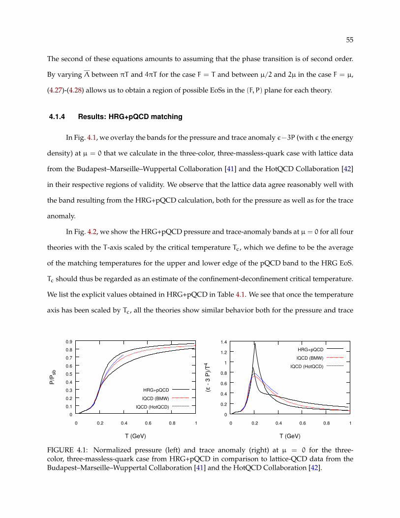
55
The second of these equations amounts to assuming that the phase transition is of second order.
By varying Λ between πT and 4πT for the case F = T and between µ/2 and 2µ in the case F = µ,
(4.27)-(4.28) allows us to obtain a region of possible EoSs in the (F, P) plane for each theory.
4.1.4 Results: HRG+pQCD matching
In Fig. 4.1, we overlay the bands for the pressure and trace anomaly ε−3P (with ε the energy
density) at µ = 0 that we calculate in the three-color, three-massless-quark case with lattice data
from the Budapest–Marseille–Wuppertal Collaboration [41] and the HotQCD Collaboration [42]
in their respective regions of validity. We observe that the lattice data agree reasonably well with
the band resulting from the HRG+pQCD calculation, both for the pressure as well as for the trace
anomaly.
In Fig. 4.2, we show the HRG+pQCD pressure and trace-anomaly bands at µ = 0 for all four
theories with the T -axis scaled by the critical temperature Tc, which we define to be the average
of the matching temperatures for the upper and lower edge of the pQCD band to the HRG EoS.
Tc should thus be regarded as an estimate of the confinement-deconfinement critical temperature.
We list the explicit values obtained in HRG+pQCD in Table 4.1. We see that once the temperature
axis has been scaled by Tc, all the theories show similar behavior both for the pressure and trace
0
0.1
0.2
0.3
0.4
0.5
0.6
0.7
0.8
0.9
0 0.2 0.4 0.6 0.8 1
P/P
sb
T (GeV)
HRG+pQCD
lQCD (BMW)
lQCD (HotQCD)
0
0.2
0.4
0.6
0.8
1
1.2
1.4
0 0.2 0.4 0.6 0.8 1
(ε -
3 P
)/T
4
T (GeV)
HRG+pQCD
lQCD (BMW)
lQCD (HotQCD)
FIGURE 4.1: Normalized pressure (left) and trace anomaly (right) at µ = 0 for the three-color, three-massless-quark case from HRG+pQCD in comparison to lattice-QCD data from theBudapest–Marseille–Wuppertal Collaboration [41] and the HotQCD Collaboration [42].

56
0
0.1
0.2
0.3
0.4
0.5
0.6
0.7
0.8
0.9
0 0.5 1 1.5 2 2.5 3 3.5 4 4.5 5
P/P
sb
T/Tc
Two-Color Fundamental
Three-Color Fundamental
Four-Color Fundamental
Four-Color Antisymmetric
0
0.2
0.4
0.6
0.8
1
1.2
1.4
0 0.5 1 1.5 2 2.5 3 3.5 4 4.5 5
(ε -
3P
)/P
sb
T/Tc
Two-Color Fundamental
Three-Color Fundamental
Four-Color Fundamental
Four-Color Antisymmetric
FIGURE 4.2: Normalized pressure (left) and trace anomaly (right) at µ = 0 for the two-color,three-color, four-color fundamental, and four-color antisymmetric theories in HRG+pQCD. Notethat the T -axis has been scaled by the critical temperature (see main text).
anomaly, a phenomenon that is well-known from pure-gauge theories [74].
The differences at low temperatures are due to the different numbers of Nambu–Goldstone
bosons in the two-color and four-color theories with zero quark mass (see Sec. 4.1.2.2 or Ap-
pendix A) and the fact that in the real world there are only pseudo-Nambu–Goldstone bosons.
We verified this by increasing the mass of the lightest (now pseudo-) Nambu–Goldstone bosons,
which qualitatively changed the shape of the pressure curves until they matched that of the real-
world, three-color theory. In Fig. 4.3, we show the pressure and trace-anomaly bands at T = 0 for
all four theories with the µ-axis scaled by the critical chemical potential µc, again, defined to be the
average of the matching chemical potential of the upper and lower edge of the pQCD band to the
HRG EoS. The value of µc should be regarded as an estimate for the confinement-deconfinement
transition, whereas the critical chemical potential for the onset transition would be given by the
smallest value of mi/ri, to use the notation of Sec. 4.1.2. In the fundamental theories, this value
of mi/ri corresponds to the lightest baryon mass. Similar to the µ = 0 case, the µ 6= 0, T = 0
results show similar trends when scaled appropriately. Again, the different behaviors at low µ/µc
are due to the fact that there are Nambu–Goldstone bosons composed solely of quarks in the two-
color fundamental and four-color antisymmetric theories. Again, this was tested by increasing the
masses of the lightest particles.
The values of Tc/√σ and µc/
√σ for the HRG+pQCD calculations are given in Tab. 4.1.

57
0
0.1
0.2
0.3
0.4
0.5
0.6
0.7
0.8
0.9
0 0.5 1 1.5 2 2.5 3 3.5 4 4.5 5
P/P
fd
µ/µc
Two-Color Fundamental
Three-Color Fundamental
Four-Color Fundamental
Four-Color Antisymmetric
0
0.5
1
1.5
2
2.5
3
3.5
0 0.5 1 1.5 2 2.5 3 3.5 4 4.5 5
(ε -
3P
)/P
fd
µ/µc
Two-Color Fundamental
Three-Color Fundamental
Four-Color Fundamental
Four-Color Antisymmetric
FIGURE 4.3: Normalized pressure (left) and trace anomaly (right) at T = 0 for the two-color,three-color, four-color fundamental, and the four-color antisymmetric theories in HRG+pQCD.Note that the µ-axis has been scaled by the critical chemical potential (see main text).
While the results suggests that the Tc values for the different theories are within 20 percent of each
other, the extracted µc values span a much broader range.
We wish to remind the reader here that, in the T = 0 case, we have not included the CSC
phase in the high-µ EoS, which will introduce a correction to the pressure on the ten-percent level
(see the discussion near Eq. (4.16)). We also note that a ten-percent change in the plots of the bulk
thermodynamic properties will not affect them in a noticeable way, for the error bands are already
at least of this order.
We stress that in the four-color antisymmetric case with ΛMS/√σ = 0.723, we were unable
to carry out the matching procedure at µ = 0 in the chiral limit. We found that in this case, the
HRG pressure rose too sharply and never intersected the pQCD pressure-band. Thus, we have
only plotted the ΛMS/√σ = 0.527 results for the four-color antisymmetric theory in the figures.
Group, Representation, nf Tc/√σ µc/
√σ
SU(2), fundamental, 2 0.400 3.24SU(3), fundamental, 3 0.47 2.382SU(4), fundamental, 2 0.44 2.853
SU(4), antisymmetric, 2 (ΛMS/√σ = 0.527) 0.29 5.09
SU(4), antisymmetric, 2 (ΛMS/√σ = 0.723) no matching 5.0
TABLE 4.1: The ratios Tc/√σ and µc/
√σ for the theories analyzed in this section. Errors are given
by the number of significant figures.

58
0
0.1
0.2
0.3
0.4
0.5
0 0.1 0.2 0.3 0.4 0.5 0.6 0.7 0.8
Tc / √σ
Mpion / √σ
FIGURE 4.4: Deconfinement-transition temperature Tc as a function of pion mass for the four-color, antisymmetric theory in the µ = 0, ΛMS/
√σ = 0.723 case. The straight line is a fit to the
results where matching could be performed, and defines the extrapolation to the chiral limit (seemain text).
We feel this is justified for a few reasons. First of all, the values of µc are equal within uncertainties
for the two different values of ΛMS/√σ. Secondly, in the case where ΛMS/
√σ = 0.723, we were
able to carry out the HRG+pQCD matching procedure when we increased the mass of the lightest
bosons (the pion mass). By varying the pion mass, we were able to extrapolate to the chiral limit,
obtaining a value of µc/√σ = 0.3, which agrees with the value found for ΛMS/
√σ = 0.527 (see
Tab. 4.1). In light of this agreement, and in light of how the four-color antisymmetric theory was
the only theory where the matching was strained, we conjecture that the true value of ΛMS/√σ in
this case is closer to the pure-glue value than it is in the real-world, three-color case. We point out
that this prediction could be tested in future lattice-gauge-theory calculations.
Finally, we have calculated the speed of sound cs at T = 0 in all four QCD-like theories us-
ing the HRG+pQCD scheme, shown in Fig. 4.5. We note that in some cases, cs exceeds the speed
of light, and thus these particular matching results from HRG+pQCD should be considered un-
physical (a standard constraint when using cold-nuclear-matter EoSs). Nevertheless, our results
indicate that it is generally possible to obtain physical EoSs wherein c2s > 1/3 for all fundamental
QCD-like theories. This finding could be of interest because restricting c2s < 1/3 has previously
been noted to be in tension with astrophysical observations [75]. Again, we point out that this is a
property which could be tested in future lattice-gauge-theory calculations.
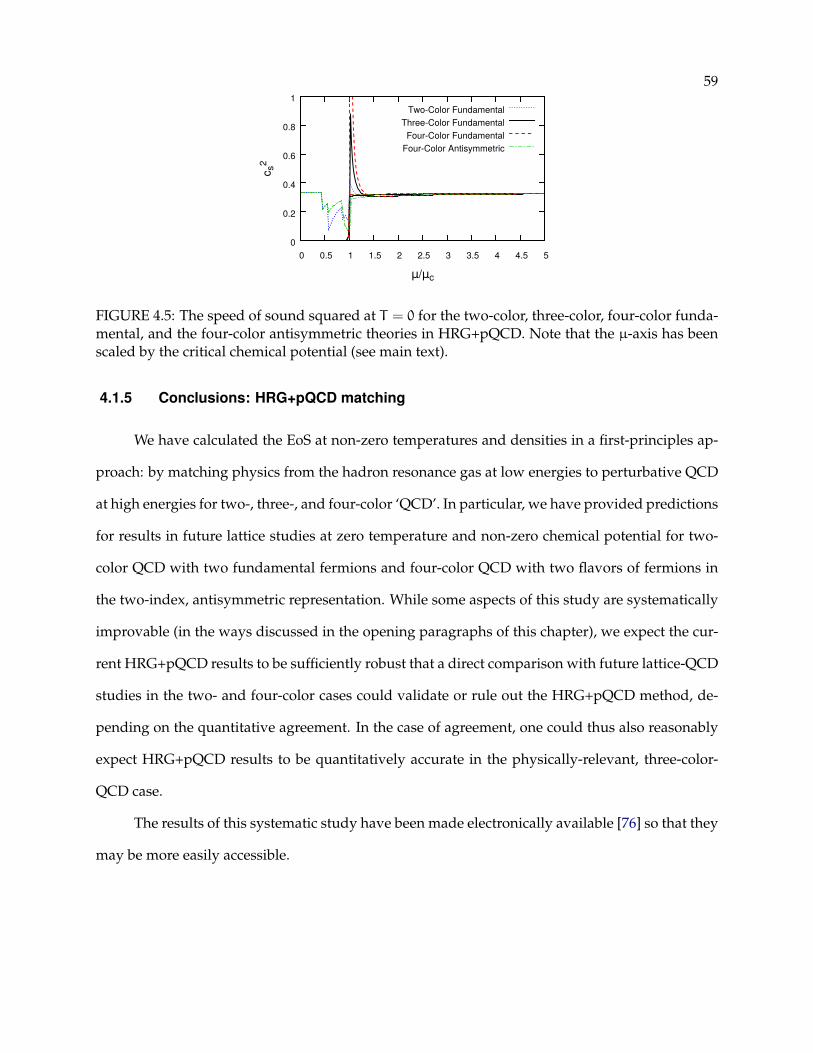
59
0
0.2
0.4
0.6
0.8
1
0 0.5 1 1.5 2 2.5 3 3.5 4 4.5 5
cs2
µ/µc
Two-Color Fundamental
Three-Color Fundamental
Four-Color Fundamental
Four-Color Antisymmetric
FIGURE 4.5: The speed of sound squared at T = 0 for the two-color, three-color, four-color funda-mental, and the four-color antisymmetric theories in HRG+pQCD. Note that the µ-axis has beenscaled by the critical chemical potential (see main text).
4.1.5 Conclusions: HRG+pQCD matching
We have calculated the EoS at non-zero temperatures and densities in a first-principles ap-
proach: by matching physics from the hadron resonance gas at low energies to perturbative QCD
at high energies for two-, three-, and four-color ‘QCD’. In particular, we have provided predictions
for results in future lattice studies at zero temperature and non-zero chemical potential for two-
color QCD with two fundamental fermions and four-color QCD with two flavors of fermions in
the two-index, antisymmetric representation. While some aspects of this study are systematically
improvable (in the ways discussed in the opening paragraphs of this chapter), we expect the cur-
rent HRG+pQCD results to be sufficiently robust that a direct comparison with future lattice-QCD
studies in the two- and four-color cases could validate or rule out the HRG+pQCD method, de-
pending on the quantitative agreement. In the case of agreement, one could thus also reasonably
expect HRG+pQCD results to be quantitatively accurate in the physically-relevant, three-color-
QCD case.
The results of this systematic study have been made electronically available [76] so that they
may be more easily accessible.

60
4.2 Kurkela et al. [1] matching: ChEFT to pQCD
The second topic that we address in this chapter is the current state-of-the-art matched EoS
of Kurkela et al. [1], which demonstrates the more sophisticated matching approach discussed in
the introductory paragraphs of this chapter. In the papers in Refs. [1, 11], the authors conducted a
careful matching procedure to constrain the QCD EoS between the ChEFT and pQCD limits. The
authors only assumed the validity of the perturbative EoSs up to a point, and between these two
extremes they approximated the QCD EoS by two or more (though see below) polytropic EoSs,
i.e., EoSs of the form
P(n) = κinγi , (4.29)
where n is the density, κi and γi are constants, and i labels the different polytropes. The expo-
nent γi is referred to as the polytropic index. The matching to the ChEFT and pQCD EoSs was
performed at n = 1.1ns and µ = 2.6 GeV, respectively, where the relative uncertainties for each
perturbative EoS reach ±24% [77, 10]. Here, ns ≈ 0.16/fm3 is the nuclear saturation density.
Below n = 1.1ns, the authors used the state-of-the-art ChEFT EoS of Tews et al. [77], and above
µ = 2.6 GeV, the authors used the state-of-the-art pQCD EoS from Ref. [10] in the compact form
presented in Ref. [78].
Between these two controlled regimes, the authors of Ref. [1] used either two or three poly-
topes of the form (4.29) both with and without latent heat (i.e., a first-order phase transition) at the
matching points. The authors eventually concluded that the addition of latent heat was actually
more restrictive on the matching, and, in addition, a third polytrope only minimally increased the
range of allowed EoSs (see Fig. 4.6, taken from their paper). Thus, in the rest of our descriptions
here, we will outline the procedure used in Ref. [1] to match two intermediate polytropes.
To match the two polytropic EoSs, the authors chose a random intermediate matching value
µc and a matching point in the pQCD band (obtained by varying the renormalization scale Λ
about√(2πT)2 + (µ)2 by a factor of two in both directions, as is customary) and attempted to
solve for the polytropic indices γi that would provide a matched EoS for those random values. If
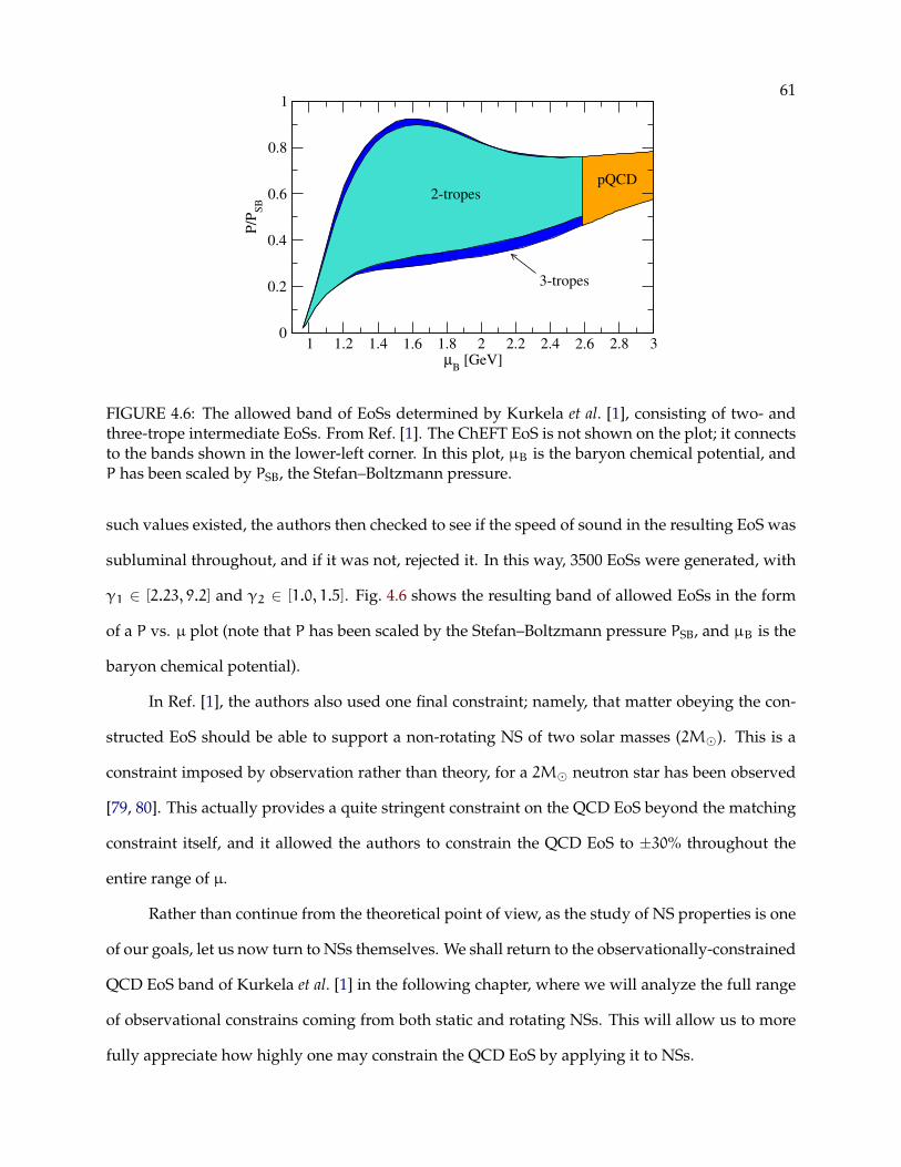
61
1 1.2 1.4 1.6 1.8 2 2.2 2.4 2.6 2.8 3µ
B [GeV]
0
0.2
0.4
0.6
0.8
1
P/P
SB
2-tropes
3-tropes
pQCD
FIGURE 4.6: The allowed band of EoSs determined by Kurkela et al. [1], consisting of two- andthree-trope intermediate EoSs. From Ref. [1]. The ChEFT EoS is not shown on the plot; it connectsto the bands shown in the lower-left corner. In this plot, µB is the baryon chemical potential, andP has been scaled by PSB, the Stefan–Boltzmann pressure.
such values existed, the authors then checked to see if the speed of sound in the resulting EoS was
subluminal throughout, and if it was not, rejected it. In this way, 3500 EoSs were generated, with
γ1 ∈ [2.23, 9.2] and γ2 ∈ [1.0, 1.5]. Fig. 4.6 shows the resulting band of allowed EoSs in the form
of a P vs. µ plot (note that P has been scaled by the Stefan–Boltzmann pressure PSB, and µB is the
baryon chemical potential).
In Ref. [1], the authors also used one final constraint; namely, that matter obeying the con-
structed EoS should be able to support a non-rotating NS of two solar masses (2M). This is a
constraint imposed by observation rather than theory, for a 2M neutron star has been observed
[79, 80]. This actually provides a quite stringent constraint on the QCD EoS beyond the matching
constraint itself, and it allowed the authors to constrain the QCD EoS to ±30% throughout the
entire range of µ.
Rather than continue from the theoretical point of view, as the study of NS properties is one
of our goals, let us now turn to NSs themselves. We shall return to the observationally-constrained
QCD EoS band of Kurkela et al. [1] in the following chapter, where we will analyze the full range
of observational constrains coming from both static and rotating NSs. This will allow us to more
fully appreciate how highly one may constrain the QCD EoS by applying it to NSs.

CHAPTER 5
NEUTRON STARS AND APPLICATIONS
Neutron stars (NSs) are one of the most extreme physical systems in the cosmos. Within a
sphere of radius ∼10 km lies over 1M of matter. In the outer layers of NSs, controlled techniques
such as ChEFT [77] or quantum Monte Carlo [81] are applicable and can yield insights into both
the static properties of the bulk matter (such as the equation of state or EoS) and some transport
properties. Currently, these low-density calculations are valid up to about 1.1 times the nuclear
saturation density ns ≈ 0.16/fm3, corresponding to a baryon chemical potential of about µ ≈
0.97 GeV [77]. Deep in the core, however, such controlled, direct theoretical calculations are not
possible. This is because the densities and chemical potentials at the center of the star, though
extreme, are not large enough to fall into the range accessible by pQCD. In the state-of-the-art
pQCD calculations at zero temperature in Ref. [10], the errors associated with varying the mass
scale reach 30% at around µ = 2.6 GeV. The value of µ in the cores of NSs lies within a subset of
this 0.97− 2.6 GeV range.
The problem of the interiors of NSs is thus currently a non-perturbative one. However,
as discussed in Chap. 4, one can hope to reach the intermediate values of µ by matching the
low-density EoS from a low-energy effective theory to the pQCD results in a thermodynamically
consistent way to investigate the makeup of NSs. As also discussed in that chapter, this has been
carried out in the work of Kurkela et al. [1] and Fraga et al. [11], who, in addition, incorporated

63
the 2M constraint from Refs. [79, 80]. (See also Ref. [82], in which the authors use only ChEFT
and the 2M constraint to extend the low-energy EoS.) In these works, the authors used their
matched EoSs to analyze non-rotating NSs only. It is known [83, 84] that slowly-rotating NSs can
be approximated as non-rotating for frequencies of rotation less than about f ≈ 200 Hz. Beyond
this, however, one must use numerical codes to analyze the structure of the stars. Such a numerical
approach has been recently used by Cipolletta et al. [84] and Haensel et al. [85] in the context of
phenomenological EoSs, and one of the purposes of this chapter is to extend these analyses to
include EoSs that are more fully constrained by first-principles physics.
Broadly speaking, the purpose of this chapter is to investigate the structure of NSs at fre-
quencies from zero all the way up to the mass-shedding limit using the constraints on the QCD
EoS determined in Refs. [1, 11]. We are particularly interested in constraining NS properties that
are relevant observationally. In Sec. 5.1, we quickly review the general procedure for constraining
global NS structure within the framework of general relativity (GR). Then, in Sec. 5.2, we con-
sider applications of the QCD EoS band of Kurkela et al. [1]. In this section, we first discuss the
work done in Ref. [1] to incorporate the 2M constraint into the authors’ matching procedure
and highlight their conclusions about observable NS properties. We follow this discussion with
original work that extends these results to rotating NSs. We investigate the maximum allowed
NS masses, as well as the allowed regions for mass–radius curves, mass–frequency curves, and
radius–frequency curves for a typical 1.4M star. In addition, we investigate the allowed values
of the moment of inertia of the double pulsar PSR J0737-3039A [86, 87] and study how this is cor-
related with the radius. In this way, we aim to provide a strong direct link between astronomical
observations and the allowed QCD EoSs coming from current state-of-the-art pQCD and ChEFT
calculations.
This chapter draws heavily from work that will soon be published in Ref. [88].

64
5.1 The QCD EoS and the structure of NSs: overview
To determine the global structure of a NS in GR, one often starts with symmetry assump-
tions. The two simplest assumptions are that the star is non-rotating, or rotating uniformly. Let us
begin with the former case.
A non-rotating, spherically-symmetric object in GR can be described by the metric [89]
ds2 = e2α(r) dt2 − e2β(r) dr2 − r2(dθ2 + sin2 θdφ2
). (5.1)
Here, α and β are arbitrary functions of r. To compute the structure of a NS, one must solve
Einstein’s Equations,
Rµν −1
2gµνR = 8πGTµν, (5.2)
inside the star, where we assume that the matter in the star is a perfect fluid with
Tµν = (ε+ P)uµuν − Pgµν. (5.3)
In these equations, G is Newton’s gravitational constant, uµ is the four-velocity of a fluid element,
and, as before, ε is the energy density and P is the pressure. Using algebra, the equations (5.1)-(5.3)
can be reduced to the following two equations, called the Tolman–Oppenheimer–Volkoff or TOV
equations [89]:
dPdr
= −G(ε+ P)
[m(r) + 4πr3P
]r[r− 2Gm(r)
] , (5.4)
dmdr
= 4πr2ε. (5.5)
Note that these are simply the equations describing hydrostatic equilibrium for a static, spherically-
symmetric fluid. To solve for the structure of a non-rotating NS, one must prescribe an EoS (i.e.,
P(ε)). With this specified, one may construct a star by specifying a central energy density ε∗ and
then solving the TOV equations outward from the center until the radius R such that ε(R) = 0; this
is the stellar surface.
For a uniformly-rotating star, the procedure is in principle the same, though the equations
are more complicated. The metric of a stationary, axisymmetric space-time (i.e., one describing a

65
uniformly-rotating, axisymmetric star with angular velocity Ω as judged by an observer at infin-
ity) is given by [90, 91, 92]
ds2 = e2ν dt2 − e2α(dr2 + r2 dθ2
)− e2βr2 sin2 θ
(dφ−ωdt
)2, (5.6)
where ν, ω, α, and β are functions of r and θ. In this case, one must again solve Einstein’s Equa-
tions (5.2) with the assumption (5.3) for Tµν. This leads to the following equation for hydrosta-
tionary equilibrium (as opposed to hydrostatic equilibrium when there was no motion at all) [93,
92]:1
ε+ P∇P +∇ν−
1
2∇ ln(1−w2) = 0, (5.7)
where here, w is the proper velocity of a fluid element with respect to a local zero-angular-
momentum observer:
w = r sin θeβ−ν(Ω−ω). (5.8)
Note that in this rotational case, the hydrostationary-equilibrium equation is not decoupled from
the Einstein equations.
The coupled system of (5.8) and Einstein’s Equations (5.2) can be solved numerically with
the use of the publicly-available RNS code of Ref. [94]. This code takes as input an EoS in the
form P(ε) and two parameters: a central energy density ε∗ and the ratio of the polar coordinate
radius to the equatorial coordinate radius r∗. Other inputs can be used as well (see Sec. 5.2.2,
where we use this code in combination with the QCD EoS of Kurkela et al. [1]), but internally each
NS that is constructed is specified by the parameters ε∗ and r∗. From this input, the code can
calculate various global properties of the star, including the total (or gravitational) mass M, the
circumferential equatorial radius Re, the frequency of rotation f, and the moment of inertia I.
5.2 Global properties of NSs with QCD EoSs
In this section, we discuss applications of the QCD EoS band of Refs. [1, 11] to NS. These
applications take two complementary forms. First, the QCD EoS band can be used to constrain
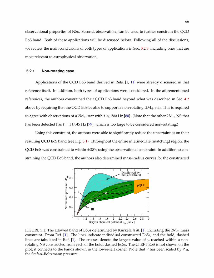
66
observational properties of NSs. Second, observations can be used to further constrain the QCD
EoS band. Both of these applications will be discussed below. Following all of the discussions,
we review the main conclusions of both types of applications in Sec. 5.2.3, including ones that are
most relevant to astrophysical observation.
5.2.1 Non-rotating case
Applications of the QCD EoS band derived in Refs. [1, 11] were already discussed in that
reference itself. In addition, both types of applications were considered. In the aforementioned
references, the authors constrained their QCD EoS band beyond what was described in Sec. 4.2
above by requiring that the QCD EoS be able to support a non-rotating, 2M star. This is required
to agree with observations of a 2M star with f 200 Hz [80]. (Note that the other 2M NS that
has been detected has f = 317.45 Hz [79], which is too large to be considered non-rotating.)
Using this constraint, the authors were able to significantly reduce the uncertainties on their
resulting QCD EoS band (see Fig. 5.1). Throughout the entire intermediate (matching) region, the
QCD EoS was constrained to within ±30% using the observational constraint. In addition to con-
straining the QCD EoS band, the authors also determined mass–radius curves for the constructed
1 1.2 1.4 1.6 1.8 2 2.2 2.4 2.6 2.8 3Baryon chemical potential µ
B [GeV]
0
0.2
0.4
0.6
0.8
1
Norm
aliz
ed p
ress
ure
P/P
SB
Disallowed bymass constraint
I
II
III
pQCD
FIGURE 5.1: The allowed band of EoSs determined by Kurkela et al. [1], including the 2M massconstraint. From Ref. [1]. The lines indicate individual constructed EoSs, and the bold, dashedlines are tabulated in Ref. [1]. The crosses denote the largest value of µ reached within a non-rotating NS constructed from each of the bold, dashed EoSs. The ChEFT EoS is not shown on theplot; it connects to the bands shown in the lower-left corner. Note that P has been scaled by PSB,the Stefan–Boltzmann pressure.

67
EoSs. We do not include their mass–radius plots here, for in the next section we reproduce the
non-rotating region calculated in Ref. [1] as the horizontally-striped area in Fig. 5.2 below. How-
ever, we do note that the authors concluded that any non-rotating NS constructed from their QCD
EoS band must satisfyM < 2.75M (orM < 2.5M for bitropic EoSs), with the radius of a typical
1.4M star falling between 11 and 14.5 km.
Let us now turn to our generalizations of these results to include rotating NSs.
5.2.2 General rotating case
In this section, we discuss generalizations of the work of Ref. [1] to include rotating NSs. We
begin by briefly describing how the RNS code mentioned above in Sec. 5.1 was used to construct
mass–radius curves, mass–frequency curves, radius–frequency curves for a typical 1.4M star,
and moment-of-inertia–radius plots of the double pulsar PSR J0737-3039A. Following this, we
present our results and all of our plots in detail.
Methodology
To conduct our analysis of rotating NSs, we used the publicly available RNS code [94]. In
addition to constructing a single star specified by ε∗ and r∗ (see the discussion in Sec. 5.1 above),
the RNS code can construct sequences of stars as well as accept other stellar properties as input
to construct internal sequences and find stars satisfying those inputs. It can also calculate the
mass-shedding frequency for a given central energy density ε0, which is the fastest rotation rate
possible before the star begins to throw off mass from its equator. This provides an upper bound
on the rotation rate for the central energy density ε0. Rotating stars have both a larger maximum
mass and a larger maximum equatorial radius, and so the mass-shedding limit can be used to
investigate larger, more massive stars than were possible in the non-rotating limit.
The approach used in this investigation was to take the EoSs used in Refs. [1, 11] in the
form P(ε) and feed them into the RNS code to calculate various properties of physical interest. A
comment is in order here. Since in Refs. [1, 11], the authors concluded that adding latent heat was
actually more restrictive on the matching, and, in addition, they found that a third polytrope only

68
minimally increased the range of allowed EoSs, we have also only used the bitropic EoSs without
latent heat in this section.
To construct our data, we first ran the RNS code on the static and mass-shedding sequences.
From this, we could construct the mass–radius curves and one boundary of the allowed mass–
frequency region for NSs. The rest of our numerical data involved either fixed-frequency runs,
fixed-mass runs (or both), or coding a binary search to fill in the gaps where the code was unable
to generate the star. This was necessary in the cases of very small frequencies, as internally the
code always uses r∗ as a parameter instead of f. (This behavior was also noted in Ref. [84].) The
fixed-frequency runs were used to determine the other boundary of the allowed mass–frequency
region, and the fixed-mass runs were used to determine the radius–frequency relations for a typ-
ical, 1.4M NS. Finally, the runs at fixed mass and frequency were used for investigating PSR
J0737-3039A.
Results: Rotating case
We present first our results for mass vs. equatorial radius curves in Fig. 5.2. The non-rotating
region is the same as in Ref. [1], and has a maximum mass of about 2.5M. As seen in the figure,
rotating NSs have a larger radius and a larger maximum mass than non-rotating ones. This can be
thought of as a consequence of centrifugal force: the stars with large central energy densities that
are unstable past the maximum-mass point for non-rotating stars are stabilized (and their central
energy densities are lowered) by the outward centrifugal force in the rotating case. The larger
radius is a consequence of the eccentricity of the star caused by the centrifugal force as well. We
see that the maximum-mass star now has a mass of about 3.25M, and the largest stellar radius is
about 21km.
As one might expect, the boundaries of the non-rotating region and the mass-shedding re-
gions in Fig. 5.2 are formed from the same EoSs; e.g., the EoS that contains the highest-mass
stars in the non-rotating case also contains the highest-mass stars in the mass-shedding case. This
means that any further observational constraints that restrict the left, horizontally-striped region
in Fig. 5.2 will also restrict the right, vertically-striped region in the same way.

69
10 12 14 16 18 20Req [km]
0.5
1.0
1.5
2.0
2.5
3.0
3.5
M [M
sola
r]
FIGURE 5.2: Mass vs. equatorial radius regions for non-rotating stars (horizontal stripes) andmass-shedding stars (vertical stripes). The upper, checkered region is an overlap between thenon-rotating and mass-shedding regions. The lower, solid region is only accessible to non-mass-shedding rotating NSs.
In Fig. 5.3, we show the allowed regions for NSs in the mass–frequency plane. The inner,
solid region is allowed for every EoS, and the outer, checkered band shows where the possible
boundaries are for each EoS. The right boundary of the checkered region is constrained by the
mass-shedding stars: beyond a certain limiting frequency at a given mass, stars become unstable.
The upper boundary of the checkered region consists of the curves Mmax(f), the maximum NS
mass as a function of frequency. We also include a dashed line in Fig. 5.3, which is the boundary
of the mass–frequency region for a sample EoS. This is to illustrate the shape of the boundary for
each EoS. Every EoS is shaped similarly: the top boundary rises towards the sloped, upper-right
edge of the checkered region, comes to a point, and then curves back down. Note that this implies
that the outermost boundary of the checkered region is not formed from a single EoS; in fact, even
the upper edge and lower-right edge of the checkered region are formed by different EoSs.
We also show in Fig. 5.3 data points for NSs with frequencies above 100Hz, taken from
Ref. [85]. A star located in the checkered band would eliminate some of the EoSs (namely, the ones
whose curves in the checkered region are closer to the inner, solid region than the data point of the
star). We see that there is only one star that is pushing into the checkered band: this is B1516+02B.
If the mass of this star were further constrained, it could potentially eliminate a sizeable number of
additional EoSs. Note, however, that f = 125.83Hz for B1516+02B, so this is still within the regime

70
0 500 1000 1500 2000Frequency [Hz]
0.0
0.5
1.0
1.5
2.0
2.5
3.0
3.5
M [M
sola
r]
FIGURE 5.3: The allowed mass–frequency region for all of the possible QCD EoSs. The inner,solid region is allowed for every EoS, and the outer, checkered band shows where the possibleboundaries are for each EoS. The dashed line is the outer boundary of the mass–frequency regionfor a sample EoS. Data points for NSs with f > 100Hz, taken from a table in Ref. [85], are alsoplotted.
where approximating the star as non-rotating is valid. Thus, this constraint is not fundamentally
one of rotation.
From Fig. 5.3, however, we see that for high-f stars, there is a constraint coming from rota-
tion. The clearest example of this is the upper-right corner of the inner, solid region with coordi-
nates (M, f) = (2.06M, 883Hz). This frequency, f = 883Hz, signifies the highest frequency that all
of the EoSs can support. Thus, if a NS is ever found with f > 883Hz, this would eliminate some of
the possible EoSs of Refs. [1, 11]. We note, however, that this is the highest frequency that would
eliminate some EoSs: lower-frequency NSs could also rule out some EoSs if their masses could be
measured and were sufficiently low. For example, PSR J1748-2446ad, currently the fastest rotating
NS known (f = 716Hz) [95], would eliminate some EoSs if its mass is less than about 1M.
For a 1.4M NS, the largest frequency that all EoSs can support is lower, f = 780Hz, as show
in Fig. 5.4. In this figure, we have plotted the equatorial radius as a function of frequency Re(f) for
a typical 1.4M NS for each EoS. This plot serves as a prediction for observational astronomers.
Furthermore, when consistent, reliable data of NS radii are available, a plot of this type could
be overlaid with observational data to further constrain the QCD EoS (similar to Fig. 5.3 above).
One other comment we wish to make here is that this radius–frequency band agrees with the

71
0 200 400 600 800 1000 1200f [Hz]
10
12
14
16
18
20
Re [k
m]
FIGURE 5.4: The region of allowed circumferential equatorial radius vs. frequency curves for a1.4M star.
result of the minimum-χ2, hybrid EoS of Kurkela et al. in Ref. [96]. That result lies directly in
the center of our band in Fig. 5.4. We do note, however, that their mass–frequency boundary
only partially agrees with our band: The boundary of the mass–frequency region coming from
the mass-shedding curve in Ref. [96] lies in the center of our checkered band coming from our
mass-shedding curves, but their upper boundary cuts into our solid band. This is because the
minimum-χ2, hybrid EoS obtained in Ref. [96] does not permit a 2M NS.
The final plot that we have generated from the EoSs is shown in Fig. 5.5. In this figure, we
show the allowed region for the moment of inertia and equatorial radius of PSR J0737-3039A. The
moment of inertia of this star may be measured in a few years [86, 87], and so it is natural to inves-
tigate what the QCD EoSs predicts its value should be. We find that I ∈ [1.2, 1.8]×1045g cm2. Work
of this type has been performed previously assuming phenomenological EoSs, e.g. in Refs. [97,
87, 98]; and, more recently, Raithel et al. [99] have performed an analysis in which an EoS is only
assumed up to ns, and the remaining mass is shifted around to minimize and maximize I for the
star. This allows the authors to plot the largest allowed region in the Re–I plane constrained by
controlled first-principles low-energy physics. Our allowed region in Fig. 5.5 does fall within the
larger-Re, larger-I (i.e., upper-right) portion of the region calculated in the aforementioned work,
and it also falls roughly in the center of the forty EoS data points presented in an earlier figure in
that work.

72
11 12 13 14 15Re [km]
1.0
1.2
1.4
1.6
1.8
2.0
I [×
1045
g c
m2 ]
FIGURE 5.5: The allowed region of moment of inertia vs. circumferential equatorial radius forPSR J0737-3039A.
We also find that all of the “hard” and “soft” EoSs from Refs. [1, 11] fall on the two bound-
aries of our allowed region: the “hard” EoSs form the right boundary and the “soft” ones form
the left boundary. In other words, the “hard” and “soft” EoSs each lie on their own fixed curve.
This is not surprising, since the largest contribution to I comes from the matter at the largest radii
(in the low-density crust region), and there, all the “hard” or “soft” EoSs agree by construction.
Note, however, that since these EoSs form the vertical boundaries of the region, even a relatively
imprecise measurement of the moment of inertia of PSR J0737-3039A (e.g., one with a precision
of 10%) will significantly constrain which EoSs are consistent with the measurement. Since the al-
lowed region spans 0.6 × 1045 g cm2 in I, a 10% measurement will only be consistent with about
0.15/0.6 = 25% of the EoSs.
This percentage is not a physical meaningful result, but we translate it into a statement about
the QCD EoS band in Fig. 5.6. In this figure, we display the QCD EoS band of Kurkela et al. [1],
along with the subset of it that is consistent with I = 1.5× 1045 g cm2 to a precision of 10%, as an
example. We see that such a measurement would shrink the percent errors of the band by up to
50% in some places, especially in the lowest-density regime. Again, this makes sense because it is
the low-density material farthest from the rotation axis that contributes most to I. This reduction
in the QCD EoS band would then, by extension, significantly constrain all of the NS properties
mentioned in this section. This makes a measurement of the moment of inertia of the double

73
100 1000 10000
Energy density [MeV/fm3]
1
10
100
1000
10000
Pre
ssur
e [M
eV/fm
3 ]
pQCDEoS band w/oI constraint
EoS band withI constraint
Neutron matter
FIGURE 5.6: A plot illustrating how much the QCD EoS band of Ref. [1] would be restricted by ahypothetical measurement of I = 1.5× 1045 g cm2 with a precision of 10% for PSR J0737-3039A.
pulsar PSR J0737-3039A of extreme interest. Such a measurement would also constrain the radius
of the pulsar to within about ±0.5 km.
5.2.3 Conclusions: Applications to NS
In this section, we have investigated the effects of rotation on global properties of NSs con-
structed from the EoSs of Refs. [1, 11]. We have found the maximum allowed NS mass to be
about 3.25M, and the maximum allowed NS radius to be about 21 km. From investigations
of mass–frequency relations, we have have identified B1516+02B as a NS of particular interest:
constraining its mass more precisely could potentially eliminate many allowed QCD EoSs. From
mass–frequency relations, we also have identified f = 883 Hz as the maximum allowed NS rota-
tion frequency consistent with every EoS. In the case of a canonical 1.4M NS, we have found that
f = 780 Hz is the maximum allowed rotation frequency consistent with every EoS. We have also
determined the allowed Re vs. f region for a 1.4M NS, which may serve has a prediction for as-
tronomers, and may also be overlaid with future precise radius measurements to further constrain
the QCD EoS. Finally, we have calculated the moment of inertia and radius of PSR J0737-3039A
for each EoS and found it to be consistent with the minimally constrained results of Ref. [99]. We
have found that I ∈ [1.2, 1.8] × 1045g cm2 for the allowed QCD EoSs. Most excitingly, we have
concluded that even a measurement of the moment of inertia of this star with a precision of 10%
74
would reduce the percent errors on the band of allowed QCD EoSs that are consistent with obser-
vations to 50% of its current size at low densities. We thus conclude that a measurement of the
moment of inertia of PSR J0737-3039A would be of extreme interest.

CHAPTER 6
HIGHER-ORDER TERMS IN THE PQCD
PRESSURE AT ZERO TEMPERATURE
The matching procedure outlined in Chap. 4 and used in Chap. 5 to investigate NSs can be
improved by theoretical advancements as well as observations. In this chapter, we will detail some
improvements to pQCD at T = 0 that have already been achieved by the author and collaborators
since the work of Kurkela et al. [1]. In particular, we derive in this chapter the O(g6 ln2 g) piece of
the pQCD pressure for nf massless quarks: a contribution that comes entirely from the plasmon
term already discussed in Chap. 3. In doing this calculation, we will also extract a piece of the full
O(g6 lng) term and even parts of the O(g6) term.
6.1 Higher orders for a single massless fermion
We start with a single massless fermion, where things are slightly simpler. To improve on
the T = 0, O(g4 lng) result of Sec. 3.1.8, we use the formulae (and notation) listed in that section
to isolate the terms higher than O(g4):
dA(2π)3
∫∞0
dK2K2∫π/20
dΦ sin2(Φ)
ln[1−
Fmat(K,Φ)
K2
]+Fmat(K,Φ)
K2+F2mat(K,Φ)
2K4
− ln[1−
Fmat(K = 0,Φ)
K2
]−Fmat(K = 0,Φ)
K2−F2mat(K = 0,Φ)
2K4
. (6.1)
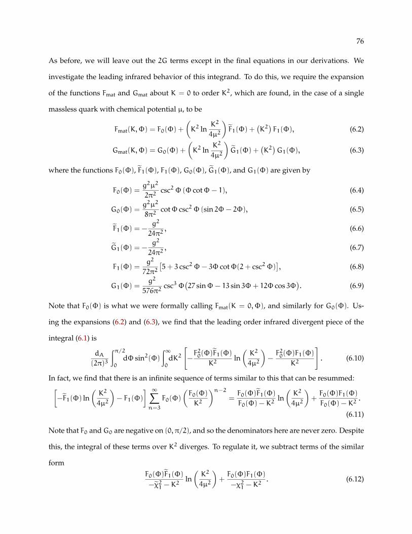
76
As before, we will leave out the 2G terms except in the final equations in our derivations. We
investigate the leading infrared behavior of this integrand. To do this, we require the expansion
of the functions Fmat and Gmat about K = 0 to order K2, which are found, in the case of a single
massless quark with chemical potential µ, to be
Fmat(K,Φ) = F0(Φ) +
(K2 ln
K2
4µ2
)F1(Φ) +
(K2)F1(Φ), (6.2)
Gmat(K,Φ) = G0(Φ) +
(K2 ln
K2
4µ2
)G1(Φ) +
(K2)G1(Φ), (6.3)
where the functions F0(Φ), F1(Φ), F1(Φ), G0(Φ), G1(Φ), and G1(Φ) are given by
F0(Φ) =g2µ2
2π2csc2Φ (Φ cotΦ− 1), (6.4)
G0(Φ) =g2µ2
8π2cotΦ csc2Φ (sin 2Φ− 2Φ), (6.5)
F1(Φ) = −g2
24π2, (6.6)
G1(Φ) = −g2
24π2, (6.7)
F1(Φ) =g2
72π2
[5+ 3 csc2Φ− 3Φ cotΦ(2+ csc2Φ)
], (6.8)
G1(Φ) =g2
576π2csc3Φ
(27 sinΦ− 13 sin 3Φ+ 12Φ cos 3Φ
). (6.9)
Note that F0(Φ) is what we were formally calling Fmat(K = 0,Φ), and similarly for G0(Φ). Us-
ing the expansions (6.2) and (6.3), we find that the leading order infrared divergent piece of the
integral (6.1) is
dA(2π)3
∫π/20
dΦ sin2(Φ)
∫∞0
dK2[−F20(Φ)F1(Φ)
K2ln(K2
4µ2
)−F20(Φ)F1(Φ)
K2
]. (6.10)
In fact, we find that there is an infinite sequence of terms similar to this that can be resummed:[−F1(Φ) ln
(K2
4µ2
)− F1(Φ)
] ∞∑n=3
F0(Φ)
(F0(Φ)
K2
)n−2=F0(Φ)F1(Φ)
F0(Φ) − K2ln(K2
4µ2
)+F0(Φ)F1(Φ)
F0(Φ) − K2.
(6.11)
Note that F0 andG0 are negative on (0, π/2), and so the denominators here are never zero. Despite
this, the integral of these terms over K2 diverges. To regulate it, we subtract terms of the similar
formF0(Φ)F1(Φ)
−χ21 − K2
ln(K2
4µ2
)+F0(Φ)F1(Φ)
−χ21 − K2. (6.12)

77
Here, χ1 and χ1 are two further fictitious mass scales that must also drop out of the calculation of
physical observables. The regulated integral over K2 evaluates to∫∞0
dK2F0(Φ)F1(Φ)
F0(Φ) − K2ln(K2
4µ2
)+F0(Φ)F1(Φ)
F0(Φ) − K2−F0(Φ)F1(Φ)
−χ21 − K2
ln(K2
4µ2
)−F0(Φ)F1(Φ)
−χ21 − K2
=1
2F0(Φ)2F1(Φ)
[ln2(−F0(Φ)
4µ2
)− ln2
(4µ2
χ21
)]+ F20(Φ)F1(Φ) ln
(−F0(Φ)
χ21
). (6.13)
Let us be clear what we have done. Just as in Sec. 3.1.8 above, we isolated a piece of the full
integral (6.1), namely the terms in Eq. (6.11), and regulated the result to obtain a finite answer. All
that is left is to perform the integral over Φ; this leads to the complete contributions to Ωplas at
orders g6 ln2 g,
Ω(1)plas
V=(g6 ln2 g
) dA(2π)3
∫π/20
dΦ sin2(Φ)
[2F0(Φ)2F1(Φ)
g6+ 2 · 2G0(Φ)2G1(Φ)
g6
], (6.14)
and g6 lng,
Ω(2)plas
V=(g6 lng
) dA(2π)3
∫π/20
dΦ sin2(Φ)
2F20(Φ)F1(Φ)
g6+2F20(Φ)F1(Φ)
g6ln
(−F0(Φ)
4µ2g2
)
+ 2·
[2G20(Φ)G1(Φ)
g6+2G20(Φ)G1(Φ)
g6ln
(−G0(Φ)
4µ2g2
)], (6.15)
with an additional piece contributing at order g6:
Ω(3)plas
V=(g6) dA(2π)3
∫π/20
dΦ sin2(Φ)
1
2
F20(Φ)F1(Φ)
g6
[ln2(−F0(Φ)
4µ2g2
)− ln2
(4µ2
χ21
)]
+F20(Φ)F1(Φ)
g6ln
(−F0(Φ)
χ21g2
)+G20(Φ)G1(Φ)
g6
[ln2(−G0(Φ)
4µ2g2
)− ln2
(4µ2
χ21
)]
+2G20(Φ)G1(Φ)
g6ln
(−G0(Φ)
χ21g2
). (6.16)
The final contribution at O(g6) is given by the remaining four terms of O(g6) contained in the
original integral (6.1) that were not included in the sum (6.11), plus the regulating terms that we

78
subtracted to obtain the finite integral (6.13) These are:
Ω(4)plas
V=(g6) dA(2π)3
∫π/20
dΦ sin2(Φ)
∫∞0
dK2F30(Φ)
3K4g6−F3mat(K,Φ)
3K4g6+ 2 ·
(G30(Φ)
3K4g6−G3mat(K,Φ)
3K4g6
)
+F0(Φ)F21(Φ)
g6
(1
−χ21 − K2+1
K2
)ln(K2
4µ2
)+F0(Φ)F21(Φ)
g6
(1
−χ21 − K2+1
K2
)+ 2 ·
[G0(Φ)G21(Φ)
g6
(1
−χ21 − K2+1
K2
)ln(K2
4µ2
)+G0(Φ)G21(Φ)
g6
(1
−χ21 − K2+1
K2
)].
(6.17)
Thus, to O(g6)
Ωplas = Ω(1)plas +Ω
(2)plas +Ω
(3)plas +Ω
(4)plas. (6.18)
For the single, massless quark flavor described above, some of these integrals can be done analyt-
ically, while others can be partially done:
Ω(1)plas
V= −
dAµ4
12 (2π)8g6 ln2 g, (6.19)
Ω(2)plas
V=
dAµ4
24 (2π)8
(35
6−7π2
24+16 ln2 23
+4 ln(4π3)
3− δ
)g6 lng. (6.20)
Here δ is defined exactly as in [39], namely,
δ ≡ 16
π
∫π/20
dx sin2 x
(1− x cot x
sin2 x
)2ln1− x cot x
sin2 x+1
2
(1−
1− x cot xsin2 x
)2ln
[1−
1− x cot xsin2 x
]
≈− 0.8563832093269428068483102329159403588472790971113576089930908673. (6.21)
Some of the remainingΦ integrals inΩ(3)plas +Ω
(4)plas can be done analytically too, but since we have
only managed to do the integral over K2 in Eq. (6.17) numerically due to the structure of Fmat and
Gmat, we do not reproduce them here. We do, however, include the numerical integrals for a single
massless quark flavor:
Ω(1)plas
V= −3.430676811637164× 10⁻⁸dAµ4g6 ln2 g, (6.22)
Ω(2)plas
V= 2.195772106112194× 10⁻⁷dAµ4g6 lng, (6.23)
Ω(3)plas +Ω
(4)plas
V= −3.088466558527530× 10⁻⁷dAµ4g6. (6.24)

79
6.2 Higher-order terms for multiple massless fermions
We now tackle multiple massless fermions. For nf massless quark flavors, the expansions
(6.2)-(6.3) become
Fmat(K,Φ) = F0(Φ) +
(∑f
K2 lnK2
4µ2f
)F1(Φ) +
(K2)F1(Φ), (6.25)
Gmat(K,Φ) = G0(Φ) +
(∑f
K2 lnK2
4µ2f
)G1(Φ) +
(K2)G1(Φ), (6.26)
with
F0(Φ) =g2µ2
2π2csc2Φ (Φ cotΦ− 1), (6.27)
G0(Φ) =g2µ2
8π2cotΦ csc2Φ (sin 2Φ− 2Φ), (6.28)
F1(Φ) = −g2
24π2, (6.29)
G1(Φ) = −g2
24π2, (6.30)
F1(Φ) =nfg
2
72π2
[5+ 3 csc2Φ− 3Φ cotΦ(2+ csc2Φ)
], (6.31)
G1(Φ) =nfg
2
576π2csc3Φ
(27 sinΦ− 13 sin 3Φ+ 12Φ cos 3Φ
), (6.32)
where we have defined µ2 =∑f µ2f . This means that the integrals forΩ(1)
plas-Ω(4)plas become
Ω(1)plas
V=(g6 ln2 g
) dA(2π)3
∫π/20
dΦ sin2(Φ)
[2F0(Φ)2F1(Φ)
g6+ 2 · 2G0(Φ)2G1(Φ)
g6
], (6.33)
Ω(2)plas
V=(g6 lng
) dA(2π)3
∫π/20
dΦ sin2(Φ)
2F20(Φ)F1(Φ)
g6+2F20(Φ)F1(Φ)
g6
∑f
ln
(−F0(Φ)
4µ2fg2
)
+ 2
[2G20(Φ)G1(Φ)
g6+2G20(Φ)G1(Φ)
g6
∑f
ln
(−G0(Φ)
4µ2fg2
)], (6.34)
Ω(3)plas
V=(g6) dA(2π)3
∫π/20
dΦ sin2(Φ)
1
2
F20(Φ)F1(Φ)
g6
∑f
[ln2(−F0(Φ)
4µ2fg2
)− ln2
(4µ2fχ21
)]
+F20(Φ)F1(Φ)
g6ln
(−F0(Φ)
χ21g2
)+G20(Φ)G1(Φ)
g6
∑f
[ln2(−G0(Φ)
4µ2fg2
)− ln2
(4µ2fχ21
)]
+2G20(Φ)G1(Φ)
g6ln
(−G0(Φ)
χ21g2
), (6.35)
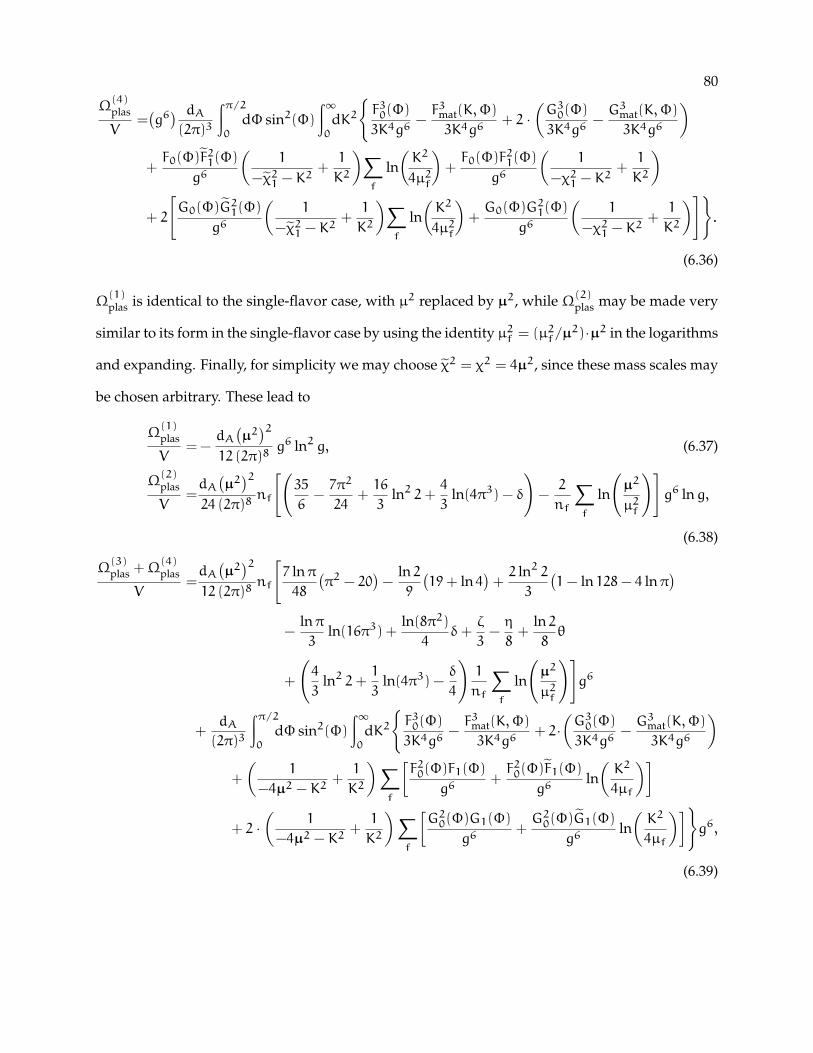
80
Ω(4)plas
V=(g6) dA(2π)3
∫π/20
dΦ sin2(Φ)
∫∞0
dK2F30(Φ)
3K4g6−F3mat(K,Φ)
3K4g6+ 2 ·
(G30(Φ)
3K4g6−G3mat(K,Φ)
3K4g6
)
+F0(Φ)F21(Φ)
g6
(1
−χ21 − K2+1
K2
)∑f
ln(K2
4µ2f
)+F0(Φ)F21(Φ)
g6
(1
−χ21 − K2+1
K2
)
+ 2
[G0(Φ)G21(Φ)
g6
(1
−χ21 − K2+1
K2
)∑f
ln(K2
4µ2f
)+G0(Φ)G21(Φ)
g6
(1
−χ21 − K2+1
K2
)].
(6.36)
Ω(1)plas is identical to the single-flavor case, with µ2 replaced by µ2, while Ω(2)
plas may be made very
similar to its form in the single-flavor case by using the identity µ2f = (µ2f/µ2)·µ2 in the logarithms
and expanding. Finally, for simplicity we may choose χ2 = χ2 = 4µ2, since these mass scales may
be chosen arbitrary. These lead to
Ω(1)plas
V=−
dA(µ2)2
12 (2π)8g6 ln2 g, (6.37)
Ω(2)plas
V=dA(µ2)2
24 (2π)8nf
[(35
6−7π2
24+16
3ln2 2+
4
3ln(4π3) − δ
)−2
nf
∑f
ln
(µ2
µ2f
)]g6 lng,
(6.38)
Ω(3)plas +Ω
(4)plas
V=dA(µ2)2
12 (2π)8nf
[7 lnπ48
(π2 − 20
)−
ln 29
(19+ ln 4
)+2 ln2 23
(1− ln 128− 4 lnπ
)−
lnπ3
ln(16π3) +ln(8π2)4
δ+ζ
3−η
8+
ln 28θ
+
(4
3ln2 2+
1
3ln(4π3) −
δ
4
)1
nf
∑f
ln
(µ2
µ2f
)]g6
+dA
(2π)3
∫π/20
dΦ sin2(Φ)
∫∞0
dK2F30(Φ)
3K4g6−F3mat(K,Φ)
3K4g6+ 2·
(G30(Φ)
3K4g6−G3mat(K,Φ)
3K4g6
)
+
(1
−4µ2 − K2+1
K2
)∑f
[F20(Φ)F1(Φ)
g6+F20(Φ)F1(Φ)
g6ln(K2
4µf
)]
+ 2 ·(
1
−4µ2 − K2+1
K2
)∑f
[G20(Φ)G1(Φ)
g6+G20(Φ)G1(Φ)
g6ln(K2
4µf
)]g6,
(6.39)

81
where the final contribution to the O(g6) term has not yet been analytically evaluated. Here, δ is
as defined above, and ζ, η, and θ are defined as the following integrals:
ζ ≡ 4
π
∫π/20
dx sin2 x
[5+ 3 csc2 x− 3x cot x
(2+ csc2 x
)](1− x cot xsin2 x
)2ln1− x cot x
sin2 x
+1
16
12x cos 3x+ 27 sin x− 13 sin 3xsin3 x
(1−
1− x cot xsin2 x
)2ln[1−
1− x cot xsin2 x
]
≈− 0.663092750844561011343238360662050961220020228051329183397267483, (6.40)
η ≡ 16
π
∫π/20
dx sin2 x
(1− x cot x
sin2 x
)2ln2
1− x cot xsin2 x
+1
2
(1−
1− x cot xsin2 x
)2ln2[1−
1− x cot xsin2 x
]
≈ 0.5486478397145719666196365740853549094616061512122073020649720940, (6.41)
θ ≡ 16
π
∫π/20
dx sin2 x
(1−
1− x cot xsin2 x
)2ln[1−
1− x cot xsin2 x
]
≈ − 0.5113655867492375453885515179665998062769227625253022640530703657, (6.42)
which are all quite similar to the defining integral for δ.
6.3 Contribution of the two-loop self-energy
We also note here that there will be a contribution to the ring sum at O(g6 lng) coming from
an O(g4) contribution to Πµν(K = 0,Φ). This can be seen directly from Eq. (3.91). Suppose that
Fmat(K = 0,Φ) is of the form
Fmat(K = 0,Φ) = F2(Φ)g2 + F4(Φ)g4 (6.43)
with Gmat(K = 0,Φ) of an analogous form. Then the F2mat(K = 0,Φ) term in (3.91) will contain a
term of O(g6), namely
2F2(Φ)F4(Φ)g6, (6.44)
which contributes a term
Ω2-loopplas
V=2dAg
6 lng(2π)3
∫π/20
dΦ sin2(Φ)[F2(Φ)F4(Φ) + 2G2(Φ)G4(Φ)
](6.45)

82
to the pressure. Any other contributions to Ωplas coming from the O(g4) piece of Πµν will be
of at least O(g8 ln2 g) (coming from cross terms in the O(g6 ln2 g) piece derived above). This
contribution to the O(g6 lng) piece of the zero-temperature pQCD pressure is currently being
worked on by the author and collaborators. This contribution, in fact, is the only other contribution
to the full O(g6 lng) result. (This follows from the fact that all the other diagrams that contribute
at O(g6) are infrared-safe, and it is only through infrared divergences of individual diagrams that
the non-analytic logarithmic terms can arise.) The full O(g6) result, however, has many more
diagrams that contribute, which makes that term much more formidable to calculate.
Note, however, that an O(g6 ln2 g) result cannot be reproduced by higher-order terms in
the gluon self-energy, since the lowest-order contribution from the two-loop self-energy enters at
O(g6 lng). This means that the O(g6 ln2 g) contribution given in this chapter in Eq. (6.37) is the
full contribution at that order, and by itself constitutes a quantitative improvement to the pQCD
pressure at T = 0.

CHAPTER 7
CONCLUSIONS
In this thesis, we have advocated for thermodynamic matching as a way to constrain the
zero-temperature QCD EoS in the intermediate, non-perturbative regime, corresponding roughly
to µ ∈ (0.97 GeV, 2.6 GeV). Such a matching procedure can be carried out with various levels of
sophistication, as has been illustrated in Chap. 4. The simplicity of the approach is noteworthy,
for one may quantitatively constrain the intermediate EoS with little or no knowledge of the mi-
crophysics in the regime of interest. This is of course not to say that we are not interested in the
microphysics, but a quantitative constraint of any non-perturbative physical property is a signifi-
cant step.
We began this thesis with three goals in mind, beyond simply identifying thermodynamic
matching as a legitimate approach to physically interesting problems: First, we desired a method
to check if such a simplistic approach is valid; second, we wished to extend applications of the
state-of-the-art QCD EoS of Refs. [1, 11] to rotating NSs; and third, we wished to make quanti-
tative improvements to the zero-temperature pQCD pressure. All three of these goals have been
accomplished.
On the first topic, we have shown in Sec. 4.1 that EoS matching in certain SU(N) (“QCD-
like”) theories can be verified or refuted by lattice simulations. In particular, the theories (N,nf) =
(2, 2) with quarks in the fundamental representation and (N,nf) = (4, 2) with quarks in the two-

84
index, antisymmetric representation can both be simulated on the lattice without a sign prob-
lem. We have produced matching results within the HRG+pQCD framework for the pressure
and trace anomaly along the T - and µ-axes in both of these theories, as well as in the theories
(N,nf) = (4, 2) and (3, 3) with quarks in the fundamental representation. The last of these the-
ories is an approximation to real-world QCD. While some aspects of our HRG+pQCD study are
systematically improvable, we expect the results in Sec. 4.1 to be sufficiently robust that a direct
comparison with future lattice-QCD studies in the aforementioned theories could validate or rule
out the HRG+pQCD method.
On the second topic, we have extended the results of Refs. [1, 11] to rotating NSs. We iden-
tified B1516+02B as a NS that could place more stringent constraints on the QCD EoS if its mass
could be determined more precisely. We also identified f = 882 Hz as the maximum allowed
rotation rate for a NS (or f = 780 Hz if restricted to a 1.4M star). In addition, we derived the
allowed equatorial radius vs. frequency band of a 1.4M star, which serves as a prediction for
astronomers, and can be used in the future to further constrain the QCD EoS. Lastly, we identified
the binary pulsar PSR J0737-3039A as a physical object of extreme interest: a measurement of the
moment of inertia of this pulsar, even to low precision, would significantly constrain the QCD EoS
band of Refs. [1, 11].
On the third and final topic, we have calculated the full O(g6 ln2 g) piece of the pQCD pres-
sure at T = 0, along with a significant portion of the O(g6 lng) piece and even a portion of the
O(g6) piece. These improvements can be incorporated into future matching work to improve the
entire zero-temperature QCD EoS. In addition, these improvements are of interest in their own
right, for they constitute fundamental improvements to our knowledge of pQCD at T = 0.
QCD matching is therefore an effective, verifiable, and systematically improvable method to
explore non-perturbative regimes of the QCD EoS. It provides a window into regions of the QCD
phase diagram where, as yet, no microphysical descriptions exist. This makes it a powerful, con-
trolled tool for probing areas of the universe that are currently inaccessible to direct, microscopic
calculations.

BIBLIOGRAPHY
[1] A. Kurkela, E.S. Fraga, J. Schaffner-Bielich, and A. Vuorinen. “Constraining neutron starmatter with Quantum Chromodynamics”. Astrophys.J. 789 (2014), p. 127. arXiv: 1402.6618(astro-ph.HE).
[2] J. Beringer et al. (Particle Data Group). “Review of Particle Physics (RPP)”. Phys. Rev. D86(2012), p. 010001.
[3] E. Epelbaum, H.-W. Hammer, and U.-G. Meissner. “Modern Theory of Nuclear Forces”. Rev.Mod. Phys. 81 (2009), pp. 1773–1825. arXiv: 0811.1338 (nucl-th).
[4] R. Machleidt and D.R. Entem. “Chiral effective field theory and nuclear forces”. Phys. Rept.503 (2011), pp. 1–75. arXiv: 1105.2919 (nucl-th).
[5] K. Fukushima and C. Sasaki. “The phase diagram of nuclear and quark matter at highbaryon density”. Prog. Part. Nucl. Phys. 72 (2013), pp. 99–154. arXiv: 1301.6377 (hep-ph).
[6] D. Page and S. Reddy. “Dense Matter in Compact Stars: Theoretical Developments and Ob-servational Constraints”. Ann. Rev. Nucl. Part. Sci. 56 (2006), pp. 327–374. arXiv: astro-ph/0608360 (astro-ph).
[7] U. Lombardo and H.J. Schulze. “Superfluidity in neutron star matter”. Lect. Notes Phys. 578(2001), pp. 30–53. arXiv: astro-ph/0012209 (astro-ph).
[8] A.R. Bodmer. “Collapsed nuclei”. Phys. Rev. D4 (1971), pp. 1601–1606.
[9] E. Witten. “Cosmic Separation of Phases”. Phys. Rev. D30 (1984), pp. 272–285.
[10] A. Kurkela, P. Romatschke, and A. Vuorinen. “Cold Quark Matter”. Phys.Rev. D81 (2010),p. 105021. arXiv: 0912.1856 (hep-ph).
[11] E.S. Fraga, A. Kurkela, and A. Vuorinen. “Neutron star structure from QCD”. Eur. Phys. J.A52.3 (2016), p. 49. arXiv: 1508.05019 (nucl-th).
[12] A. Kurkela and A. Vuorinen. “Cool quark matter”. Phys. Rev. Lett. 117.4 (2016), p. 042501.arXiv: 1603.00750 (hep-ph).
[13] H. Shen, H. Toki, K. Oyamatsu, and K. Sumiyoshi. “Relativistic equation of state of nuclearmatter for supernova and neutron star”. Nucl. Phys. A637 (1998), pp. 435–450. arXiv: nucl-th/9805035 (nucl-th).

86
[14] M.G. Alford, A. Schmitt, K. Rajagopal, and T. Schäfer. “Color superconductivity in densequark matter”. Rev.Mod.Phys. 80 (2008), pp. 1455–1515. arXiv: 0709.4635 (hep-ph).
[15] Y. Aoki, G. Endrodi, Z. Fodor, S.D. Katz, and K.K. Szabo. “The Order of the quantum chro-modynamics transition predicted by the standard model of particle physics”. Nature 443(2006), pp. 675–678. arXiv: hep-lat/0611014 (hep-lat).
[16] I. Montvay and G. Munster. Quantum fields on a lattice. Cambridge University Press, 1997.
[17] J.B. Kogut and M.A. Stephanov. “The phases of quantum chromodynamics: From confine-ment to extreme environments”. Camb. Monogr. Part. Phys. Nucl. Phys. Cosmol. 21 (2004),pp. 1–364.
[18] C.R. Allton, S. Ejiri, S.J. Hands, O. Kaczmarek, F. Karsch, E. Laermann, C. Schmidt, and L.Scorzato. “The QCD thermal phase transition in the presence of a small chemical potential”.Phys. Rev. D66 (2002), p. 074507. arXiv: hep-lat/0204010 (hep-lat).
[19] P. de Forcrand and O. Philipsen. “The QCD phase diagram for small densities from imag-inary chemical potential”. Nucl. Phys. B642 (2002), pp. 290–306. arXiv: hep-lat/0205016(hep-lat).
[20] M. Cristoforetti, F. Di Renzo, and L. Scorzato (AuroraScience Collaboration). “New ap-proach to the sign problem in quantum field theories: High density QCD on a Lefschetzthimble”. Phys.Rev. D86 (2012), p. 074506. arXiv: 1205.3996 (hep-lat).
[21] G. Aarts, L. Bongiovanni, E. Seiler, D. Sexty, and I.-O. Stamatescu. “Controlling complexLangevin dynamics at finite density”. Eur.Phys.J. A49 (2013), p. 89. arXiv: 1303.6425 (hep-lat).
[22] D. Sexty. “Simulating full QCD at nonzero density using the complex Langevin equation”.Phys.Lett. B729 (2014), pp. 108–111. arXiv: 1307.7748 (hep-lat).
[23] G. Aarts, E. Seiler, D. Sexty, and I.-O. Stamatescu. “Simulating QCD at nonzero baryon den-sity to all orders in the hopping parameter expansion”. Phys. Rev. D90.11 (2014), p. 114505.arXiv: 1408.3770 (hep-lat).
[24] G. Aarts, F. Attanasio, B. Jäger, E. Seiler, D. Sexty, and I.-O. Stamatescu. “QCD at nonzerochemical potential: recent progress on the lattice”. AIP Conf. Proc. 1701 (2016), p. 020001.arXiv: 1412.0847 (hep-lat).
[25] P. de Forcrand, J. Langelage, O. Philipsen, and W. Unger. “The lattice QCD phase diagramin and away from the strong coupling limit”. Phys.Rev.Lett. 113 (2014), p. 152002. arXiv:1406.4397 (hep-lat).
[26] G. Aarts. “Introductory lectures on lattice QCD at nonzero baryon number”. J. Phys. Conf.Ser. 706.2 (2016), p. 022004. arXiv: 1512.05145 (hep-lat).
[27] P.J. Siemens. “Liquid-gas phase transition in nuclear matter”. Nature 305.5933 (Sept. 1983),pp. 410–412.

87
[28] T. Tatsumi, N. Yasutake, and T. Maruyama. Mixed phases during the phase transitions. 2011.arXiv: 1107.0804 (nucl-th).
[29] M. Srednicki and L. Susskind. “Alternative Patterns of Chiral Symmetry Breaking in QCD”.Nucl. Phys. B187 (1981), pp. 93–102.
[30] N. Brambilla et al. “QCD and Strongly Coupled Gauge Theories: Challenges and Perspec-tives”. Eur. Phys. J. C74.10 (2014), p. 2981. arXiv: 1404.3723 (hep-ph).
[31] J.I. Kapusta and C. Gale. Finite-temperature field theory: Principles and applications. CambridgeUniversity Press, 2011, p. 442.
[32] M. Laine and A. Vuorinen. “Basics of Thermal Field Theory”. Lect. Notes Phys. 925 (2016),pp.1–281.
[33] M.L. Bellac. Thermal Field Theory. Cambridge University Press, 2011.
[34] M.D. Schwartz. Quantum Field Theory and the Standard Model. Cambridge University Press,2014.
[35] J. Ellis. “TikZ-Feynman: Feynman diagrams with TikZ” (2016). arXiv: 1601.05437 (hep-ph).
[36] J.I. Kapusta. “Infrared Properties of Quark Gas”. Phys. Rev. D20 (1979), p. 989.
[37] T. Toimela. “Perturbative QED and QCD at Finite Temperatures and Densities”. Int. J. Theor.Phys. 24 (1985). [Erratum: Int. J. Theor. Phys.26,1021(1987)], p. 901.
[38] B. Freedman and L. McLerran. “Fermions and Gauge Vector Mesons at Finite Temperatureand Density. 3. The Ground State Energy of a Relativistic Quark Gas”. Phys. Rev. D16 (1977),p. 1169.
[39] A. Vuorinen. “The Pressure of QCD at finite temperatures and chemical potentials”. Phys.Rev.D68 (2003), p. 054017. arXiv: hep-ph/0305183 (hep-ph).
[40] S. Borsanyi, G. Endrodi, Z. Fodor, A. Jakovac, S.D. Katz, S. Krieg, C. Ratti, and K.K. Szabo.“The QCD equation of state with dynamical quarks”. JHEP 11 (2010), p. 077. arXiv: 1007.2580 (hep-lat).
[41] S. Borsanyi, Z. Fodor, C. Hoelbling, S.D. Katz, S. Krieg, and K.K. Szabo. “Full result for theQCD equation of state with 2+1 flavors”. Phys.Lett. B730 (2014), pp. 99–104. arXiv: 1309.5258(hep-lat).
[42] A. Bazavov et al. (HotQCD Collaboration). “Equation of state in (2+1)-flavor QCD”. Phys.Rev.D90.9 (2014), p. 094503. arXiv: 1407.6387 (hep-lat).
[43] J. Langelage, G. Munster, and O. Philipsen. “Strong coupling expansion for finite tempera-ture Yang-Mills theory in the confined phase”. JHEP 0807 (2008), p. 036. arXiv: 0805.1163(hep-lat).

88
[44] S. Hands, S. Kim, and J.-I. Skullerud. “Deconfinement in dense 2-color QCD”. Eur.Phys.J.C48 (2006), p. 193. arXiv: hep-lat/0604004 (hep-lat).
[45] J. Kogut, M.A. Stephanov, D. Toublan, J. Verbaarschot, and A. Zhitnitsky. “QCD - like the-ories at finite baryon density”. Nucl.Phys. B582 (2000), pp. 477–513. arXiv: hep-ph/0001171(hep-ph).
[46] J.F. Donoghue, E. Golowich, and B.R. Holstein. “Dynamics of the standard model”. Camb.Monogr. Part. Phys. Nucl. Phys. Cosmol. (2014), pp. 1–540.
[47] S. Weinberg. The quantum theory of fields. Vol. 2: Modern applications. Cambridge UniversityPress, 2013.
[48] T. Gorda and P. Romatschke. “Equation of state in two-, three-, and four-color QCD atnonzero temperature and density”. Phys. Rev. D92.1 (2015), p. 014019. arXiv: 1412 . 6712(hep-ph).
[49] M. Laine and Y. Schroder. “Quark mass thresholds in QCD thermodynamics”. Phys.Rev. D73(2006), p. 085009. arXiv: hep-ph/0603048 (hep-ph).
[50] P. Huovinen and P. Petreczky. “QCD Equation of State and Hadron Resonance Gas”. Nucl.Phys.A837 (2010), pp. 26–53. arXiv: 0912.2541 (hep-ph).
[51] K. Kajantie, M. Laine, K. Rummukainen, and Y. Schroder. “The Pressure of hot QCD up tog6 ln(1/g)”. Phys.Rev. D67 (2003), p. 105008. arXiv: hep-ph/0211321 (hep-ph).
[52] K. Kajantie, M. Laine, K. Rummukainen, and Y. Schroder. “Four loop vacuum energy densityof the SU(N(c)) + adjoint Higgs theory”. JHEP 0304 (2003), p. 036. arXiv: hep-ph/0304048(hep-ph).
[53] J. Blaizot, E. Iancu, and A. Rebhan. “On the apparent convergence of perturbative QCD athigh temperature”. Phys.Rev. D68 (2003), p. 025011. arXiv: hep-ph/0303045 (hep-ph).
[54] N. Haque, A. Bandyopadhyay, J.O. Andersen, M.G. Mustafa, M. Strickland, et al. “Three-loop HTLpt thermodynamics at finite temperature and chemical potential”. JHEP 1405 (2014),p. 027. arXiv: 1402.6907 (hep-ph).
[55] E. Braaten and A. Nieto. “Free energy of QCD at high temperature”. Phys.Rev. D53 (1996),pp. 3421–3437. arXiv: hep-ph/9510408 (hep-ph).
[56] T. van Ritbergen, J. Vermaseren, and S. Larin. “The Four loop beta function in quantumchromodynamics”. Phys.Lett. B400 (1997), pp. 379–384. arXiv: hep-ph/9701390 (hep-ph).
[57] M.G. Alford, K. Rajagopal, and F. Wilczek. “Color flavor locking and chiral symmetry break-ing in high density QCD”. Nucl.Phys. B537 (1999), pp. 443–458. arXiv: hep-ph/9804403 (hep-ph).
[58] M. Orsaria, S. Duarte, and H. Rodrigues. “Color flavor locked phase transition in strangequark matter”. Braz.J.Phys. 37 (2007), pp. 20–22.

89
[59] K. Olive et al. (Particle Data Group). “Review of Particle Physics”. Chin.Phys. C38 (2014),p. 090001. arXiv: 1412.1408 (astro-ph.CO).
[60] H.B. Meyer and M.J. Teper. “Glueball Regge trajectories and the pomeron: A Lattice study”.Phys.Lett. B605 (2005), pp. 344–354. arXiv: hep-ph/0409183 (hep-ph).
[61] B. Lucini and G. Moraitis. “The Running of the coupling in SU(N) pure gauge theories”.Phys.Lett. B668 (2008), pp. 226–232. arXiv: 0805.2913 (hep-lat).
[62] P. Fritzsch, F. Knechtli, B. Leder, M. Marinkovic, S. Schaefer, et al. “The strange quark massand Lambda parameter of two flavor QCD”. Nucl.Phys. B865 (2012), pp. 397–429. arXiv:1205.5380 (hep-lat).
[63] G.S. Bali, F. Bursa, L. Castagnini, S. Collins, L. Del Debbio, et al. “Mesons in large-N QCD”.JHEP 1306 (2013), p. 071. arXiv: 1304.4437 (hep-lat).
[64] S. Hands, P. Sitch, and J.-I. Skullerud. “Hadron Spectrum in a Two-Colour Baryon-RichMedium”. Phys.Lett. B662 (2008), pp. 405–412. arXiv: 0710.1966 (hep-lat).
[65] R. Lewis, C. Pica, and F. Sannino. “Light Asymmetric Dark Matter on the Lattice: SU(2)Technicolor with Two Fundamental Flavors”. Phys.Rev. D85 (2012), p. 014504. arXiv: 1109.3513 (hep-ph).
[66] G.S. Adkins, C.R. Nappi, and E. Witten. “Static Properties of Nucleons in the Skyrme Model”.Nucl.Phys. B228 (1983), p. 552.
[67] E.E. Jenkins. “Baryon hyperfine mass splittings in large N QCD”. Phys.Lett. B315 (1993),pp. 441–446. arXiv: hep-ph/9307244 (hep-ph).
[68] T. DeGrand. “Lattice baryons in the 1/N expansion”. Phys.Rev. D86 (2012), p. 034508. arXiv:1205.0235 (hep-lat).
[69] T. Appelquist et al. (Lattice Strong Dynamics (LSD) Collaboration). “Composite bosonicbaryon dark matter on the lattice: SU(4) baryon spectrum and the effective Higgs inter-action”. Phys.Rev. D89 (2014), p. 094508. arXiv: 1402.6656 (hep-lat).
[70] T. DeGrand, Y. Liu, E.T. Neil, Y. Shamir, and B. Svetitsky. “Spectroscopy of SU(4) gaugetheory with two flavors of sextet fermions”. Phys. Rev. D91 (2015), p. 114502. arXiv: 1501.05665 (hep-lat).
[71] T. DeGrand, Y. Liu, E.T. Neil, Y. Shamir, and B. Svetitsky. “Spectroscopy of SU(4) latticegauge theory with fermions in the two index anti-symmetric representation”. PoS LAT-TICE2014 (2014), p. 275. arXiv: 1412.4851 (hep-lat).
[72] S. Bolognesi. “Baryons and Skyrmions in QCD with Quarks in Higher Representations”.Phys.Rev. D75 (2007), p. 065030. arXiv: hep-th/0605065 (hep-th).
[73] M.E. Peskin. “The Alignment of the Vacuum in Theories of Technicolor”. Nucl.Phys. B175(1980), pp. 197–233.

90
[74] M. Panero. “Thermodynamics of the QCD plasma and the large-N limit”. Phys.Rev.Lett. 103(2009), p. 232001. arXiv: 0907.3719 (hep-lat).
[75] P. Bedaque and A.W. Steiner. “Sound velocity bound and neutron stars”. Phys. Rev. Lett.114.3 (2015), p. 031103. arXiv: 1408.5116 (nucl-th).
[76] The results may be obtained from the web page of one of the authors of the original paperfrom which this section is taken, http://hep.itp.tuwien.ac.at/~paulrom/.
[77] I. Tews, T. Krüger, K. Hebeler, and A. Schwenk. “Neutron matter at next-to-next-to-next-to-leading order in chiral effective field theory”. Phys. Rev. Lett. 110.3 (2013), p. 032504. arXiv:1206.0025 (nucl-th).
[78] E.S. Fraga, A. Kurkela, and A. Vuorinen. “Interacting quark matter equation of state forcompact stars”. Astrophys. J. 781.2 (2014), p. L25. arXiv: 1311.5154 (nucl-th).
[79] P. Demorest, T. Pennucci, S. Ransom, M. Roberts, and J. Hessels. “Shapiro Delay Measure-ment of A Two Solar Mass Neutron Star”. Nature 467 (2010), pp. 1081–1083. arXiv: 1010.5788(astro-ph.HE).
[80] J. Antoniadis et al. “A Massive Pulsar in a Compact Relativistic Binary”. Science 340 (2013),p. 6131. arXiv: 1304.6875 (astro-ph.HE).
[81] S. Abbar, J. Carlson, H. Duan, and S. Reddy. “Quantum Monte Carlo calculations of thethermal conductivity of neutron star crusts”. Phys. Rev. C92.4 (2015), p. 045809. arXiv: 1503.01696 (astro-ph.HE).
[82] K. Hebeler and A. Schwenk. “Chiral three-nucleon forces and neutron matter”. Phys. Rev.C82 (2010), p. 014314. arXiv: 0911.0483 (nucl-th).
[83] O. Benhar, V. Ferrari, L. Gualtieri, and S. Marassi. “Perturbative approach to the structureof rapidly rotating neutron stars”. Phys. Rev. D72 (2005), p. 044028. arXiv: gr-qc/0504068(gr-qc).
[84] F. Cipolletta, C. Cherubini, S. Filippi, J.A. Rueda, and R. Ruffini. “Fast Rotating NeutronStars with Realistic Nuclear Matter Equation of State”. Phys. Rev. D92.2 (2015), p. 023007.arXiv: 1506.05926 (astro-ph.SR).
[85] P. Haensel, M. Bejger, M. Fortin, and L. Zdunik. “Rotating neutron stars with exotic cores:masses, radii, stability”. Eur. Phys. J. A52.3 (2016), p. 59. arXiv: 1601.05368 (astro-ph.HE).
[86] M. Kramer and N. Wex. “The double pulsar system: A unique laboratory for gravity”. Class.Quant. Grav. 26 (2009), p. 073001.
[87] I.A. Morrison, T.W. Baumgarte, S.L. Shapiro, and V.R. Pandharipande. “The Moment of iner-tia of the binary pulsar J0737-3039A: Constraining the nuclear equation of state”. Astrophys.J. 617 (2004), pp. L135–L138. arXiv: astro-ph/0411353 (astro-ph).

91
[88] T. Gorda. “Global properties of rotating neutron stars with QCD equations of state” (2016).arXiv: 1605.08067 (astro-ph.HE). (Soon to be published in Astrophys J.)
[89] S.M. Carroll. Spacetime and geometry: An introduction to general relativity. San Francisco, USA:Addison-Wesley, 2004, p. 513.
[90] B. Carter. “Killing horizons and orthogonally transitive groups in space-time”. J. Math. Phys.10 (1969), pp. 70–81.
[91] A. Papapetrou. “Champs gravitationnels stationnaires a symetrie axiale”. Ann. Inst. H. PoincarePhys. Theor. IV (1966), pp. 83–105.
[92] T. Nozawa, N. Stergioulas, E. Gourgoulhon, and Y. Eriguchi. “Construction of highly accu-rate models of rotating neutron stars: Comparison of three different numerical schemes”.Astron. Astrophys. Suppl. Ser. 132 (1998), p. 431. arXiv: gr-qc/9804048 (gr-qc).
[93] H. Komatsu, Y. Eriguchi, and I. Hachisu. “Rapidly rotating general relativistic stars. I - Nu-merical method and its application to uniformly rotating polytropes”. Mon. Not. Roy. Astron.Soc. 237 (1989), pp. 355–379.
[94] N. Stergioulas and J. Friedman. “Comparing models of rapidly rotating relativistic starsconstructed by two numerical methods”. Astrophys. J. 444 (1995), p. 306. arXiv: astro-ph/9411032 (astro-ph). Code available at: http://www.gravity.phys.uwm.edu/rns/.
[95] J.W.T. Hessels, S.M. Ransom, I.H. Stairs, P.C.C. Freire, V.M. Kaspi, and F. Camilo. “A radiopulsar spinning at 716-hz”. Science 311 (2006), pp. 1901–1904. arXiv: astro - ph / 0601337(astro-ph).
[96] A. Kurkela, P. Romatschke, A. Vuorinen, and B. Wu. “Looking inside neutron stars: Micro-scopic calculations confront observations” (2010). arXiv: 1006.4062 (astro-ph.HE).
[97] J.M. Lattimer and B.F. Schutz. “Constraining the equation of state with moment of inertiameasurements”. Astrophys. J. 629 (2005), pp. 979–984. arXiv: astro-ph/0411470 (astro-ph).
[98] M. Bejger, T. Bulik, and P. Haensel. “Moments of inertia of the binary pulsars J0737-3039A,Band the dense matter EOS”. Mon. Not. Roy. Astron. Soc. 364 (2005), p. 635. arXiv: astro-ph/0508105 (astro-ph).
[99] C.A. Raithel, F. Ozel, and D. Psaltis. “Model-Independent Inference of Neutron Star Radiifrom Moment of Inertia Measurements”. Phys. Rev. C93.3 (2016). [Addendum: Phys. Rev.C93,no.4, 049905(2016)], p. 032801. arXiv: 1603.06594 (astro-ph.HE).

APPENDIX A
PARTICLE TABLES
MesonsMass/
√σ Spin Isospin
0.00 0 11.43 0 01.60 1 11.86 1 02.79 1 03.02 2 03.06 1 03.08 0 03.10 1 13.14 2 13.25 1 13.26 0 03.38 1 03.50 0 13.50 0 1
Mesons (continued)Mass/
√σ Spin Isospin
3.65 1 13.92 2 03.93 1 03.98 2 13.98 3 04.02 3 14.05 1 14.25 0 14.25 0 04.35 1 14.35 1 04.86 4 14.88 4 05.00 1 15.00 1 0
BaryonsMass/
√σ Spin Isospin
0.00 0 01.43 0 01.86 1 12.79 1 13.26 0 03.06 1 03.02 2 03.92 2 03.93 1 13.98 3 14.88 4 03.08 0 03.38 1 15.00 1 14.25 0 04.35 1 0
TABLE A.1: The included particle spectrum in the two-color fundamental theory.

93Mesons
Mass/√σ Spin Isospin
0.00 0 11.43 0 01.83 1 11.86 1 02.33 0 12.79 1 02.94 1 13.00 1 13.02 2 03.06 1 03.08 0 03.10 0 13.14 2 13.26 0 03.38 1 03.45 1 13.45 0 13.90 1 13.92 2 03.93 1 03.98 2 1
Mesons (continued)Mass/
√σ Spin Isospin
3.98 3 04.02 3 14.05 1 14.25 0 04.35 1 04.86 4 14.88 4 05.00 1 15.00 1 0
BaryonsMass/
√σ Spin Isospin
2.84 0 13.05 1 33.47 2 52.84 0 53.05 1 53.47 2 53.05 1 33.47 2 34.10 3 3
TABLE A.2: The included particle spectrum in the four-color fundamental theory.
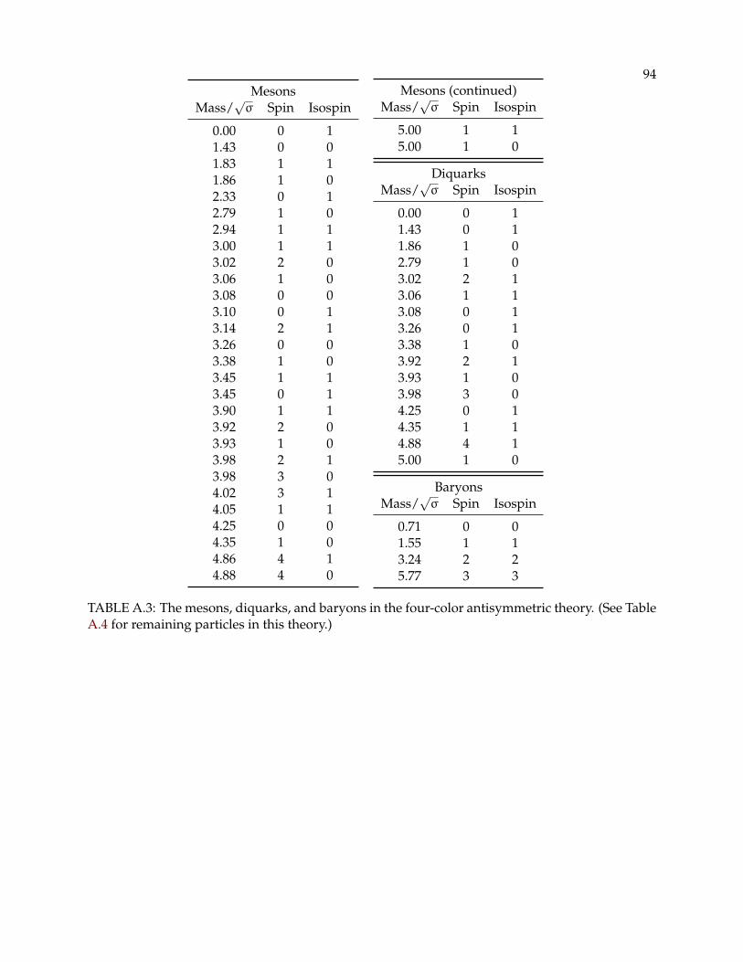
94Mesons
Mass/√σ Spin Isospin
0.00 0 11.43 0 01.83 1 11.86 1 02.33 0 12.79 1 02.94 1 13.00 1 13.02 2 03.06 1 03.08 0 03.10 0 13.14 2 13.26 0 03.38 1 03.45 1 13.45 0 13.90 1 13.92 2 03.93 1 03.98 2 13.98 3 04.02 3 14.05 1 14.25 0 04.35 1 04.86 4 14.88 4 0
Mesons (continued)Mass/
√σ Spin Isospin
5.00 1 15.00 1 0
DiquarksMass/
√σ Spin Isospin
0.00 0 11.43 0 11.86 1 02.79 1 03.02 2 13.06 1 13.08 0 13.26 0 13.38 1 03.92 2 13.93 1 03.98 3 04.25 0 14.35 1 14.88 4 15.00 1 0
BaryonsMass/
√σ Spin Isospin
0.71 0 01.55 1 13.24 2 25.77 3 3
TABLE A.3: The mesons, diquarks, and baryons in the four-color antisymmetric theory. (See TableA.4 for remaining particles in this theory.)

95
Four-quark objectsm/
√σ gS gI
0.00 1 11.43 1 11.86 3 32.79 3 32.86 1 13.02 5 53.06 3 33.08 1 13.26 1 13.29 3 33.38 3 33.72 9 93.92 5 53.93 3 33.98 7 74.21 3 34.25 1 14.35 3 34.45 5 54.49 3 34.51 1 14.65 9 94.69 1 14.81 3 34.88 9 94.89 15 154.92 9 94.95 3 35.00 3 35.12 3 35.24 9 95.35 5 5
(continued)m/
√σ gS gI
5.36 3 35.40 7 75.57 9 95.68 1 15.78 18 185.79 9 95.81 15 155.84 21 215.85 9 95.87 3 36.05 28 286.08 15 156.11 5 56.11 3 36.12 9 96.14 3 36.17 10 106.21 9 96.29 5 56.31 9 96.32 3 36.35 1 16.40 15 156.43 3 36.44 9 96.46 3 36.52 1 16.64 3 36.70 15 156.71 9 96.74 27 276.76 30 30
(continued)m/
√σ gS gI
6.86 9 96.94 25 256.95 15 156.98 15 156.99 9 97.00 40 407.01 3 37.04 24 247.06 7 77.14 9 97.18 5 57.19 3 37.24 7 77.27 5 57.30 15 157.31 12 127.33 1 17.36 21 217.37 15 157.41 9 97.43 3 37.51 1 17.61 3 37.63 3 37.67 27 277.73 9 97.79 9 97.83 25 257.85 15 157.86 9 97.89 35 35
(continued)m/
√σ gS gI
7.90 66 667.94 27 277.95 49 497.96 9 98.02 15 158.06 9 98.08 3 38.14 9 98.17 5 58.18 3 38.23 7 78.26 30 308.27 15 158.28 9 98.33 21 218.38 9 98.50 1 18.60 3 38.70 9 98.80 45 458.81 27 278.86 63 638.92 15 158.93 9 98.98 21 219.13 9 99.23 27 279.25 3 39.35 9 99.76 81 819.88 27 27
TABLE A.4: The included tetraquarks, di-mesons, and diquark-mesons in the four-color antisym-metric theory. (There is one of each of these particle types for each line in this table.) Here, m, gS,and gI are the mass, total spin, and isospin degeneracies, respectively. As noted above in Section4.1.2, we need not determine how all of the four-quark-object degrees of freedom break up intospin and isospin multiplets because of the mass degeneracy.


![THEORY OF HADRONIC B DECAYS - Agenda (Indico)...Important for pQCD approach to non-leptonic B decays I confirmed that problem exists )modification of pQCD approach [Li, Mishima 09]](https://img.dokumen.tips/doc/110x75/60f7b36d6c22fa798d418f8c/theory-of-hadronic-b-decays-agenda-indico-important-for-pqcd-approach-to.jpg)