From Multi-armed Bandit Problems to Response-Adaptive

From Multi-armed Bandit Problems toResponse-Adaptive Randomisation:

Implementing Optimality Criteria in Clinical Trials”

Sof́ıa S. Villar

LSHTM Seminar, London: 2nd November 2018.

Outline

The Multi-armed Bandit Problem (MABP)

The Gittins Index and the solution to a MABP

Introducing Randomisation to the Gittins index (FLGI)Increasing Power of Bandit rules

Introducing Covariates to the Gittins index (CARA FLGI)

Discussion

The (Classic) Multi-armed Bandit Problem

£Y1,t £Y2,t . . . £YK ,t

Maximise total expected gains over time:

learn about the success rates of the slot machinesjust enough to maximise average total profit

The Learning-Earning DilemmaAn ethical Problem in Clinical Trails

Although their scope is much more general, the most common scenariochosen to motivate the MABP in the literature is that of a clinical trialwhich has the aim of balancing two separate goals:

G1 To correctly identify the best treatment (learning).

G2 To best (most effectively) treat as many patients as possible(earning).

Traditional clinical trials are designed to meet requirements on errorprobabilities, which relates to the learning element of this dilemma.

The ethical conflict around these goals becomes more acute (suboptimalitygap grows) when: the population with a disease is small, the disease islife-threatening and/or there are multiple potential treatments to study.

Trial design as a (classic) Multi-armed Bandit Problem

Y1,t Y2,t . . . YK ,t

Maximise total expected patient benefit over time:

learn about the treatments’ efficacy just enough to maximisepatients’ outcomes over the population

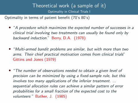
Theoretical work (a sample of it)Optimality in Clinical Trials I

Optimality in terms of patient benefit (70’s 80’s)

• “A procedure which maximizes the expected number of successes in aclinical trial involving two treatments can usually be found only bybackward induction.” Berry, D.A. (1978)

• “Multi-armed bandit problems are similar, but with more than twoarms. Their chief practical motivation comes from clinical trials”Gittins and Jones (1979)

• “The number of observations needed to obtain a given level ofprecision can be minimized by using a fixed-sample rule, but thisinvolves too many applications of the inferior treatment. ...sequential allocation rules can achieve a similar pattern of errorprobabilities for a small fraction of the expected cost to thevolunteers ” Bather, J. (1985)

Theoretical work (a sample of it)Optimality in Clinical Trials II

Optimality in terms of patient benefit (from 2000’s and from the 30’s!)

• The optimal sample size of a 2-armed RCT (optimal in terms ofpatient benefit) is ∝ the square root of the size of the total patientpopulation (

√N). Cheng et al (2003)

• Suggested to randomise patients with a probability ∝ the posteriorprobability of an arm being superior than the other. “This would beimportant in cases where either the rate of accumulation of data isslow or the individuals treated are valuable, or both. ”Thompson, W. (1933)

Optimality in Clinical Trials IIITheory and Practice

Armitage (1985):

“Yet most of the theoretical work done in this tradition, over the last 20years or so, has found no application whatsoever in the actual conduct oftrials. This lack of contact between theory and practice seems tome quite deplorable. Either the theoreticians have got hold of the wrongproblem, or the practising triallists have shown a culpable lack ofawareness of relevant theoretical developments, or both. In any case, thesituation does not reflect particularly well on the statistical community”

Outline





Discussion

The Curse of DimensionalityMABP and Computational Feasibility

• Solution to the MABP according to Bellman’s principle of optimalityexists but is computationally expensive. Prohibitively so for mostrealistic scenarios.

• The curse of dimensionality was (till early 80’s) the single mostimportant limitation to its applicability in practice (in any context).

Armitage (1985):

“The problem can now be seen as essentially the ’two-armed bandit’problem for a finite horizon. The solution to this can in principle beobtained by dynamic programming methods, but in practice thecomputation involved is prohibitive except for trivially small horizons.”

The Gittins Index: Divide and Conquer!Classic MABP & Infinite Horizon Case

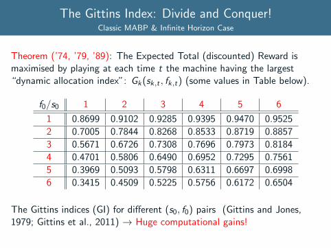
Theorem (’74, ’79, ’89): The Expected Total (discounted) Reward ismaximised by playing at each time t the machine having the largest“dynamic allocation index”: Gk(sk,t , fk,t) (some values in Table below).

f0/s0 1 2 3 4 5 6

1 0.8699 0.9102 0.9285 0.9395 0.9470 0.9525

2 0.7005 0.7844 0.8268 0.8533 0.8719 0.8857

3 0.5671 0.6726 0.7308 0.7696 0.7973 0.8184

4 0.4701 0.5806 0.6490 0.6952 0.7295 0.7561

5 0.3969 0.5093 0.5798 0.6311 0.6697 0.6998

6 0.3415 0.4509 0.5225 0.5756 0.6172 0.6504

The Gittins indices (GI) for different (s0, f0) pairs (Gittins and Jones,1979; Gittins et al., 2011) → Huge computational gains!

The Gittins index for a clinical trialAn example of the index rule in practice

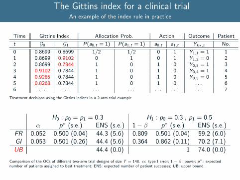
Time Gittins Index Allocation Prob. Action Outcome Patient

t G0 G1 P(a0,t = 1) P(a1,t = 1) a0,t a1,t Yk∗,t No.

0 0.8699 0.8699 1/2 1/2 0 1 Y1,1 = 1 11 0.8699 0.9102 0 1 0 1 Y1,2 = 0 22 0.8699 0.7844 1 0 1 0 Y0,3 = 1 33 0.9102 0.7844 1 0 1 0 Y0,4 = 1 44 0.9285 0.7844 1 0 1 0 Y0,5 = 0 55 0.8268 0.7844 1 0 1 0 . . . 66 . . . . . . . . . . . . . . . . . . . . . 7

Treatment decisions using the Gittins indices in a 2-arm trial example

H0 : p0 = p1 = 0.3 H1 : p0 = 0.3 , p1 = 0.5α p∗ (s.e.) ENS (s.e.) 1− β p∗ (s.e.) ENS (s.e.)

FR 0.052 0.500 (0.04) 44.3 (5.6) 0.809 0.501 (0.04) 59.2 (6.0)GI 0.053 0.501 (0.26) 44.4 (5.6) 0.364 0.862 (0.11) 70.2 (7.1)UB 44.4 (0.0) 1 74.0 (0.0)

Comparison of the OCs of different two-arm trial designs of size T = 148. α: type I error; 1 − β: power; p∗: expectednumber of patients assigned to best treatment; ENS: expected number of patient successes; UB: upper bound.

The Gittins index for a clinical trialAn example of the index rule in practice

Time Gittins Index Allocation Prob. Action Outcome Patient

t G0 G1 P(a0,t = 1) P(a1,t = 1) a0,t a1,t Yk∗,t No.

0 0.8699 0.8699 1/2 1/2 0 1 Y1,1 = 1 11 0.8699 0.9102 0 1 0 1 Y1,2 = 0 22 0.8699 0.7844 1 0 1 0 Y0,3 = 1 33 0.9102 0.7844 1 0 1 0 Y0,4 = 1 44 0.9285 0.7844 1 0 1 0 Y0,5 = 0 55 0.8268 0.7844 1 0 1 0 . . . 66 . . . . . . . . . . . . . . . . . . . . . 7

Treatment decisions using the Gittins indices in a 2-arm trial example

H0 : p0 = p1 = 0.3 H1 : p0 = 0.3 , p1 = 0.5α p∗ (s.e.) ENS (s.e.) 1− β p∗ (s.e.) ENS (s.e.)

FR 0.052 0.500 (0.04) 44.3 (5.6) 0.809 0.501 (0.04) 59.2 (6.0)GI 0.053 0.501 (0.26) 44.4 (5.6) 0.364 0.862 (0.11) 70.2 (7.1)UB 44.4 (0.0) 1 74.0 (0.0)

Comparison of the OCs of different two-arm trial designs of size T = 148. α: type I error; 1 − β: power; p∗: expectednumber of patients assigned to best treatment; ENS: expected number of patient successes; UB: upper bound.

The Gittins Index for a Clinical TrialBeyond the Computational Limitation...

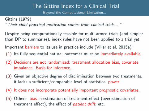
Gittins (1979)“Their chief practical motivation comes from clinical trials... ”

Despite being computationally feasible for multi-armed trials (and simplerthan DP to summarise), index rules have not been applied to a trial yet.

Important barriers to its use in practice include (Villar et al, 2015a):

(1) Its fully sequential nature: outcomes must be immediately available.

(2) Decisions are not randomized: treatment allocation bias, covariateimbalance. Basis for inference.

(3) Given an objective degree of discrimination between two treatments,it lacks a sufficient/comparable level of statistical power.

(4) It does not incorporate potentially important prognostic covariates.

(5) Others: bias in estimation of treatment effect (overestimation oftreatment effect), the effect of patient drift, etc.

The Gittins Index for a Clinical TrialBeyond the Computational Limitation...

Gittins (1979)“Their chief practical motivation comes from clinical trials... ”

Despite being computationally feasible for multi-armed trials (and simplerthan DP to summarise), index rules have not been applied to a trial yet.

Important barriers to its use in practice include (Villar et al, 2015a):

(1) Its fully sequential nature: outcomes must be immediately available.

(2) Decisions are not randomized: treatment allocation bias, covariateimbalance. Basis for inference.

(3) Given an objective degree of discrimination between two treatments,it lacks a sufficient/comparable level of statistical power.

(4) It does not incorporate potentially important prognostic covariates.

(5) Others: bias in estimation of treatment effect (overestimation oftreatment effect), the effect of patient drift, etc.

Outline





Discussion

The Forward Looking Gittins IndexIntroducing Randomization to the Gittins Index Rule

Assume that T patients are enrolled sequentially in groups of size b overJ stages, so that J × b = T . In Villar et al (2015b) we defined groupallocation probabilities based on the GI as follows:Simplest example: b = 2. Priors: control (s(0,0), f(0,0)) = (1, 2) and experimental (s(1,0), f(1,0)) = (1, 1)

j = 1,G1(1, 1) = 0.8699G0(1, 2) = 0.7005

j = 2,G1(1, 2) = 0.7005G0(1, 2) = 0.7005

12

Y1,0 = 0

j = 2,G1(2, 1) = 0.9102G0(1, 2) = 0.7005

12

Y1,0= 1

What is the (patient-average) probability of each arm being allocated in the next block using the GI (and given the priors)?

π1,0 =(0 × 1) + (0 × 1/2 + 1/2 × 1/2)

2= 1/8 , π1,1 =

(1 × 1) + (1 × 1/2 + 1/2 × 1/2)

2= 7/8.

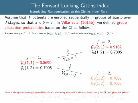
The Forward Looking Gittins IndexIntroducing Randomization to the Gittins Index Rule

Assume that T patients are enrolled sequentially in groups of size b overJ stages, so that J × b = T . In Villar et al (2015b) we defined groupallocation probabilities based on the GI as follows:Simplest example: b = 2. Priors: control (s(0,0), f(0,0)) = (1, 2) and experimental (s(1,0), f(1,0)) = (1, 1)

j = 1,G1(1, 1) = 0.8699G0(1, 2) = 0.7005

j = 2,G1(1, 2) = 0.7005G0(1, 2) = 0.7005

12

Y1,0 = 0

j = 2,G1(2, 1) = 0.9102G0(1, 2) = 0.7005

12

Y1,0= 1

What is the (patient-average) probability of each arm being allocated in the next block using the GI (and given the priors)?

π1,0 =(0 × 1) + (0 × 1/2 + 1/2 × 1/2)

2= 1/8 , π1,1 =

(1 × 1) + (1 × 1/2 + 1/2 × 1/2)

2= 7/8.

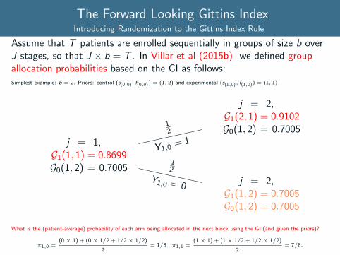
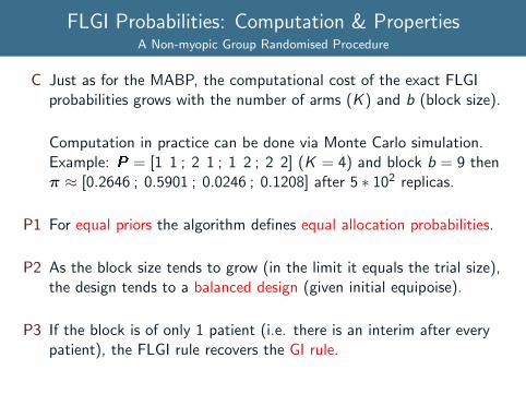
FLGI Probabilities: Computation & PropertiesA Non-myopic Group Randomised Procedure

C Just as for the MABP, the computational cost of the exact FLGIprobabilities grows with the number of arms (K ) and b (block size).

Computation in practice can be done via Monte Carlo simulation.Example: P = [1 1 ; 2 1 ; 1 2 ; 2 2] (K = 4) and block b = 9 thenπ ≈ [0.2646 ; 0.5901 ; 0.0246 ; 0.1208] after 5 ∗ 102 replicas.

P1 For equal priors the algorithm defines equal allocation probabilities.

P2 As the block size tends to grow (in the limit it equals the trial size),the design tends to a balanced design (given initial equipoise).

P3 If the block is of only 1 patient (i.e. there is an interim after everypatient), the FLGI rule recovers the GI rule.

Outline





Discussion

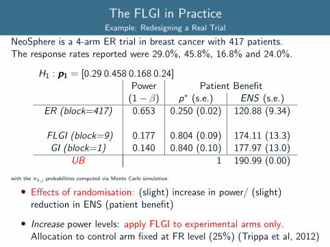
The FLGI in PracticeExample: Redesigning a Real Trial

NeoSphere is a 4-arm ER trial in breast cancer with 417 patients.The response rates reported were 29.0%, 45.8%, 16.8% and 24.0%.

H1 : p1 = [0.29 0.458 0.168 0.24]Power Patient Benefit

(1− β) p∗ (s.e.) ENS (s.e.)

ER (block=417) 0.653 0.250 (0.02) 120.88 (9.34)

FLGI (block=9) 0.177 0.804 (0.09) 174.11 (13.3)GI (block=1) 0.140 0.840 (0.10) 177.97 (13.0)

UB 1 190.99 (0.00)

with the πk,j probabilities computed via Monte Carlo simulation.

• Effects of randomisation: (slight) increase in power/ (slight)reduction in ENS (patient benefit)

• Increase power levels: apply FLGI to experimental arms only.Allocation to control arm fixed at FR level (25%) (Trippa et al, 2012)

The FLGI in PracticeExample: Redesigning a Real Trial

NeoSphere is a 4-arm ER trial in breast cancer with 417 patients.The response rates reported were 29.0%, 45.8%, 16.8% and 24.0%.

H1 : p1 = [0.29 0.458 0.168 0.24]Power Patient Benefit

(1− β) p∗ (s.e.) ENS (s.e.)

ER (block=417) 0.653 0.250 (0.02) 120.88 (9.34)C FLGI (block=9) 0.816 0.665 (0.06) 166.40 (11.9)

FLGI (block=9) 0.177 0.804 (0.09) 174.11 (13.3)GI (block=1) 0.140 0.840 (0.10) 177.97 (13.0)

UB 1 190.99 (0.00)

with the πk,j probabilities computed via Monte Carlo simulation.

• Effects of randomisation: (slight) increase in power/ (slight)reduction in ENS (patient benefit)

• Increase power levels: apply FLGI to experimental arms only.Allocation to control arm fixed at FR level (25%) (Trippa et al, 2012)

Outline





Discussion

Tailoring Treatment to Patients’ CharacteristicsThe Personalised Medicine & Big Data Challenge

• FDA has recently approved several cancer drugs for use in patientswhose tumours have specific genetic characteristics.

• This has strengthened the promise of“personalised medicine”- thetailoring of treatment to the individual characteristics of each patient.

How can trials find treatments that work for a subgroup of patients?

• The challenge is on how to do so in contexts in which there areseveral promising treatments and relatively few patients to test them- even fewer if a treatment works only within a subgroup.

• Some recent trials have used covariate-adjusted response-adaptive(CARA) randomisation (Rosenberger et al, 2001) to more quicklyidentify superior treatments among several, mainly treatments thatwork better within subgroups. E.g., I-SPY II or BATTLE trial.

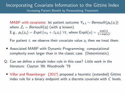
Incorporating Covariate Information to the Gittins IndexIncreasing Patient Benefit by Personalising Treatment

MABP with covariates: let patient outcome Yk,t ∼ Bernoulli(pk(zt))where Zt ∼ Bernoulli(q) (with q known).

E.g., pk(zn) = Expit (αk + βkzt) ∀t, where Expit(u) = exp(u)1+exp(u) .

For patient t, we observe their covariate value zt then we treat them.

• Associated MABP with Dynamic Programming: computationalcomplexity even larger than in the classic case. (Deterministic)

Q: Can we define a simple index rule in this case? Little work in theliterature: Clayton ’89; Woodroofe ’79

• Villar and Rosenberger (2017) proposed a heuristic (extended) Gittinsindex rule for a binary endpoint with a discrete covariate with C levels.

The MABP with covariates and the CARA FLGISummary of how the non-myopic CARA procedure is derived

(1) We consider a MABP with K experimental arms, a control arm andT patients. Before arm k is allocated to patient t, a binary covariateZt is observed. Immediately after, a binary response Yt,n is observed.

(2) Reformulate the above MABP: for every treatment-covariatecombination there exists a combination arm kz . E.g., the arm “00”corresponds to the control arm and covariate negative patients.

New reformulated MABP has 2 (K + 1) combinations arms (with ratepkt) and patients are optimally allocated to arms with the constraintthat they are only allowed arms feasible given their biomarker profile.

(3) We defined a modified GI rule: each patient gets the treatment withthe highest GI among the arms available for their biomarker profile.

(4) From this modified GI, a randomised group allocation procedure isdefined as in Villar et al (2015b) but for every covariate value (andblock) we have a different vector of allocation probabilities πk,j(Z ).

The CARA FLGI in PracticeSimulation Results

3-arm trial 300 patients pk0 = (0.22; 0.34; 0.49), pk,1 = (0.47; 0.71; 0.37).Treatment-covariate interaction: best arm for covariate negative patientsis arm 2 while for covariate positive patients is arm 1.

Power Patient Benefit(1− β0) (1− β1) p∗0 (s.d) p∗1 (s.d) ENS (s.d)

ER (b=300) 0.82 0.63 0.33 (0.04) 0.33 (0.04) 130.71 (9.3)CARA CFLGI (b=10) 0.85 0.79 0.55 (0.16) 0.62 (0.06) 148.36 (9.6)

CARA FLGI (b=10) 0.13 0.03 0.75 (0.22) 0.86 (0.16) 166.73 (11.2)CARA GI (b=1) 0.11 0.03 0.78 (0.24) 0.88 (0.18) 169.39 (11.4)

CARA FLGI probabilities (Monte Carlo simulation), T = 300, pz = 0.5 and 5000 runs.

• Treatment-covariate interactions are detected by the CARA(Covariate-Adjusted Response Adaptive) FLGI procedure but itsstatistical power is very low.

• In a multi-armed case the CARA CFLGI addresses the powerlimitation (though in a two-arm setting power may be insufficient).

Outline





Discussion

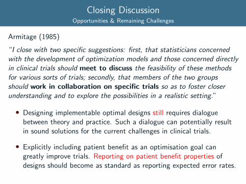
Closing DiscussionOpportunities & Remaining Challenges

Armitage (1985)

“I close with two specific suggestions: first, that statisticians concernedwith the development of optimization models and those concerned directlyin clinical trials should meet to discuss the feasibility of these methodsfor various sorts of trials; secondly, that members of the two groupsshould work in collaboration on specific trials so as to foster closerunderstanding and to explore the possibilities in a realistic setting.”

• Designing implementable optimal designs still requires dialoguebetween theory and practice. Such a dialogue can potentially resultin sound solutions for the current challenges in clinical trials.

• Explicitly including patient benefit as an optimisation goal cangreatly improve trials. Reporting on patient benefit properties ofdesigns should become as standard as reporting expected error rates.

References IQuestions & Comments

Armitage, P. The search for optimality in clinical trials. International Statistical Review:15-24, 1985.

Berry, Donald A Modified two-armed bandit strategies for certain clinical trials Journalof the American Statistical Association: 73(362) 339–345, 1978.

Gittins, J. and Jones, D. A dynamic allocation index for the discounted multiarmedbandit problem. Biometrika, 66(3):561–565, 1979.

Bather, J.A. On the allocation of treatments in sequential medical trials InternationalStatistical Review/Revue Internationale de Statistique,1–13, 1985.

Cheng, Yi and Su, Fusheng and Berry, Donald A Choosing sample size for a clinical trialusing decision analysis Multi-armed bandit allocation indices, 90(4) 923–936, 2003.

Gittins, J. and Glazebrook, K. and Weber, R. Multi-armed bandit allocation indices.Wiley, 2011.

Thompson, W. R. On the likelihood that one unknown probability exceeds another inview of the evidence of two samples. Biometrika 25(3/4) 285–294 (1933)

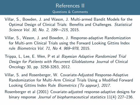
References IIQuestions & Comments

Villar, S., Bowden, J. and Wason, J. Multi-armed Bandit Models for theOptimal Design of Clinical Trials: Benefits and Challenges. StatisticalScience Vol. 30, No. 2, 199—215, 2015.

Villar, S., Wason, J. and Bowden, J. Response-adaptive Randomizationfor Multi-arm Clinical Trials using the Forward Looking Gittins Indexrule Biometrics Vol. 71, No 4. 969–978, 2015.

Trippa, L, Lee, E. Wen, P et al Bayesian Adaptive Randomized TrialDesign for Patients with Recurrent Glioblastoma Journal of ClinicalOncology 30, pp. 3258-3263, 2012.

Villar, S. and Rosenberger, W. Covariate-Adjusted Response-AdaptiveRandomization for Multi-Arm Clinical Trials Using a Modified ForwardLooking Gittins Index Rule Biometrics (To appear), 2017.

Rosenberger et al (2001) Covariate-adjusted response-adaptive designs forbinary response Journal of biopharmaceutical statistics 11(4) 227–236.

Thank you!

What do we mean by computational infeasibilitySource: Don Berry’s presentations

State space & Dynamic Programming for T=7

Dynamic program-ming for

N = 100 and n = 7:

Today

New stateafter failon arm B

New stateafter succ.on arm B

Use arm B

Use arm A

New stateafter failon arm A

New stateafter succ.on arm A

Earn-learn dilemma and block sizeHow to select block size? Should we ramp up accrual?

0.5 0.6 0.7 0.8 0.9

130

140

150

160

170

180

190

Power

ENS

b = 1b = 5b = 10b = 25b = 50b = 90

FLGI

TS

CFLGI

TP

FR

Documents

From Multi-armed Bandit Problems to Response-Adaptive