From  Mott  Insulating  to  Superfluid  in  

Optical  Lattices  

Phys  569  ESM  Term  Paper  

Shu  Chen    

ABSTRACT  

This  essay  introduces  the  Bose-­‐Hubbard  model  (BHM),  which  describes  the  

behavior  of  bosonic  atoms  in  optical  lattices  with  strong  interactions.  Then  

this  model  is  applied  to  describe  two  phases:  superfluid  and  Mott  insulator.  

The  phase  diagram  and  experiments  concerning  this  are  also  discussed  in  

this  essay.  

 

1. Introduction Since  the  realization  of  Bose-­‐Einstein  condensation  in  ultra  cold  dilute  gases,  atomic  

and  molecular  physics  has  stepped  into  a  whole  new  chapter  [1].  During  the  recent  

decade,  using  atoms  confined  in  optical  lattice  to  simulate  strongly  correlated  

electrons  and  to  explore  the  physics  nature  has  grasped  great  attention.  With  the  

ability  to  tune  interaction  between  atoms  through  Feshbach  resonances  [2],  and  to  

generate  strong  optical  periodic  potential  [3],  we  can  achieve  this  goal.  In  this  essay,  

I  first  develop  Bose-­‐Hubbard  model  (BHM)  describing  ultra-­‐cold  atoms  in  optical  

lattices,  then  two  novel  phases,  superfluid  and  Mott  insulating  phases,  coming  from  

different  limits  are  discussed  based  on  BHM  and  simulations.  Besides,  experimental  

results  are  also  presented.  

 

2.  Theoretical  Approach  1) Bose-Hubbard Model

At the beginning, I’ll first introduce the Hamiltonian operator using spatial operators,

which describes the behavior of bosonic atoms in an optical lattice with external trapping

potential [4],

𝐻 = 𝑑!𝑥  𝜓! 𝑥 −ℏ!

2𝑚 ∇! + 𝑉! 𝒙 + 𝑉! 𝒙 𝜓 𝒙

+  124𝜋𝑎!ℏ!

𝑚 𝑑!𝑥  𝜓! 𝑥  𝜓! 𝑥 𝜓 𝒙 𝜓 𝒙 .

(1)

In this first term, 𝜓 𝒙 is a boson field operator for atoms in a given internal atomic state;

𝑉! 𝒙 is the optical lattice potential; and 𝑉! 𝒙 describes an additional external trapping

potential (varying very slowly over space). As the simplest example, 𝑉!(𝒙) has harmonic

form: 𝑉! 𝑥 = sin! 𝑘𝑥!!!!! with wave vector 𝑘 = 2𝜋/𝜆 and 𝜆 the wavelength of laser

light. This harmonic lattice has a period of 𝑎 = 𝜆/2. The magnitude of 𝑉!, which is

induced by the Stark effect of interfering laser beams, is related to the polarizability of

dynamic atoms times the laser intensity.

The second term of the Hamiltonian approximates the interaction between bosonic atoms

by a short-range pseudo-potential with 𝑎! the s-wave scattering length and m the mass of

the atoms.

Obviously, this “bosonic” Hamiltonian has the same form with that describing electrons

in solid, so they should have the same set of solutions. Therefore, the energy eigenstates

are Bloch wave functions. To move forward, we can transform these Bloch wave states to

a set of Wannier functions, which are well localized on each site.

Then we can expand field operator 𝜓 𝑥 in Wannier basis and only keep the lowest

vibrational states, 𝜓 𝑥 = 𝑏!𝑤 𝑥 − 𝑥!! . An important assumption here is that the

energies involved in the system dynamics are small compared to excitation energies to

the first excited band. We will then obtain the Bose-Hubbard model (BHM) Hamiltonian

𝐻 = −𝐽 𝑏!!𝑏!!!,!!

+ 𝜖!𝑛!!

+12𝑈 𝑛! 𝑛! − 1

!

,

(2)

where the operators 𝑛! = 𝑏!!𝑏! represent the number of bosonic atoms at lattice site 𝑖; the

annihilation and creation operators 𝑏! and 𝑏!! obey the canonical commutation relations

𝑏! , 𝑏!! = 𝛿!". The parameters U corresponds to the strength of the on site repulsion of

two atoms on a same lattice site; J is hopping matrix element between nearest neighbor

sites 𝑖, 𝑗; 𝜖! is related to the trapping potential.

Fig.  1.  (a)  BHM  in  an  optical  lattice.  Flat  bottom  curve  is  the  external  trapping  potential.  (b)  Relation  between  𝑈𝑎/𝐸!𝑎!  and  well  depth  𝑉!.  

Before moving on, let us recall the Hubbard model for electrons (fermions).

2) Hubbard Model for Fermions

This model is well known as a paradigm of strong electron correlation in condensed

matter [5],

𝐻 = −𝑡 𝑎!"! 𝑎!"!!"!

+ 𝑈 𝑛!↑𝑛!↓!

,

(3)

where 𝑡 is the hopping term, and 𝑈 represents the on-site interaction.

Besides the dimensionality, the behavior of this Hubbard Hamiltonian is characterized by

three dimensionless parameters: the ratio of Coulomb interaction to the bandwidth 𝑈/𝑡,

average number of electrons per site 𝑛, and the temperature 𝑇/𝑡.

Let us consider a special case, half-filled system 𝑛 = 1 under zero temperature. In the

limit 𝑈/𝑡 ≪ 1, the interaction is weak, the Hamiltonian turns to 𝐻 = −𝑡∑𝑎!"! 𝑎!".

Therefore we can expect that electrons could hop freely from one site to another to gain

kinetic energy. In this case, this model describes a weakly interacting electron system. In

the opposite limit 𝑈/𝑡 ≫ 1, hopping is inhibited between sites, so filling number 𝑛 = 1 is

“pinned” on each site and this makes a special insulator called Mott insulator.

3) Superfluid Phase in Optical Lattices

Now, we come back to Mott-Hubbard model. When 𝑈 = 0, just like I mention in the

second section, the BHM Hamiltonian 𝐻 = −𝐽∑𝑏!!𝑏! = ∑𝜖!𝑎!!𝑎!. All N atoms stay in

the ground state, which is 𝒌 = 0 Bloch state of the lowest band. In a lattice with 𝑁! sites,

at zero temperature, this state could be written as [1]

|𝛹! 𝑈 = 0 =1𝑁!𝑎!!!! !|0 =

1𝑁!

1𝑁!

𝑏!!

!

!

|0 .

(4)

The simplest excitation state is

𝛹 = 𝑎!! 𝛹! 𝑈 = 0 .

(5)

When 𝑈 is non-zero, in the limit of 𝑈/𝑡 ≪ 1, (1) can be reduced to a Gross-Pitaevskii

equation

𝐻 = −ℏ!

2𝑚 ∇! + 𝑉! 𝒙 + 𝑉! 𝒙 +4𝜋𝑎!ℏ!

𝑚 𝜓 𝒙 !

(6)

Then, the ground state is the Gross-Pitaevskii-type superfluid with a condensate fraction,

which is equal to 1.

If the filling number 𝑁/𝑁! is not an integer, but a finite number, the ground state can be

written in coherent state form [1]

exp 𝑁𝑎!!!! |0 = exp𝑁𝑁!𝑏!!  |0 !

!

.

(7)

From the left side, we can see that the average total atom number is N (all with 𝒌 = 0).

The right side means that there are 𝑛 = 𝑁/𝑁! atoms at each site. We can expand the

exponential operator on each site (I assume 𝑁/𝑁_𝐿   = 1 here)

exp𝑁𝑁!𝑏!! = 1+ 𝑏!! +

12! 𝑏!

!! +13! 𝑏!

!! +⋯.

(8)

The probability that there are more than one particle on each site is (𝑒 − 1− 1)/𝑒 = 1−

2/𝑒 = 0.27. So if 𝑈/𝑡 were finite, this state would not be energetic favorable, which will

lead to the next state: Mott insulating phase.

4) Mott Insulating Phase in Optical Lattices

In the limit 𝑈/𝑡 ≫ 1, with unit filling number (𝑁 = 𝑁!), compared to the case for

fermions, hopping of atoms between sites is negligible, so the ground state is [1]

|𝛹!!!! 𝐽 = 0 = 𝑏!!

!

 |0  .

(6)

This is just a simple product of local Fock states with precisely one atom per site.

In fact, there is a very interesting calculation result [6] to demonstrate this state in

𝑈/𝑡 ≫ 1 regime. These results calculated the entropy vs. temperature figure of bosonic

atoms on a cubic optical lattice with 𝑁! ≈ 3×10! sites.

It should be noted that the well depth V is related to bosons interaction term parameter U

as,

𝑈𝐽 ~

𝑎𝑑 exp 2

𝑉!𝐸!

, 𝐸! ≡ℏ!

2𝑚 𝑘!.

Therefore, 𝑉! = 20𝐸! means 𝑈/𝐽 ≫ 1, which should be Mott insulating regime.

 

Fig. 2. Entropy vs. temperature curves for 𝑁! ≈ 3×10! site cubic lattice, with filling fact n=1 (left) and n=4 (right). The well depth varies from V=0 to 20𝐸! (with a spacing of 2𝐸! between each curve). The entropy plateau 𝑆! is shown as a dashed line in each graph.

Now, I assume at low temperature, the 𝑉! = 20𝐸! curve represents Mott insulating phase

and calculated entropy plateau in a simple way.

Then the simplified problem is what is the entropy of 𝑁! = 𝑛𝑁! bosons occupying 𝑁!

sites at temperature T.

𝑆 = 𝑘!𝑇 log𝛺 ,      𝛺 =𝑁! + 𝑁! − 1 !𝑁!! 𝑁! − 1 !

Apply Stirling’s approximation,

𝑆𝑘!𝑇

≈ 𝑁! log𝑁! + 𝑁!𝑁!

+ 𝑁! log𝑁! + 𝑁!𝑁!

= 𝑁! 𝑛 log𝑛 + 1𝑛 + log 𝑛 + 1 .

So for 𝑛 = 1, !!!!

= 2 log 2𝑁! = 4.13×10!; for n=4, !!!!

= log 5+ 4 log !!𝑁! =

7.45×10!.

These two results both coincide with Fig. 2.

3. Phase Diagram and Experimental Demonstration

The zero-temperature phase diagram of BHM is shown in Fig. 3(a). In this graph,

normalized chemical potential denotes roughly the local density of atoms. At a given

chemical potential, the phase is a function of the ratio of hopping and on-site interaction

𝐽/𝑈. In fact the chemical potential is a spatially slowly varying function, 𝜇! = 𝜇! − 𝜖!

with 𝜖! = 0 at the trap center. While at the boundary of the trap, 𝜇! vanishes. Fig. 3(b)

assumes that 𝜇! falls into filling number 𝑛 = 2 “Mott lobe”. One obtains series of Mott

insulating phases and superfluid phases from the center to trap boundary [1]. Therefore,

the density profile is like a wedding-cake.

It should be noted that, the compressibility 𝜅 = 𝜕𝑛/𝜕𝜇 equals to zero in Mott insulating

(MI) phase because n stays as a constant, which means that MI states are incompressible.

This very novel density profile is demonstrated numerically and experimentally as shown

in Fig. 4 [7] and Fig. 5 [8].

Fig. 3. (a) zero-temperature phase diagram of BHM. (b) Corresponding real space figure. [1]

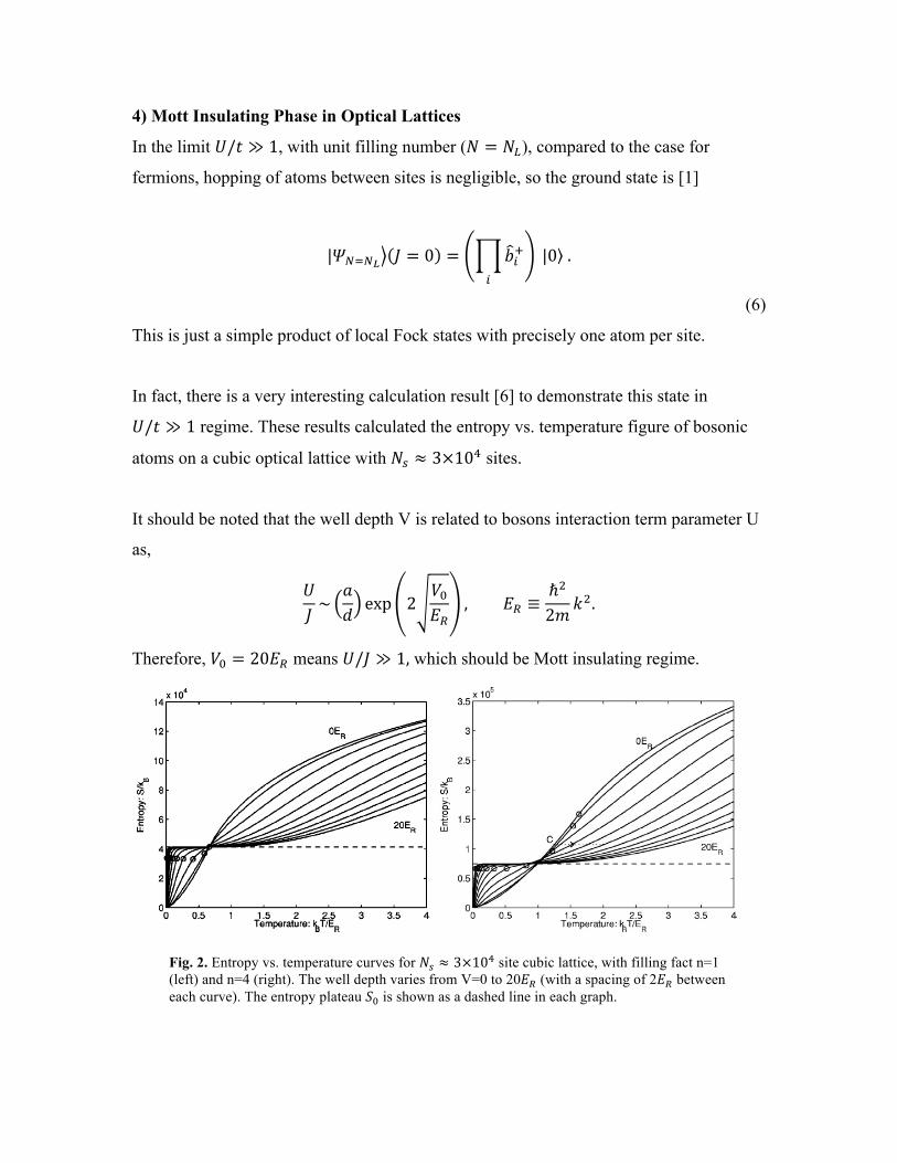
Fig. 4. Monte-Carlo results of local density vs. position relation of a 2D confined bosonic atoms system. The lattice depth of b) is stronger than that of a). a) U/t=6.7 b) U/t=25.

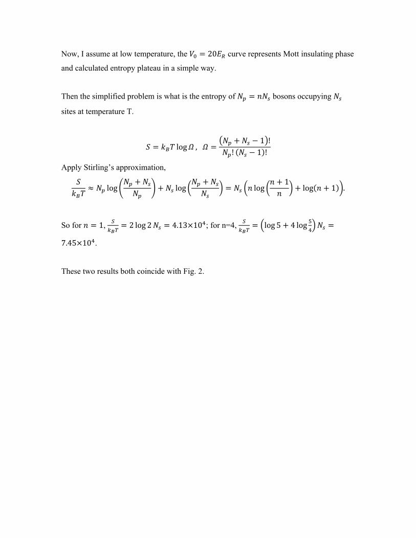
Fig. 5. Integrated distribution of (a) a

superfluid and (b) a Mott insulating

state of bosonic atoms in a harmonic

trapped optical lattice. Grey solid line

represents the total density profile over

z-direction. Blue and red are for singly

and doubly occupied sites. It is shown

that the n=1 blue dashed line has a

plateau through the core n=2 region in

z-direction. Therefore this graph

indirectly proves the wedding-cake-

like density profile.

4. Conclusion In this essay, I introduced Bose-Hubbard model and two novel phases coming from this. I

also showed the numerical and experimental evidence to support this model. The

realization of Hubbard model gives us another perspective to investigate strongly

interacting condensed systems, which is very meaningful.

Reference:

[1] I. Bloch, J. Dalibard, and W. Zwerger, “Many-body physics with ultracold gases”,

Rev. Mod. Phy. 80, 885-964 (2008).

[2] P. Courteille, R. Freeland, D. Heinzen, F. van Abeelen, and B. Verhaar, Phys. Rev.

Lett. 81, 69 (1998).

[3] Greiner, M., M. O. Mandel, T. Esslinger, T. Hänsch, and I. Bloch, Nature 415, 39

(2002a).

[4] D. Jaksch, C. Bruder, J. I. Cirac, C. W. Gardiner, and P. Zoller, “Cold Bosonic Atoms

in Optical Lattices”, Phys. Rev. Lett. 81, 3108 (1998).

[5] A. Altland and B. Simons, “Condensed Matter Field Theory”, Cambridge, (2010)

[6] P. B. Blakie and J. V. Porto, “Adiabatic loading of bosons into optical lattices”, Phys.

Rev. A 69, 013603 (2004)

[7] Wessel, S., F. Alet, M. Troyer, and G. G. Batrouni, Phys. Rev. A 70, 053615 (2004).

[8] Fölling, S., A. Widera, T. Müller, F. Gerbier, and I. Bloch, Phys. Rev. Lett. 97,

060403 (2006).