From Local to Global: Offshoring and Asset

Prices ∗

Lorenzo Bretscher

LSE†

JOB MARKET PAPER

Abstract

Industries differ in the extent to which they can offshore their production. I documentthat industries with low offshoring potential have 7.31% lower stock returns per yearcompared to industries with high offshoring potential, suggesting that the possibilityto offshore affects industry risk. This risk premium is concentrated in manufacturingindustries that are exposed to foreign import competition. Put differently, the optionto offshore effectively serves as insurance against import competition. A two-countrygeneral equilibrium dynamic trade model in which firms have the option to offshorerationalizes the return patterns uncovered in the data: industries with low offshoringpotential carry a risk premium that is increasing in foreign import penetration. Withinthe model, the offshoring channel is economically important and lowers industry riskup to one-third. I find that an increase in trade barriers is associated with a drop inasset prices of model firms. The model thus suggests that the loss in benefits fromoffshoring outweighs the benefits from lower import competition. Importantly, themodel prediction that offshorability is negatively correlated with profit volatility isstrongly supported by the data.

First Version: February 2017

This Version: November 2017

∗I would like to thank Veronica Rappoport, Andrea Vedolin, Ulf Axelsson, Oliver Boguth (discussant), HarrisDellas, Boyan Jovanovic, Ian Martin, Gianmarco Ottaviano, Christopher Polk, Andreas Rapp (discussant), AlirezaTahbaz-Salehi, Andrea Tamoni, Branko Urosevic, Philip Valta, Alexandre Ziegler (discussant) and, especially,Christian Julliard and Lukas Schmid as well as the seminar participants at LSE, the University of Bern, the SwissEconomists Abroad Conference, the Belgrade Young Economist Conference, the Doctoral Tutorial of the EuropeanFinance Association and the HEC Paris Finance PhD Workshop for valuable comments. I also thank J. BradfordJensen for sharing his data on industry tradability. All remaining errors are my own.

†Department of Finance, Email: l.p.bretscher@lse.ac.uk

1 Introduction

“The typical ‘Made in’ labels in manufactured goods have become archaic symbols of an old

era. These days, most goods are ‘Made in the World’.” Antras (2015)

Over the recent decades, the world economy has seen a gradual dispersion of the production process

across borders. Firms increasingly organize their production on a global scale and choose to offshore

parts, components, or services to producers in foreign countries. The revolution in information and

communication technology (ICT) and the dismantling of trade barriers allow firms to engage in global

production networks, or global sourcing strategies, in order to cut costs.1 For this reason, the choice

of production location is a potentially valuable decision tool at the firm level. However, firms/industries

differ in their ability to engage in offshoring due to the nature of their products and tasks involved in the

production process. In short, in the era of globalization, the possibility to take a business from local to

global has heterogenous implications for the cross-section of industries.

In this paper, I exploit cross-sectional heterogeneity in the ability to offshore to study how the possibil-

ity to relocate the production process affects industries’ cost of capital. In particular, I focus on industries’

ability to offshore the employed labor force and examine whether this is reflected in the cross-section of

returns.2 To this end, I construct a measure of labor offshorability at the industry level. The measure is

calculated in two steps. In the first step, using data from the O*NET program of the U.S. Department of

Labor, I calculate an offshorability score at the occupation level, as in Acemoglu and Autor (2011).3 In

the second step, I aggregate occupation offshorability scores by industry, weighting them by the product of

employment and the wage bill associated with each occupation. The resulting data set covers an average

of 331 industries per year during the period 1990 to 2016.4

I sort industries in five offshorability quintiles and find that the strategy that is long the low and short

the high offshorability quintile portfolios, L-H, yields average annual excess returns of 7.31 percent and a

Sharpe ratio of 0.48. This premium is not spanned by well-known risk factors such as Fama and French

(2015) and Carhart (1997). Even after controlling for the five factors of Fama and French (2015), L-H

generates positive average annual excess returns of 4.18 percent.

1 In addition to the ICT revolution and lower trade barriers, political developments have led to an increase inthe fraction of world population that actively participates in the process of globalization (Antras (2015)).

2 In a related paper, Donangelo (2014) shows that industries that employ many workers with transferable skillsare more exposed to aggregate shocks.

3 A strand of literature in labor economics studies offshoring of tasks at the occupation level. See, for example,Jensen and Kletzer (2010), Goos and Manning (2007), Goos, Manning, and Salomons (2010), Acemoglu and Autor(2011), and Firpo, Fortin, and Lemieux (2013).

4 Industries are defined at the three-digit Standard Industry Classification (SIC) from 1990 to 2001 and at thefour-digit North American Industry Classification System (NAICS) level thereafter.

1

Furthermore, I split the sample into manufacturing and service industries. In univariate sorts, the L-H

excess return spread in manufacturing is two to three times larger in magnitude compared to services.

Moreover, for service industries, the premium is explained by the CAPM and a positive loading on the

market. For manufacturing industries, on the other hand, common linear factor models fail to explain

the returns generated by L-H. Consistent with this, in annual panel regressions at the firm level, I find

that lagged industry offshorability significantly predicts annual excess returns for manufacturing but not

for service industries. The results for manufacturing firms are economically meaningful: a one standard

deviation increase in offshorability is associated with 4% to 5% lower annual excess stock returns. These

results are robust to controlling for firm characteristics known to predict excess returns.

A first-order question is what drives the heterogeneity between manufacturing and services. A poten-

tial explanation is based on the degree of foreign import competition. While manufacturing industries

have seen a sharp increase in foreign competition, mainly from low-wage countries, this is not the case

for service industries.5 I relate my results to foreign import competition in manufacturing industries

using conditional double sorts of excess returns on proxies of import competition and offshorability. I

find that the L-H premium is monotonically increasing in import competition.6 The results are robust to

different proxies of import competition: First, I use a direct measure of import penetration from low-wage

countries defined as the imports from low-wage countries divided by the sum of domestic production and

net exports in a given industry (see Bernard, Jensen, and Schott (2006a)). Second, I use industry-specific

shipping costs as a proxy for barriers to trade.7 These results are consistent with the U.S. having a

comparative advantage in providing services but not in manufacturing (see also Jensen (2011)).8

In a related paper, Barrot, Loualiche, and Sauvagnat (2017) focus on manufacturing industries and

document that industries more exposed to foreign competition have higher excess returns. While their

work establishes that import competition poses risks for an industry, my findings document that offshoring

allows industries to hedge these risks. Intuitively, being able to offshore allows firms to fight import

competition from low-wage countries by reducing costs through relocating production. Consistent with

this argument, a recent paper by Magyari (2017) shows that offshoring enables U.S. firms to reduce costs

and outperform peers that cannot offshore.

5 This can be seen from U.S. trade balances. While the trade balance in goods is negative and has decreasedsharply over the last 25 years, the trade balance for services is positive and has been stable over time.

6 In line with this, many recent empirical studies, such as Autor, Dorn, and Hanson (2013, 2016) and Pierce andSchott (2016), stress the importance of imports from low-wage countries for understanding the dynamics in U.S.manufacturing industries.

7 Shipping costs are calculated as the markup of the Cost-Insurance-Freight value over the Free-on-Board value,as in Bernard, Jensen, and Schott (2006b).

8 The principle of comparative advantage was first elaborated by Ricardo (1821) and formalized by Heckscher(1919) and Ohlin (1933). They argue that countries have a comparative advantage in activities that are intensivein the use of factors that are relatively abundant in the country.

2

To further improve understanding of the mechanism, I embed the option to offshore in a two-country

general equilibrium dynamic trade model similar to Ghironi and Melitz (2005) and Barrot, Loualiche, and

Sauvagnat (2017) with multiple industries and aggregate risk. I will refer to the two countries as East

and West. My model departs from previous work by allowing firms to offshore part of the production, as

in Antras and Helpman (2004). Moreover, I assume that the East has a comparative cost advantage over

the West in performing offshorable labor tasks. As a result, offshoring to the East allows Western firms

to reduce production costs and diversify aggregate risks. In addition, firms in both countries can export

and sell their products abroad.

The model successfully matches industry- and trade-related moments and generates return patterns

qualitatively, in line with the data. First, it generates a return spread between low and high offshorability

industries. Second, the spread is increasing in the degree of import penetration. Third, excess returns of

multinational companies are higher than for domestic firms. Fourth, industry excess returns are increasing

in import penetration.

Asset price movements in the model are governed by shocks to aggregate productivity in each of the

two countries. The responses of equilibrium quantities to the two aggregate productivity shocks are related

because quantities react to changes in the ratio of aggregate productivity of the two countries: upon arrival

of a positive (negative) productivity shock in the East (West), more Eastern firms find it profitable to

export, which results in an increase in import penetration and competition in the West. As a result,

Western firms experience losses in market share and lower profits. At the same time, offshoring allows

Western firms to reduce production costs, which renders them more competitive towards new market

entrants. Consequently, industries with a higher offshoring potential have smoother profits and dividends.

Put differently, high (low) offshorability industries are less (more) exposed to aggregate productivity

shocks in the model. This difference in exposure to aggregate risk results in an L-H return spread in

industry excess returns, as observed in the data.

To further validate the model, I test three of its main predictions in the data. First, the model predicts

that profit volatility is decreasing in industry offshorability, which is strongly supported by the data: a

one standard deviation increase in industry offshorability is associated with an up to 19.7% lower profit

volatility for the median firm. Second, the model predicts that the offshorability premium is largest in

industries with more price-sensitive consumers. Conditional double sorts of monthly excess returns on

U.S. trade elasticities from Broda and Weinstein (2006) and offshorability confirm this prediction in the

data: the L-H spread is roughly double in magnitude for industries with high compared to low U.S. trade

elasticities. Finally, within the model, low (high) offshorability industries have high (low) covariance with

consumption. Consistent with this, I find that the strategy that is long low and short high offshorability

3

industries has a positive and significant consumption beta in the data.

To quantify the importance of the offshorability channel in the model, I study industry moments in

absence of offshorable labor tasks. The counterfactual indicates that an industry with no offshorability

exhibits substantially higher risk premia (up to 33% or 3.14 percentage points) and lower equity valuations

(a reduction of up to 17%). Hence, offshoring is an economically important channel in the model.

Finally, within the context of my model, I examine the consequences of a sudden increase in trade

costs on goods shipped from East to West. Alternatively, this could be interpreted as a sudden increase in

trade barriers for all goods imported by the West. Intuitively, higher barriers to trade lead to a decrease in

import penetration in the model, which reduces industry risk. However, an increase in trade barriers also

renders offshoring less valuable, since shipment of intermediate goods becomes more costly. Interestingly,

within the model, the loss in benefits from offshoring outweighs the positive effects from lower import

penetration. As a result, consumption and asset prices in the West fall.

The rest of the paper is organized as follows. After the literature review, section 2 details the data

and discusses the construction of the labor offshorability measure. In section 3, I discuss the empirical

findings. Section 4 presents a theoretical model with a calibration. Finally, section 5 concludes.

Literature Review

This paper relates to four main strands of literature. First, the paper relates to the literature that studies

the interaction between labor and asset prices. Danthine and Donaldson (2002) and Favilukis and Lin

(2016) document that operating leverage induced by rigid wages is a quantitatively important channel in

matching financial moments in general equilibrium models.9 More recently, a growing body of papers

focus on different forms of labor heterogeneity and the cross-section of stock returns.10 In particular,

Zhang (2016) finds a real option channel for firms that have the possibility to substitute routine-task

labor with machines. Moreover, Donangelo (2014) shows that industries with mobile workers are more

exposed to aggregate shocks, since mobile workers can walk away for outside options in bad times, making

it difficult for capital owners to shift risk to workers. This paper contributes to the literature by studying

a new dimension of labor heterogeneity, i.e., whether or not a task can be offshored.

Second, this study relates to the literature on the effects of competition and international trade for

asset pricing. Among others Loualiche (2015), Corhay, Kung, and Schmid (2017) and Bustamante and

9 Gomes, Jermann, and Schmid (2017) investigate the rigidity of nominal debt, which creates long-term leveragethat works in a similar way to operating leverage induced by labor.10 See, among others, Gourio (2007), Ochoa (2013), Eisfeldt and Papanikolaou (2013), Belo, Lin, Li, and Zhao

(2015), Kuehn, Simutin, and Wang (2017), Donangelo, Gourio, Kehrig, and Palacios (2016) and Tuzel and Zhang(2017)

4

Donangelo (2016) show that the risk of entry is priced in the cross-section of expected returns. In a

recent and closely related paper, Barrot, Loualiche, and Sauvagnat (2017) focus on risks associated with

import competition and find that firms more exposed to import competition command a sizeable positive

risk premium. Furthermore, Fillat and Garetto (2015) document that multinational firms exhibit higher

excess returns than purely domestic firms. This is rationalized in a model in which selling abroad is

a source of risk exposure to firms: following a negative shock, multinationals are reluctant to exit the

foreign market because they would forgo the sunk cost they paid to enter. While their model shows how

firms’ revenues relate to risk in multinationals, my paper focuses on the relation between firm risk and

labor costs.

Third, a recent line of research studies the consequences of the surge in international trade over the

last decades at the establishment and firm level. Among others, Autor, Dorn, and Hanson (2013) and

Pierce and Schott (2016) show that U.S. manufacturing establishments more exposed to growing imports

from China in their output markets exhibit a sharper decline in employment relative to the less exposed

ones.11 Other studies use tariff cuts to instrument for import competition and find that it affects firms’

capital structure (Xu (2012) and Valta (2012)) and capital budgeting decisions (Bloom, Draca, and Van

Reenen (2015) and Fresard and Valta (2016)). My paper complements this literature by studying asset

pricing implications instead of firm quantities. I find that offshoring allows firms to allocate resources

more efficiently and lowers risks associated with foreign import competition.12 Therefore, my paper also

contributes to the growing body of empirical trade literature that documents that manufacturing firms

have benefited from offshoring. Hummels, Jørgensen, Munch, and Xiang (2016), Chen and Steinwender

(2016) and Bloom, Draca, and Van Reenen (2015) document that offshoring fosters firms’ productivity

and innovation activity. Magyari (2017) shows that offshoring enables U.S. firms to reduce their costs.

She also finds that firms that are able to offshore actually increase their total firm-level employment both

in manufacturing and headquarter service jobs.13

Fourth, this paper relates to the literature that examines the relationship between firm and plant

organization and performance. Empirically, Atalay, Hortacsu, and Syverson (2013) examine the domestic

sourcing by U.S. plants, and Ramondo, Rappoport, and Ruhl (2016) study foreign sourcing by U.S.

multinational firms. These papers show that firms and plants tend to source a large share of their

material inputs from third-party suppliers. My paper documents how sourcing decisions affect asset prices.

11 See also Autor, Dorn, and Hanson (2016), Acemoglu, Autor, Dorn, Hanson, and Price (2016), Amiti, Dai,Feenstra, and Romalis (2016).12 Related papers show that firms suffer less from import competition if they have larger cash holdings (Fresard

(2010)) or higher R&D expenses (Hombert and Matray (2017)).13 Compared to other related papers, Magyari (2017) focuses on employment at the firm level rather than at the

establishment level.

5

Theoretically, Antras and Helpman (2004) formulate a model in which firms decide whether to integrate

the production of intermediate inputs or outsource them with incomplete contracts. Both decision can

either take place domestically or abroad. More recently, Antras, Fort, and Tintelnot (2016) develop a

quantifiable multi-country sourcing model in which global sourcing decisions interact through the firm’s

cost function, and Bernard, Jensen, Redding, and Schott (2016) present a theoretical framework that

allows firms to decide simultaneously on the set of production locations, export markets, input sources,

products to export, and inputs to import. In contrast, my model focuses on the interaction of offshoring

and industry risk. To do so, I incorporate the possibility to offshore into a dynamic trade model with

multiple industries, as in Ghironi and Melitz (2005), Chaney (2008) and Barrot, Loualiche, and Sauvagnat

(2017).14

2 Data

In this section, I first outline the data and the method to construct a measure of labor offshorability at

the occupation level and the industry level. Second, I discuss the financial and accounting as well as

international trade data used in the empirical analysis.

2.1 Measuring Labor Offshorability

As a first step, I calculate a measure of offshorability at the occupation level. To do so, I follow the

recent literature in labor economics and use data from the U.S. Department of Labor’s O*NET program

on the task content of occupations.15 , 16 This program classifies occupations according to the Standard

Occupational Classification (SOC) system and has information on 772 different occupations.17 O*NET

contains information about the tools and technology, knowledge, skills, work values, education, experience

and training needed for a given occupation.18 I follow Acemoglu and Autor (2011) and Blinder (2009)

and calculate an offshorability score at the occupation level.

Acemoglu and Autor (2011) argue that an occupation that requires substantial face-to-face interaction

and needs to be carried out on site is unlikely to be offshored. To capture this notion of offshorability,

14 Melitz (2003) and Bernard, Jensen, Eaton, and Kortum (2003) also allow for firm heterogeneity and heteroge-nous gains from trade.15 For papers that rely on the O*NET data base, see, among others, Jensen and Kletzer (2010), Goos and Manning

(2007), Goos, Manning, and Salomons (2010), Firpo, Fortin, and Lemieux (2013), and Acemoglu and Autor (2011).16 I use O*NET 20.3, available from https://www.onetonline.org/17 Some of the 772 occupations are further detailed into narrower occupation definitions. The total number of

more-detailed occupations in O*NET is 954.18 The O*NET content model organizes these data into six broad categories: worker characteristics, worker

requirements, experience requirements, occupational requirements, labor market characteristics, and occupation-specific information.

6

they focus on seven individual occupational characteristics, which are tabulated in Panel A of table

1. Compared with alternative occupation offshorability scores (see Firpo, Fortin, and Lemieux (2013),

for example), Acemoglu and Autor (2011) base their calculations on fewer occupation characteristics to

mitigate a high correlation with the routine-task content of an occupation.19

[Insert Table 1 here.]

The O*NET database organizes characteristics in work activities or work context (see column 3 of Panel

A in table 1). For work activities, O*NET provides information on “importance” and “level”. I follow

Blinder (2009) and assign a Cobb-Douglas weight of two-thirds to “importance” and one-third to “level”

to calculate a weighted sum for work activities.20 Since there is no “importance” score for work context

characteristics, I simply multiply the relative frequency by the level.21 Thus, the offshorability score for

occupation j, offj, is defined as

offj =1

∑Al=1 I

23jl × L

13jl +

∑Cm=1 Fjm × Ljm

(1)

where A is the number of work activities, Ijl is the importance and Ljl is the level of a given work activity

in occupation j, C is the number of work context elements, Fjm is the frequency and Ljm is the level of

a given work context in occupation j.22 Finally, I take the inverse to obtain a score that is increasing in

an occupation’s offshorability.23

In a second step, I aggregate the occupation offshorability scores at the industry level using industry-

level occupation data from the Occupational Employment Statistics (OES) program of the BLS. This

data set contains information on the number of employees in a given occupation, industry and year. The

data set is based on surveys that track employment across occupations and industries in approximately

200,000 establishments every six months over three-year cycles, representing roughly 62% of non-farm

employment in the U.S. Each industry in the sample was surveyed every three years until 1995 and every

year from 1997 onwards. For the period before 1997, I follow Donangelo (2014) and use the same industry

19 As a robustness check, I also calculate occupation offshorability according to Firpo, Fortin, and Lemieux (2013).They base their calculations on 16 different occupation characteristics, which are organized into three categories:face-to-face contact, on-site and decision-making. The characteristics are tabulated in an online appendix. Theresults of the paper remain qualitatively the same when the measure of Firpo, Fortin, and Lemieux (2013) isemployed and are available upon request.20 The results are robust to different Cobb-Douglas weights. For example, taking simple averages between impor-

tance and level scores does not change any of the results in the paper.21 For example, the level of the work context element “frequency of decision-making” is a number between one

and five: 1 = never; 2 = once a year or more but not every month; 3 = once a month or more but not every week;4 = once a week or more but not every day; or 5 = every day.22 Note that importance and level scores are all rescaled to be between zero and one. Relative frequencies Fjm

lie, by definition, between zero and one.23 The occupation offshorability for Acemoglu and Autor (2011) ranges between one-sixth and one.

7

data for three consecutive years to ensure continuous coverage of the full set of industries. For example,

the data used in 1992 combine survey information from 1990, 1991, and 1992. Unfortunately, the OES

did not conduct a survey in 1996. To avoid a gap, I follow Ochoa (2013) and Donangelo (2014) and rely

on survey information from the years 1993, 1994, and 1995.

The data set employs the OES taxonomy with 258 broad occupation definitions before 1999, the

2000 Standard Occupational Classification (SOC) system with 444 broad occupations between 1999 and

2009, and the 2010 SOC afterwards. To merge the occupation level offshorability with the OES data

set, I bridge different occupational codes using the crosswalk provided by the National Crosswalk Service

Center. Industries are classified using three-digit Standard Industrial Classification (SIC) codes until 2001

and four-digit North American Industry Classification System (NAICS) codes thereafter.24

The OES/BLS data set also includes estimates of wages since 1997. For the 1990 to 1996 period,

I use estimates of wages from the BLS/U.S. Census Current Population Survey (CPS) obtained from

the Integrated Public Use Microdata Series of the Minnesota Population Center.25 I aggregate the

occupation level offshorability measure, offj, by industry, weighting by the wage expense associated with

each occupation:

OFFi,t =∑

j

offj ×empi,j,t × wagei,j,t

∑

j empi,j,t × wagei,j,t(2)

where empi,j,t is the employment in industry i, occupation j and year t, and wagei,j,t measures the annual

wage paid to workers. Using wages at this stage is consistent with placing more weight on occupations

with greater impact on cash flows.26 Lastly, OFFi,t is standardized in each year, i.e., the cross-sectional

mean and standard deviation of the offshorability measure are set to zero and one, respectively. The

resulting data set covers the years 1990 to 2016, with an average of 331 industries.

24 While the OES data set is designed to create detailed cross-sectional employment and wage estimates for theU.S. by industry, because of changes in the occupational classification, it might be challenging to exploit its timeseries variation. For this reason, I focus predominantly on cross-sectional analyses of the data.25 These data are available from https://www.ipums.org/. For more information, see King, Ruggles, Alexander,

Flood, Genadek, Schroeder, Trampe, and Vick (2010)26 I also test for robustness of the empirical analysis by using an industry measure of offshorability that does not

rely on wages, i.e.,

OFF ⋆i,t =

∑

j

offj ×empi,j,t

∑

j empi,j,t.

The results remain qualitatively unchanged and are available upon request.

8

2.2 Financial and Accounting Data

For the empirical analysis, I use monthly stock returns from the Center for Research in Security Prices

(CRSP) and annual accounting information from the CRSP/COMPUSAT Merged Annual Industrial

Files. The sample of firms includes all NYSE-, AMEX-, and NASDAQ-listed securities that are identified

by CRSP as ordinary common shares (with share codes 10 and 11) for the period between January 1990

and December 2016. I follow the literature and exclude regulated (SIC codes between 4900 and 4999)

and financial (SIC codes between 6000 and 6999) firms from the sample. I also exclude observations

with negative or missing sales, book assets and observations with missing industry classification codes.

Firm-level accounting variables are winsorized at the 1% level in every sample year to reduce the influence

of possible outliers. All nominal variables are expressed in year-2009 USD.27 I also use historical segment

data from COMPUSTAT to classify firms in multinationals and domestic firms as in Fillat and Garetto

(2015). Finally, I use COMPUSTAT quarterly to calculate the volatility of sales and profits, as in Minton

and Schrand (1999). A detailed overview of the variable definitions can be found in the online appendix.

2.3 International Trade Data

I use product-level U.S. import and export data for the period 1989 to 2015 from Peter Schott’s website.

For every year, I obtain the value of imports as well as a proxy for shipping costs at the product level that

can be aggregated to the industry level. I follow Hummels (2007) and approximate shipping costs with

freight costs, i.e., the markup of the Cost-Insurance Freight value over Free-on-Board value. Moreover, I

use data on US trade elasticities at the product level from Broda and Weinstein (2006). Finally, data on

U.S. trade balances are from the Bureau of Economic Analysis.

3 Empirical Evidence

In this section, I present the empirical results of the paper. First, I examine the validity of the offshorability

measures. Second, I report that average portfolio excess returns are decreasing in offshorability. Third,

I show that the premium that can be earned by going long low and short high offhsorability industries

is concentrated in manufacturing industries and is not explained by a wide range of linear asset pricing

models. Finally, I offer further empirical evidence that links the offshorability premium to the recent

surge in foreign import competition from low-wage countries.

27 I use the GDP deflator (NIPA table 1.1.9, line 1) and the price index for non-residential private fixed investment(NIPA Table 5.3.4, line 2) to convert nominal into real variables.

9

3.1 Validity and Summary Statistics of Labor Offshorability

I start by examining whether the measures discussed in section 2 deliver reasonable rankings of occupations

and industries in terms of offshorability. Panels B and C of table 1 report the top and bottom ten

occupations by offshorability. Occupations with high offshorability are not restricted with respect to

location or immediacy to the final consumer. Conversely, occupations at the bottom are either closely

related to the location, such as “tree trimming”, or to customers, such as “dentists”. Unfortunately, offj

is, by construction, constant throughout time. Therefore, occupation offshorability is unable to capture

how technological progress has affected the offshorability of individual occupations.28 To the extent that

technological progress has affected offshorability symmetrically across occupations, this is not a concern

for my cross-sectional analysis.

In contrast, industry offshorability inherits some time variation from the changes in the occupation-

industry composition of the U.S. labor force. To gain a better sense of the time-variation in OFFi,t, I

examine the industry rankings for manufacturing and services industries separately.29 Table 2 reports the

top and bottom ten industries by offshoring potential in the years 1992 and 2015 (Panels A and B) and

the transition probabilities (Panel C) between offshorability quintiles for manufacturing industries.30 In

1992, the top industries are predominantly apparel industries, whereas the bottom industries are related

to mining and construction. The 2015 rankings reveal that there is not much variation over time during

the sample period. In fact, even though industries are now classified according to the NAICS system, the

top and bottom ten are similar to 1992.31

Another way to examine the persistence of OFFi,t over time is to look at transition probabilities. I do

so by sorting industries into quintiles of offshorability each year and calculating the transition probabilities

across quintiles. Panel C of table 2 reports the one- and five-year transition probabilities.32 For industries

in the top or bottom quintiles of labor offshorability, the probability of being in the same quintile the

next year (in five years) is close to 90% (80%). For the middle quintiles, the persistence is slightly lower,

approximately 75%, over one year and 60% over five years. To sum up, industry offshorability is very

persistent over time, consistent with offshoring being a slow-moving response to changes in the economic

28 Several authors note that recent technological advances have substantially increased the offshorability of occu-pations. See, among others, Antras (2015) for manufacturing occupations and Jensen (2011) for service industryoccupations.29 Manufacturing industries contain all industries with SIC codes between 2011 and 3999 and NAICS codes between

311111 and 339999, respectively. Conversely, service industries encompass all industries that are not classified asmanufacturing industries.30 An analogous table with industry rankings for the full sample can be found in an online appendix.31 Note that the industries with NAICS code 3341xx correspond to SIC industry 3570, which ranks 18th in 1992.32 I calculate transition probabilities for the period 1991 to 2001 (SIC codes) and 2002 to 2016 (NAICS codes)

separately and report the average of the two. The transition probabilities are very similar for the two subsamples.

10

environment.

[Insert Tables 2 and 3 here.]

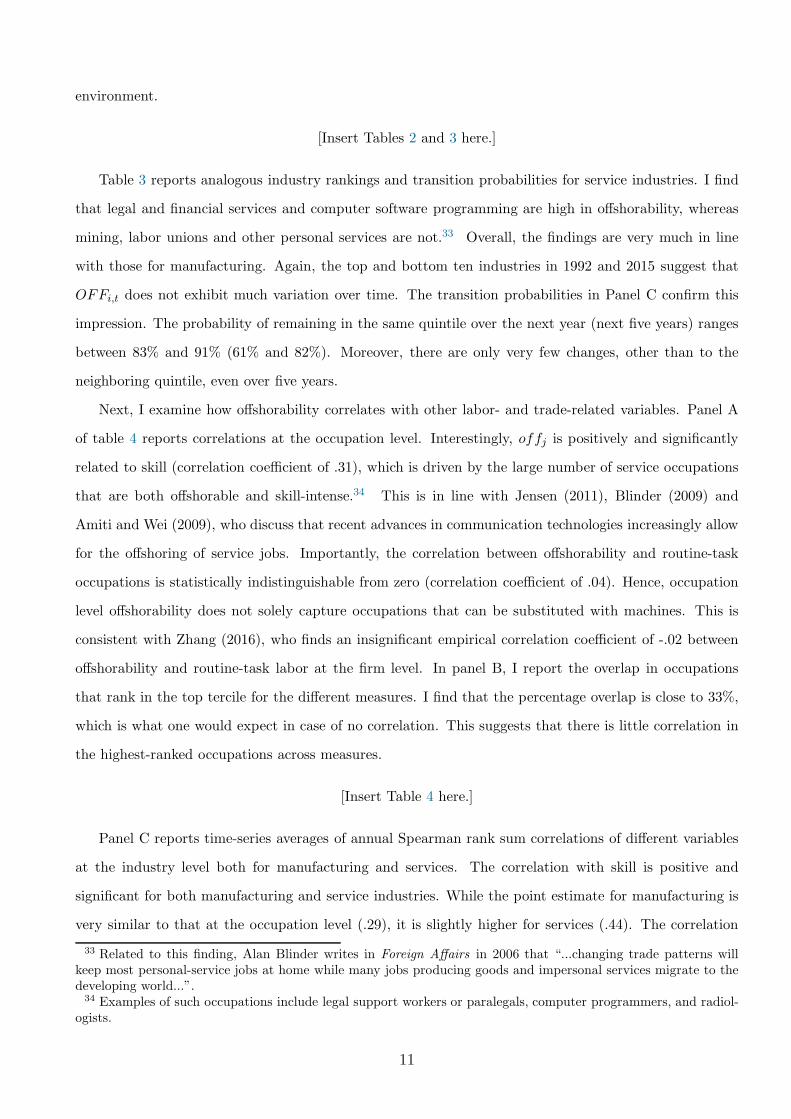
Table 3 reports analogous industry rankings and transition probabilities for service industries. I find

that legal and financial services and computer software programming are high in offshorability, whereas

mining, labor unions and other personal services are not.33 Overall, the findings are very much in line

with those for manufacturing. Again, the top and bottom ten industries in 1992 and 2015 suggest that

OFFi,t does not exhibit much variation over time. The transition probabilities in Panel C confirm this

impression. The probability of remaining in the same quintile over the next year (next five years) ranges

between 83% and 91% (61% and 82%). Moreover, there are only very few changes, other than to the

neighboring quintile, even over five years.

Next, I examine how offshorability correlates with other labor- and trade-related variables. Panel A

of table 4 reports correlations at the occupation level. Interestingly, offj is positively and significantly

related to skill (correlation coefficient of .31), which is driven by the large number of service occupations

that are both offshorable and skill-intense.34 This is in line with Jensen (2011), Blinder (2009) and

Amiti and Wei (2009), who discuss that recent advances in communication technologies increasingly allow

for the offshoring of service jobs. Importantly, the correlation between offshorability and routine-task

occupations is statistically indistinguishable from zero (correlation coefficient of .04). Hence, occupation

level offshorability does not solely capture occupations that can be substituted with machines. This is

consistent with Zhang (2016), who finds an insignificant empirical correlation coefficient of -.02 between

offshorability and routine-task labor at the firm level. In panel B, I report the overlap in occupations

that rank in the top tercile for the different measures. I find that the percentage overlap is close to 33%,

which is what one would expect in case of no correlation. This suggests that there is little correlation in

the highest-ranked occupations across measures.

[Insert Table 4 here.]

Panel C reports time-series averages of annual Spearman rank sum correlations of different variables

at the industry level both for manufacturing and services. The correlation with skill is positive and

significant for both manufacturing and service industries. While the point estimate for manufacturing is

very similar to that at the occupation level (.29), it is slightly higher for services (.44). The correlation

33 Related to this finding, Alan Blinder writes in Foreign Affairs in 2006 that “...changing trade patterns willkeep most personal-service jobs at home while many jobs producing goods and impersonal services migrate to thedeveloping world...”.34 Examples of such occupations include legal support workers or paralegals, computer programmers, and radiol-

ogists.

11

with routine is statistically indistinguishable from zero for both sectors (the point estimates are .10 for

manufacturing and .14 for services). Interestingly, the correlation with the labor mobility measure of

Donangelo (2014) is negative (-.22) and weakly statistically significant for manufacturing and is positive

(.11) but insignificant for services. The weak relationship with labor mobility is not surprising. Labor

mobility is intended to capture the transferability of occupation-specific skills across industries, which is

conceptually very different from offshorability.

Furthermore, I find that the correlation coefficient with product tradability from Jensen (2011) is pos-

itive (.13) but insignificant for manufacturing and positive and highly statistically significant for services

(.23).35 The insignificant correlation coefficient in manufacturing is not surprising. While offshorability

captures the “tradability” of the labor force, the measure by Jensen (2011) captures the tradability of the

product.

Finally, I also analyze the relation between OFFi,t and industry shipping costs, a variable often

employed in studies of international trade. I document a negative and weakly significant correlation co-

efficient (-0.16) between offshorability and shipping costs paid by importers for manufacturing industries.

For services, the lack of import data makes it impossible to calculate shipping costs at the industry level.

3.2 Portfolio Analysis

3.2.1 Offshorability Portfolios and Excess Returns

To study the characteristics of sample industries and realized excess returns, I construct five offshorability

portfolios. For each sample year, I assign industry offshorability in the previous year to individual stocks.

I then obtain monthly industry returns by value-weighting monthly stock returns. Again, industries are

defined at the 3-digit SIC level between 1990 and 2001 and at the 4-digit NAICS level between 2002 and

2016. In every year, at the end of June, I sort industry returns into five portfolios based on industry

offshorability quintiles. Finally, industry returns within each offshorability portfolio are either equal- or

value-weighted. To obtain value-weighted portfolio returns, I use an industry’s market capitalization as

a weight. In what follows, in the interest of brevity, I refer to industry excess returns simply as excess

returns. Panel A of table 5 reports the equal- and value-weighted excess returns of the five portfolios. L

(H) stands for the portfolio consisting of industries with low (high) offshorability, and L-H refers to the

strategy that is long L and short H.

[Insert Table 5 here.]

35 I thank J. Bradford Jensen for sharing his data on industry tradability. Jensen (2011) measures of industrytradability are based on geographic concentration/dispersion of production.

12

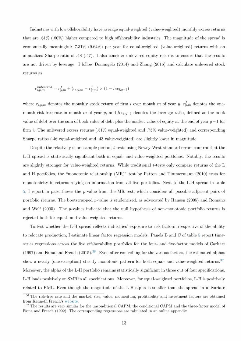
Industries with low offshorability have average equal-weighted (value-weighted) monthly excess returns

that are .61% (.80%) higher compared to high offshorability industries. The magnitude of the spread is

economically meaningful: 7.31% (9.64%) per year for equal-weighted (value-weighted) returns with an

annualized Sharpe ratio of .48 (.47). I also consider unlevered equity returns to ensure that the results

are not driven by leverage. I follow Donangelo (2014) and Zhang (2016) and calculate unlevered stock

returns as

runleveredi,y,m = rfy,m + (ri,y,m − rfy,m)× (1− levi,y−1)

where ri,y,m denotes the monthly stock return of firm i over month m of year y, rfy,m denotes the one-

month risk-free rate in month m of year y, and levi,y−1 denotes the leverage ratio, defined as the book

value of debt over the sum of book value of debt plus the market value of equity at the end of year y−1 for

firm i. The unlevered excess returns (.51% equal-weighted and .73% value-weighted) and corresponding

Sharpe ratios (.46 equal-weighted and .43 value-weighted) are slightly lower in magnitude.

Despite the relatively short sample period, t-tests using Newey-West standard errors confirm that the

L-H spread is statistically significant both in equal- and value-weighted portfolios. Notably, the results

are slightly stronger for value-weighted returns. While traditional t-tests only compare returns of the L

and H portfolios, the “monotonic relationship (MR)” test by Patton and Timmermann (2010) tests for

monotonicity in returns relying on information from all five portfolios. Next to the L-H spread in table

5, I report in parentheses the p-value from the MR test, which considers all possible adjacent pairs of

portfolio returns. The bootstrapped p-value is studentized, as advocated by Hansen (2005) and Romano

and Wolf (2005). The p-values indicate that the null hypothesis of non-monotonic portfolio returns is

rejected both for equal- and value-weighted returns.

To test whether the L-H spread reflects industries’ exposure to risk factors irrespective of the ability

to relocate production, I estimate linear factor regression models. Panels B and C of table 5 report time-

series regressions across the five offshorability portfolios for the four- and five-factor models of Carhart

(1997) and Fama and French (2015).36 Even after controlling for the various factors, the estimated alphas

show a nearly (one exception) strictly monotonic pattern for both equal- and value-weighted returns.37

Moreover, the alpha of the L-H portfolio remains statistically significant in three out of four specifications.

L-H loads positively on SMB in all specifications. Moreover, for equal-weighted portfolios, L-H is positively

related to HML. Even though the magnitude of the L-H alpha is smaller than the spread in univariate

36 The risk-free rate and the market, size, value, momentum, profitability and investment factors are obtainedfrom Kenneth French’s website.37 The results are very similar for the unconditional CAPM, the conditional CAPM and the three-factor model of

Fama and French (1992). The corresponding regressions are tabulated in an online appendix.

13

portfolio sorts, it is economically meaningful: the annualized alphas range between 3.82% and 6.49%,

with Sharpe ratios from .35 to .41.

3.2.2 Offshorability premium: Manufacturing vs Service Industries

Due to limited data availability, most empirical papers that study the effects of offshoring focus on U.S.

manufacturing firms or European data.38 Hence, having a measure of offshorability both for manufactur-

ing and services industries, it is interesting to see how the results differ among these two broad sectors.

To this end, I first split the sample into manufacturing and services and then conditionally sort industries

into five offshorability portfolios, as discussed above.39

Table 6 reports univariate portfolio sorts and CAPM regression results for manufacturing (Panel

A) and services (Panel B). The univariate sorts show that portfolio excess returns are decreasing in

offshorability in both sectors, which suggests that the relocation of production is a desirable option in

manufacturing and service industries. This is consistent with Jensen and Kletzer (2010), Blinder (2009)

and Amiti and Wei (2009), among others, who discuss the increasing importance of offshoring in service

industries.

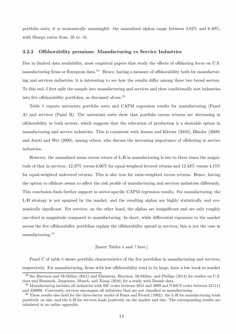
However, the annualized mean excess return of L-H in manufacturing is two to three times the magni-

tude of that in services: 12.37% versus 6.66% for equal-weighted levered returns and 12.43% versus 4.15%

for equal-weighted unlevered returns. This is also true for value-weighted excess returns. Hence, having

the option to offshore seems to affect the risk profile of manufacturing and services industries differently.

This conclusion finds further support in sector-specific CAPM regression results. For manufacturing, the

L-H strategy is not spanned by the market, and the resulting alphas are highly statistically and eco-

nomically significant. For services, on the other hand, the alphas are insignificant and are only roughly

one-third in magnitude compared to manufacturing. In short, while differential exposures to the market

across the five offshorability portfolios explain the offshorability spread in services, this is not the case in

manufacturing.40

[Insert Tables 6 and 7 here.]

Panel C of table 6 shows portfolio characteristics of the five portfolios in manufacturing and services,

respectively. For manufacturing, firms with low offshorability tend to be large, have a low book to market

38 See Harrison and McMillan (2011) and Ebenstein, Harrison, McMillan, and Phillips (2014) for studies on U.S.data and Hummels, Jørgensen, Munch, and Xiang (2016) for a study with Danish data.39 Manufacturing includes all industries with SIC codes between 2011 and 3999 and NAICS codes between 311111

and 339999. Conversely, services encompass all industries that are not classified as manufacturing.40 These results also hold for the three-factor model of Fama and French (1992): the L-H for manufacturing loads

positively on size, and the L-H for services loads positively on the market and size. The corresponding results aretabulated in an online appendix.

14

ratio, low market leverage and low labor intensity compared to high offshorability firms. For services, on

the other hand, the five portfolios show no clear patterns in terms of book to market ratio and market

leverage.

As a more restrictive test of the offshorability premium in manufacturing, I employ the four- and

five-factor models by Carhart (1997) and Fama and French (2015), respectively. The results are reported

in table 7. The alpha of the L-H strategy remains highly statistically and economically significant across

all specifications: the annualized alphas range between 8.05% and 9.94% with Sharpe ratios from .55 to

.81. Moreover, L-H positively loads on size and momentum.

To gain an idea of the performance of L-H in each sector over time, I plot the evolution of a one USD

investment on a log-scale in the left panel figure 1. The figure plots L-H separately for manufacturing

and service industries along the market, size and value. Both L-H portfolios significantly outperform the

size and value strategies over the period from July 1991 until June 2016.

[Insert Table 8 and Figure 1 here.]

Interestingly, the L-H strategy in manufacturing does not generally correlate strongly with the market

except during the financial crisis, when both investments lose value. The right panel of figure 1 plots the

realized equal-weighted excess returns of the L-H strategy in manufacturing along with average monthly

excess returns for the first and second half of the sample period. The two averages are similar in magnitude

(1.19% during 1991 and 2004 and 0.86% during 2004 and 2016), which suggests that the L-H strategy

delivers a stable return over time.

To further investigate the offshorability premium in manufacturing, I report portfolio sorts for different

time subsamples in table 8. The sample is split into four subsamples - one for each decade plus one that

excludes the financial crisis. The offshorability premium is, with one exception, positive and significant

in all subsamples. This is true both for equal- and value-weighted portfolios. For most subsamples, the

premium is significant at the 10% level due to the relatively small sample size and the corresponding loss

of statistical power. Moreover, the MR-test rejects the null hypothesis of non-monotonic portfolio returns

for all but the most recent subsample that runs from 2010:01 to 2016:06.41

In a next step, I investigate the predictive power of offshorability in the cross-section of returns. To

do so, I run annual panel regressions at the firm level. The regressions are of the following form:

ri,t = a+ bj,t + c ∗OFFi,t−1 + d ∗ controlsi,t−1 + ǫi,t, (3)

41 In a robustness test, I test whether the results are driven by the time variation in the OFFi,t measure. Ifind that keeping industry offshorability fixed over time (i.e., fixing it to the first observation for each industryclassification period) results in very similar full and subsample results. The corresponding results are tabulated inan online appendix.

15

where ri,t is the firm’s i annual stock return, a is a constant term, bj,t is an industry×year fixed effect,

OFFi,t−1 is lagged labor offshorability and controlsi,t−1 are lagged firm-level characteristics.42 I include

firm size, book-to-market ratio, market leverage ratio, hiring rate, investment rate, one-year lagged stock

return, operating leverage, and profitability to control for characteristics known to predict expected excess

returns. Standard errors are clustered at the firm and year level.

Table 9 reports the regression results for manufacturing in Panel A and services in Panel B. All vari-

ables are standardized with mean zero and variance one, which makes the coefficients directly comparable.

For manufacturing, the coefficient of offshorability is negative and statistically significant across all spec-

ifications. Moreover, the coefficients are only marginally affected by adding control variables individually

(compare regression specifications (1) to (9)), which is reassuring.43 The estimated slopes range from

-4.64 to -5.06 and are economically meaningful: a one standard deviation increase in offshorability is

associated with a 4% - 5% lower annual excess stock return.

[Insert Table 9 here.]

Regression specification (10) includes all control variables at once, which results in a reduction in sample

size. Nevertheless, the coefficient on OFFt−1 stays negative and highly statistically significant.44 For ser-

vices, the coefficients on offshorability are negative throughout all specifications. However, the coefficients

are statistically significant only in two regression specifications, which suggests that for services, OFFt−1

does not have much predictive power once controlled for other firm characteristics. This is consistent with

the findings of table 6.

3.3 Manufacturing Industries and the Surge in International Trade

Technological advances such as the revolution in information and communication technologies and the

dismantling of trade barriers have contributed to an increase in international trade activity over the recent

past. The left panel of figure 2 shows that the ratio of imports to U.S. Gross Domestic Product (GDP)

has increased by a factor of 1.5 over the sample period. Interestingly, this increase in imports/GDP is

mostly due to imports from low-wage countries, which have increased by a factor of 4.5 since 1990. By

contrast, high-wage country imports have increased by a factor of 1.2 only.45 These growth patterns are

42 Note that offshorability is measured at the industry level only. Hence, firms in a given industry and year sharethe same offshorability.43 I run similar monthly panel regressions following Belo, Lin, Li, and Zhao (2015) and find that the results are

nearly identical. The results are available upon request.44 These results are robust to various industry definitions. The corresponding results are tabulated in an online

appendix.45 I follow Bernard, Jensen, and Schott (2006a) and label a country as low-wage in year t if its GDP per capita is

less than 5% of the GDP per capita of the U.S. A list of countries that were classified as low-wage in every year ofthe sample period can be found in an online appendix.

16

illustrative of the change in the composition of U.S. imports, consistent with the principle of comparative

advantage first elaborated by Ricardo (1821) and continued by Heckscher (1919) and Ohlin (1933).46

They argue that countries have a comparative advantage in activities that are intensive in the use of

factors that are relatively abundant in the country. As a result, countries that have an abundance of

low-cost labor have an advantage in producing labor-intense products, and countries with an abundance

of skilled labor specialize in skill-intense products.

[Insert Figure 2 here.]

Another way of illustrating the change in the composition of U.S. imports is to look at the trade

balances for goods and services separately, as reported in the right panel of figure 2. While the trade

balance in goods has decreased sharply over the last 25 years, the trade balance in services has been positive

and slightly increasing since 1960. Hence, the United States is a net exporter in services.47 Consistent with

this, Jensen (2011) argues that providing services is consistent with the U.S.’s comparative advantage.

On the other hand, international specialization has led to fierce import competition in manufacturing

industries.48 In fact, many recent empirical studies stress the importance of international trade for

understanding the dynamics in U.S. manufacturing industries. In particular, the rise in import penetration

from low-wage countries has been emphasized as the key driving force of the decrease in manufacturing

employment (see, among others, Autor, Dorn, and Hanson (2013, 2016), Pierce and Schott (2016)).49

Motivated by this evidence, I examine how my results relate to import competition from low-wage

countries. I follow Bernard, Jensen, and Schott (2006a) and calculate import penetration from low-wage

countries at the industry level. Panel A of table 10 reports conditional double sorts on import penetration

and offshorability.50 Indeed, the L-H spread is monotonically increasing with import penetration both

for equal- and value-weighted returns. This finding is consistent with the interpretation that the ability

to relocate production is most valuable in industries that are exposed to fierce import competition from

low-wage countries.51

46 The figure that plots value shares of imports instead of real value of imports looks nearly identical. Thecorresponding figure can be found in the online appendix of the paper.47 In fact, the United States is the global leader in business service exports. The OECD reports that the United

States accounts for approximately 22 percent of the OECD total.48 The increase in imports is either due to new market entrants or imports of intermediate production inputs.

Antras (2015) reports that between 2000 and 2011, close to 50% of imports were intra-firm transactions, i.e., eitherintermediate production inputs or final goods manufactured entirely abroad. The other half of imports were eitherthird-party intermediate goods or final products of foreign competitors. Hence, the surge of imports from low-wagecountries over the past 25 years brought cheaper intermediate production inputs but also more fierce competitionto the U.S.49 While US total imports as a share of GDP have increased from 4.19% to 15.48% since 1960, US manufacturing

employment as a percent share of nonagricultural employment has fallen from 28.43% to 8.69%. A correspondingfigure can be found in the online appendix.50 I first sort on import penetration and then on offshorability.51 The results are very similar for double sorts on offshorability and import penetration from China, as reported

17

[Insert Tables 10 and 11 here.]

I also run cross-sectional return predictability regressions conditional on import penetration being

lower (higher) than the median, which allows me to control for various firm characteristics. The results

are reported in Panel B. Consistent with the double sorts, I find that coefficients on offshorability are

negative and significant only for firms in industries with high import penetration. Moreover, the absolute

values of the estimated coefficients on OFFt−1 are double the magnitude for high compared to low import

penetration industries.

A potential concern is that realized U.S. imports from low-wage countries may be correlated with

industry import demand shocks. To mitigate this concern, I instrument for import competition with

industries’ average shipping costs paid on imports, which serves as a proxy for barriers to trade. In the

data, industries with low shipping costs are associated with high imports and exports. Panel A of table 11

reports average returns of conditional double sorts on shipping costs and offshorability. The L-H spread is

monotonically decreasing with shipping costs, consistent with the findings in table 10. Panel B tabulates

the results of conditional panel regressions. Offshorability negatively predicts firms’ annual excess returns

only in industries with lower-than-median shipping costs.

Barrot, Loualiche, and Sauvagnat (2017) document that industries with low shipping costs face higher

import competition and have higher excess returns. This premium originates from the risk of displacement

of least efficient firms triggered by import competition. Given that the offshorability premium is increasing

in import penetration from low-wage countries and decreasing in shipping costs, my findings suggest that

offshoring helps protect industries from foreign competition. In particular, being able to offshore allows

firms to reduce their labor costs upon increases in competition. This argument is consistent with Magyari

(2017), who finds that offshoring enables US firms to reduce costs and outperform peers that cannot

offshore.

Table 4 shows that offshorability is slightly negatively related to shipping cost. Hence, one might

be concerned whether sorting on offshorability is similar to sorting on shipping costs. To mitigate this

concern, I replicate the findings of Barrot, Loualiche, and Sauvagnat (2017) for my sample period and

control for the return of the portfolio that is long firms in low shipping cost industries and short firms

in high shipping cost industries (henceforth, SC). The explanatory power of SC is very limited. In

fact, neither the monotonic relationship in the offshorability portfolio alphas nor the highly statistically

significant alpha of the L-H portfolio is impaired.52

in an online appendix.52 In a first step, I replicate the findings of Barrot, Loualiche, and Sauvagnat (2017). Despite different sample

periods, the resulting portfolio sorts look very similar to those in their paper. Portfolio sorts and the regressionresults are reported in the online appendix of this paper.

18

Approximately half of the manufacturing firms in my sample are multinational companies that have

sales in at least one country other than the United States. Fillat and Garetto (2015) have documented

that multinational firms experience higher stock returns compared to domestic firms. To understand how

their results relate to mine, I first split the sample into multinational and domestic manufacturing firms

and then conditionally sort them into five offshorability portfolios in each subsample. The results are

reported in panel A of table 12.

[Insert Table 12 here.]

In line with Fillat and Garetto (2015), I find that equal-weighted excess returns for multinationals

are higher than for domestic firms. Moreover, the L-H spread is positive, significant and of very similar

magnitude for both groups. This suggests that sorting on offshorability is different from sorting on a

firm’s location of sales. In addition, the non-monotonicity of portfolio excess returns can only be rejected

for firms with multinational operations. Panel B confirms that even after controlling for other firm

characteristics, offhsorability negatively predicts future annual excess returns both for multinational and

domestic firms.

Finally, given the large number of multinationals in manufacturing industries, another potential con-

cern is that L-H is related to differential foreign exchange exposures across industries. To address this,

I estimate three two-factor models including the U.S. market excess return and either the dollar factor,

the carry factor (both from Verdelhan (2017)) or the excess return of high interest rate currencies minus

low interest rate currencies (from Lustig, Roussanov, and Verdelhan (2011)). I find that the three factors

related to foreign exchange are insignificant in most specifications. Moreover, the L-H alphas are positive

and statistically different from zero in all specifications. The corresponding results are tabulated in an

online appendix.

4 Model

In this section, I develop a two-country dynamic general equilibrium trade model with multiple industries

that are heterogenous in their ability to offshore.

The model builds on existing work on trade models with aggregate risk by Ghironi and Melitz (2005)

and Barrot, Loualiche, and Sauvagnat (2017), who also focus on asset prices. To discuss my empirical

results through the lens of the model, I additionally embed firm-level offshoring, as in Antras and Helpman

(2004), in the model. Consequently, firms not only decide whether or not to export but also where to

produce their goods.

19

The model features two countries, West and East. To distinguish between the two countries, quantities

that refer to the East are labeled with a ⋆. Each country is inhabited by a continuum of homogenous

households and two industrial sectors that are spanned by S + 1 industries. The first sector consists of

one industry and a single homogenous good, and the corresponding sector quantities are labeled with a

0. The second sector encompasses S industries, which each consist of a continuum of differentiated goods

that are produced by a continuum of firms.

4.1 Demand Side: The Households Problem

Homogenous households have the following Epstein-Zin preferences over the consumption stream Ct:

Ut =

(1− β)C1−γν

t + β(

Et

[

U1−γt+1

]) 1ν

ν1−γ

where Ct is an aggregate consumption index, β is the subjective time discount factor, γ is the coefficient

of risk aversion, ψ is the elasticity of intertemporal substitution and ν ≡ 1−γ1−1/ψ is a parameter defined for

notational convenience. Each period, households derive utility from consuming goods in S+1 industries.

Ct is given by the following aggregator:

Ct = c1−a00,t

∑

s

δ1θs

(∫

Ωs,t

cs,t(ϕ)σs−1σs dϕ

) σsσs−1

θ−1θ

θθ−1

a0

,

where c0,t and 1−a0 denote, respectively, the consumption and the expenditure share in the homogenous

good sector; cs,t(ϕ) denotes the consumption of differentiated good variety ϕ in industry s; δs is an

industry taste parameter (where∑

s δs = 1); θ is the elasticity of substitution between industries; σs is

the elasticity of substitution among good varieties within industry s; and Ωs,t is the set of firms that sell

their goods at time t in industry s in the West.

The aggregation over industry-specific consumption and over varieties is based on constant elasticity

of substitution with elasticities θ and σs, respectively. This results in Dixit and Stiglitz (1977) demand

schedules at both the industry and the product level. Detailed derivations can be found in appendix A

of the paper.

Finally, households obtain revenues Lt from inelastic labor supply and from ownership of firms, re-

sulting in the following budget constraint:53

∑

s

∫

Ωs,t

ps,t(ϕ)cs,t(ϕ)dϕ ≤ Lt +Πt,

53 Wages in each country are equal to the numeraire and are set to 1 as discussed below.

20

with Πt being profits from firm ownership.54 In what follows, I suppress the time index t for ease of

notation.

4.2 Supply Side: Firms’ Production and Organizational Decision

Homogenous good sector - The homogenous good 0 is produced under constant returns to scale (CRS)

and a production function that is linear in labor.55 Moreover, the good is freely traded across countries.

Its price is used as a numeraire in each country and is set to one.56

Differentiated goods sector - This sector encompasses S industries that each consist of a continuum

of differentiated goods that are produced by a continuum of monopolistically competitive firms. Each

firm produces a different product variety, ϕ. Intuitively, firms possess a product variety-specific blueprint

that determines their idiosyncratic productivity. In what follows, ϕ not only serves as an identifier of

product variety but also stands for idiosyncratic productivity. Following Antras and Helpman (2004), I

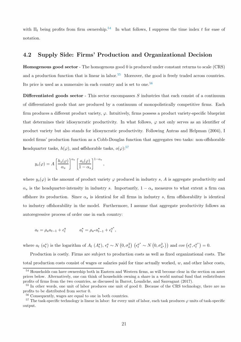
model firms’ production function as a Cobb-Douglas function that aggregates two tasks: non-offshorable

headquarter tasks, h(ϕ), and offshorable tasks, o(ϕ):57

ys(ϕ) = A

[hs(ϕ)

αs

]αs [ os(ϕ)

1− αs

]1−αs

,

where ys(ϕ) is the amount of product variety ϕ produced in industry s, A is aggregate productivity and

αs is the headquarter-intensity in industry s. Importantly, 1 − αs measures to what extent a firm can

offshore its production. Since αs is identical for all firms in industry s, firm offshorability is identical

to industry offshorability in the model. Furthermore, I assume that aggregate productivity follows an

autoregressive process of order one in each country:

at = ρaat−1 + ǫat a⋆t = ρa⋆a⋆t−1 + ǫa

⋆

t ,

where at (a⋆t ) is the logarithm of At (A

⋆t ), ǫ

at ∼ N

(0, σ2a

) (ǫa⋆

t ∼ N(0, σ2a⋆

))and cov

(ǫat , ǫ

a⋆t

)= 0.

Production is costly. Firms are subject to production costs as well as fixed organizational costs. The

total production costs consist of wages or salaries paid for time actually worked, w, and other labor costs,

54 Households can have ownership both in Eastern and Western firms, as will become clear in the section on assetprices below. Alternatively, one can think of households owning a share in a world mutual fund that redistributesprofits of firms from the two countries, as discussed in Barrot, Loualiche, and Sauvagnat (2017).55 In other words, one unit of labor produces one unit of good 0. Because of the CRS technology, there are no

profits to be distributed from sector 0.56 Consequently, wages are equal to one in both countries.57 The task-specific technology is linear in labor: for every unit of labor, each task produces ϕ units of task-specific

output.

21

c, such as payments to pension plans, unemployment insurance fees, legal costs and accruals for possible

severance payments. I assume that other labor costs are proportional to the amount of labor hired such

that the marginal costs of labor equals w + c. I further assume that any unit of labor can be employed

either as headquarter or offshorable tasks. In other words, within a country, there is no separation of the

labor force. For clarity of exposition, in what follows, I will be explicit about the total costs associated

with one unit of headquarter and offshorable labor employed in industry s. I call them wh,s and wo,s,

respectively.

Throughout the paper, I further assume that the East has a comparative cost advantage in offshorable

labor over the West. In particular, I assume that c > c⋆. That is, within the context of the model, the East

can be associated with a low-wage country such as China and the West with a highly developed economy

such as the U.S. Intuitively, the wedge c− c⋆ can be interpreted as differences in unemployment benefits

and other social insurances, strength of labor unions and severance payments across the two countries.

This cost wedge provides an incentive to Western firms to offshore and, as such, is a key ingredient for

the model to generate results consistent with the empirical evidence.

Given the comparative cost advantage of the East over the West, firms decide on their organizational

strategy along two dimensions. First, they decide whether to produce domestically or offshore part of

their production. Second, they choose whether to sell their output only domestically or, alternatively,

both on the domestic and export market. In what follows, I detail the optimal sorting of firms into the

different strategies.

Domestic Production vs Offshoring

Firms operate in monopolistically competitive industries and set their prices at a markup over marginal

costs. The monopolistic competition markup σsσs−1 is determined by the elasticity of substitution among

product varieties within an industry, σs.58 Hence, the price set by firms that produce domestically is

given by

ps,D(ϕ) =σs

σs − 1

(wh,s)αs(wo,s)

1−αs

Aϕ,

58 The higher the σs, the lower the markup σs

σs−1.

22

where wh,s (wo,s) are total wage costs for headquarter (offshorable) tasks. Firm profits in industry s are

defined as the difference between sales and total costs, Γs,D(ys,D(ϕ), ϕ):

πs,D(ϕ) = ps,D(ϕ)ys,D(ϕ) − Γs,D(ys,D(ϕ), ϕ)

=1

σsps,D(ϕ)

[ps,D(ϕ)

Ps

]−σs

Cs

= Bs((wh,s)

αs(wo,s)1−αs

)1−σs(Aϕ)σs−1 ,

where Bs = 1σs

[σsσs−1

]1−σsP σss Cs. Without loss of generality, fixed organizational costs for a purely

domestic firm are set to 0.59 Consequently, all firms in an industry are productive, since domestic

production is profitable for all values of ϕ.

Firms decide whether or not to offshore tasks of type o. On the one hand, firms that offshore can

benefit from potentially lower total production costs and from risk diversification.60 On the other hand,

offshoring is costly due to trade costs, τ⋆, and per-period fixed organizational costs of offshoring, fO.61

Trade costs are often associated with the costs of transporting intermediate inputs across countries.

Alternatively, τ⋆ can be interpreted more broadly to reflect other technological barriers related to inter-

national fragmentation, such as language barriers, communication or search costs.

As in Antras and Helpman (2004), fixed organizational costs, fO, can be interpreted as the joint man-

agement cost of final and intermediate goods production, such as supervision, quality control, accounting,

and marketing, which depend on the organizational form and location of production. These costs are

expressed in units of effective labor. I assume that firms hire workers from their respective domestic labor

markets to cover these fixed costs. Hence, profits with offshoring are equal to

πs,O(ϕ) = Bs((wh,s)

αs(w⋆o,sτ⋆)1−αs

)1−σs(

Aαs (A⋆)1−αs ϕ)σs−1

−fOA.

Profit-maximizing firms in industry s decide to offshore whenever profits from doing so are larger than

59 Alternatively, I could set the fixed costs for domestic production to a value different from zero. Consequently,firms with sufficiently low idiosyncratic productivity would decide to shut down production entirely. In the absenceof fixed costs for domestic production, fixed costs of offshoring, fO, can be interpreted as the excess cost of offshoringin comparison to domestic production.60 More formally, the total costs of producing y units of a final good of variety ϕ associated with Domestic sourcing

and Offshoring can be written as

Γs,D(ys,D(ϕ), ϕ) =ys,D(ϕ)

Aϕ(wh,s)

αs(wo,s)1−αs

Γs,O(ys,O(ϕ), ϕ) =fOA

+ys,O(ϕ)

Aαs (A⋆)1−αs ϕ

(wh,s)αs(w⋆

o,sτ⋆)1−αs

61 Notation: τ⋆ labels trade costs for shipments from East to West and τ labels trade costs for shipments fromWest to East.

23

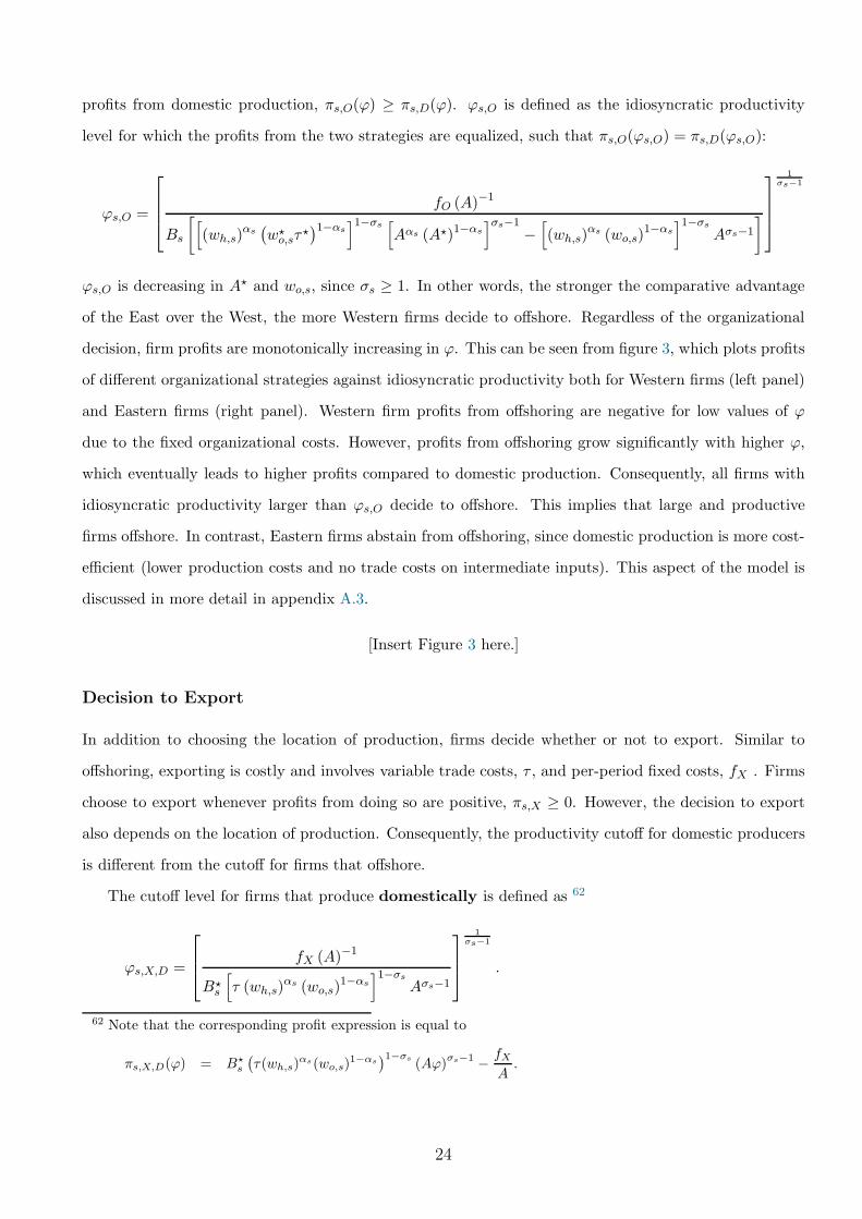
profits from domestic production, πs,O(ϕ) ≥ πs,D(ϕ). ϕs,O is defined as the idiosyncratic productivity

level for which the profits from the two strategies are equalized, such that πs,O(ϕs,O) = πs,D(ϕs,O):

ϕs,O =

fO (A)−1

Bs

[[

(wh,s)αs(w⋆o,sτ

⋆)1−αs

]1−σs [

Aαs (A⋆)1−αs]σs−1

−[

(wh,s)αs (wo,s)

1−αs]1−σs

Aσs−1

]

1σs−1

ϕs,O is decreasing in A⋆ and wo,s, since σs ≥ 1. In other words, the stronger the comparative advantage

of the East over the West, the more Western firms decide to offshore. Regardless of the organizational

decision, firm profits are monotonically increasing in ϕ. This can be seen from figure 3, which plots profits

of different organizational strategies against idiosyncratic productivity both for Western firms (left panel)

and Eastern firms (right panel). Western firm profits from offshoring are negative for low values of ϕ

due to the fixed organizational costs. However, profits from offshoring grow significantly with higher ϕ,

which eventually leads to higher profits compared to domestic production. Consequently, all firms with

idiosyncratic productivity larger than ϕs,O decide to offshore. This implies that large and productive

firms offshore. In contrast, Eastern firms abstain from offshoring, since domestic production is more cost-

efficient (lower production costs and no trade costs on intermediate inputs). This aspect of the model is

discussed in more detail in appendix A.3.

[Insert Figure 3 here.]

Decision to Export

In addition to choosing the location of production, firms decide whether or not to export. Similar to

offshoring, exporting is costly and involves variable trade costs, τ , and per-period fixed costs, fX . Firms

choose to export whenever profits from doing so are positive, πs,X ≥ 0. However, the decision to export

also depends on the location of production. Consequently, the productivity cutoff for domestic producers

is different from the cutoff for firms that offshore.

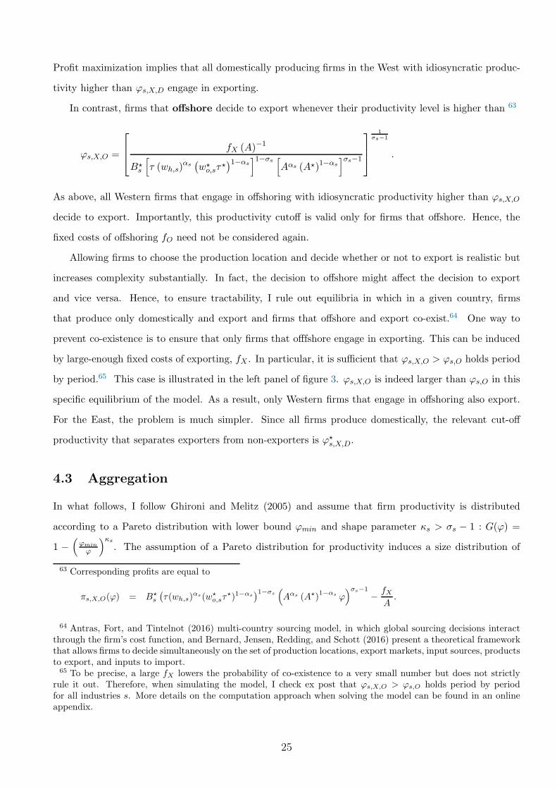
The cutoff level for firms that produce domestically is defined as 62

ϕs,X,D =

fX (A)−1

B⋆s

[

τ (wh,s)αs (wo,s)

1−αs]1−σs

Aσs−1

1σs−1

.

62 Note that the corresponding profit expression is equal to

πs,X,D(ϕ) = B⋆s

(τ(wh,s)

αs(wo,s)1−αs

)1−σs(Aϕ)

σs−1−fXA.

24

Profit maximization implies that all domestically producing firms in the West with idiosyncratic produc-

tivity higher than ϕs,X,D engage in exporting.

In contrast, firms that offshore decide to export whenever their productivity level is higher than 63

ϕs,X,O =

fX (A)−1

B⋆s

[

τ (wh,s)αs(w⋆o,sτ

⋆)1−αs

]1−σs [

Aαs (A⋆)1−αs]σs−1

1σs−1

.

As above, all Western firms that engage in offshoring with idiosyncratic productivity higher than ϕs,X,O

decide to export. Importantly, this productivity cutoff is valid only for firms that offshore. Hence, the

fixed costs of offshoring fO need not be considered again.

Allowing firms to choose the production location and decide whether or not to export is realistic but

increases complexity substantially. In fact, the decision to offshore might affect the decision to export

and vice versa. Hence, to ensure tractability, I rule out equilibria in which in a given country, firms

that produce only domestically and export and firms that offshore and export co-exist.64 One way to

prevent co-existence is to ensure that only firms that offfshore engage in exporting. This can be induced

by large-enough fixed costs of exporting, fX . In particular, it is sufficient that ϕs,X,O > ϕs,O holds period

by period.65 This case is illustrated in the left panel of figure 3. ϕs,X,O is indeed larger than ϕs,O in this

specific equilibrium of the model. As a result, only Western firms that engage in offshoring also export.

For the East, the problem is much simpler. Since all firms produce domestically, the relevant cut-off

productivity that separates exporters from non-exporters is ϕ⋆s,X,D.

4.3 Aggregation

In what follows, I follow Ghironi and Melitz (2005) and assume that firm productivity is distributed

according to a Pareto distribution with lower bound ϕmin and shape parameter κs > σs − 1 : G(ϕ) =

1 −(ϕminϕ

)κs. The assumption of a Pareto distribution for productivity induces a size distribution of

63 Corresponding profits are equal to

πs,X,O(ϕ) = B⋆s

(τ(wh,s)

αs(w⋆o,sτ

⋆)1−αs)1−σs

(

Aαs (A⋆)1−αs ϕ

)σs−1

−fXA.

64 Antras, Fort, and Tintelnot (2016) multi-country sourcing model, in which global sourcing decisions interactthrough the firm’s cost function, and Bernard, Jensen, Redding, and Schott (2016) present a theoretical frameworkthat allows firms to decide simultaneously on the set of production locations, export markets, input sources, productsto export, and inputs to import.65 To be precise, a large fX lowers the probability of co-existence to a very small number but does not strictly

rule it out. Therefore, when simulating the model, I check ex post that ϕs,X,O > ϕs,O holds period by periodfor all industries s. More details on the computation approach when solving the model can be found in an onlineappendix.

25

firms that is also Pareto, which fits well the empirical distribution. The parameter κs relates industry

output to the cross-section of firms, where high values are associated with more homogenous industries

in the sense that more output is concentrated among the smallest and least-productive firms.

Quantities

As in Melitz (2003) and Ghironi and Melitz (2005), it is enough to track the mass and the average

productivity for firms that choose the same strategy. In essence, the model is isomorphic to one in which

firms within a strategy group all have a productivity equal to the average productivity of the group.

Put differently, the average productivity levels per group summarize all information on the productivity

distribution relevant for macroeconomic variables.

First, I calculate the fraction of firms in industry s that engage in domestic production, ζs,D, and

offshoring, ζs,O. Moreover, ζs,X,O and ζ⋆s,X,D stand for the fractions of firms that export in the West and

East, respectively. These quantities are determined by the cutoff productivity levels and the shape of the

Pareto distribution, as detailed in appendices A.2 and A.3.

Second, I derive average productivity levels for the different groups: 1) ϕs,D, for purely domestic West-

ern firms; 2) ϕs,O, for Western firms that offshore; 3) ϕs,X,O, for Western firms that offshore and export;

4) ϕ⋆s,D, for purely domestic Estern firms; and 5) ϕ⋆s,X,D, for Eastern firms that produce domestically and

export. These quantities can be calculated as simple conditional averages for the Pareto distribution.

Again, detailed derivations can be found in appendices A.2 and A.3.

Industry Profits and Prices

Industry-wide profits and price indices can now be calculated using probability masses and average pro-

ductivity levels. Industry profits are simply given by the sum of the profits made on the domestic and

exporting markets. Therefore, industry profits in the West are given by

Πs = Ns [ζs,Dπs,D(ϕs,D) + ζs,Oπs,O(ϕs,O) + ζs,X,Oπs,X,O(ϕs,X,O)]

and industry profits in the East are given by

Π⋆s = N⋆s

[π⋆s,D(ϕ

⋆s,D) + ζ⋆s,X,Dπ

⋆s,X,D(ϕ

⋆s,X,D)

],

where Ns (N⋆s ) is the total mass of firms in the West (East) exogenously set to match the size of the

economy.

26

Finally, the industry price indices in the two countries are equal to

Ps =[

Ns

[ζs,Dps,D(ϕs,D)

1−σs + ζs,Ops,O(ϕs,O)1−σs

]+N⋆

s ζ⋆s,X,D

(p⋆s,X,D(ϕ

⋆s,X,D)

)1−σs] 1

1−σs ,

in the West, and

P ⋆s =[N⋆s p

⋆s,D(ϕ

⋆s,D)

1−σs +Nsζs,X,Ops,X,O(ϕs,X,O)1−σs

] 11−σs ,

in the East.

4.4 Equilibrium

In equilibrium, the aggregate budget constraint of the representative household is given in terms of the

aggregate price index P , composite consumption C, labor income L and revenues from Western and

Eastern industries, Πs and Π⋆s:

PC ≤ L+∑

s

Πs + χ

[Ns

Ns +N⋆s

Π⋆s −N⋆s

Ns +N⋆s

Πs

]

.

The exogenous parameter χ ∈ [0, 1] controls the level of risk sharing across countries in the economy.

This formulation embeds both the case of no risk-sharing and perfect or full risk-sharing. Without risk-

sharing, χ = 0, households only receive dividends from domestic firms: Πno =∑

sΠs. In comparison,

with full risk-sharing, χ = 1, households receive a share of total world profits that is proportional to

their capital endowments: Πfull =∑

sNs

Ns+N⋆s(Πs +Π⋆s). Consequently, dividends paid to households are

a convex combination of Πno and Πfull.

The model is solved with time-invariant mass of firms in each industry. Moreover, the model abstracts

from capital or investment. As a result, firms can adjust their production solely by deciding either to

offshore or export. The equilibrium is defined as a collection of prices (ps,D, ps,O, ps,X,O, ps,X,D, Ps, PT , P ),

output (ys (ϕ)), consumption (cs (ϕ)) and labor demand (ls (ϕ)) such that each firm maximizes profit,

consumers maximize their utility, and goods and labor markets clear.

4.5 Asset Pricing

Since the representative household in the West holds Western firms, the firms are priced using her stochas-

tic discount factor (SDF). Therefore, I derive the Euler equation from the portfolio problem faced by the

representative household. She maximizes her continuation utility over the consumption stream Ct sub-

ject to her budget constraint. Because there is no capital and investment in the model, firms pay out

27

dividends that are equal to their profits, πs,t(ϕ).

max

(1− β)C1−γν

t + β(

Et

[

U1−γt+1

]) 1ν

ν1−γ

s.t. PtCt +∑

s

∫

Ωs

xs,t+1(ϕ)υs,t(ϕ)dϕ ≤ L+∑

s

∫

Ωs

xs,t(ϕ) [υs,t(ϕ) + πs,t(ϕ)] dϕ

where xs,t(ϕ) is the investment in the firm in industry s of variety ϕ and υs,t(ϕ) is the corresponding firm

valuation.

The resulting Euler equation reads as follows:

υs,t = Et [Mt,t+1 (υs,t+1(ϕ) + πs,t+1(ϕ))] ,

where Mt,t+1 = βν∆C−νψ

t Rν−1c,t is the stochastic discount factor (SDF) and Rc,t is the return on the

consumption claim.

4.6 Calibration

To calibrate my model, I associate the West with the United States and the East with China. Moreover,

where possible, I calibrate the model using parameters from the literature, as reported in table 13. In

particular, I use elasticities across industries from Loualiche (2015) and across goods from Broda and

Weinstein (2006). The firm distribution is governed by the parameter κs, which is set to 3.4, as in

Ghironi and Melitz (2005). The industry taste parameter δs is equal to 0.5. Hence, households do not

have a preference for a certain industry.

[Insert Table 13 here.]

Wage costs other than pay for time in the West, c, are chosen to match the empirical counterpart in

the United States. According to the Bureau of Labor Statistics (BLS), 24.35% of the total wage costs in

manufacturing accounted for social insurance payments and 8.92% for directly paid benefits.66 Hence,

33.27% of the total wage bill consisted of payments other than wages and salaries for time actually worked.

To reflect this in the model, I calibrate c to 0.32 and c⋆ to 0, assuming absence of social insurance costs

in the East.

L and L⋆ are determined by the ratio of the working age population in the U.S. and China. The

Federal Reserve Bank of St. Louis reports a working age population of 205 millions by the end of 2015 in

the U.S. and 1’004 million in China. The mass of firms in each country, Ns and N⋆s , is chosen to match

66 Directly paid benefits are primarily pay for leave time, bonuses, and pay in kind.

28

the ratio of the market capitalization in the U.S. and China. The World Bank states the total market

capitalization of listed domestic companies in 2015 as 25.068 trillion USD in the U.S. and 8.19 trillion

USD in China. To match the ratio between the two, I calculate the model-implied ratio of the sum of

market values of all firms in the West and East, respectively.

The headquarter intensities of the two industries, αs, are set to 0.55 and 0.95, respectively. This

implies that a high (low) offshorability industry has an offshoring potential of 45% (5%) and that the

average offshoring potential in the model economy is 25%. For comparison, the OECD estimates that

close to 20% of jobs in OECD countries are offshorable, while Blinder’s (2009) estimates for the U.S. lie

between 22% and 29%.67

Variable trade cost and fixed cost parameters are set to the values in Ghironi and Melitz (2005) and

Barrot, Loualiche, and Sauvagnat (2017), respectively. The subjective discount factor is 0.99, and the

intertemporal elasticity of substitution is 1.5, as in Bansal and Yaron (2004). I calibrate the risk aversion

parameter to match the U.S. equity premium. Finally, parameters related to aggregate productivity in the

West (East) are chosen to reflect GDP in the U.S. (Chinese imports to the U.S.), as in Barrot, Loualiche,

and Sauvagnat (2017).

4.7 Model Mechanism

Consumption Response - To examine what drives asset prices in the model, it is necessary to under-

stand how aggregate consumption and the SDF respond to aggregate productivity shocks in the model.

The elasticity of consumption in the West to a productivity shock in the East, η⋆ (C)68 , is

η⋆ (C) = −η⋆ (P )︸ ︷︷ ︸

price effect

+Π

L+Πη⋆ (Π)

︸ ︷︷ ︸

wealth effect

(4)

The elasticity consists of a price and a wealth effect. As will be discussed later, the elasticity of the price

index with respect to A⋆ is negative. As a result, the sign of the first term is unambiguously positive. On

the other hand, the sign of the wealth effect depends on the degree of international risk sharing. With

full risk-sharing, the wealth effect is positive, as is the elasticity of consumption with respect to a foreign

productivity shock: Western households benefit from (1) lower domestic prices due to increases in imports

and (2) higher capital income due to higher world profits.

However, with a sufficiently high degree of home bias in capital income (low χ), the wealth effect is

67 The OECD also reports the offshoring potential for NACE 2-digit industries. For the year 2003, the numberslie between 79.5% and 1.8%.68 Notation: η (X) = ∂ logX

∂ logAand η⋆ (X) = ∂ logX

∂ logA⋆ .

29

negative and dominates the positive price effect. As an illustration, the first row of figure 4 plots impulse

response functions of consumption for different values of χ. In the baseline parametrization, χ < 0.75

is sufficient to generate a negative consumption response. χ = 0.75 implies that Western households

overweigh their investments in domestic firms by 18.62% compared to domestic firms’ share of the world

market. Hence, a fairly moderate home bias is sufficient to generate a negative elasticity of consumption

with respect to a positive productivity shock in the East. In comparison, Coeurdacier and Rey (2012)

empirically find a home bias for equity investments of 44.6% in the U.S. in 2008.69 To simplify the

exposition, I impose no international risk sharing (i.e., χ = 0) in my benchmark specification; I then

discuss the implications thereof.

[Insert Figures 4 and 5 here.]

The elasticity of consumption to productivity shocks in the West looks identical to equation 4. For

shocks to A, however, the elasticity of consumption is unambiguously positive. In particular, both price

and wealth effect carry a positive sign.

In what follows, I separately discuss how shocks to A⋆ and A affect the equilibrium. The discussion

mostly focuses on the West as the main country of interest and starts with the analysis of aggregate

productivity shocks in the East.

Shocks to A⋆ - To facilitate the discussion, figure 4 plots impulse response functions of model quantities

to a positive one standard deviation shock to A⋆ in the absence of risk sharing. As discussed, consumption

in the West (East) decreases (increases) upon arrival of a shock. Moreover, due to higher productivity,

more Eastern firms find it profitable to export, which results in an increase in import penetration. Higher

import penetration in turn leads to an increase in product variety, a decrease in industry prices and a

loss in market share and profits of Western firms.

Higher productivity in the East, however, also renders offshoring more attractive. Doing so allows firms

to lower costs, which goes hand in hand with a larger market share and higher profits. Hence, offshoring

effectively acts as partial insurance against adverse consequences associated with foreign productivity

shocks.

The response of the fraction of firms that offshore is more pronounced in high offshorability industries.

The reason is simple: in the model, industries with higher offshoring potential are able to replace more

workers/tasks, which results in a larger cost reduction and makes it more likely for firms to overcome the

fixed costs of offshoring. As a result, profits drop less in industries with high offshorability.

69 For further empirical evidence of home bias in the U.S., see, among others, French and Poterba (1991) andCoval and Moskowitz (1999); and for rational explanations of the home bias puzzle, see, for example, Glassmanand Riddick (2001), Ahearne, Griever, and Warnock (2004), Nieuwerburgh and Veldkamp (2009) and Bretscher,Julliard, and Rosa (2016).

30

What does this mean for asset prices? The heterogenous response of industry profits maps into

differential asset price and excess return dynamics across industries. The last row plots the response of

the SDF, asset prices and excess returns for the case of no and full risk sharing, respectively. Consistent

with the consumption response in the first row, the SDF increases under no risk sharing but decreases

with full risk sharing. However, the qualitative response of asset prices and returns is not altered by

the degree of risk sharing. In both cases, the responses are negative and more pronounced for the low

offshorability industry.

Shocks to A - Figure 5 plots the impulse responses to a negative one standard deviation shock to A.

I plot the responses to a negative productivity shock to facilitate comparison with the impulse response

functions after a shock to A⋆. Upon arrival of the shock, Western consumption drops, which affects firms

through a decrease in product demand. Moreover, because the production function of Eastern firms that

export to the West is not directly affected by shocks to A, their productivity and, hence, their prices

remain unchanged. This gives Eastern exporters a competitive advantage over Western firms whenever a

negative shock to A happens. As a result, Western firms lose market share to these exporters.

As above, offshoring presents itself as a valuable alternative in order to mitigate the adverse con-

sequences of the shock. Again, offshoring results in a larger cost reduction for high compared to low

offshorability industries. Consequently, the response of the fraction of firms that offshore is more pro-

nounced in high offshorability industries, which ultimately leads to smoother industry profits. Asset prices

and excess returns follow from industry profits and look very similar to figure 4 (not shown).

To sum up, the ability to offshore protects industries against losses associated with import competition.

Differences in offshorability across industries contribute to a spread in excess returns similar to the L-H

spread observed in the data.

4.8 Model Simulation Results

To quantify the model and investigate the contribution of the two productivity shocks, I calculate moments

from simulated data. As discussed in section 4.6, I target the ratios of market capitalization and working

age populations in the U.S. and China as well as the average import competition from China to discipline

my calibration exercise. In particular, matching these moments constrains the choice of parameters Ns,

N⋆s , L, L

⋆ and f⋆X . The model matches the targeted moments well, as can be seen in panel A of table 14.

[Insert Table 14 here.]

Panel B of the same table reports model-implied macro moments. Similar to Barrot, Loualiche, and

Sauvagnat (2017), aggregate consumption is too volatile in the model. While the mean of the risk-free

31

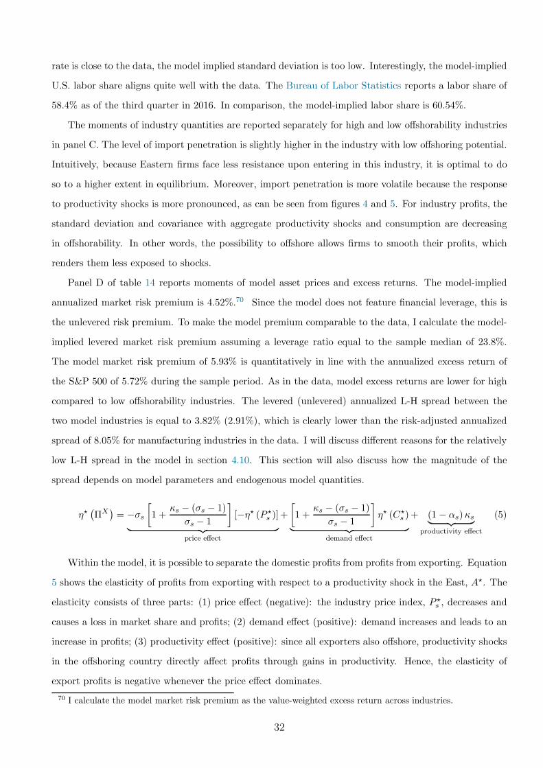
rate is close to the data, the model implied standard deviation is too low. Interestingly, the model-implied

U.S. labor share aligns quite well with the data. The Bureau of Labor Statistics reports a labor share of

58.4% as of the third quarter in 2016. In comparison, the model-implied labor share is 60.54%.

The moments of industry quantities are reported separately for high and low offshorability industries

in panel C. The level of import penetration is slightly higher in the industry with low offshoring potential.

Intuitively, because Eastern firms face less resistance upon entering in this industry, it is optimal to do

so to a higher extent in equilibrium. Moreover, import penetration is more volatile because the response

to productivity shocks is more pronounced, as can be seen from figures 4 and 5. For industry profits, the

standard deviation and covariance with aggregate productivity shocks and consumption are decreasing

in offshorability. In other words, the possibility to offshore allows firms to smooth their profits, which

renders them less exposed to shocks.

Panel D of table 14 reports moments of model asset prices and excess returns. The model-implied

annualized market risk premium is 4.52%.70 Since the model does not feature financial leverage, this is

the unlevered risk premium. To make the model premium comparable to the data, I calculate the model-

implied levered market risk premium assuming a leverage ratio equal to the sample median of 23.8%.

The model market risk premium of 5.93% is quantitatively in line with the annualized excess return of

the S&P 500 of 5.72% during the sample period. As in the data, model excess returns are lower for high

compared to low offshorability industries. The levered (unlevered) annualized L-H spread between the

two model industries is equal to 3.82% (2.91%), which is clearly lower than the risk-adjusted annualized

spread of 8.05% for manufacturing industries in the data. I will discuss different reasons for the relatively

low L-H spread in the model in section 4.10. This section will also discuss how the magnitude of the

spread depends on model parameters and endogenous model quantities.

η⋆(ΠX)= −σs

[

1 +κs − (σs − 1)

σs − 1

]

[−η⋆ (P ⋆s )]

︸ ︷︷ ︸

price effect

+

[

1 +κs − (σs − 1)

σs − 1

]

η⋆ (C⋆s )

︸ ︷︷ ︸

demand effect

+ (1− αs)κs︸ ︷︷ ︸

productivity effect

(5)

Within the model, it is possible to separate the domestic profits from profits from exporting. Equation

5 shows the elasticity of profits from exporting with respect to a productivity shock in the East, A⋆. The

elasticity consists of three parts: (1) price effect (negative): the industry price index, P ⋆s , decreases and

causes a loss in market share and profits; (2) demand effect (positive): demand increases and leads to an

increase in profits; (3) productivity effect (positive): since all exporters also offshore, productivity shocks

in the offshoring country directly affect profits through gains in productivity. Hence, the elasticity of

export profits is negative whenever the price effect dominates.

70 I calculate the model market risk premium as the value-weighted excess return across industries.

32

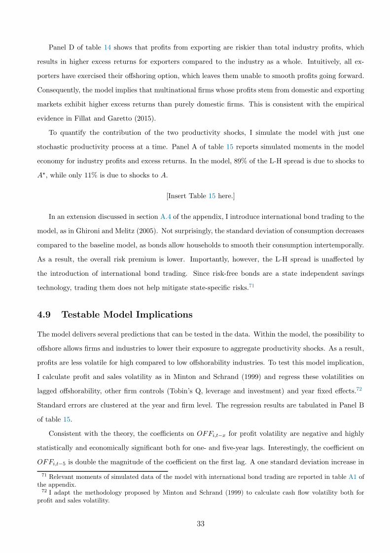
Panel D of table 14 shows that profits from exporting are riskier than total industry profits, which

results in higher excess returns for exporters compared to the industry as a whole. Intuitively, all ex-

porters have exercised their offshoring option, which leaves them unable to smooth profits going forward.

Consequently, the model implies that multinational firms whose profits stem from domestic and exporting

markets exhibit higher excess returns than purely domestic firms. This is consistent with the empirical

evidence in Fillat and Garetto (2015).

To quantify the contribution of the two productivity shocks, I simulate the model with just one

stochastic productivity process at a time. Panel A of table 15 reports simulated moments in the model

economy for industry profits and excess returns. In the model, 89% of the L-H spread is due to shocks to

A⋆, while only 11% is due to shocks to A.

[Insert Table 15 here.]

In an extension discussed in section A.4 of the appendix, I introduce international bond trading to the

model, as in Ghironi and Melitz (2005). Not surprisingly, the standard deviation of consumption decreases

compared to the baseline model, as bonds allow households to smooth their consumption intertemporally.

As a result, the overall risk premium is lower. Importantly, however, the L-H spread is unaffected by

the introduction of international bond trading. Since risk-free bonds are a state independent savings

technology, trading them does not help mitigate state-specific risks.71

4.9 Testable Model Implications

The model delivers several predictions that can be tested in the data. Within the model, the possibility to

offshore allows firms and industries to lower their exposure to aggregate productivity shocks. As a result,

profits are less volatile for high compared to low offshorability industries. To test this model implication,

I calculate profit and sales volatility as in Minton and Schrand (1999) and regress these volatilities on

lagged offshorability, other firm controls (Tobin’s Q, leverage and investment) and year fixed effects.72

Standard errors are clustered at the year and firm level. The regression results are tabulated in Panel B

of table 15.

Consistent with the theory, the coefficients on OFFi,t−x for profit volatility are negative and highly

statistically and economically significant both for one- and five-year lags. Interestingly, the coefficient on

OFFi,t−5 is double the magnitude of the coefficient on the first lag. A one standard deviation increase in

71 Relevant moments of simulated data of the model with international bond trading are reported in table A1 ofthe appendix.72 I adapt the methodology proposed by Minton and Schrand (1999) to calculate cash flow volatility both for

profit and sales volatility.

33

industry offshorability is associated with an 8.9% (one-year lag) to 19.7% (five-year lag) decrease in the

profit volatility for the median firm. Regression coefficients for several lags with 90% and 95% confidence

bands are plotted in figure 6. I find that the coefficient on OFFi,t−x is monotonically increasing in

magnitude with the horizon. This is consistent with offshoring being a process that takes time to be fully

incorporated.

[Insert Figure 6 here.]

The results for sales volatility are very similar as for profit volatility. While the coefficients on OFFi,t−x

are negative in all specifications, they are statistically different from zero at a 90% (95%) confidence level

only for horizons larger or equal to three (four) years. Intuitively, offshoring allows for a cost reduction

that affects profits with higher immediacy than sales.

Furthermore, the model allows one to form predictions about the cross-sectional dispersion of the L-H

premium. Households become more price-sensitive when the elasticity of substitution among product

varieties, σs, increases. Put differently, in industries with high elasticities, all else being equal, the drop

in Western firms’ market share is more pronounced upon arrival of an adverse productivity shock - both

in low and high offshorability industries. This can be seen from the elasticity of domestic profits with

respect to a productivity shock in the East:

η⋆(ΠD)

= − (σs − θ) (−η⋆ (Ps))︸ ︷︷ ︸

competition effect

+ η⋆ (Cs) +1− a0 − θ

a0(−η⋆ (P ))

︸ ︷︷ ︸

expenditure effect

+

κsζs,O (πs,O − πs,D)

ΠD︸ ︷︷ ︸

relative benefits from offshoring

− (σs − 1)ζs,Dπs,DΦ+ ζs,Oπs,O

ΠD︸ ︷︷ ︸

industry composition effect

(−η⋆ (ϕs,O)) +

ζs,Oπs,OΠD

(σs − 1) (1− αs)︸ ︷︷ ︸

productivity gain from offshoring

, (6)

where Φ > 0 and ∂Φ∂ϕs,O

> 0.73 Irrespective of an industry’s offshorability, the elasticity is more negative

with higher σs because the competition effect is amplified. Competition leads to a decrease in industry

prices, which results in a decrease in market share. Moreover, the effect of an increase in σs depends

on the industry equilibrium in the West (industry composition effect). A higher elasticity of substitution

73 ϕ is defined as follows:

Φ =ϕκs

s,min

σs − 1

ϕσs−κs

s,O [κs − (σs − 1)]

ϕσs−1s,min − ϕκs

s,min1

ϕκs−(σs−1)s,O

−κs

ϕκs

s,O − ϕκs

s,min

34

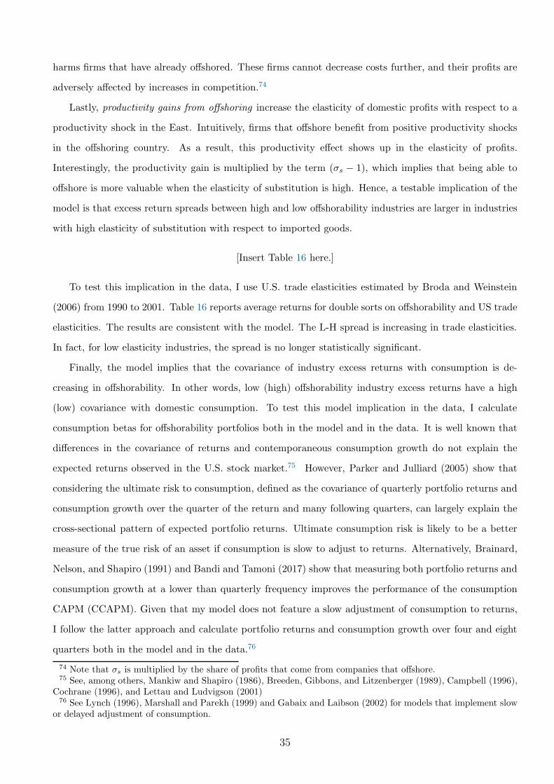
harms firms that have already offshored. These firms cannot decrease costs further, and their profits are

adversely affected by increases in competition.74

Lastly, productivity gains from offshoring increase the elasticity of domestic profits with respect to a

productivity shock in the East. Intuitively, firms that offshore benefit from positive productivity shocks

in the offshoring country. As a result, this productivity effect shows up in the elasticity of profits.

Interestingly, the productivity gain is multiplied by the term (σs − 1), which implies that being able to

offshore is more valuable when the elasticity of substitution is high. Hence, a testable implication of the

model is that excess return spreads between high and low offshorability industries are larger in industries

with high elasticity of substitution with respect to imported goods.

[Insert Table 16 here.]

To test this implication in the data, I use U.S. trade elasticities estimated by Broda and Weinstein

(2006) from 1990 to 2001. Table 16 reports average returns for double sorts on offshorability and US trade

elasticities. The results are consistent with the model. The L-H spread is increasing in trade elasticities.

In fact, for low elasticity industries, the spread is no longer statistically significant.

Finally, the model implies that the covariance of industry excess returns with consumption is de-

creasing in offshorability. In other words, low (high) offshorability industry excess returns have a high

(low) covariance with domestic consumption. To test this model implication in the data, I calculate

consumption betas for offshorability portfolios both in the model and in the data. It is well known that

differences in the covariance of returns and contemporaneous consumption growth do not explain the

expected returns observed in the U.S. stock market.75 However, Parker and Julliard (2005) show that

considering the ultimate risk to consumption, defined as the covariance of quarterly portfolio returns and

consumption growth over the quarter of the return and many following quarters, can largely explain the

cross-sectional pattern of expected portfolio returns. Ultimate consumption risk is likely to be a better

measure of the true risk of an asset if consumption is slow to adjust to returns. Alternatively, Brainard,

Nelson, and Shapiro (1991) and Bandi and Tamoni (2017) show that measuring both portfolio returns and

consumption growth at a lower than quarterly frequency improves the performance of the consumption

CAPM (CCAPM). Given that my model does not feature a slow adjustment of consumption to returns,

I follow the latter approach and calculate portfolio returns and consumption growth over four and eight

quarters both in the model and in the data.76

74 Note that σs is multiplied by the share of profits that come from companies that offshore.75 See, among others, Mankiw and Shapiro (1986), Breeden, Gibbons, and Litzenberger (1989), Campbell (1996),

Cochrane (1996), and Lettau and Ludvigson (2001)76 See Lynch (1996), Marshall and Parekh (1999) and Gabaix and Laibson (2002) for models that implement slow

or delayed adjustment of consumption.

35

[Insert Table 17 here.]

Panel A of table 17 reports the regression results for the simulated data. As discussed above, the

consumption beta is higher for low compared to high offshorability industries. As a result, L-H has a

positive and significant consumption exposure in the model. The R2 is close to one, since the CCAPM

holds within the model. Panel B reports corresponding regressions for my sample of manufacturing

industries. Consistent with the model, the consumption beta is positive and significant for the L-H

portfolio for four-, six- and eight-quarter returns. This is true both for equal- and value-weighted returns.

4.10 Comparative Statics and Model Counterfactuals

This section explores the role of model parameters using comparative statics analyses and discusses model

counterfactuals. First, I explore comparative statics with respect to differences in headquarter intensity

across industries. Figure 7 shows that the model L-H premium is increasing in the difference in headquarter

intensity of low and high offshorability industries, αL − αH . An increase in the difference in headquarter

intensity across industries maps into an increase in the difference in offshoring potential across industries

(i.e., αL − αH = (1 − αH)− (1 − αL)). Hence, a larger difference in offshoring potential implies a larger

difference in industry risk premia.

[Insert Figures 7 and 8 here.]

Second, the left panel of figure 8 plots annualized industry returns for different values of risk aversion,

γ. The L-H spread is increasing in risk aversion. To generate returns in line with market returns over

the sample period, a relatively high risk aversion coefficient of roughly 80 is needed.77 The right panel

of figure 8 plots the returns of the two industries for different levels of import penetration.78 In line

with the findings of Barrot, Loualiche, and Sauvagnat (2017), returns in both industries are increasing

in import penetration. Importantly, the model-implied L-H spread is increasing in import penetration.

This is consistent with the excess return double sorts from tables 10 and 11. Moreover, the figure shows

that import penetration is a quantitatively important driver of the L-H spread: an increase in import

penetration from 6.26% (benchmark calibration) to 11.12% leads to an increase in the levered L-H spread

from 3.82% to 5.73%. This is intuitive, given that offshoring protects industries against foreign import

competition. Consequently, a reason for the relatively low model L-H spread compared to the data is that

the calibration only accounts for import penetration from China. In fact, over the sample period, the

77 For comparison, the annualized return (excess return) of the S&P 500 over the sample period is equal to 8.25%(5.72%).78 Average import penetration is defined as IP =

[∑

s ηsIP1−θs

] 11−θ , where IPs is the import penetration of a

single industry.

36

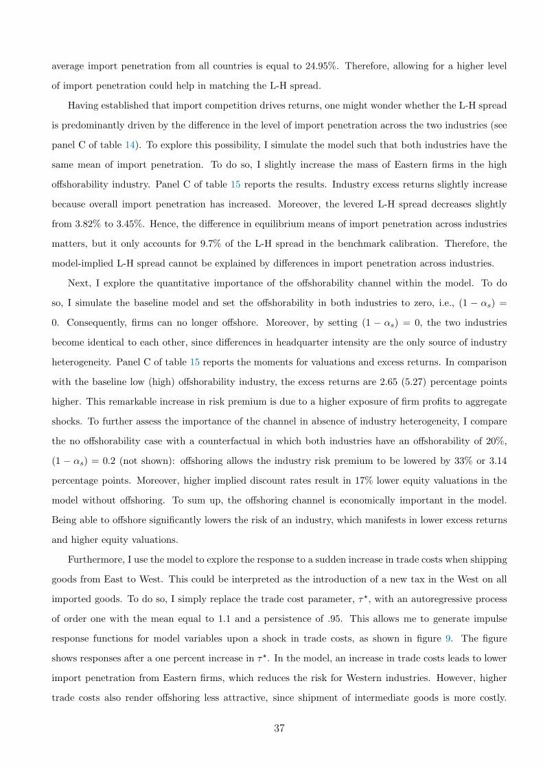
average import penetration from all countries is equal to 24.95%. Therefore, allowing for a higher level

of import penetration could help in matching the L-H spread.

Having established that import competition drives returns, one might wonder whether the L-H spread

is predominantly driven by the difference in the level of import penetration across the two industries (see

panel C of table 14). To explore this possibility, I simulate the model such that both industries have the

same mean of import penetration. To do so, I slightly increase the mass of Eastern firms in the high

offshorability industry. Panel C of table 15 reports the results. Industry excess returns slightly increase

because overall import penetration has increased. Moreover, the levered L-H spread decreases slightly

from 3.82% to 3.45%. Hence, the difference in equilibrium means of import penetration across industries

matters, but it only accounts for 9.7% of the L-H spread in the benchmark calibration. Therefore, the

model-implied L-H spread cannot be explained by differences in import penetration across industries.

Next, I explore the quantitative importance of the offshorability channel within the model. To do

so, I simulate the baseline model and set the offshorability in both industries to zero, i.e., (1 − αs) =

0. Consequently, firms can no longer offshore. Moreover, by setting (1 − αs) = 0, the two industries

become identical to each other, since differences in headquarter intensity are the only source of industry

heterogeneity. Panel C of table 15 reports the moments for valuations and excess returns. In comparison

with the baseline low (high) offshorability industry, the excess returns are 2.65 (5.27) percentage points

higher. This remarkable increase in risk premium is due to a higher exposure of firm profits to aggregate

shocks. To further assess the importance of the channel in absence of industry heterogeneity, I compare

the no offshorability case with a counterfactual in which both industries have an offshorability of 20%,

(1 − αs) = 0.2 (not shown): offshoring allows the industry risk premium to be lowered by 33% or 3.14

percentage points. Moreover, higher implied discount rates result in 17% lower equity valuations in the

model without offshoring. To sum up, the offshoring channel is economically important in the model.

Being able to offshore significantly lowers the risk of an industry, which manifests in lower excess returns

and higher equity valuations.

Furthermore, I use the model to explore the response to a sudden increase in trade costs when shipping

goods from East to West. This could be interpreted as the introduction of a new tax in the West on all

imported goods. To do so, I simply replace the trade cost parameter, τ⋆, with an autoregressive process

of order one with the mean equal to 1.1 and a persistence of .95. This allows me to generate impulse

response functions for model variables upon a shock in trade costs, as shown in figure 9. The figure

shows responses after a one percent increase in τ⋆. In the model, an increase in trade costs leads to lower

import penetration from Eastern firms, which reduces the risk for Western industries. However, higher

trade costs also render offshoring less attractive, since shipment of intermediate goods is more costly.

37

Consistent with this, figure 9 shows that both import penetration and the fraction of firms that offshore

fall upon an increase in τ⋆. Interestingly, the asset prices of Western firms also decrease in the model.

Hence, the reduction in the benefits from offshoring outweigh the positive effects from lower import

penetration. Consistent with this, asset prices drop more for the high compared to low offshorability

industry.

[Insert Figures 9 and 10 here.]

Finally, I explore through the lens of the model what would happen if the comparative cost advantage

of the East over the West were to fade away. This is an important counterfactual, given that hourly

manufacturing wages in China have risen by an average of 12% per year since 2001.79 In particular, I

assume that the comparative cost advantage of the East decreases to half of its initial magnitude. Figure

10 reports impulse responses to a positive productivity shock in the East, A⋆, for the benchmark and

the low comparative cost advantage economies. As the comparative advantage becomes smaller, the

East loses its relative cost competitiveness over the West. This leads to lower import penetration and

exposure of Western firms to aggregate productivity shocks in the East. As a result, industry profits and

asset prices drop less compared to the benchmark economy, and the unconditional risk premium is lower.

Importantly, the L-H spread is also smaller, with a low comparative advantage.80 Intuitively, offshoring

provides insurance against a risk that is less severe compared to the benchmark economy.

5 Conclusion

This paper studies how the possibility to relocate production affects industries’ cost of capital. Using a

new measure of offshorability at the industry level, I find that industries with low offshoring potential carry

an annualized 7.31 percent risk premium over industries with high offshoring potential. This suggests that

the option to offshore is an important driver of industry risk. The offshorability premium for services is

only half that of manufacturing. For manufacturing industries, traditional factor models fail to explain

the offshorability premium. For service industries, on the other hand, the premium is explained by the

CAPM and a positive loading on the U.S. market.

An explanation based on the recent surge in international trade and specialization is consistent with

various return patterns in the data. Intuitively, being able to reduce production costs through offshoring

allows firms to compete against foreign competitors from low-wage countries. Consistent with this, double

79 See the article “A tightening grip” in the Economist from March 12, 2015.80 The annualized market risk premium and the L-H spread in the low comparative advantage economy are equal

to 4.54% and 2.52%, respectively.

38

sorts of monthly excess returns on industry import penetration from low-wage countries and offshorability

show that the offshorability premium is increasing in import penetration from low-wage countries.

A two-country general equilibrium trade model that embeds the option to offshore is able to rationalize

a number of stylized facts: (1) there is a positive excess return spread between low and high offshora-

bility industries; (2) the offshorability spread is increasing in import penetration; (3) excess returns for

multinational companies are higher than for domestic firms; and (4) industry excess returns are increas-

ing in import penetration. Moreover, within the model, counterfactuals indicate that the offshorability

channel is economically important, as it allows industries to lower risk premia by 33% and increase equity

valuations by 17%.

Importantly, three main model predictions are strongly supported by the data. First, the model

predicts a negative relationship between offshorability and profit volatility. In the data, a one standard

deviation increase in industry offshorability is associated with an up to 19.7% lower profit volatility for the

median firm. Second, the model predicts that the offshorability premium is the largest in industries that

have high elasticities of substitution with respect to imported goods. Double sorts of monthly industry

excess returns on U.S. trade elasticities and offshorability confirm this prediction. Finally, within the

model, low (high) offshorability industries have high (low) covariance with consumption. Consistent with

this, I find that the strategy which is long low and short high offshorability industries has a positive and

significant consumption beta in the data.

Finally, the model implies that a sudden tax increase on all imported goods results in a decrease in

consumption and asset prices. Put differently, losing access to international specialization and offshoring

benefits outweighs the benefits from lower import competition.

39

References

Acemoglu, D., and D. H. Autor (2011): “Skills, tasks and technologies: Implications for employmentand earnings,” Handbook of Labor Economics, 4, 1043–1171.

Acemoglu, D., D. H. Autor, D. Dorn, G. H. Hanson, and B. Price (2016): “Import Competitionand the Great U.S. Employment Sag of the 2000s,” jole, 34, S141–S198.

Ahearne, A. G., W. L. Griever, and F. E. Warnock (2004): “Information costs and home bias:an analysis of U.S. holdings of foreign equities,” Journal of Interantional Economics, 62, 313–336.

Amiti, M., M. Dai, R. C. Feenstra, and J. Romalis (2016): “How Did China’s WTO Entry BenefitUS Consumers,” Working Paper.

Amiti, M., and S.-J. Wei (2009): “Service Offshoring and Productivity: Evidence from the US,” The

World Economy, 32, 203–220.

Antras, P. (2015): Global Production: Firms, Contracts, and Trade Structure. Princeton UniversityPress, 5 edn.

Antras, P., T. C. Fort, and F. Tintelnot (2016): “The Margins of Global Sourcing: Theory andEvidence from U.S. Firms,” Working Paper.

Antras, P., and E. Helpman (2004): “Global Sourcing,” Journal of Political Economy, 112, 552–580.

Atalay, E., A. Hortacsu, and C. Syverson (2013): “Vertical Integration and Input Flows,” Amer-

ican Economic Review, 104, 1120–1148.

Autor, D. H., D. Dorn, and G. H. Hanson (2013): “The Cina Syndrome: Local Labor MarketEffects of Import Competition in the United States,” American Economic Review, 103, 2121–2168.

(2016): “The China Shock: Learning from Labor Market Adjustment to Large Changes inTrade,” Annual Review of Economics, forthcoming.

Bandi, F. M., and A. Tamoni (2017): “The horizon of systematic risk: a new beta representation,”Working Paper.

Bansal, R., and A. Yaron (2004): “Risks for the Long Run: A Potential Resolution of Asset PricingPuzzles,” Journal of Finance, 59, 1481–1509.

Barrot, J.-N., E. Loualiche, and J. Sauvagnat (2017): “The Globalization Risk Premium,” Work-ing Paper.

Belo, F., X. Lin, J. Li, and X. Zhao (2015): “Labor-Force Heterogeneity and Asset Prices: theImportance of Skilled Labor,” Working Paper.

Bernard, A. B., J. B. Jensen, J. Eaton, and S. Kortum (2003): “Plants and Productivity inInternational Trade,” American Economic Review, 21, 105–130.

Bernard, A. B., J. B. Jensen, S. J. Redding, and P. K. Schott (2016): “Global Firms,” NBERWorking Paper No. 22727.

Bernard, A. B., J. B. Jensen, and P. K. Schott (2006a): “Survival of the Best Fit: Low WageCompetition and the (Uneven) Growth of Manufacturing Plants,” Journal of Interantional Economics,68, 219–237.

(2006b): “Trade Costs, Firms and Productivity,” Journal of Monetary Economics, 53, 917–937.

Blinder, A. S. (2009): “How Many U.S. Jobs Might Be Offshorable,” World Economics, 10, 41–78.

40

Bloom, N., M. Draca, and J. Van Reenen (2015): “Trade Induced Technical Change: The Impactof Chinese Imports on Innovation, Diffusion and Productivity,” Review of Economic Studies, pp. 1–33.

Brainard, W. C., W. R. Nelson, and M. D. Shapiro (1991): “The Consumption Beta ExplainsExpected Returns at Long Horizons,” Manuscript, Economics Department, Yale University.

Breeden, D. T., M. R. Gibbons, and R. H. Litzenberger (1989): “Empirical Tests of theConsumption-Oriented CAPM,” Journal of Finance, 44, 231–62.

Bretscher, L., C. Julliard, and C. Rosa (2016): “Human Capital and International PortfolioDiversification: A Reappraisal,” Journal of Interantional Economics, 99, 78–99.

Broda, C., and D. E. Weinstein (2006): “Globalization and the Gains From Variety,” Quarterly

Journal of Economics, 121, 541–585.

Bustamante, M. C., and A. Donangelo (2016): “Product market competition and industry returns,”Review of Financial Studies, forthcoming.

Campbell, J. Y. (1996): “Understanding Risk and Return,” Journal of Political Economy, 104, 298–345.

Carhart, M. M. (1997): “On persistence in mutual fund performance,” Journal of Finance, 52, 57–82.

Chaney, T. (2008): “Distorted Gravity: The Intensive and Extensive Margins of International Trade,”American Economic Review, 98, 1707–1721.

Chen, C., and C. Steinwender (2016): “Import Competition, Heterogenous Preferences of Managersand Productivity,” Working Paper.

Cochrane, J. H. (1996): “A Cross-Sectional Test of an Investment-Based Asset Pricing Model,” Journal

of Political Economy, 104, 572–621.

Coeurdacier, N., and H. Rey (2012): “Home Bias in Open Economy Financial Macroecnomics,”Journal of Economic Literature, 51, 63–115.

Corhay, A., H. Kung, and L. Schmid (2017): “Competition, markups, and predictable returns,”Working Paper.

Coval, J. D., and T. J. Moskowitz (1999): “Home Bias at Home: Local Equity Preference inDomsetic Portfolios,” Journal of Finance, 54, 2045–2073.

Danthine, J.-P., and J. B. Donaldson (2002): “Labour Relations and Asset Returns,” Review of

Economic Studies, 69, 41–64.

Dixit, A. K., and J. E. Stiglitz (1977): “Monopolistic Competition and Optimum Product Diversity,”American Economic Review, 67, 297–308.

Donangelo, A. (2014): “Labor Mobility: Implications for Asset Pricing,” Journal of Finance, 68,1321–1346.

Donangelo, A., F. Gourio, M. Kehrig, and M. Palacios (2016): “The Cross-Section of LaborLeverage and Equity Returns,” Working Paper.

Ebenstein, A., A. Harrison, M. McMillan, and S. Phillips (2014): “Why are American Work-ers Getting Poorer? Estimating the Impact of Trade and Offshoring Using the Current PopulationSurveys,” Review of Economics and Statistics, 96, 581–595.

Eisfeldt, A. L., and D. Papanikolaou (2013): “Organization capital and the cross-section of expectedreturns,” Journal of Finance, 68, 1365–1406.

41

Fama, E. F., and K. R. French (1992): “The cross-section of expected stock returns,” Journal of

Finance, 47, 427–465.

(2015): “A five-factor asset pricing model,” Journal of Financial Economics, 116, 1–22.

Favilukis, J., and X. Lin (2016): “Wage Rigidity: A Quantitative Solution to Several Asset PricingPuzzles,” Review of Financial Studies, 29, 148–192.

Fillat, J. L., and S. Garetto (2015): “Risk, Returns, and Multinational Production,” Quarterly

Journal of Economics, 130, 2027–2073.

Firpo, S., N. Fortin, and T. Lemieux (2013): “Occupational Tasks and Changes in the Wage Struc-ture,” Working Paper.

French, K. R., and J. M. Poterba (1991): “Investor Diversification and International Equitiy Mar-kets,” American Economic Review, 81, 222–226.

Fresard, L. (2010): “Financial Strength and Product Market Behavior: The Real Effects of CorporateCash Holdings,” Journal of Finance, 65, 61097–1122.

Fresard, L., and P. Valta (2016): “How Does Corporate Investment Respond to Increased EntryThreat?,” Review of Corporate Finance Studies, 5, 1–35.

Gabaix, X., and D. Laibson (2002): “The 6D Bias and the Equity Premium Puzzle,” in N.B.E.R.

Macroeconomics Annual 2001, ed. by B. Bernanke, and K. Rogoff, pp. 257–312. Cambridge: MIT Press.

Ghironi, F., and M. Melitz (2005): “International Trade and Macroeconomic Dynamics with Het-erogenous Firms,” Quarterly Journal of Economics, 120, 865–915.

Glassman, D. A., and L. A. Riddick (2001): “What causes home asset bias and how should it bemeasured,” Journal of Empirical Finance, 8, 35–54.

Gomes, J., U. Jermann, and L. Schmid (2017): “Sticky Leverage,” American Economic Review,forhcoming.

Goos, M., and A. Manning (2007): “Lousy and Lovely Jobs: The Rising Polarization of Work inBritain,” Review of Economic Studies, 89, 118–133.

Goos, M., A. Manning, and A. Salomons (2010): “Recent Changes in European EmploymentStructure: The Roles of Technological Change, Globalization and Institutions,” Working Paper.

Gourio, F. (2007): “Labor leverage, firms’ heterogeneous sensitivities to the business cycle, and thecross-section of expected returns,” Working Paper.

Hansen, P. (2005): “A test for superior predictive ability,” Journal of Business and Economic Statistics,23, 365–380.

Harrison, A., and M. McMillan (2011): “Offshoring Jobs? Multinational and U.S. ManufacturingEmployment,” Review of Economic Studies, 93, 857–875.

Heckscher, E. (1919): “The Effect of Foreign Trade on the Distribution of Income,” Ekonomisk Tid-

skrift, pp. 497–512.

Hombert, J., and A. Matray (2017): “Can Innovation Help U.S. Manufacturing Firms Escape ImportCompetition from China?,” Working Paper.

Hummels, D. (2007): “Transportation Costs and International Trade in the Second Era of Globalization,”Journal of Economic Perspectives, 21, 131–154.

42

Hummels, D., R. Jørgensen, J. R. Munch, and C. Xiang (2016): “The Wage Effects of Offshoring:Evidence from Danish Matched Worker-Firm Data,” American Economic Review, 104, 1597–1629.

Jensen, B. J. (2011): Global Trade in Services: Fear, Facts, and Offshoring. Peterson Institute ForInternational Economics, 1 edn.

Jensen, B. J., and L. G. Kletzer (2010): “Measuring Tradeable Services and the Task Contentof Offshorable Services Jobs,” in Labor in the New Economy, ed. by K. Abraham, M. Harper, andJ. Spletzer, pp. 309–335. University of Chicago Press.

King, M., S. Ruggles, J. T. Alexander, S. Flood, K. Genadek, M. B. Schroeder, B. Trampe,

and R. Vick (2010): “Integrated Public Use Microdata Series, Current Population Survey: Version3.0,” Minnesota Population Center, Minneapolis.

Kuehn, L.-A., M. Simutin, and J. J. Wang (2017): “A labor capital asset pricing model,” Journal

of Finance.

Lettau, M., and S. Ludvigson (2001): “Resurrecting the (C)CAPM: A Cross-Sectional Test WhenRisk Premia Are Time-Varying,” Journal of Political Economy, 109, 1238–1287.

Loualiche, E. (2015): “Asset Pricing with Entry and Imperfect Competition,” Working Paper.

Lustig, H., N. Roussanov, and A. Verdelhan (2011): “Common Risk Factors in Currency Markets,”Review of Financial Studies, 24, 3731–3777.

Lynch, A. (1996): “Decision Frequency and Synchronization across Agents: Implications for AggregateConsumption and Equity Returns,” Journal of Finance, 51, 1479–1497.

Magyari, I. (2017): “Firm Reorganization, Chinese Imports, and US Manufacturing Employment,”Working Paper.

Mankiw, G. N., and M. D. Shapiro (1986): “Risk and Return: Consumption Beta versus MarketBeta,” Review of Economics and Statistics, 68, 452–459.

Marshall, D., and N. Parekh (1999): “Can Costs of Consumption Adjustment Explain Asset PricingPuzzles?,” Journal of Finance, 54, 623–654.

Melitz, M. (2003): “The Impact of Trade on Intra-Industry Reallocations and Aggregate IndustryProductivity,” Econometrica, 71, 1695–1725.

Minton, B. A., and C. Schrand (1999): “The impact of cash flow volatility on discretionary investmentand the cost of debt and equity financing,” Journal of Financial Economics, 54, 423–460.

Nieuwerburgh, S. V., and L. Veldkamp (2009): “Information Immobility and the Home Bias Puz-zle,” Journal of Finance, 64, 1187–1215, 2009.

Novy-Marx, R. (2011): “Operating leverage,” Review of Finance, 15, 103–134.

Ochoa, M. J. (2013): “Volatility, Labor Heterogeneity and Asset Prices,” Working Paper.

Ohlin, B. (1933): Interregional and International Trade. Camebridge, MA: Harvard University Press.

Parker, J., and C. Julliard (2005): “Consumption Risk and the Cross-Section of Expected Returns,”Journal of Political Economy, 113, 185–222.

Patton, A. J., and A. Timmermann (2010): “Monotonicity in asset returns: New tests with appli-cations to the term structure, the CAPM, and portfolio sorts,” Journal of Financial Economics, 98,605–625.

43

Pierce, J., and P. Schott (2016): “The Surprisingly Swift Decline of U.S. Manufacturing Employ-ment,” American Economic Review, 106, 1632–1662.

Ramondo, N., V. Rappoport, and K. Ruhl (2016): “Intrafirm Trade and Vertical Fragmentation inU.S. Multinational Corporations,” Journal of Interantional Economics, 98, 51–59.

Ricardo, D. (1821): On the Principles of Political Economy and Taxation. London: John Murray, 3rdedition edn.

Romano, J., and M. Wolf (2005): “Stepwise multiple testing as formalized data snooping,” Econo-

metrica, 73, 1237–1282.

Schott, P. (2008): “The Relative Sophistication of Chinese Exports,” Economic Policy, 53, 5–49.

Tuzel, S., and M. B. Zhang (2017): “Local risk, local factors, and asset prices,” Journal of Finance,72, 325–370.

Valta, P. (2012): “Competition and the Cost of Debt,” Journal of Financial Economics, 105, 661–682.

Verdelhan, A. (2017): “The Share of Sytematic Variation in Bilateral Exchange Rates,” Journal of

Finance, forhcoming.

Xu, J. (2012): “Understanding China’s growth: Past, present, and future,” Journal of Economic Per-

spectives, 106, 427–446.

Zhang, M. B. (2016): “Labor-Technology Substitution: Implications for Asset Pricing,” Working Paper.

44

Appendix

A Model

A.1 Demand Side

1st Layer - Sector Demand

In the first layer, households decide how to optimally allocate consumption between homogenous anddifferentiated goods:

maxc1−a00 Ca0T , s.t. PTCT + p0c0 ≤ Y,

where CT is the consumption index aggregated from consumption in the S industries consisting of dif-ferentiated goods, PT is the corresponding price index, c0 and p0 are the consumption and price of thehomogenous good, and Y is the total income of consumers. First-order conditions imply the followingdemand functions and the aggregate price index, P :

c0 = (1− a0)PC

p0

CT = a0PC

PT

P =

(PTa0

)a0 ( p01− a0

)1−a0

The good 0 is produced under constant returns to scale and a production function that is linear inlabor.81 Moreover, the good is freely traded and used as a numeraire in each country. Its price is set to1.82 Consequently, productivity changes across countries can be interpreted as real productivity changes.

2nd Layer - Industry Demand

The aggregation over industry consumption is constant elasticity of substitution with elasticity θ. Theoptimization problem is as follows:

max

[∑

s

δ1θs C

θ−1θ

s

] θθ−1

, s.t.∑

s

PsCs ≤ PTCT ,

where Ps are industry price levels and ηs are industry taste parameters such that∑

s ηs = 1. First-orderconditions imply demand functions and price indices:

Cs = δs

(PsPT

)−θ

CT

PT =

[∑

s

δsP1−θs

] 11−θ

3rd Layer - Product Demand

Demand for the product variety, ω, produced by firms:

cs(ϕ) =

(ps(ϕ)

Ps

)−σs

Cs

81 In other words, one unit of labor produces one unit of good 0.82 This normalization also leads to wages being equal to 1 in both countries.

45

Price index in industry s:

Ps =

[∫

Ωs

ps(ϕ)1−σsdϕ

] 11−σs

A.2 Aggregation - Western Firms

Domestic Production

The fraction of firms that choose not to offshore is:

ζs,D = Probϕ < ϕs,O = G(ϕs,O) = 1−

(ϕs,Oϕmin

)−κs

The average productivity of firms with productivity higher than the minimum productivity ϕs,min butlower than the cutoff value ϕs,O is equal to:

ϕs,D =

[∫ ϕs,Oϕs,min

ϕσs−1dGs(ϕ)

G(ϕs,O)

] 1σs−1

= νs

ϕσs−1min − ϕκsminϕ

(σs−1)−kss,O

1−(ϕs,minϕs,O

)ks

1σs−1

where νs =[

κsks−(σs−1)

] 1σs−1

.

Partially Offshored Firms

The fraction of firms that choose to offshore is:

ζs,O = Probϕ > ϕs,O = 1−G(ϕs,O) =

(ϕs,Oϕs,min

)−κs

The average productivity of firms with productivity higher than cutoff value ϕs,O is equal to:

ϕs,O =

[∫∞

ϕs,Oϕσs−1dGs(ϕ)

1−G(ϕs,O)

] 1σs−1

= νsϕs,O

Export: Partially Offshored Firms

This is the relevant case for firms with headquarter in the West. The average productivity of firms withproductivity higher than the cutoff ϕs,X,O is equal to:

ϕs,X,O =

[∫∞

ϕs,X,Oϕσs−1dGs(ϕ)

1−G(ϕs,X,O)

] 1σs−1

= νsϕs,X,O

The fraction of firms that choose to offshore is:

ζs,X,O = Probϕ > ϕs,X,O = 1−G(ϕs,X,O) =

(ϕs,X,Oϕs,min

)−κs

A.3 Aggregation - Eastern Firms

Domestic Production

All firms engage in domestic production. Hence, the fraction is equal to 1. The average productivityof firms with productivity higher than the minimum productivity ϕs,min but lower than the cutoff value

46

ϕs,O is equal to:

ϕ⋆s,D =

[∫

∞

ϕ⋆s,min

ϕσs−1dGs(ϕ)

] 1σs−1

= νsϕ⋆s,min

Export: Purely Domestic Firms

The fraction of firms that choose to export is:

ζ⋆s,X,D = Probϕ > ϕ⋆s,X,D = 1−G(ϕ⋆s,X,D) =

(

ϕ⋆s,X,Dϕ⋆s,min

)−κs

The average productivity of firms with productivity higher than the cutoff ϕ⋆s,X,D is equal to:

ϕ⋆s,X,D =

∫∞

ϕ⋆s,X,D

ϕσs−1dGs(ϕ)

1−G(ϕ⋆s,X,D)

1σs−1

= νsϕ⋆s,X,D

A.4 Model Extension: International Bond Trading

In this section, I allow for international sovereign bond trading as in Ghironi and Melitz (2005). Allowingfor bond trading is an important model extension because it allows model households to smooth con-sumption intertemporally. In addition, introducing bonds allows one to study current accounts for thetwo countries in the model.

Households can trade bonds domestically and internationally. Western (Eastern) bonds are issued byWestern (Eastern) households and denominated in Western (Eastern) currency. Hence, bonds issued byeach country provide a risk-free real return in units of that country’s consumption basket. Internationalasset markets, however, are incomplete, as only risk-free bonds are traded across countries. This wouldimply indeterminacy of steady-state net foreign assets and non-stationarity. As a remedy, I assume thatagents must pay a convex adjustment cost when adjusting their bond holdings, which can be interpretedas a fee paid to financial intermediaries. This is sufficient to uniquely pin down the steady state, and itleads to stationary dynamics of responses to shocks.

Additional Model Equations

Bond trading affects the households’ budget constraints, which become

PtQD,t+1+PtFtQX,t+1 + Ptξ

2Q2D,t+1 + Pt

ξ

2FtQ

2X,t+1 + PtCt

≤ (1 + rf,t)PtQD,t + (1 + r⋆f,t)FtPtQX,t+1 + T ft +Πt(α)

P ⋆t Q⋆D,t+1+P

⋆t

Q⋆X,t+1

Ft+ P ⋆t

ξ

2

(Q⋆D,t+1

)2+ P ⋆t

ξ

2

(

Q⋆X,t+1

)2

Ft+ P ⋆t C

⋆t

≤ (1 + r⋆f,t)P⋆t Q

⋆D,t + (1 + rf,t)P

⋆t

Q⋆X,t+1

Ft+ T ⋆,ft +Π⋆t (α),

where Ft =P ⋆tPt

denotes the real exchange rate, QD,t+1 (QX,t+1) denote Western households’ bond holdings

of the Western (Eastern) bond, (ξ/2)Q2D,t+1 is the cost of adjusting holdings of the Western bonds,

(ξ/2)FtQ2X,t+1 is the cost of adjusting holdings of the Eastern bonds and T ft is the fee rebate, taken

as given by the household (note T ft = (ξ/2)[

FtQ2X,t+1 + FtQ

2X,t+1

]

in equilibrium). Symmetry implies

analogous equations for Eastern quantities. For simplicity, I assume that the cost parameter ξ is identicalfor Western and Eastern bonds and set it to a value of 0.0025, as in Ghironi and Melitz (2005).

47

Western and Eastern households maximize their respective intertemporal utility functions subject tothe respective constraints. Taking first-order conditions leads to two Euler equations for the risk-free ratein each country:

1 + ξQD,t+1 = (1 + rf,t+1)E [Mt,t+1]

1 + ξQX,t+1 =(1 + r⋆f,t+1

)E

[

Mt,t+1Ft+1

Ft

]

1 + ξQ⋆D,t+1 =(1 + r⋆f,t+1

)E[M⋆t,t+1

]

1 + ξQ⋆X,t+1 = (1 + rf,t+1)E

[

M⋆t,t+1

FtFt+1

]

The terms related to the stock of bonds on the left-hand side of the Euler equations are key for determinacyof the steady state and model stationarity. Basically, they ensure that zero holdings of bonds are theunique steady state in which the product of the SDF and the gross interest rate equals one in each countrysuch that the economy returns to this initial position after temporary shocks.

Moreover, equilibrium requires that Western and Eastern bonds be in global zero net supply:

QD,t+1 +Q⋆X,t+1 = 0

Q⋆D,t+1 +QX,t+1 = 0

Lastly, current accounts can be introduced to the model. Current accounts are, by definition, equalto the changes in aggregate bond holdings in the two countries:

CAt = QD,t+1 −QD,t + Ft (QX,t+1 −QX,t)

CA⋆t = Q⋆D,t+1 −Q⋆D,t +Q⋆X,t+1 −Q⋆X,t

Ft

The global zero net supply conditions for the bond market imply that a country’s borrowing must equalthe other country’s lending, CAt + FtCA

⋆t = 0.

Table A1 reports the results for model simulations with international bond trading. Not surprisingly,the standard deviation of consumption decreases compared to the baseline model, as bonds allow house-holds to smooth their consumption intertemporally. This also leads to a lower overall risk premium, whichcan be seen from the lower mean of industry excess returns. Importantly, however, the L-H spread isunaffected by the introduction of international bond trading. Effectively, trading risk-free bonds allowshouseholds to transfer consumption across time in a state- and industry-independent manner, which doesnot help mitigate industry-specific exposure to aggregate shocks.

Similar to table 15, Panels C and D of table A1 report the moments related to the two shocks in themodel. Also, after introducing bond trading to the model, shocks to A⋆ make up for roughly 88% of theL-H spread.

Finally, the model with sovereign bonds allows one to examine how productivity shocks affect thebalance of current accounts in each country. Figure A1 reports impulse response functions of CAt andCA⋆t to productivity shocks in the West (first row) and East (second row). As in Ghironi and Melitz (2005),positive productivity shocks in the East (West) are associated with increases (decreases) in consumption,which leads to a current account surplus (deficit) in the East and a current account deficit (surplus) inthe West.

48

A.5 Elasticities

Elasticities related to total, sector and industry consumption:

η⋆ (C) = −η⋆ (P ) +Π

L+Πη⋆ (Π)

η⋆ (CT ) = η⋆ (C)− (1− a0) η⋆ (PT ) = η⋆ (C)−

(1

a0− 1

)

η⋆ (P )

η⋆ (Cs) = −θη⋆ (Ps) + θη⋆ (PT ) + η⋆ (CT ) = −θη⋆ (Ps) + η⋆ (C) + [θ − (1− a0)] η⋆ (PT )

Elasticities related to total and sector price indices:

η⋆ (P ) = a0η⋆ (PT )

η⋆ (PT ) =∑

S

δs

(PTPs

)θ−1

η⋆ (Ps)

Elasticities related to offshoring and exporting cutoffs and fractions:

η⋆ (ζs,O) = −κsη⋆ (ϕs,O)

η⋆ (ϕs,O) = η⋆ (ϕs,O)

η⋆ (ζs,X,O) = −κsη⋆ (ϕs,X,O)

η⋆ (ϕs,X,O) = η⋆ (ϕs,X,O)

The elasticity of total industry profits is driven by the elasticities of domestic profits and profits fromexports:

η⋆ (Π) = η⋆(ΠD)+ η⋆

(ΠX)

Elasticity of total domestic profits:

η⋆(ΠD)

= − (σs − θ) (−η⋆ (Ps))︸ ︷︷ ︸

competition effect

+ η⋆ (Cs) +1− a0 − θ

a0(−η⋆ (P ))

︸ ︷︷ ︸

expenditure effect

+

κsζs,O (πs,O − πs,D)

ΠD︸ ︷︷ ︸

relative benefits from offshoring

− (σs − 1)ζs,Dπs,DΦ+ ζs,Oπs,O

ΠD︸ ︷︷ ︸

industry composition effect

(−η⋆ (ϕs,O)) +

ζs,Oπs,OΠD

(σs − 1) (1− αs)︸ ︷︷ ︸

productivity gain from offshoring

where

Φ =ϕκss,minσs − 1

ϕσs−κss,O [κs − (σs − 1)]

ϕσs−1s,min − ϕκss,min

1

ϕκs−(σs−1)s,O

−κs

ϕκss,O − ϕκss,min

and Φ > 0 and ∂Φ∂ϕs,O

> 0. This means that the negative response of domestic profits after a shock

to A⋆ is more pronounced when fewer firms offshore. This result is intuitive, since firms that offshoredirectly profit from the increase in productivity, which makes them more resistant against increases incompetition.

49

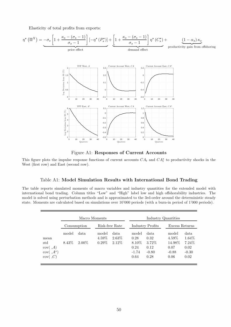
Elasticity of total profits from exports:

η⋆(ΠX)= −σs

[

1 +κs − (σs − 1)

σs − 1

]

[−η⋆ (P ⋆s )]

︸ ︷︷ ︸

price effect

+

[

1 +κs − (σs − 1)

σs − 1

]

η⋆ (C⋆s )

︸ ︷︷ ︸

demand effect

+ (1− αs) κs︸ ︷︷ ︸

productivity gain from offshoring

0 10 20 30 400

0.5

1

1.5

2

LogDeviationfrom

SS(%

)

TFP West, A

0 10 20 30 40-0.1

0

0.1

0.2

0.3Current Account West, CA

0 10 20 30 40-0.6

-0.4

-0.2

0

0.2Current Account East, CA⋆

0 10 20 30 40Quarters

1

2

3

4

5

6

LogDeviationfrom

SS(%

)

TFP East, A⋆

0 10 20 30 40Quarters

-0.5

-0.4

-0.3

-0.2

-0.1

0

0.1Current Account West, CA

0 10 20 30 40Quarters

0

0.2

0.4

0.6

0.8

1

1.2Current Account East, CA⋆

Figure A1: Responses of Current Accounts

This figure plots the impulse response functions of current accounts CAt and CA⋆t to productivity shocks in the

West (first row) and East (second row).

Table A1: Model Simulation Results with International Bond Trading

The table reports simulated moments of macro variables and industry quantities for the extended model withinternational bond trading. Column titles “Low” and “High” label low and high offshorability industries. Themodel is solved using perturbation methods and is approximated to the 3rd-order around the deterministic steadystate. Moments are calculated based on simulations over 10’000 periods (with a burn-in period of 1’000 periods).

Macro Moments Industry Quantities

Consumption Risk-free Rate Industry Profits Excess Returns

model data model data model data model datamean 4.59% 2.63% 0.28 0.32 4.59% 1.64%std 8.43% 2.00% 0.29% 2.12% 8.10% 3.72% 14.98% 7.24%cov( ,A) 0.24 0.12 0.07 0.02cov( ,A⋆) -1.74 -0.80 -0.88 -0.30cov( ,C) 0.64 0.28 0.06 0.02

50

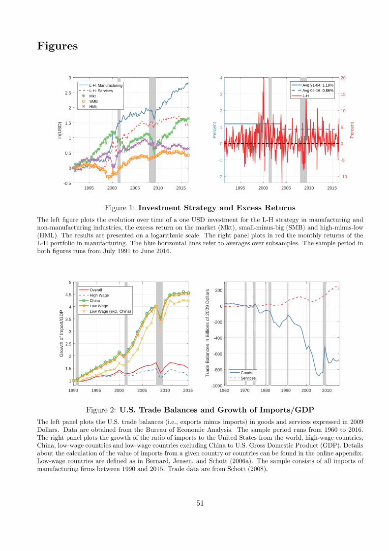
Figures

1995 2000 2005 2010 2015-0.5

0

0.5

1

1.5

2

2.5

3

ln(U

SD

)

L-H: ManufacturingL-H: ServicesMktSMBHML

1995 2000 2005 2010 2015

-2

-1

0

1

2

3

4

Per

cent

-10

-5

0

5

10

15

20

Per

cent

Avg 91-04: 1.19%Avg 04-16: 0.86%L-H

Figure 1: Investment Strategy and Excess Returns

The left figure plots the evolution over time of a one USD investment for the L-H strategy in manufacturing andnon-manufacturing industries, the excess return on the market (Mkt), small-minus-big (SMB) and high-minus-low(HML). The results are presented on a logarithmic scale. The right panel plots in red the monthly returns of theL-H portfolio in manufacturing. The blue horizontal lines refer to averages over subsamples. The sample period inboth figures runs from July 1991 to June 2016.

1960 1970 1980 1990 2000 2010-1000

-800

-600

-400

-200

0

200

Tra

de B

alan

ces

in B

illio

ns o

f 200

9 D

olla

rs

GoodsServices

1990 1995 2000 2005 2010 2015

1

1.5

2

2.5

3

3.5

4

4.5

5

Gro

wth

of I

mpo

rt/G

DP

OverallHigh WageChinaLow WageLow Wage (excl. China)

Figure 2: U.S. Trade Balances and Growth of Imports/GDP

The left panel plots the U.S. trade balances (i.e., exports minus imports) in goods and services expressed in 2009Dollars. Data are obtained from the Bureau of Economic Analysis. The sample period runs from 1960 to 2016.The right panel plots the growth of the ratio of imports to the United States from the world, high-wage countries,China, low-wage countries and low-wage countries excluding China to U.S. Gross Domestic Product (GDP). Detailsabout the calculation of the value of imports from a given country or countries can be found in the online appendix.Low-wage countries are defined as in Bernard, Jensen, and Schott (2006a). The sample consists of all imports ofmanufacturing firms between 1990 and 2015. Trade data are from Schott (2008).

51

ϕ(σ−1)D

5 10 ϕ(σ−1)O ϕ

(σ−1)X,O

25 ϕ(σ−1)X,D

ϕ(σ−1)

-4

-3

-2

-1

0

1

2

3

4

5

6

prof

itsπ

D

πO

πX,D

πX,O

ϕ(σ−1)D

2 ϕ(σ−1)X,D

6 ϕ(σ−1)X,O

10 12

ϕ(σ−1)

-4

-2

0

2

4

6

8

10

12

prof

its

π*D

π*O

π*X,D

π*X,O

Figure 3: Profits for Different Organizational Choices

This figure plots the profits for different organizational choices against a transformation of idiosyncratic firm produc-tivity, ϕσ−1. This is convenient, given that firm profits are linear in ϕσ−1. The left panel plots profits for Westernfirms and the right panel profits for Eastern firms, assuming that the East has a comparative cost advantage inproducing offshorable tasks.

52

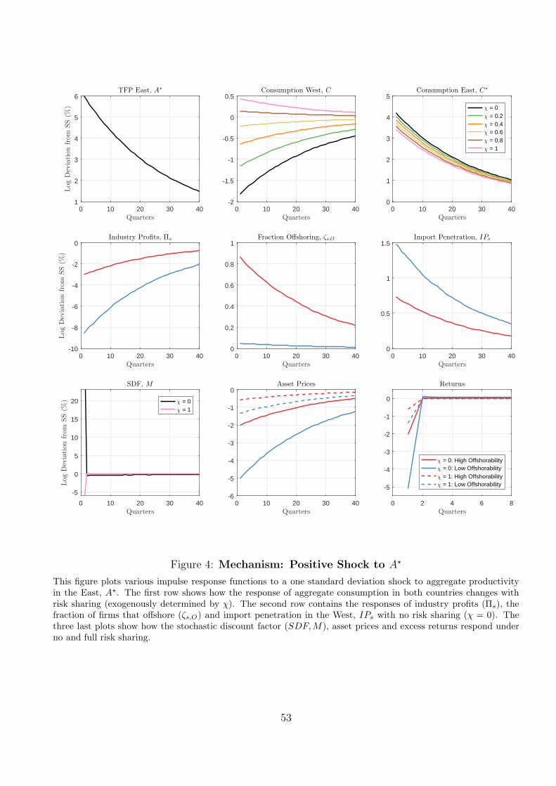
0 10 20 30 40Quarters

1

2

3

4

5

6

LogDeviationfrom

SS(%

)

TFP East, A⋆

0 10 20 30 40Quarters

-2

-1.5

-1

-0.5

0

0.5Consumption West, C

0 10 20 30 40Quarters

0

1

2

3

4

5Consumption East, C⋆

χ = 0χ = 0.2χ = 0.4χ = 0.6χ = 0.8χ = 1

0 10 20 30 40Quarters

-10

-8

-6

-4

-2

0

LogDeviationfrom

SS(%

)

Industry Profits, Πs

0 10 20 30 40Quarters

0

0.2

0.4

0.6

0.8

1Fraction Offshoring, ζs,O

0 10 20 30 40Quarters

0

0.5

1

1.5Import Penetration, IPs

0 10 20 30 40Quarters

-5

0

5

10

15

20

LogDeviationfrom

SS(%

)

SDF, M

χ = 0χ = 1

0 10 20 30 40Quarters

-6

-5

-4

-3

-2

-1

0Asset Prices

0 2 4 6 8Quarters

-5

-4

-3

-2

-1

0

Returns

χ = 0: High Offshorabilityχ = 0: Low Offshorabilityχ = 1: High Offshorabilityχ = 1: Low Offshorability

Figure 4: Mechanism: Positive Shock to A⋆

This figure plots various impulse response functions to a one standard deviation shock to aggregate productivityin the East, A⋆. The first row shows how the response of aggregate consumption in both countries changes withrisk sharing (exogenously determined by χ). The second row contains the responses of industry profits (Πs), thefraction of firms that offshore (ζs,O) and import penetration in the West, IPs with no risk sharing (χ = 0). Thethree last plots show how the stochastic discount factor (SDF,M), asset prices and excess returns respond underno and full risk sharing.

53

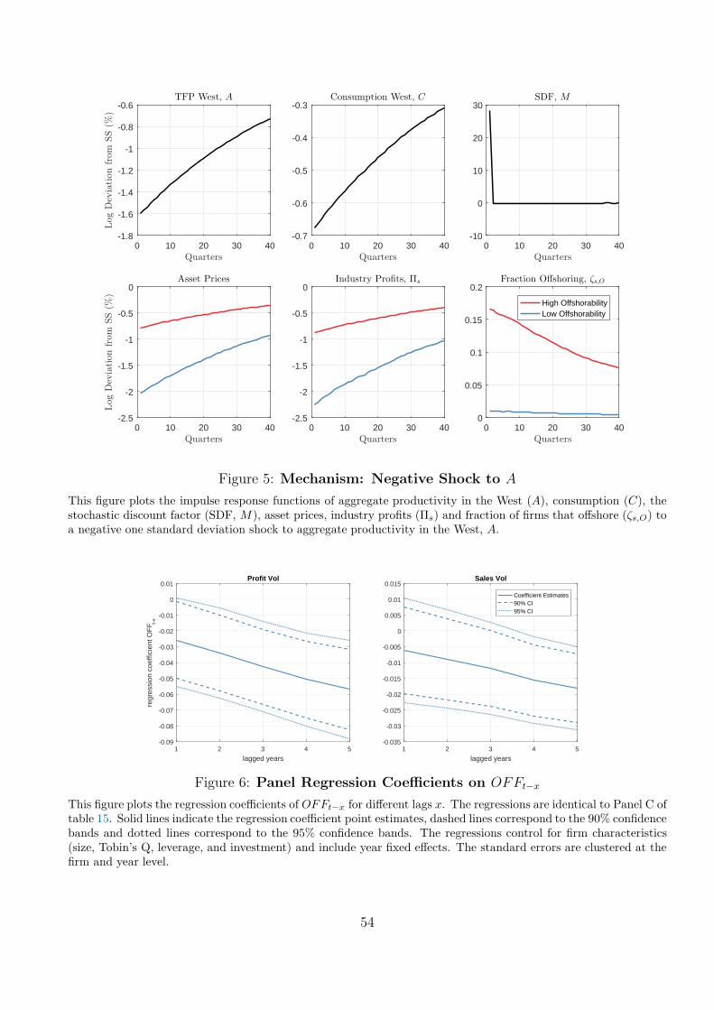
0 10 20 30 40Quarters

-1.8

-1.6

-1.4

-1.2

-1

-0.8

-0.6LogDeviationfrom

SS(%

)TFP West, A

0 10 20 30 40Quarters

-0.7

-0.6

-0.5

-0.4

-0.3Consumption West, C

0 10 20 30 40Quarters

-10

0

10

20

30SDF, M

0 10 20 30 40Quarters

-2.5

-2

-1.5

-1

-0.5

0

LogDeviationfrom

SS(%

)

Asset Prices

0 10 20 30 40Quarters

-2.5

-2

-1.5

-1

-0.5

0Industry Profits, Πs

0 10 20 30 40Quarters

0

0.05

0.1

0.15

0.2Fraction Offshoring, ζs,O

High OffshorabilityLow Offshorability

Figure 5: Mechanism: Negative Shock to A

This figure plots the impulse response functions of aggregate productivity in the West (A), consumption (C), thestochastic discount factor (SDF, M), asset prices, industry profits (Πs) and fraction of firms that offshore (ζs,O) toa negative one standard deviation shock to aggregate productivity in the West, A.

1 2 3 4 5

lagged years

-0.09

-0.08

-0.07

-0.06

-0.05

-0.04

-0.03

-0.02

-0.01

0

0.01

regr

essi

on c

oeffi

cien

t OF

F t-x

Profit Vol

1 2 3 4 5

lagged years

-0.035

-0.03

-0.025

-0.02

-0.015

-0.01

-0.005

0

0.005

0.01

0.015Sales Vol

Coefficient Estimates90% CI95% CI

Figure 6: Panel Regression Coefficients on OFFt−x

This figure plots the regression coefficients of OFFt−x for different lags x. The regressions are identical to Panel C oftable 15. Solid lines indicate the regression coefficient point estimates, dashed lines correspond to the 90% confidencebands and dotted lines correspond to the 95% confidence bands. The regressions control for firm characteristics(size, Tobin’s Q, leverage, and investment) and include year fixed effects. The standard errors are clustered at thefirm and year level.

54

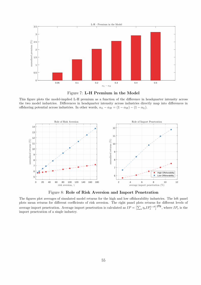
0.05 0.1 0.2 0.3 0.4 0.5αL − αH

0

0.5

1

1.5

2

2.5

3

3.5

annualizedpremium

(%)

L-H - Premium in the Model

Figure 7: L-H Premium in the Model

This figure plots the model-implied L-H premium as a function of the difference in headquarter intensity acrossthe two model industries. Differences in headquarter intensity across industries directly map into differences inoffshoring potential across industries. In other words, αL − αH = (1− αH)− (1− αL).

0 20 40 60 80 100 120 140 160 180risk aversion, γ

5

6

7

8

9

10

11

12

13

14

annualizedreturns(%

)

Role of Risk Aversion

2 4 6 8 10 12average import penetration (%)

6

7

8

9

10

11

12

annualizedreturns(%

)

Role of Import Penetration

High OffshorabilityLow Offshorability

Figure 8: Role of Risk Aversion and Import Penetration

The figures plot averages of simulated model returns for the high and low offshorability industries. The left panelplots mean returns for different coefficients of risk aversion. The right panel plots returns for different levels of

average import penetration. Average import penetration is calculated as IP =[∑

s ηsIP1−θs

] 11−θ , where IPs is the

import penetration of a single industry.

55

0 10 20 30 40Quarters

-0.2

-0.15

-0.1

-0.05

0Import Penetration, IPs

0 10 20 30 40Quarters

-0.1

-0.08

-0.06

-0.04

-0.02

0Fraction Offshoring, ζs,O

0 10 20 30 40Quarters

-0.25

-0.2

-0.15

-0.1

-0.05

0Asset Prices

High OffshorabilityLow Offshorability

Figure 9: Model Counterfactual: Shock to Variable Trade Costs τ ⋆

This figure plots the impulse response functions import penetration (IPs), fraction of firms that offshore (ζs,O) andasset prices to a positive one percent shock to variable trade costs (τ⋆).

0 10 20 30 40Quarters

-10

-8

-6

-4

-2

0

LogDeviationfrom

SS(%

)

Industry Profits, Πs

0 10 20 30 40Quarters

-6

-5

-4

-3

-2

-1

0Asset Prices

0 2 4 6 8Quarters

-6

-4

-2

0

2Returns

Benchmark: HLow CompAdv: HBenchmark: LLow CompAdv: L

Figure 10: Model Counterfactual: Benchmark vs Low Comparative Advantage

This figure plots the impulse response functions of industry profits (Πs), asset prices and industry excess returns toa positive one standard deviation shock to aggregate productivity in the East, A⋆. The solid lines are the impulseresponses in the benchmark economy, while the dashed lines correspond to impulse responses in an economy in whichthe comparative cost advantage in offshorable labor of the East is lower compared to the benchmark calibration.

56

Tables

Table 1: Occupation Tasks that define Offshorability

Panel A tabulates the tasks used to calculate occupation offshorability by Acemoglu and Autor (2011). Theacronyms WA and WC in the third column stand for work activity and work context. Panels B and C report thetop and bottom ten occupations by offshorability, offj.

Panel A: Acemoglu and Autor (2011)

4.C.1.a.2.l Face-to-Face Discussions WC4.A.4.a.5 Assisting and Caring for Others WA4.A.4.a.8 Performing for or Working Directly with the Public WA4.A.1.b.2 Inspecting Equipment, Structures, or Material WA4.A.3.a.2 Handling and Moving Objects WA4.A.3.b.4 Repairing and Maintaining Mechanical Equipment (*0.5) WA4.A.3.b.5 Repairing and Maintaining Electronic Equipment (*0.5) WA

Panel B: Top Ten Occupations by Offshorability

SOC Occupation Title offj

31-9094 Medical Transcriptionists 0.5041-9041 Telemarketers 0.4843-4011 Brokerage Clerks 0.4751-6021 Pressers, Textile, Garment, and Related Materials 0.4615-2041 Statisticians 0.4543-3031 Bookkeeping, Accounting, and Auditing Clerks 0.4543-9022 Word Processors and Typists 0.4551-6031 Sewing Machine Operators 0.4415-2099 Legal Support Workers 0.4415-1131 Computer Programmers 0.44

Panel C: Bottom Ten Occupations by Offshorability

SOC Occupation Title offj

37-3013 Tree Trimmers and Pruners 0.2647-4021 Elevator Installers and Repairers 0.2629-1151 Nurse Anesthetists 0.2629-1021 Dentists 0.2647-5013 Service Unit Operators, Oil, Gas, and Mining 0.2629-1024 Prosthodontists 0.2529-2041 Emergency Medical Technicians and Paramedics 0.2533-1021 Firefighters 0.2549-9051 Electrical Power-Line Installers and Repairers 0.2549-9095 Manufactured Building and Mobile Home Installers 0.24

57

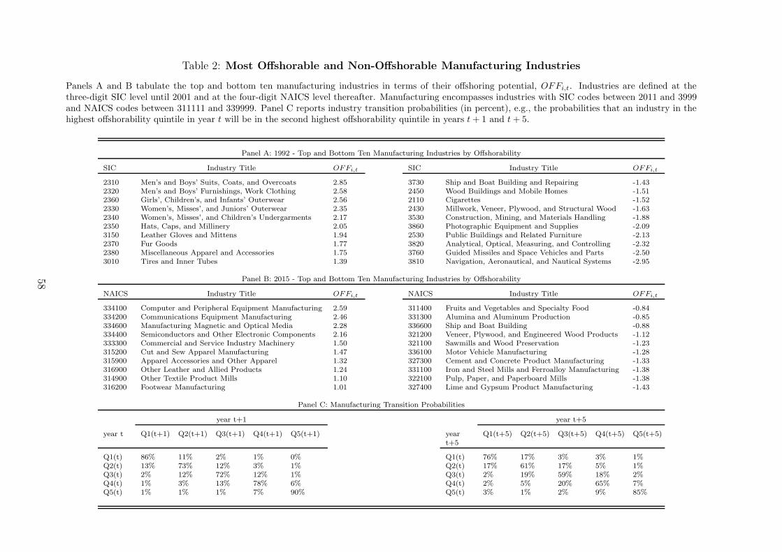
Table 2: Most Offshorable and Non-Offshorable Manufacturing Industries

Panels A and B tabulate the top and bottom ten manufacturing industries in terms of their offshoring potential, OFFi,t. Industries are defined at thethree-digit SIC level until 2001 and at the four-digit NAICS level thereafter. Manufacturing encompasses industries with SIC codes between 2011 and 3999and NAICS codes between 311111 and 339999. Panel C reports industry transition probabilities (in percent), e.g., the probabilities that an industry in thehighest offshorability quintile in year t will be in the second highest offshorability quintile in years t+ 1 and t+ 5.

Panel A: 1992 - Top and Bottom Ten Manufacturing Industries by Offshorability

SIC Industry Title OFFi,t SIC Industry Title OFFi,t

2310 Men’s and Boys’ Suits, Coats, and Overcoats 2.85 3730 Ship and Boat Building and Repairing -1.432320 Men’s and Boys’ Furnishings, Work Clothing 2.58 2450 Wood Buildings and Mobile Homes -1.512360 Girls’, Children’s, and Infants’ Outerwear 2.56 2110 Cigarettes -1.522330 Women’s, Misses’, and Juniors’ Outerwear 2.35 2430 Millwork, Veneer, Plywood, and Structural Wood -1.632340 Women’s, Misses’, and Children’s Undergarments 2.17 3530 Construction, Mining, and Materials Handling -1.882350 Hats, Caps, and Millinery 2.05 3860 Photographic Equipment and Supplies -2.093150 Leather Gloves and Mittens 1.94 2530 Public Buildings and Related Furniture -2.132370 Fur Goods 1.77 3820 Analytical, Optical, Measuring, and Controlling -2.322380 Miscellaneous Apparel and Accessories 1.75 3760 Guided Missiles and Space Vehicles and Parts -2.503010 Tires and Inner Tubes 1.39 3810 Navigation, Aeronautical, and Nautical Systems -2.95

Panel B: 2015 - Top and Bottom Ten Manufacturing Industries by Offshorability

NAICS Industry Title OFFi,t NAICS Industry Title OFFi,t

334100 Computer and Peripheral Equipment Manufacturing 2.59 311400 Fruits and Vegetables and Specialty Food -0.84334200 Communications Equipment Manufacturing 2.46 331300 Alumina and Aluminum Production -0.85334600 Manufacturing Magnetic and Optical Media 2.28 336600 Ship and Boat Building -0.88334400 Semiconductors and Other Electronic Components 2.16 321200 Veneer, Plywood, and Engineered Wood Products -1.12333300 Commercial and Service Industry Machinery 1.50 321100 Sawmills and Wood Preservation -1.23315200 Cut and Sew Apparel Manufacturing 1.47 336100 Motor Vehicle Manufacturing -1.28315900 Apparel Accessories and Other Apparel 1.32 327300 Cement and Concrete Product Manufacturing -1.33316900 Other Leather and Allied Products 1.24 331100 Iron and Steel Mills and Ferroalloy Manufacturing -1.38314900 Other Textile Product Mills 1.10 322100 Pulp, Paper, and Paperboard Mills -1.38316200 Footwear Manufacturing 1.01 327400 Lime and Gypsum Product Manufacturing -1.43

Panel C: Manufacturing Transition Probabilities

year t+1 year t+5

year t Q1(t+1) Q2(t+1) Q3(t+1) Q4(t+1) Q5(t+1) yeart+5

Q1(t+5) Q2(t+5) Q3(t+5) Q4(t+5) Q5(t+5)

Q1(t) 86% 11% 2% 1% 0% Q1(t) 76% 17% 3% 3% 1%Q2(t) 13% 73% 12% 3% 1% Q2(t) 17% 61% 17% 5% 1%Q3(t) 2% 12% 72% 12% 1% Q3(t) 2% 19% 59% 18% 2%Q4(t) 1% 3% 13% 78% 6% Q4(t) 2% 5% 20% 65% 7%Q5(t) 1% 1% 1% 7% 90% Q5(t) 3% 1% 2% 9% 85%

58

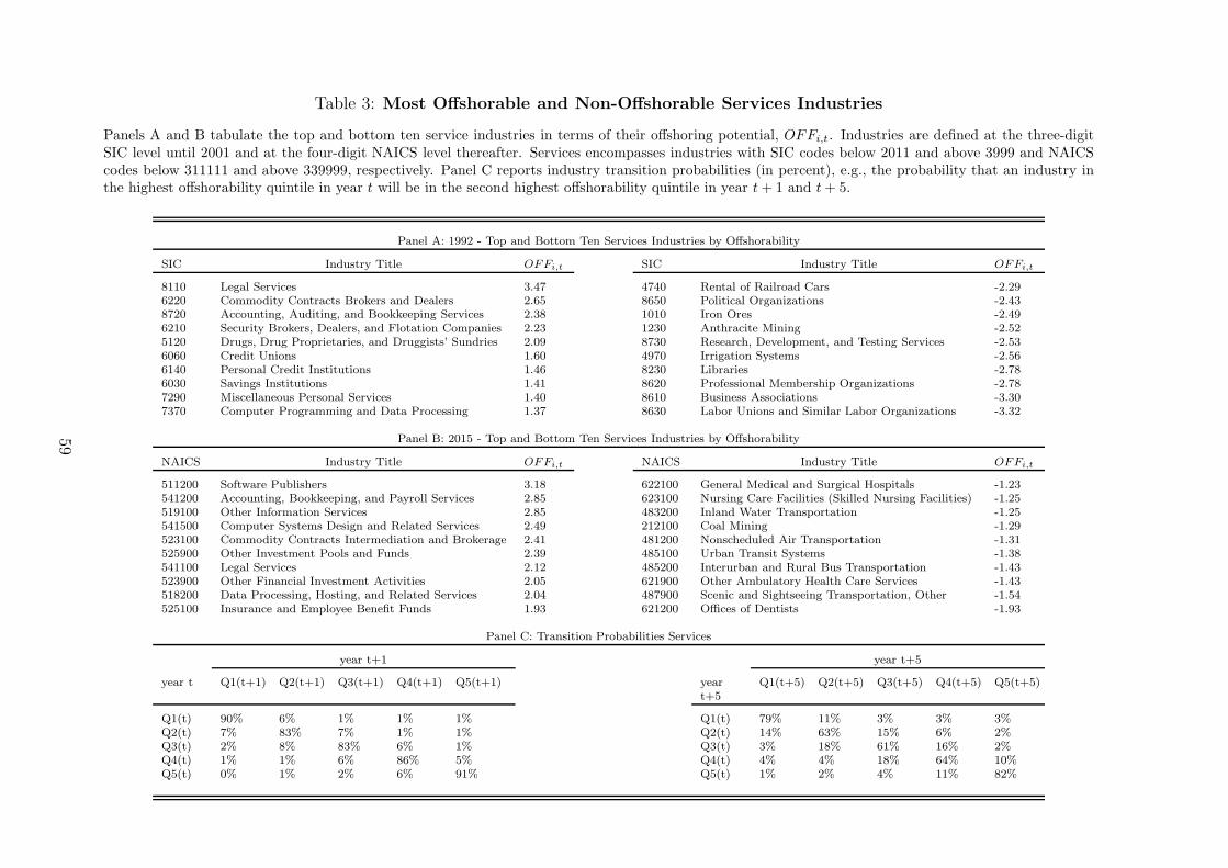
Table 3: Most Offshorable and Non-Offshorable Services Industries

Panels A and B tabulate the top and bottom ten service industries in terms of their offshoring potential, OFFi,t. Industries are defined at the three-digitSIC level until 2001 and at the four-digit NAICS level thereafter. Services encompasses industries with SIC codes below 2011 and above 3999 and NAICScodes below 311111 and above 339999, respectively. Panel C reports industry transition probabilities (in percent), e.g., the probability that an industry inthe highest offshorability quintile in year t will be in the second highest offshorability quintile in year t+ 1 and t+ 5.

Panel A: 1992 - Top and Bottom Ten Services Industries by Offshorability

SIC Industry Title OFFi,t SIC Industry Title OFFi,t

8110 Legal Services 3.47 4740 Rental of Railroad Cars -2.296220 Commodity Contracts Brokers and Dealers 2.65 8650 Political Organizations -2.438720 Accounting, Auditing, and Bookkeeping Services 2.38 1010 Iron Ores -2.496210 Security Brokers, Dealers, and Flotation Companies 2.23 1230 Anthracite Mining -2.525120 Drugs, Drug Proprietaries, and Druggists’ Sundries 2.09 8730 Research, Development, and Testing Services -2.536060 Credit Unions 1.60 4970 Irrigation Systems -2.566140 Personal Credit Institutions 1.46 8230 Libraries -2.786030 Savings Institutions 1.41 8620 Professional Membership Organizations -2.787290 Miscellaneous Personal Services 1.40 8610 Business Associations -3.307370 Computer Programming and Data Processing 1.37 8630 Labor Unions and Similar Labor Organizations -3.32

Panel B: 2015 - Top and Bottom Ten Services Industries by Offshorability

NAICS Industry Title OFFi,t NAICS Industry Title OFFi,t

511200 Software Publishers 3.18 622100 General Medical and Surgical Hospitals -1.23541200 Accounting, Bookkeeping, and Payroll Services 2.85 623100 Nursing Care Facilities (Skilled Nursing Facilities) -1.25519100 Other Information Services 2.85 483200 Inland Water Transportation -1.25541500 Computer Systems Design and Related Services 2.49 212100 Coal Mining -1.29523100 Commodity Contracts Intermediation and Brokerage 2.41 481200 Nonscheduled Air Transportation -1.31525900 Other Investment Pools and Funds 2.39 485100 Urban Transit Systems -1.38541100 Legal Services 2.12 485200 Interurban and Rural Bus Transportation -1.43523900 Other Financial Investment Activities 2.05 621900 Other Ambulatory Health Care Services -1.43518200 Data Processing, Hosting, and Related Services 2.04 487900 Scenic and Sightseeing Transportation, Other -1.54525100 Insurance and Employee Benefit Funds 1.93 621200 Offices of Dentists -1.93

Panel C: Transition Probabilities Services

year t+1 year t+5

year t Q1(t+1) Q2(t+1) Q3(t+1) Q4(t+1) Q5(t+1) yeart+5

Q1(t+5) Q2(t+5) Q3(t+5) Q4(t+5) Q5(t+5)

Q1(t) 90% 6% 1% 1% 1% Q1(t) 79% 11% 3% 3% 3%Q2(t) 7% 83% 7% 1% 1% Q2(t) 14% 63% 15% 6% 2%Q3(t) 2% 8% 83% 6% 1% Q3(t) 3% 18% 61% 16% 2%Q4(t) 1% 1% 6% 86% 5% Q4(t) 4% 4% 18% 64% 10%Q5(t) 0% 1% 2% 6% 91% Q5(t) 1% 2% 4% 11% 82%

59

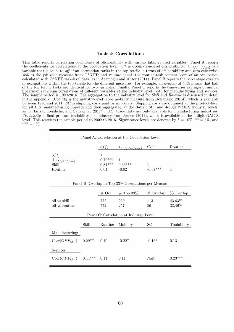
Table 4: Correlations

This table reports correlation coefficients of offshorability with various labor-related variables. Panel A reportsthe coefficients for correlations at the occupation level. off is occupation-level offshorability; 1offj>offp66 is avariable that is equal to off if an occupation ranks in the top tercile in terms of offshorability and zero otherwise;skill is the job zone measure from O*NET; and routine equals the routine-task content score of an occupationcalculated with O*NET task-level data, as in Acemoglu and Autor (2011). Panel B reports the percentage overlapin occupations within the top tercile for the different measures. For example, an overlap of 50% means that halfof the top tercile tasks are identical for two variables. Finally, Panel C reports the time-series averages of annualSpearman rank sum correlations of different variables at the industry level, both for manufacturing and services.The sample period is 1990-2016. The aggregation to the industry level for Skill and Routine is discussed in detailin the appendix. Mobility is the industry-level labor mobility measure from Donangelo (2014), which is availablebetween 1990 and 2011. SC is shipping costs paid by importers. Shipping costs are obtained at the product-levelfor all U.S. manufacturing imports and then aggregated at the 3-digit SIC and 4-digit NAICS industry levels,as in Barrot, Loualiche, and Sauvagnat (2017). U.S. trade data are only available for manufacturing industries.Tradability is final product tradability per industry from Jensen (2011), which is available at the 4-digit NAICSlevel. This restricts the sample period to 2002 to 2016. Significance levels are denoted by * = 10%, ** = 5%, and*** = 1%.

Panel A: Correlation at the Occupation Level

offj 1offj>offp66 Skill Routine

offj 11offj>offp66 0.79*** 1Skill 0.31*** 0.33*** 1Routine 0.04 -0.02 -0.67*** 1

Panel B: Overlap in Top 33% Occupations per Measure

# Occ # Top 33% # Overlap %-Overlap

off vs skill 772 259 113 43.63%off vs routine 772 257 86 33.46%

Panel C: Correlation at Industry Level

Skill Routine Mobility SC Tradability

Manufacturing:

Corr(OFFi,t, ) 0.29** 0.10 -0.22* -0.16* 0.13

Services:

Corr(OFFi,t, ) 0.44*** 0.14 0.11 NaN 0.23***

60

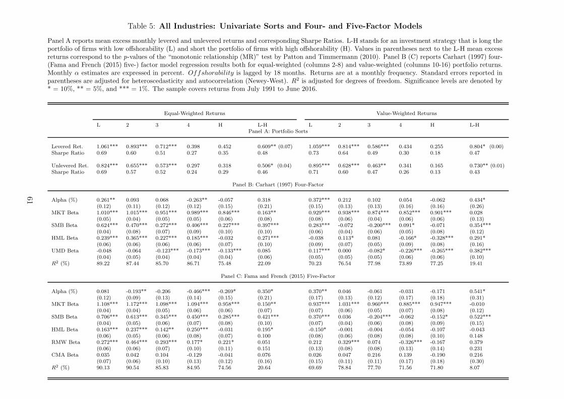
Table 5: All Industries: Univariate Sorts and Four- and Five-Factor Models

Panel A reports mean excess monthly levered and unlevered returns and corresponding Sharpe Ratios. L-H stands for an investment strategy that is long theportfolio of firms with low offshorability (L) and short the portfolio of firms with high offshorability (H). Values in parentheses next to the L-H mean excessreturns correspond to the p-values of the “monotonic relationship (MR)” test by Patton and Timmermann (2010). Panel B (C) reports Carhart (1997) four-(Fama and French (2015) five-) factor model regression results both for equal-weighted (columns 2-8) and value-weighted (columns 10-16) portfolio returns.Monthly α estimates are expressed in percent. Offshorability is lagged by 18 months. Returns are at a monthly frequency. Standard errors reported inparentheses are adjusted for heteroscedasticity and autocorrelation (Newey-West). R2 is adjusted for degrees of freedom. Significance levels are denoted by* = 10%, ** = 5%, and *** = 1%. The sample covers returns from July 1991 to June 2016.

Equal-Weighted Returns Value-Weighted Returns

L 2 3 4 H L-H L 2 3 4 H L-HPanel A: Portfolio Sorts

Levered Ret. 1.061*** 0.893*** 0.712*** 0.398 0.452 0.609** (0.07) 1.059*** 0.814*** 0.586*** 0.434 0.255 0.804* (0.00)Sharpe Ratio 0.69 0.60 0.51 0.27 0.35 0.48 0.73 0.64 0.49 0.30 0.18 0.47

Unlevered Ret. 0.824*** 0.655*** 0.573*** 0.297 0.318 0.506* (0.04) 0.895*** 0.628*** 0.463** 0.341 0.165 0.730** (0.01)Sharpe Ratio 0.69 0.57 0.52 0.24 0.29 0.46 0.71 0.60 0.47 0.26 0.13 0.43

Panel B: Carhart (1997) Four-Factor

Alpha (%) 0.261** 0.093 0.068 -0.263** -0.057 0.318 0.372*** 0.212 0.102 0.054 -0.062 0.434*(0.12) (0.11) (0.12) (0.12) (0.15) (0.21) (0.15) (0.13) (0.13) (0.16) (0.16) (0.26)

MKT Beta 1.010*** 1.015*** 0.951*** 0.989*** 0.846*** 0.163** 0.929*** 0.938*** 0.874*** 0.852*** 0.901*** 0.028(0.05) (0.04) (0.05) (0.05) (0.06) (0.08) (0.08) (0.06) (0.04) (0.06) (0.06) (0.13)

SMB Beta 0.624*** 0.470*** 0.272*** 0.406*** 0.227*** 0.397*** 0.283*** -0.072 -0.200*** 0.091* -0.071 0.354***(0.04) (0.08) (0.07) (0.09) (0.10) (0.10) (0.06) (0.04) (0.06) (0.05) (0.08) (0.12)

HML Beta 0.239*** 0.365*** 0.227*** 0.185*** -0.032 0.271*** -0.038 0.113* 0.081 -0.166* -0.328*** 0.291*(0.06) (0.06) (0.06) (0.06) (0.07) (0.10) (0.09) (0.07) (0.05) (0.09) (0.08) (0.16)

UMD Beta -0.048 -0.064 -0.123*** -0.173*** -0.133*** 0.085 0.117*** 0.000 -0.082* -0.226*** -0.265*** 0.382***(0.04) (0.05) (0.04) (0.04) (0.04) (0.06) (0.05) (0.05) (0.05) (0.06) (0.06) (0.10)

R2 (%) 89.22 87.44 85.70 86.71 75.48 22.09 70.23 76.54 77.98 73.89 77.25 19.41

Panel C: Fama and French (2015) Five-Factor

Alpha (%) 0.081 -0.193** -0.206 -0.466*** -0.269* 0.350* 0.370** 0.046 -0.061 -0.031 -0.171 0.541*(0.12) (0.09) (0.13) (0.14) (0.15) (0.21) (0.17) (0.13) (0.12) (0.17) (0.18) (0.31)

MKT Beta 1.108*** 1.172*** 1.098*** 1.094*** 0.958*** 0.150** 0.937*** 1.031*** 0.960*** 0.885*** 0.947*** -0.010(0.04) (0.04) (0.05) (0.06) (0.06) (0.07) (0.07) (0.06) (0.05) (0.07) (0.08) (0.12)

SMB Beta 0.706*** 0.613*** 0.345*** 0.450*** 0.285*** 0.421*** 0.370*** 0.036 -0.204*** -0.062 -0.152* 0.522***(0.04) (0.05) (0.06) (0.07) (0.08) (0.10) (0.07) (0.04) (0.06) (0.08) (0.09) (0.15)

HML Beta 0.163*** 0.237*** 0.142** 0.250*** -0.031 0.195* -0.150* -0.001 -0.004 -0.054 -0.107 -0.043(0.06) (0.05) (0.06) (0.08) (0.07) 0.100 (0.08) (0.06) (0.08) (0.08) (0.10) 0.148

RMW Beta 0.272*** 0.464*** 0.293*** 0.177* 0.221* 0.051 0.212 0.329*** 0.074 -0.326*** -0.167 0.379(0.06) (0.06) (0.07) (0.10) (0.11) 0.151 (0.13) (0.08) (0.08) (0.13) (0.14) 0.231

CMA Beta 0.035 0.042 0.104 -0.129 -0.041 0.076 0.026 0.047 0.216 0.139 -0.190 0.216(0.07) (0.06) (0.10) (0.13) (0.12) (0.16) (0.15) (0.11) (0.11) (0.17) (0.18) (0.30)

R2 (%) 90.13 90.54 85.83 84.95 74.56 20.64 69.69 78.84 77.70 71.56 71.80 8.07

61

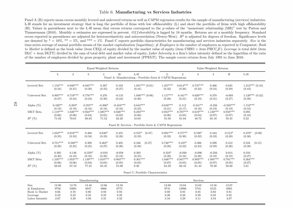
Table 6: Manufacturing vs Services Industries

Panel A (B) reports mean excess monthly levered and unlevered returns as well as CAPM regression results for the sample of manufacturing (services) industries.L-H stands for an investment strategy that is long the portfolio of firms with low offshorability (L) and short the portfolio of firms with high offshorability(H). Values in parentheses next to the L-H mean that excess returns correspond to the p-values of the “monotonic relationship (MR)” test by Patton andTimmermann (2010). Monthly α estimates are expressed in percent. Offshorability is lagged by 18 months. Returns are at a monthly frequency. Standarderrors reported in parentheses are adjusted for heteroscedasticity and autocorrelation (Newey-West). R2 is adjusted for degrees of freedom. Significance levelsare denoted by * = 10%, ** = 5%, and *** = 1%. Panel C reports portfolio characteristics for manufacturing and services industries separately. Size is thetime-series average of annual portfolio means of the market capitalization (logarithm); # Employees is the number of employees as reported in Compustat; Bookto Market is defined as the book value (item CEQ) of equity divided by the market value of equity (item CSHO × item PRCC F); Leverage is total debt (itemDLC + item DLTT) divided by the sum of total debt and market value of equity; Labor Intensity is a firm’s labor intensity defined as the logarithm of the ratioof the number of employees divided by gross property, plant and investment (PPEGT). The sample covers returns from July 1991 to June 2016.

Equal-Weighted Returns Value-Weighted Returns

L 2 3 4 H L-H L 2 3 4 H L-HPanel A: Manufacturing - Portfolio Sorts & CAPM Regressions

Levered Ret. 1.134*** 0.949*** 0.945*** 0.387 0.103 1.031*** (0.01) 1.257*** 0.614*** 0.737*** 0.466 0.045 1.212*** (0.16)(0.34) (0.31) (0.29) (0.33) (0.27) (0.44) (0.32) (0.26) (0.22) (0.34) (0.29) (0.43)

Unlevered Ret. 0.905*** 0.719*** 0.776*** 0.276 -0.131 1.036*** (0.06) 1.117*** 0.441** 0.620*** 0.378 -0.003 1.120*** (0.22)(0.27) (0.24) (0.24) (0.30) (0.24) (0.36) (0.28) (0.21) (0.19) (0.31) (0.27) (0.39)

Alpha (%) 0.420** 0.293* 0.355** -0.306* -0.424*** 0.844*** 0.649*** 0.112 0.341** -0.256 -0.503*** 1.152***(0.19) (0.18) (0.16) (0.18) (0.16) (0.23) (0.21) (0.17) (0.16) (0.19) (0.19) (0.34)

MKT Beta 1.119*** 1.026*** 0.924*** 1.085*** 0.826*** 0.293*** 0.953*** 0.787*** 0.619*** 1.130*** 0.858*** 0.095(0.06) (0.06) (0.04) (0.05) (0.03) (0.06) (0.06) (0.05) (0.04) (0.07) (0.07) (0.10)

R2 (%) 71.02 70.61 68.83 71.52 62.20 10.03 55.50 61.84 48.72 65.16 59.45 0.22

Panel B: Services - Portfolio Sorts & CAPM Regressions

Levered Ret. 1.010*** 0.818*** 0.468 0.640* 0.455 0.555* (0.27) 0.991*** 0.577** 0.538* 0.444 0.513* 0.478* (0.06)(0.35) (0.33) (0.34) (0.33) (0.28) (0.33) (0.33) (0.30) (0.32) (0.33) (0.28) (0.30)

Unlevered Ret. 0.751*** 0.568** 0.309 0.462* 0.405 0.346 (0.37) 0.746*** 0.437* 0.366 0.298 0.412 0.334 (0.15)(0.28) (0.25) (0.25) (0.27) (0.26) (0.38) (0.28) (0.23) (0.24) (0.29) (0.26) (0.38)

Alpha (%) 0.305 0.146 -0.259* -0.010 -0.058 0.363 0.324* -0.028 -0.096 -0.256 0.014 0.310(0.20) (0.19) (0.16) (0.20) (0.19) (0.25) (0.20) (0.16) (0.20) (0.18) (0.19) (0.27)

MKT Beta 1.105*** 1.053*** 1.139*** 1.018*** 0.803*** 0.301*** 1.046*** 0.947*** 0.993*** 1.095*** 0.781*** 0.264***(0.06) (0.06) (0.04) (0.05) (0.05) (0.05) (0.07) (0.05) (0.05) (0.07) (0.05) (0.07)

R2 (%) 68.65 67.53 77.55 65.35 55.98 9.30 64.39 66.42 61.44 70.30 50.80 5.61

Panel C: Portfolio Characteristics

Manufacturing Services

Size 12.80 12.70 12.48 12.66 12.58 12.69 13.04 12.63 12.56 12.67# Employees 9756 10091 6947 6866 6775 9741 12996 5745 6125 9365Book to Market 0.66 0.76 0.86 0.92 0.93 0.80 0.85 0.85 0.82 0.81Leverage 0.23 0.23 0.24 0.25 0.28 0.26 0.28 0.29 0.23 0.25Labor Intensity 2.67 3.20 3.56 3.31 3.32 3.18 3.29 3.11 3.54 4.07

62

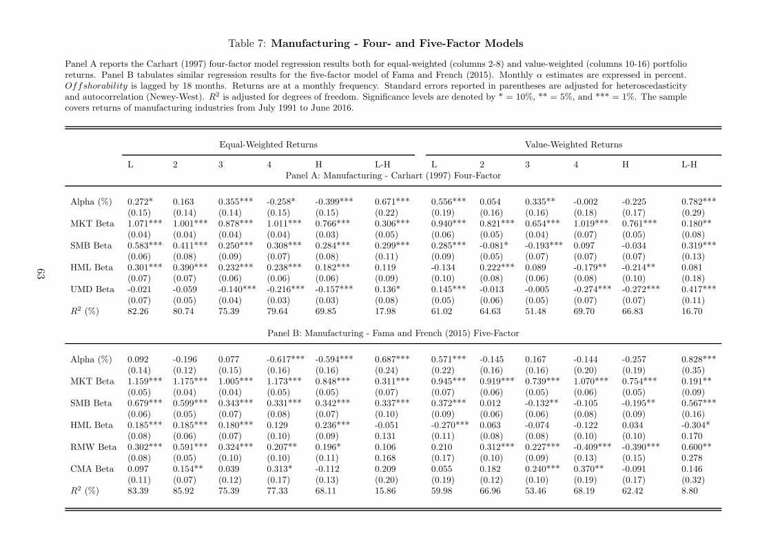
Table 7: Manufacturing - Four- and Five-Factor Models

Panel A reports the Carhart (1997) four-factor model regression results both for equal-weighted (columns 2-8) and value-weighted (columns 10-16) portfolioreturns. Panel B tabulates similar regression results for the five-factor model of Fama and French (2015). Monthly α estimates are expressed in percent.Offshorability is lagged by 18 months. Returns are at a monthly frequency. Standard errors reported in parentheses are adjusted for heteroscedasticityand autocorrelation (Newey-West). R2 is adjusted for degrees of freedom. Significance levels are denoted by * = 10%, ** = 5%, and *** = 1%. The samplecovers returns of manufacturing industries from July 1991 to June 2016.

Equal-Weighted Returns Value-Weighted Returns

L 2 3 4 H L-H L 2 3 4 H L-HPanel A: Manufacturing - Carhart (1997) Four-Factor

Alpha (%) 0.272* 0.163 0.355*** -0.258* -0.399*** 0.671*** 0.556*** 0.054 0.335** -0.002 -0.225 0.782***(0.15) (0.14) (0.14) (0.15) (0.15) (0.22) (0.19) (0.16) (0.16) (0.18) (0.17) (0.29)

MKT Beta 1.071*** 1.001*** 0.878*** 1.011*** 0.766*** 0.306*** 0.940*** 0.821*** 0.654*** 1.019*** 0.761*** 0.180**(0.04) (0.04) (0.04) (0.04) (0.03) (0.05) (0.06) (0.05) (0.04) (0.07) (0.05) (0.08)

SMB Beta 0.583*** 0.411*** 0.250*** 0.308*** 0.284*** 0.299*** 0.285*** -0.081* -0.193*** 0.097 -0.034 0.319***(0.06) (0.08) (0.09) (0.07) (0.08) (0.11) (0.09) (0.05) (0.07) (0.07) (0.07) (0.13)

HML Beta 0.301*** 0.390*** 0.232*** 0.238*** 0.182*** 0.119 -0.134 0.222*** 0.089 -0.179** -0.214** 0.081(0.07) (0.07) (0.06) (0.06) (0.06) (0.09) (0.10) (0.08) (0.06) (0.08) (0.10) (0.18)

UMD Beta -0.021 -0.059 -0.140*** -0.216*** -0.157*** 0.136* 0.145*** -0.013 -0.005 -0.274*** -0.272*** 0.417***(0.07) (0.05) (0.04) (0.03) (0.03) (0.08) (0.05) (0.06) (0.05) (0.07) (0.07) (0.11)

R2 (%) 82.26 80.74 75.39 79.64 69.85 17.98 61.02 64.63 51.48 69.70 66.83 16.70

Panel B: Manufacturing - Fama and French (2015) Five-Factor

Alpha (%) 0.092 -0.196 0.077 -0.617*** -0.594*** 0.687*** 0.571*** -0.145 0.167 -0.144 -0.257 0.828***(0.14) (0.12) (0.15) (0.16) (0.16) (0.24) (0.22) (0.16) (0.16) (0.20) (0.19) (0.35)

MKT Beta 1.159*** 1.175*** 1.005*** 1.173*** 0.848*** 0.311*** 0.945*** 0.919*** 0.739*** 1.070*** 0.754*** 0.191**(0.05) (0.04) (0.04) (0.05) (0.05) (0.07) (0.07) (0.06) (0.05) (0.06) (0.05) (0.09)

SMB Beta 0.679*** 0.599*** 0.343*** 0.331*** 0.342*** 0.337*** 0.372*** 0.012 -0.132** -0.105 -0.195** 0.567***(0.06) (0.05) (0.07) (0.08) (0.07) (0.10) (0.09) (0.06) (0.06) (0.08) (0.09) (0.16)

HML Beta 0.185*** 0.185*** 0.180*** 0.129 0.236*** -0.051 -0.270*** 0.063 -0.074 -0.122 0.034 -0.304*(0.08) (0.06) (0.07) (0.10) (0.09) 0.131 (0.11) (0.08) (0.08) (0.10) (0.10) 0.170

RMW Beta 0.302*** 0.591*** 0.324*** 0.207** 0.196* 0.106 0.210 0.312*** 0.227*** -0.409*** -0.390*** 0.600**(0.08) (0.05) (0.10) (0.10) (0.11) 0.168 (0.17) (0.10) (0.09) (0.13) (0.15) 0.278

CMA Beta 0.097 0.154** 0.039 0.313* -0.112 0.209 0.055 0.182 0.240*** 0.370** -0.091 0.146(0.11) (0.07) (0.12) (0.17) (0.13) (0.20) (0.19) (0.12) (0.10) (0.19) (0.17) (0.32)

R2 (%) 83.39 85.92 75.39 77.33 68.11 15.86 59.98 66.96 53.46 68.19 62.42 8.80

63

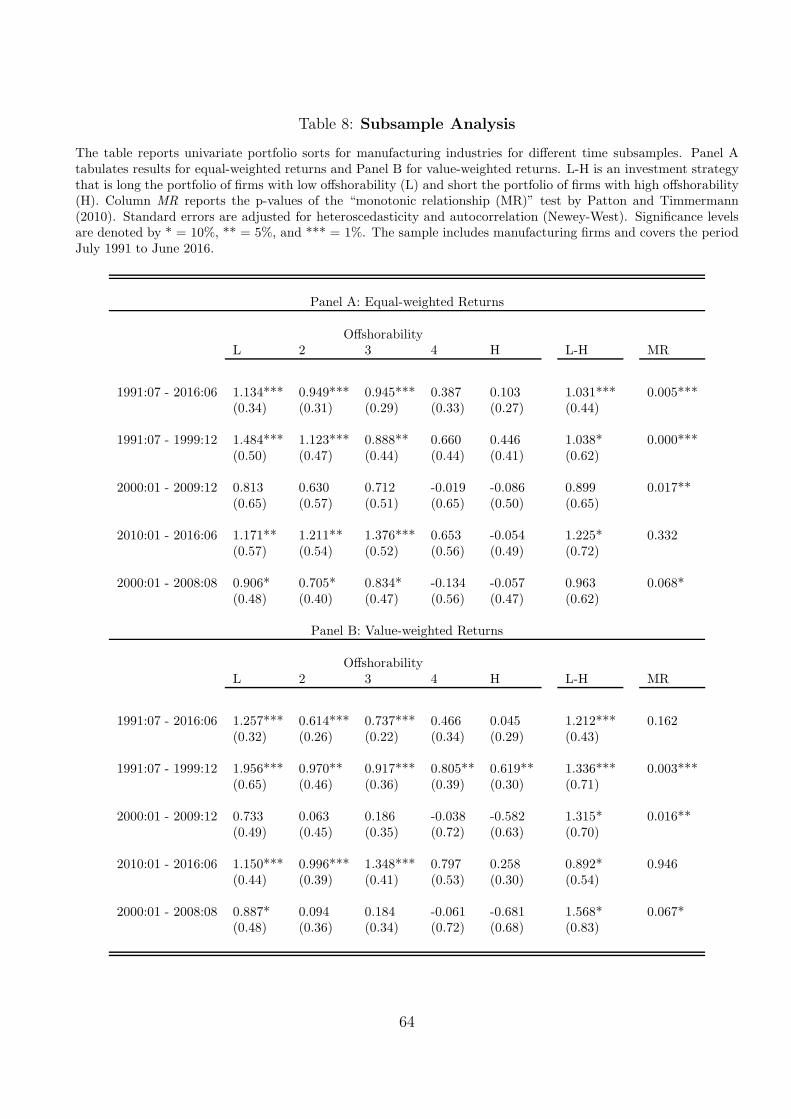
Table 8: Subsample Analysis

The table reports univariate portfolio sorts for manufacturing industries for different time subsamples. Panel Atabulates results for equal-weighted returns and Panel B for value-weighted returns. L-H is an investment strategythat is long the portfolio of firms with low offshorability (L) and short the portfolio of firms with high offshorability(H). Column MR reports the p-values of the “monotonic relationship (MR)” test by Patton and Timmermann(2010). Standard errors are adjusted for heteroscedasticity and autocorrelation (Newey-West). Significance levelsare denoted by * = 10%, ** = 5%, and *** = 1%. The sample includes manufacturing firms and covers the periodJuly 1991 to June 2016.

Panel A: Equal-weighted Returns

OffshorabilityL 2 3 4 H L-H MR

1991:07 - 2016:06 1.134*** 0.949*** 0.945*** 0.387 0.103 1.031*** 0.005***(0.34) (0.31) (0.29) (0.33) (0.27) (0.44)

1991:07 - 1999:12 1.484*** 1.123*** 0.888** 0.660 0.446 1.038* 0.000***(0.50) (0.47) (0.44) (0.44) (0.41) (0.62)

2000:01 - 2009:12 0.813 0.630 0.712 -0.019 -0.086 0.899 0.017**(0.65) (0.57) (0.51) (0.65) (0.50) (0.65)

2010:01 - 2016:06 1.171** 1.211** 1.376*** 0.653 -0.054 1.225* 0.332(0.57) (0.54) (0.52) (0.56) (0.49) (0.72)

2000:01 - 2008:08 0.906* 0.705* 0.834* -0.134 -0.057 0.963 0.068*(0.48) (0.40) (0.47) (0.56) (0.47) (0.62)

Panel B: Value-weighted Returns

OffshorabilityL 2 3 4 H L-H MR

1991:07 - 2016:06 1.257*** 0.614*** 0.737*** 0.466 0.045 1.212*** 0.162(0.32) (0.26) (0.22) (0.34) (0.29) (0.43)

1991:07 - 1999:12 1.956*** 0.970** 0.917*** 0.805** 0.619** 1.336*** 0.003***(0.65) (0.46) (0.36) (0.39) (0.30) (0.71)

2000:01 - 2009:12 0.733 0.063 0.186 -0.038 -0.582 1.315* 0.016**(0.49) (0.45) (0.35) (0.72) (0.63) (0.70)

2010:01 - 2016:06 1.150*** 0.996*** 1.348*** 0.797 0.258 0.892* 0.946(0.44) (0.39) (0.41) (0.53) (0.30) (0.54)

2000:01 - 2008:08 0.887* 0.094 0.184 -0.061 -0.681 1.568* 0.067*(0.48) (0.36) (0.34) (0.72) (0.68) (0.83)

64

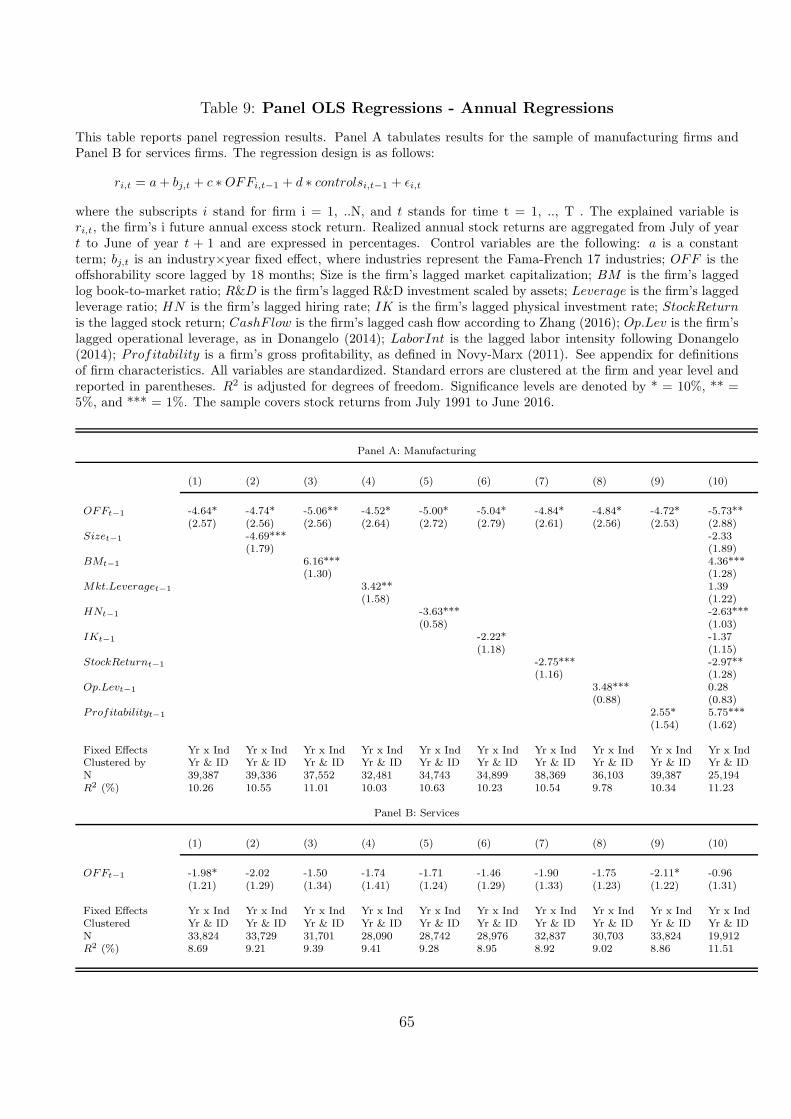
Table 9: Panel OLS Regressions - Annual Regressions

This table reports panel regression results. Panel A tabulates results for the sample of manufacturing firms andPanel B for services firms. The regression design is as follows:

ri,t = a+ bj,t + c ∗OFFi,t−1 + d ∗ controlsi,t−1 + ǫi,t

where the subscripts i stand for firm i = 1, ..N, and t stands for time t = 1, .., T . The explained variable isri,t, the firm’s i future annual excess stock return. Realized annual stock returns are aggregated from July of yeart to June of year t + 1 and are expressed in percentages. Control variables are the following: a is a constantterm; bj,t is an industry×year fixed effect, where industries represent the Fama-French 17 industries; OFF is theoffshorability score lagged by 18 months; Size is the firm’s lagged market capitalization; BM is the firm’s laggedlog book-to-market ratio; R&D is the firm’s lagged R&D investment scaled by assets; Leverage is the firm’s laggedleverage ratio; HN is the firm’s lagged hiring rate; IK is the firm’s lagged physical investment rate; StockReturnis the lagged stock return; CashF low is the firm’s lagged cash flow according to Zhang (2016); Op.Lev is the firm’slagged operational leverage, as in Donangelo (2014); LaborInt is the lagged labor intensity following Donangelo(2014); Profitability is a firm’s gross profitability, as defined in Novy-Marx (2011). See appendix for definitionsof firm characteristics. All variables are standardized. Standard errors are clustered at the firm and year level andreported in parentheses. R2 is adjusted for degrees of freedom. Significance levels are denoted by * = 10%, ** =5%, and *** = 1%. The sample covers stock returns from July 1991 to June 2016.

Panel A: Manufacturing

(1) (2) (3) (4) (5) (6) (7) (8) (9) (10)

OFFt−1 -4.64* -4.74* -5.06** -4.52* -5.00* -5.04* -4.84* -4.84* -4.72* -5.73**(2.57) (2.56) (2.56) (2.64) (2.72) (2.79) (2.61) (2.56) (2.53) (2.88)

Sizet−1 -4.69*** -2.33(1.79) (1.89)

BMt−1 6.16*** 4.36***(1.30) (1.28)

Mkt.Leveraget−1 3.42** 1.39(1.58) (1.22)

HNt−1 -3.63*** -2.63***(0.58) (1.03)

IKt−1 -2.22* -1.37(1.18) (1.15)

StockReturnt−1 -2.75*** -2.97**(1.16) (1.28)

Op.Levt−1 3.48*** 0.28(0.88) (0.83)

Profitabilityt−1 2.55* 5.75***(1.54) (1.62)

Fixed Effects Yr x Ind Yr x Ind Yr x Ind Yr x Ind Yr x Ind Yr x Ind Yr x Ind Yr x Ind Yr x Ind Yr x IndClustered by Yr & ID Yr & ID Yr & ID Yr & ID Yr & ID Yr & ID Yr & ID Yr & ID Yr & ID Yr & IDN 39,387 39,336 37,552 32,481 34,743 34,899 38,369 36,103 39,387 25,194R2 (%) 10.26 10.55 11.01 10.03 10.63 10.23 10.54 9.78 10.34 11.23

Panel B: Services

(1) (2) (3) (4) (5) (6) (7) (8) (9) (10)

OFFt−1 -1.98* -2.02 -1.50 -1.74 -1.71 -1.46 -1.90 -1.75 -2.11* -0.96(1.21) (1.29) (1.34) (1.41) (1.24) (1.29) (1.33) (1.23) (1.22) (1.31)

Fixed Effects Yr x Ind Yr x Ind Yr x Ind Yr x Ind Yr x Ind Yr x Ind Yr x Ind Yr x Ind Yr x Ind Yr x IndClustered Yr & ID Yr & ID Yr & ID Yr & ID Yr & ID Yr & ID Yr & ID Yr & ID Yr & ID Yr & IDN 33,824 33,729 31,701 28,090 28,742 28,976 32,837 30,703 33,824 19,912R2 (%) 8.69 9.21 9.39 9.41 9.28 8.95 8.92 9.02 8.86 11.51

65

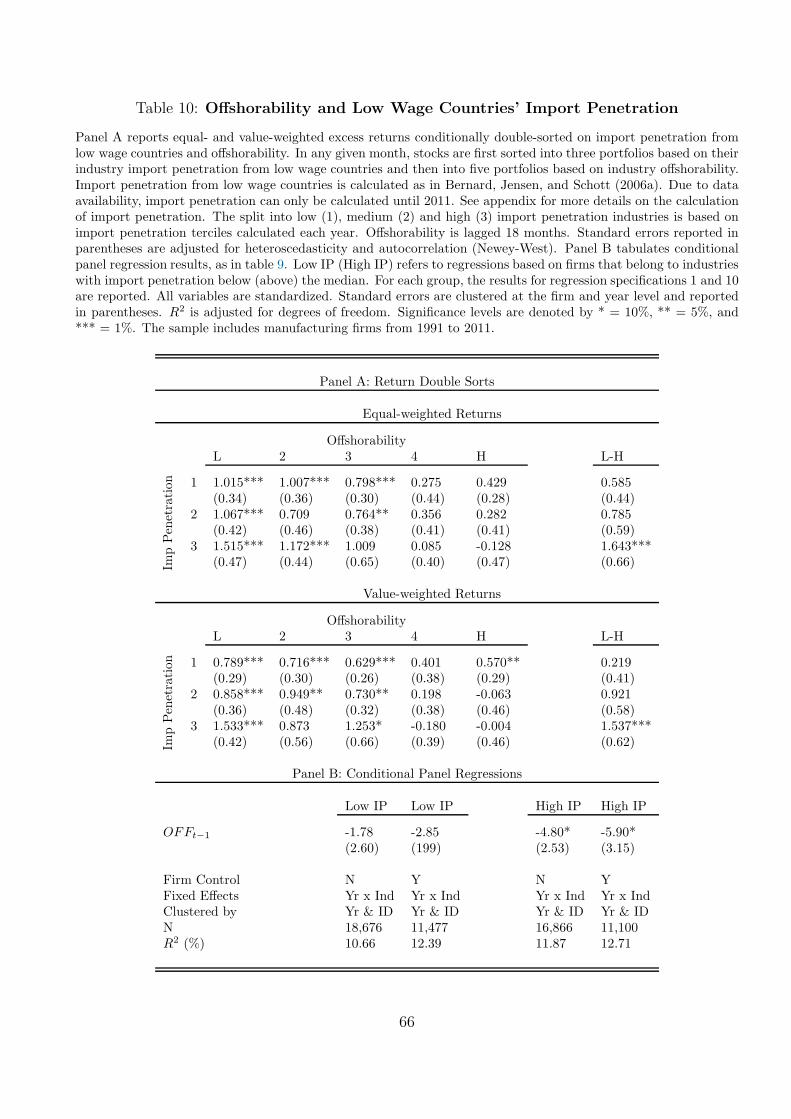
Table 10: Offshorability and Low Wage Countries’ Import Penetration

Panel A reports equal- and value-weighted excess returns conditionally double-sorted on import penetration fromlow wage countries and offshorability. In any given month, stocks are first sorted into three portfolios based on theirindustry import penetration from low wage countries and then into five portfolios based on industry offshorability.Import penetration from low wage countries is calculated as in Bernard, Jensen, and Schott (2006a). Due to dataavailability, import penetration can only be calculated until 2011. See appendix for more details on the calculationof import penetration. The split into low (1), medium (2) and high (3) import penetration industries is based onimport penetration terciles calculated each year. Offshorability is lagged 18 months. Standard errors reported inparentheses are adjusted for heteroscedasticity and autocorrelation (Newey-West). Panel B tabulates conditionalpanel regression results, as in table 9. Low IP (High IP) refers to regressions based on firms that belong to industrieswith import penetration below (above) the median. For each group, the results for regression specifications 1 and 10are reported. All variables are standardized. Standard errors are clustered at the firm and year level and reportedin parentheses. R2 is adjusted for degrees of freedom. Significance levels are denoted by * = 10%, ** = 5%, and*** = 1%. The sample includes manufacturing firms from 1991 to 2011.

Panel A: Return Double Sorts

Equal-weighted Returns

OffshorabilityL 2 3 4 H L-H

ImpPenetration 1 1.015*** 1.007*** 0.798*** 0.275 0.429 0.585

(0.34) (0.36) (0.30) (0.44) (0.28) (0.44)2 1.067*** 0.709 0.764** 0.356 0.282 0.785

(0.42) (0.46) (0.38) (0.41) (0.41) (0.59)3 1.515*** 1.172*** 1.009 0.085 -0.128 1.643***

(0.47) (0.44) (0.65) (0.40) (0.47) (0.66)

Value-weighted Returns

OffshorabilityL 2 3 4 H L-H

ImpPenetration 1 0.789*** 0.716*** 0.629*** 0.401 0.570** 0.219

(0.29) (0.30) (0.26) (0.38) (0.29) (0.41)2 0.858*** 0.949** 0.730** 0.198 -0.063 0.921

(0.36) (0.48) (0.32) (0.38) (0.46) (0.58)3 1.533*** 0.873 1.253* -0.180 -0.004 1.537***

(0.42) (0.56) (0.66) (0.39) (0.46) (0.62)

Panel B: Conditional Panel Regressions

Low IP Low IP High IP High IP

OFFt−1 -1.78 -2.85 -4.80* -5.90*(2.60) (199) (2.53) (3.15)

Firm Control N Y N YFixed Effects Yr x Ind Yr x Ind Yr x Ind Yr x IndClustered by Yr & ID Yr & ID Yr & ID Yr & IDN 18,676 11,477 16,866 11,100R2 (%) 10.66 12.39 11.87 12.71

66

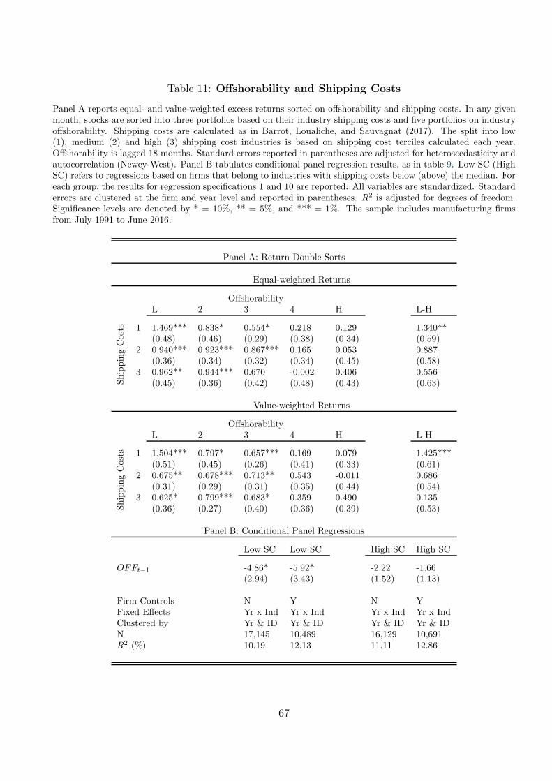
Table 11: Offshorability and Shipping Costs

Panel A reports equal- and value-weighted excess returns sorted on offshorability and shipping costs. In any givenmonth, stocks are sorted into three portfolios based on their industry shipping costs and five portfolios on industryoffshorability. Shipping costs are calculated as in Barrot, Loualiche, and Sauvagnat (2017). The split into low(1), medium (2) and high (3) shipping cost industries is based on shipping cost terciles calculated each year.Offshorability is lagged 18 months. Standard errors reported in parentheses are adjusted for heteroscedasticity andautocorrelation (Newey-West). Panel B tabulates conditional panel regression results, as in table 9. Low SC (HighSC) refers to regressions based on firms that belong to industries with shipping costs below (above) the median. Foreach group, the results for regression specifications 1 and 10 are reported. All variables are standardized. Standarderrors are clustered at the firm and year level and reported in parentheses. R2 is adjusted for degrees of freedom.Significance levels are denoted by * = 10%, ** = 5%, and *** = 1%. The sample includes manufacturing firmsfrom July 1991 to June 2016.

Panel A: Return Double Sorts

Equal-weighted Returns

OffshorabilityL 2 3 4 H L-H

ShippingCosts 1 1.469*** 0.838* 0.554* 0.218 0.129 1.340**

(0.48) (0.46) (0.29) (0.38) (0.34) (0.59)2 0.940*** 0.923*** 0.867*** 0.165 0.053 0.887

(0.36) (0.34) (0.32) (0.34) (0.45) (0.58)3 0.962** 0.944*** 0.670 -0.002 0.406 0.556

(0.45) (0.36) (0.42) (0.48) (0.43) (0.63)

Value-weighted Returns

OffshorabilityL 2 3 4 H L-H

ShippingCosts 1 1.504*** 0.797* 0.657*** 0.169 0.079 1.425***

(0.51) (0.45) (0.26) (0.41) (0.33) (0.61)2 0.675** 0.678*** 0.713** 0.543 -0.011 0.686

(0.31) (0.29) (0.31) (0.35) (0.44) (0.54)3 0.625* 0.799*** 0.683* 0.359 0.490 0.135

(0.36) (0.27) (0.40) (0.36) (0.39) (0.53)

Panel B: Conditional Panel Regressions

Low SC Low SC High SC High SC

OFFt−1 -4.86* -5.92* -2.22 -1.66(2.94) (3.43) (1.52) (1.13)

Firm Controls N Y N YFixed Effects Yr x Ind Yr x Ind Yr x Ind Yr x IndClustered by Yr & ID Yr & ID Yr & ID Yr & IDN 17,145 10,489 16,129 10,691R2 (%) 10.19 12.13 11.11 12.86

67

Table 12: Offshorability and Multinational Companies

Panel A reports the post-ranking mean of equal- and value-weighted excess returns of stocks sorted on offshorabilityfor multinational manufacturing firms and domestic manufacturing firms. Excess Returns are calculated as realizedmonthly returns minus the one-month risk-free rate. EW refers to equal-weighted and VW to value-weightedportfolio returns. L-H stands for an investment strategy that is long the portfolio of firms with low offshorability(L) and short the portfolio of firms with high offshorability (H). The column MR reports the p-values of the“monotonic relationship (MR)” test by Patton and Timmermann (2010). Standard errors reported in parenthesesare adjusted for heteroscedasticity and autocorrelation (Newey-West). The sample includes manufacturing firmsfrom July 1991 to June 2016. Panel B tabulates conditional panel regression results, as in table 9. MNC (Domestic)refer to regressions based on multinational (domestic) manufacturing firms. For each group, the results for regressionspecifications 1 and 10 are reported. All variables are standardized. Standard errors are clustered at the firm andyear level and reported in parentheses. R2 is adjusted for degrees of freedom. Significance levels are denoted by *= 10%, ** = 5%, and *** = 1%.

Panel A: Univariate Return Sorts

OffshorabilityL 2 3 4 H L-H MR

Multinational Manufacturing Firms

EW 1.146*** 1.031*** 0.872*** 0.381 0.076 1.071*** 0.001***(0.34) (0.32) (0.32) (0.29) (0.28) (0.45)

VW 1.209*** 0.837*** 0.687*** 0.480 0.021 1.188*** 0.004***(0.30) (0.28) (0.23) (0.32) (0.31) (0.43)

Domestic Manufacturing Firms

EW 0.979*** 0.694* 0.805* 0.120 -0.016 0.995* 0.127(0.41) (0.41) (0.46) (0.46) (0.32) (0.52)

VW 1.044*** 0.522 1.064*** -0.082 0.132 0.912*** 0.871(0.34) (0.39) (0.45) (0.46) (0.17) (0.38)

Panel B: Conditional Panel Regressions

MNC Domestic

OFFt−1 -4.16* -4.56* -5.11* -6.06*(2.34) (2.66) (2.95) (3.50)

Firm Controls N Y N YFixed Effects Yr x Ind Yr x Ind Yr x Ind Yr x IndClustered by Yr & ID Yr & ID Yr & ID Yr & IDN 21,769 16,195 17,509 10,376R2 (%) 12.51 14.15 9.62 11.19

68

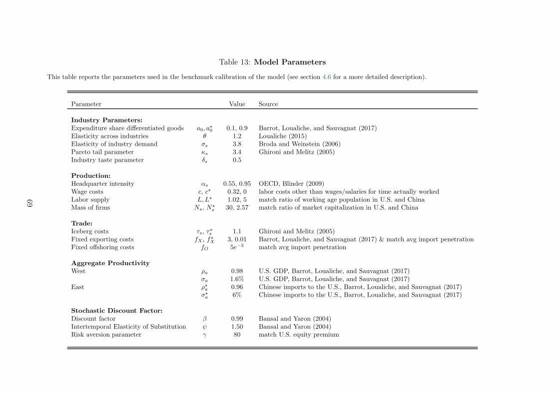
Table 13: Model Parameters

This table reports the parameters used in the benchmark calibration of the model (see section 4.6 for a more detailed description).

Parameter Value Source

Industry Parameters:

Expenditure share differentiated goods a0, a⋆0 0.1, 0.9 Barrot, Loualiche, and Sauvagnat (2017)

Elasticity across industries θ 1.2 Loualiche (2015)Elasticity of industry demand σs 3.8 Broda and Weinstein (2006)Pareto tail parameter κs 3.4 Ghironi and Melitz (2005)Industry taste parameter δs 0.5

Production:

Headquarter intensity αs 0.55, 0.95 OECD, Blinder (2009)Wage costs c, c⋆ 0.32, 0 labor costs other than wages/salaries for time actually workedLabor supply L,L⋆ 1.02, 5 match ratio of working age population in U.S. and ChinaMass of firms Ns, N

⋆s 30, 2.57 match ratio of market capitalization in U.S. and China

Trade:

Iceberg costs τs, τ⋆s 1.1 Ghironi and Melitz (2005)

Fixed exporting costs fX , f⋆X 3, 0.01 Barrot, Loualiche, and Sauvagnat (2017) & match avg import penetration

Fixed offshoring costs fO 5e−3 match avg import penetration

Aggregate Productivity

West ρa 0.98 U.S. GDP, Barrot, Loualiche, and Sauvagnat (2017)σa 1.6% U.S. GDP, Barrot, Loualiche, and Sauvagnat (2017)

East ρ⋆a 0.96 Chinese imports to the U.S., Barrot, Loualiche, and Sauvagnat (2017)σ⋆a 6% Chinese imports to the U.S., Barrot, Loualiche, and Sauvagnat (2017)

Stochastic Discount Factor:

Discount factor β 0.99 Bansal and Yaron (2004)Intertemporal Elasticity of Substitution ψ 1.50 Bansal and Yaron (2004)Risk aversion parameter γ 80 match U.S. equity premium

69

Table 14: Model Simulations: Targeted and Model-Implied Moments

The table reports the main moments of the model-generated data. Panel A tabulates the targeted moments in themodel and the data. The share of the market capitalization (MC) in China is calculated as MCChina/(MCUS +MCChina) and the share of the working age population (WP) in China as WPChina/(WPUS +WPChina). PanelB (C and D) focuses on moments of macroeconomic (industry and financial) quantities. Column titles “Low” and“High” refer to low and high offshorability industries. The model is solved using perturbation methods and isapproximated to the 3rd-order around the deterministic steady state. Moments are calculated based on simulationsover 10’000 periods (with a burn-in period of 1’000 periods).

Panel A: Targeted Moments

model dataShare Market Capitalization China 0.28 0.25Share Working Age Population China 0.17 0.17Avg Import Penetration China - Mean 6.26% 6.36%Avg Import Penetration China - Std 4.08% 2.75%

Panel B: Macro Moments

Agg. Consumption Risk-free Rate Labor Share

model data model data model datamean 2.80% 2.63% 60.54% 58.40%std 9.44% 2.00% 0.27% 2.12%

Panel C: Industry Quantities

Import Penetration Industry Profits

Low High Low Highmean 7.39% 5.36% 0.28 0.32std 5.91% 2.83% 8.14% 3.67%cov( ,A) -0.60 -0.30 0.24 0.12cov( ,A⋆) 5.00 2.48 -1.75 -0.79cov( ,C) -0.51 -0.26 0.76 0.34

Panel D: Asset Prices and Excess Returns

Valuations Excess Returns Export Excess Returns

Low High Low High Low Highmean 10.31 19.96 6.44% 3.53% 8.04% 3.62%std 2.14% 1.65% 16.33% 8.42% 19.07% 9.14%cov( ,A) 0.09 0.06 0.07 0.02 0.13 0.03cov( ,A⋆) -0.43 -0.34 -0.90 -0.31 -1.28 -0.31cov( ,C) 0.20 0.16 0.09 0.03 0.13 0.03

70

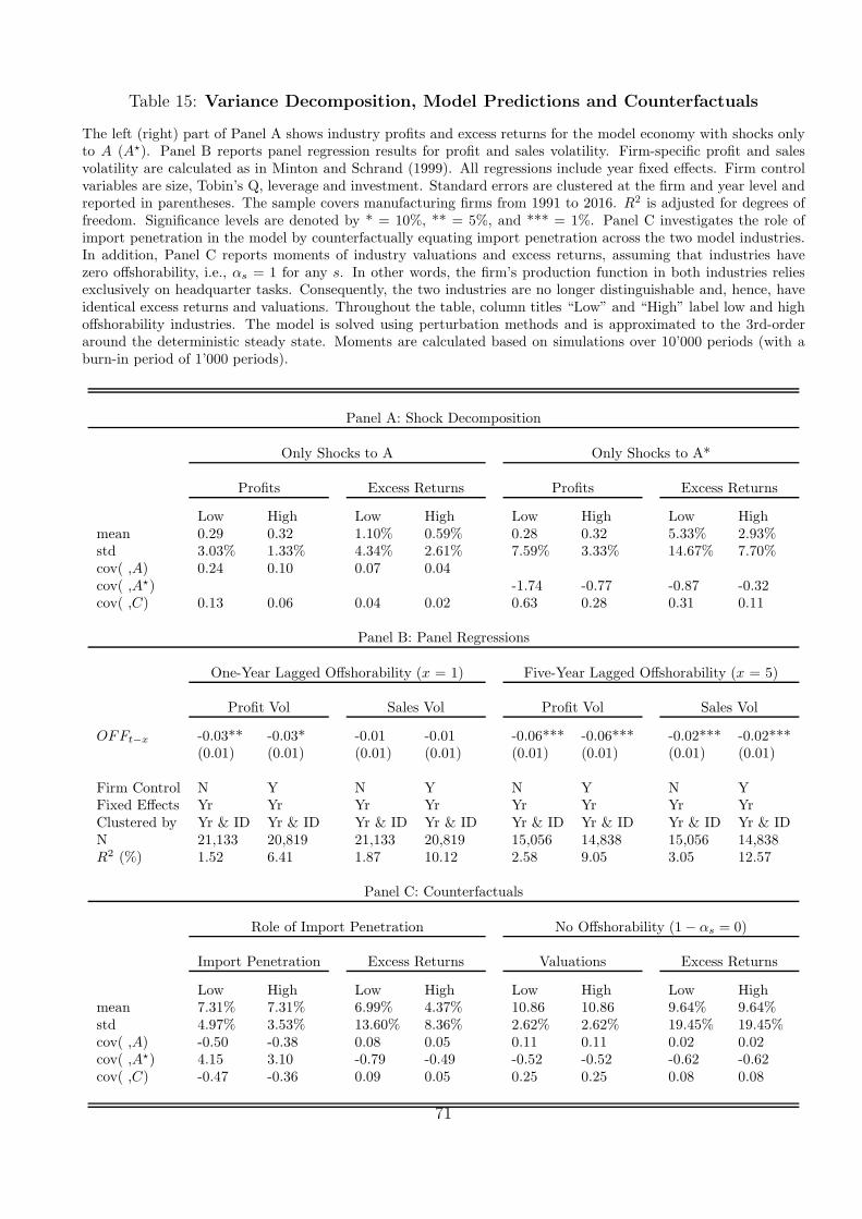
Table 15: Variance Decomposition, Model Predictions and Counterfactuals

The left (right) part of Panel A shows industry profits and excess returns for the model economy with shocks onlyto A (A⋆). Panel B reports panel regression results for profit and sales volatility. Firm-specific profit and salesvolatility are calculated as in Minton and Schrand (1999). All regressions include year fixed effects. Firm controlvariables are size, Tobin’s Q, leverage and investment. Standard errors are clustered at the firm and year level andreported in parentheses. The sample covers manufacturing firms from 1991 to 2016. R2 is adjusted for degrees offreedom. Significance levels are denoted by * = 10%, ** = 5%, and *** = 1%. Panel C investigates the role ofimport penetration in the model by counterfactually equating import penetration across the two model industries.In addition, Panel C reports moments of industry valuations and excess returns, assuming that industries havezero offshorability, i.e., αs = 1 for any s. In other words, the firm’s production function in both industries reliesexclusively on headquarter tasks. Consequently, the two industries are no longer distinguishable and, hence, haveidentical excess returns and valuations. Throughout the table, column titles “Low” and “High” label low and highoffshorability industries. The model is solved using perturbation methods and is approximated to the 3rd-orderaround the deterministic steady state. Moments are calculated based on simulations over 10’000 periods (with aburn-in period of 1’000 periods).

Panel A: Shock Decomposition

Only Shocks to A Only Shocks to A*

Profits Excess Returns Profits Excess Returns

Low High Low High Low High Low Highmean 0.29 0.32 1.10% 0.59% 0.28 0.32 5.33% 2.93%std 3.03% 1.33% 4.34% 2.61% 7.59% 3.33% 14.67% 7.70%cov( ,A) 0.24 0.10 0.07 0.04cov( ,A⋆) -1.74 -0.77 -0.87 -0.32cov( ,C) 0.13 0.06 0.04 0.02 0.63 0.28 0.31 0.11

Panel B: Panel Regressions

One-Year Lagged Offshorability (x = 1) Five-Year Lagged Offshorability (x = 5)

Profit Vol Sales Vol Profit Vol Sales Vol

OFFt−x -0.03** -0.03* -0.01 -0.01 -0.06*** -0.06*** -0.02*** -0.02***(0.01) (0.01) (0.01) (0.01) (0.01) (0.01) (0.01) (0.01)

Firm Control N Y N Y N Y N YFixed Effects Yr Yr Yr Yr Yr Yr Yr YrClustered by Yr & ID Yr & ID Yr & ID Yr & ID Yr & ID Yr & ID Yr & ID Yr & IDN 21,133 20,819 21,133 20,819 15,056 14,838 15,056 14,838R2 (%) 1.52 6.41 1.87 10.12 2.58 9.05 3.05 12.57

Panel C: Counterfactuals

Role of Import Penetration No Offshorability (1− αs = 0)

Import Penetration Excess Returns Valuations Excess Returns

Low High Low High Low High Low Highmean 7.31% 7.31% 6.99% 4.37% 10.86 10.86 9.64% 9.64%std 4.97% 3.53% 13.60% 8.36% 2.62% 2.62% 19.45% 19.45%cov( ,A) -0.50 -0.38 0.08 0.05 0.11 0.11 0.02 0.02cov( ,A⋆) 4.15 3.10 -0.79 -0.49 -0.52 -0.52 -0.62 -0.62cov( ,C) -0.47 -0.36 0.09 0.05 0.25 0.25 0.08 0.08

71

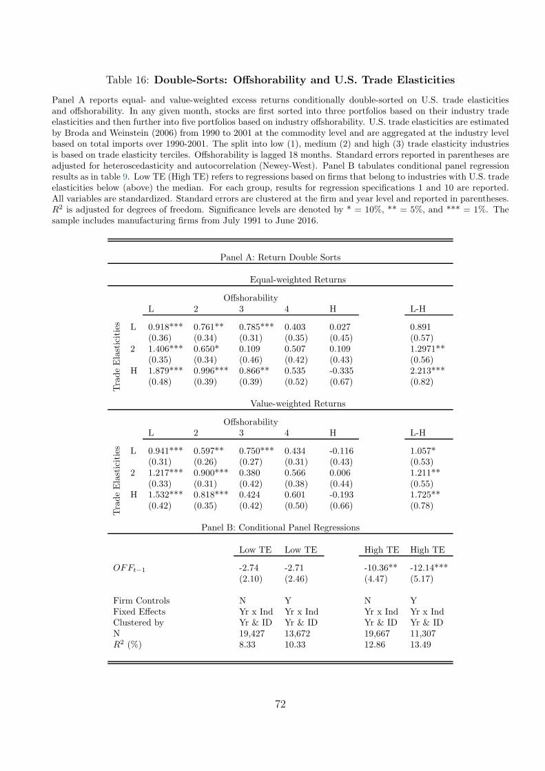
Table 16: Double-Sorts: Offshorability and U.S. Trade Elasticities

Panel A reports equal- and value-weighted excess returns conditionally double-sorted on U.S. trade elasticitiesand offshorability. In any given month, stocks are first sorted into three portfolios based on their industry tradeelasticities and then further into five portfolios based on industry offshorability. U.S. trade elasticities are estimatedby Broda and Weinstein (2006) from 1990 to 2001 at the commodity level and are aggregated at the industry levelbased on total imports over 1990-2001. The split into low (1), medium (2) and high (3) trade elasticity industriesis based on trade elasticity terciles. Offshorability is lagged 18 months. Standard errors reported in parentheses areadjusted for heteroscedasticity and autocorrelation (Newey-West). Panel B tabulates conditional panel regressionresults as in table 9. Low TE (High TE) refers to regressions based on firms that belong to industries with U.S. tradeelasticities below (above) the median. For each group, results for regression specifications 1 and 10 are reported.All variables are standardized. Standard errors are clustered at the firm and year level and reported in parentheses.R2 is adjusted for degrees of freedom. Significance levels are denoted by * = 10%, ** = 5%, and *** = 1%. Thesample includes manufacturing firms from July 1991 to June 2016.

Panel A: Return Double Sorts

Equal-weighted Returns

OffshorabilityL 2 3 4 H L-H

TradeElasticities L 0.918*** 0.761** 0.785*** 0.403 0.027 0.891

(0.36) (0.34) (0.31) (0.35) (0.45) (0.57)2 1.406*** 0.650* 0.109 0.507 0.109 1.2971**

(0.35) (0.34) (0.46) (0.42) (0.43) (0.56)H 1.879*** 0.996*** 0.866** 0.535 -0.335 2.213***

(0.48) (0.39) (0.39) (0.52) (0.67) (0.82)

Value-weighted Returns

OffshorabilityL 2 3 4 H L-H

TradeElasticities L 0.941*** 0.597** 0.750*** 0.434 -0.116 1.057*

(0.31) (0.26) (0.27) (0.31) (0.43) (0.53)2 1.217*** 0.900*** 0.380 0.566 0.006 1.211**

(0.33) (0.31) (0.42) (0.38) (0.44) (0.55)H 1.532*** 0.818*** 0.424 0.601 -0.193 1.725**

(0.42) (0.35) (0.42) (0.50) (0.66) (0.78)

Panel B: Conditional Panel Regressions

Low TE Low TE High TE High TE

OFFt−1 -2.74 -2.71 -10.36** -12.14***(2.10) (2.46) (4.47) (5.17)

Firm Controls N Y N YFixed Effects Yr x Ind Yr x Ind Yr x Ind Yr x IndClustered by Yr & ID Yr & ID Yr & ID Yr & IDN 19,427 13,672 19,667 11,307R2 (%) 8.33 10.33 12.86 13.49

72

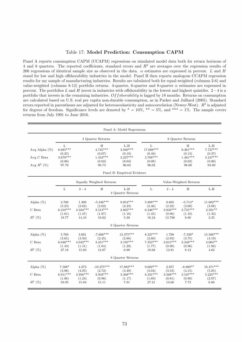
Table 17: Model Prediction: Consumption CAPM

Panel A reports consumption CAPM (CCAPM) regressions on simulated model data both for return horizons of4 and 8 quarters. The reported coefficients, standard errors and R2 are averages over the regression results of200 regressions of identical sample size as observed in the data. α estimates are expressed in percent. L and Hstand for low and high offshorability industries in the model. Panel B then reports analogous CCAPM regressionresults for my sample of manufacturing industries. Results are tabulated both for equal-weighted (columns 2-6) andvalue-weighted (columns 8-12) portfolio returns. 4-quarter, 6-quarter and 8-quarter α estimates are expressed inpercent. The portfolios L and H invest in industries with offshorability in the lowest and highest quintiles. 2−4 is aportfolio that invests in the remaining industries. Offshorability is lagged by 18 months. Returns on consumptionare calculated based on U.S. real per capita non-durable consumption, as in Parker and Julliard (2005). Standarderrors reported in parentheses are adjusted for heteroscedasticity and autocorrelation (Newey-West). R2 is adjustedfor degrees of freedom. Significance levels are denoted by * = 10%, ** = 5%, and *** = 1%. The sample coversreturns from July 1991 to June 2016.

Panel A: Model Regressions

4 Quarter Returns 8 Quarter Returns

L H L-H L H L-HAvg Alpha (%) 8.685*** 4.745*** 3.940*** 17.088*** 9.361*** 7.727***

(0.25) (0.07) (0.19) (0.48) (0.13) (0.37)Avg C Beta 3.679*** 1.452*** 2.227*** 3.708*** 1.461*** 2.247***

(0.06) (0.02) (0.04) (0.08) (0.02) (0.06)Avg R2 (%) 97.79 98.73 96.62 96.02 98.00 93.80

Panel B: Empirical Evidence

Equally Weighted Returns Value-Weighted Returns

L 2 - 4 H L-H L 2 - 4 H L-H4 Quarter Returns

Alpha (%) 3.708 1.309 -5.346*** 9.054*** 5.888*** 0.605 -5.714* 11.602***(3.23) (2.62) (2.02) (2.23) (2.46) (2.22) (3.00) (3.08)

C Beta 6.318*** 4.334*** 3.513*** 2.805*** 6.346*** 3.833*** 3.755*** 2.591**(1.61) (1.47) (1.07) (1.16) (1.45) (0.96) (1.10) (1.32)

R2 (%) 19.77 14.10 10.62 5.30 16.24 13.790 8.80 2.35

6 Quarter Returns

Alpha (%) 5.769 3.061 -7.606*** 13.375*** 8.227*** 1.798 -7.339* 15.566***(3.65) (3.50) (2.45) (2.88) (2.60) (2.93) (3.75) (4.19)

C Beta 6.646*** 4.042*** 3.451*** 3.195*** 7.352*** 3.615*** 3.348*** 4.004**(1.43) (1.41) (1.04) (1.20) (1.77) (0.90) (0.96) (1.86)

R2 (%) 27.18 15.03 12.87 6.90 19.68 13.81 8.12 4.62

8 Quarter Returns

Alpha (%) 7.508* 4.273 -10.375*** 17.882*** 9.602*** 2.957 -8.869** 18.471***(3.96) (4.05) (2.72) (3.49) (3.04) (3.53) (4.15) (5.05)

C Beta 6.911*** 3.956*** 3.503*** 3.408*** 8.331*** 3.568*** 3.107*** 5.225***(1.06) (1.24) (0.96) (1.17) (1.69) (0.81) (0.80) (2.07)

R2 (%) 33.95 15.94 15.11 7.91 27.21 13.66 7.73 6.86

73

Online Appendix to “From Local to Global:

Offshoring and Asset Prices”

Lorenzo Bretscher

LSE∗

This online appendix contains additional information on the sample and data construction (section 1), and

on the OES data set and the industry offshorability index across sectors (section 2), further robustness

tests of the empirical results of the paper (section 3) and details about the computational approach

employed to solve the model (section 4).

1 Sample Construction and Variable Definition

Monthly common stock data is from the Center for Research in Security Prices (CRSP share code SHRCD

= 10 or 11). The sample includes stocks listed on NYSE, AMEX, and NASDAQ (exchcd = 1 or 2 or

3). Accounting information is from Standard and Poor’s Compustat annual industrial files. I follow the

literature and exclude from my sample firms with primary standard industrial classifications between 4900

and 4999 (regulated firms) and between 6000 and 6999 (financial firms). Following Zhang (2016), the

firm-level accounting variables and size measures are winsorized at the 1% level to reduce the influence

of possible outliers.

I construct the following variables for every firm:

• Assets is the logarithm of a firm’s total book assets (AT).

• Cash is a firm’s cash holdings defined as cash and short-term investments (CHE) scaled by total

book assets (AT).

• Q is a firm’s Tobin’s Q defined as total book assets (AT) minus common equity (CEQ) plus the

market value of equity scaled by total assets (AT) following Dasgupta, Noe, and Wang (2011).

• PP&E is net property, plant and investment (PPENT) scaled by total book assets (AT).

• Size and BooktoMarket are calculated following Fama and French (1992).

∗Department of Finance, Email: l.p.bretscher@lse.ac.uk

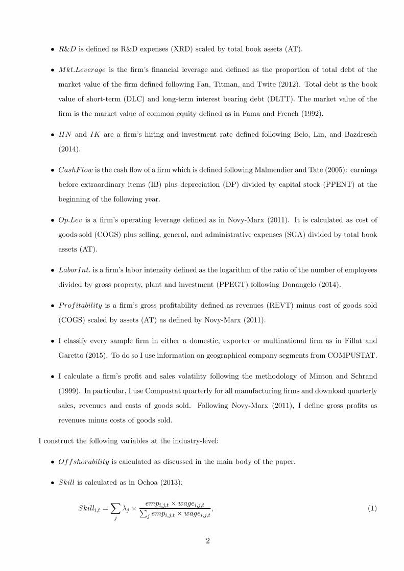
• R&D is defined as R&D expenses (XRD) scaled by total book assets (AT).

• Mkt.Leverage is the firm’s financial leverage and defined as the proportion of total debt of the

market value of the firm defined following Fan, Titman, and Twite (2012). Total debt is the book

value of short-term (DLC) and long-term interest bearing debt (DLTT). The market value of the

firm is the market value of common equity defined as in Fama and French (1992).

• HN and IK are a firm’s hiring and investment rate defined following Belo, Lin, and Bazdresch

(2014).

• CashF low is the cash flow of a firm which is defined following Malmendier and Tate (2005): earnings

before extraordinary items (IB) plus depreciation (DP) divided by capital stock (PPENT) at the

beginning of the following year.

• Op.Lev is a firm’s operating leverage defined as in Novy-Marx (2011). It is calculated as cost of

goods sold (COGS) plus selling, general, and administrative expenses (SGA) divided by total book

assets (AT).

• LaborInt. is a firm’s labor intensity defined as the logarithm of the ratio of the number of employees

divided by gross property, plant and investment (PPEGT) following Donangelo (2014).

• Profitability is a firm’s gross profitability defined as revenues (REVT) minus cost of goods sold

(COGS) scaled by assets (AT) as defined by Novy-Marx (2011).

• I classify every sample firm in either a domestic, exporter or multinational firm as in Fillat and

Garetto (2015). To do so I use information on geographical company segments from COMPUSTAT.

• I calculate a firm’s profit and sales volatility following the methodology of Minton and Schrand

(1999). In particular, I use Compustat quarterly for all manufacturing firms and download quarterly

sales, revenues and costs of goods sold. Following Novy-Marx (2011), I define gross profits as

revenues minus costs of goods sold.

I construct the following variables at the industry-level:

• Offshorability is calculated as discussed in the main body of the paper.

• Skill is calculated as in Ochoa (2013):

Skilli,t =∑

j

λj ×empi,j,t ×wagei,j,t

∑

j empi,j,t × wagei,j,t, (1)

2

where λj is the skill-level of occupation j. λj is the “job zone” of a given occupation which ranges

between one and five.

• Routine is calculated as follows:

Routinei,t =∑

j

1routinej>routinep66 × routinej ×empi,j,t × wagei,j,t

∑

j empi,j,t × wagei,j,t, (2)

where routinej is the routine task score for occupation j which is calculated using task level content

from O*NET as in Acemoglu and Autor (2011).

• Shipping Costs are calculated following Barrot, Loualiche, and Sauvagnat (2017).

• Value Share of Imports and Import Penetration are calculated following Bernard, Jensen, and Schott

(2006). The value share of imports from low wage countries, for example, is calculated as the total

imports from low wage countries in an industry divided by the total imports in the same industry.

Import penetration by low wage countries of a given industry i at time t is calculated as follows:

LWPENi,t =( V L

i,t

Vi,t +Qi,t −Xi,t

)

,

where V Li,t and Vi,t represent the value of imports from low wage countries and all countries, respec-

tively, Qi,t is domestic production, and Xi,t represents US exports.

2 OES Data and Industry Offshorability across Sectors

While the OES survey methodology is designed to create detailed cross-sectional employment and wage

estimates for the U.S., States, metropolitan and nonmetropolitan areas, across industry and by industry,

comparisons of two or more points in time might be difficult. The time-series interpretation of OES data

might be misleading due to various changes in the construction of the data over time such as changes

in the occupational and industrial classification. The nature of these changes are summarized on the

webpage of the Bureau of Labor Statistics as follows:

(Excerpts were downloaded on October 10, 2017 from https://www.bls.gov/oes/oes ques.htm)

Changes in occupational classification: The OES survey used its own occupational classification

system through 1998. The 1999 OES survey data provide estimates for most of the nonresidual occupations

in the 2000 Standard Occupational Classification (SOC) system. The 2004-2009 OES data provides

estimates for all occupations in the 2000 SOC. The May 2010 data provides estimates for most occupations

3

in the 2010 SOC (for more on the 2010 occupations, see below). Because of these changes, it may

be difficult to compare some occupations even if they are found in both classification systems. For

example, both the old OES system and the 2000 SOC include the occupation ”computer programmers.”

However, estimates for this occupation may not be comparable over time because the 2000 SOC has

several computer-related occupations that were not included in the older classification system. Workers

in newly classified occupations, such as systems software engineers and applications software engineers,

may have been reported as computer programmers in the past. Therefore, even occupations that appear

the same in the two systems may show employment shifts due to the addition or deletion of related

occupations.

Changes in industrial classification: In 2002, the OES survey switched from the Standard Indus-

trial Classification (SIC) system to the North American Industry Classification System (NAICS). As a

result, there were changes in many industry definitions. Even definitions that appear similar between the

two industry classifications may have differences because of the way auxiliary establishments are treated.

For example, under SIC the industry ”grocery stores” included their retail establishments, warehouses,

transportation facilities, and administrative headquarters. Under NAICS, the four establishment types

would be reported in separate industries. Only the retail establishments would be included in the NAICS

industry for ”grocery stores.” The change in industrial classification also resulted in changes to the oc-

cupations listed on the survey form for a given industry. In 2008, the OES survey switched to the 2007

NAICS classification system from the 2002 NAICS. The most significant revisions are in the Information

Sector, particularly within the Telecommunications area. Beginning in 2010, Tennessee Valley Authority

(TVA) data is included in the Federal Government estimates.

While the main paper shows rankings of industry offshorability for manufacturing and services sep-

arately, table A2 reports corresponding rankings across all industries. In 1992, the industries with the

highest offshoring potential were almost exclusively manufacturing industries whereas the bottom indus-

tries feature mining industries. In 2015, the industry ranking looks very different. Industries among

the top ten are by no means only related to manufacturing. The bottom industries, however, do not

seem to have drastically changed in their nature compared to 1992. Interestingly, the top ten in 2015

are mostly service industries which is consistent with Jensen (2011), Blinder (2009) and Amiti and Wei

(2009) who discuss that recent advances in communication technologies increasingly allow for offshoring

of service industry jobs. Moreover, this change over time is in line with recent papers which document

that offshoring and replacement of offshorable jobs with imports have led to a substantial decrease in

4

manufacturing employment over the recent past.∗ This can be seen from figure A1 which plots a strongly

negative relationship between U.S. imports as percentage of GDP and the manufacturing employment

share. As a result of this, one would expect that the manufacturing sector becomes relatively less off-

shorable compared with services over time. Given that the rankings within manufacturing and services

are very persistent over time, the drastic change in top ten industries in 1992 and 2015 is likely to be due

to structural changes across sectors, i.e. services and manufacturing.

Yet another way to look at this sectoral change in offshorability over time is to plot cross-sectional

correlations of industry offshorability and industry routine-task labor and skill at different points in time.

The results are plotted in figure A2. While offshorability and routine are significantly and positively

correlated at the beginning of the sample, the correlation coefficients decrease continuously from 1997

onwards. This pattern is not due to wage-weighting when constructing the offshorability index. The

correlations look almost identical for the OFF ⋆i,t measure that does not rely on wages (right panel in

figure A2). The sudden drop in correlation in 2001 coincides with the sharp decrease in routine-labor in

the U.S. documented by Zhang (2016) and the decrease in manufacturing employment which was fueled

by China’s admission to the World Trade Organization (WTO) in 2001 as discussed in Autor, Dorn, and

Hanson (2016).

Finally, figure A3 reports additional evidence on the importance of China for the U.S. trade deficit

in goods. The left panel plots the U.S. trade balance in goods when considering all countries (solid blue

line) and China only (red solid line). The importance of trades with China for the overall trade balance

are striking. In the year 2009, 44.5% of the U.S. trade deficit in goods was due to trades with China.

Interestingly, the right panel of figure A3 shows the trade balance in goods for the U.S. and China,

respectively. Consistent with the interpretation of comparative advantage, the U.S. and Chinese trade

balances in goods look like a mirror image. Of course, this is at best suggestive evidence because the

countries potentially trade with many other countries, i.e. have various and heterogenous trade partners.

3 Robustness: Asset Pricing Results

This section delivers further robustness tests for the asset pricing results in the main paper. Table A3

reports regression results across all industries for the unconditional (Panel A) and conditional CAPM

(Panel B) as well as the Fama and French (1993) three factor model (Panel C).

Table A4 splits the sample into manufacturing and services industries and reports regression results

∗See among others Autor, Dorn, and Hanson (2013), Acemoglu, Autor, Dorn, Hanson, and Price (2016) andAutor, Dorn, and Hanson (2016).

5

for the Fama and French (1993) three factor model.

Table A5 reports univariate returns both for the full as well as for various subsamples. In this

robustness test I keep the ranking of industry offshorability fixed over time. In other words, for the

period between 1991 and 2002, I keep the industry offshorability fixed at the values for 1990, and for

the period from 2002 to 2016, I fix offshorability at the values from the year 2001. Hence, I simply fix

offshorability at the first observation available for the two industry classification regimes in the OES data

(as discussed above).

Table A6 shows robustness tests for the predictability regressions of the main paper. Panel A and

B report regression results for manufacturing and services for different industry definitions. While the

baseline specification uses industry×year fixed effects based on 17 industries as defined in Fama and

French (1988), I assess the robustness of the results for 49 industries as defined in Fama and French

(1997), industries defined by one and two digit SIC codes as well as with only year fixed effects.

Table A7 shows monthly excess return double sorts on import penetration from China and offshora-

bility. The results are very similar to the double sorts on import penetration from low-wage countries and

offshorability.

Finally, tables A8 and A9 report factor model regression results which control for the globalization

risk premium as defined in Barrot, Loualiche, and Sauvagnat (2017) and factors based on foreign exchange

exposure from Lustig, Roussanov, and Verdelhan (2011) and Verdelhan (2017).

4 Computational Approach

The model is solved using perturbation methods around the steady-state. In particular, I use third-order

approximations of the policy function around the deterministic steady-state of the model. I then simulate

the model for 11’000 periods. I disregard the first 1’000 periods as a so-called burn-in period. Based

on the remaining 10’000 periods of simulated data, I calculate moments for different model quantities.

Impulse response functions are calculated as the response of a model quantity with respect to a one

standard deviation shocks of either A or A⋆ (or τ⋆ for the counterfactual analysis on trade costs). The

plotted IRFs are calculated as the mean over 500 simulated IRFs.

6

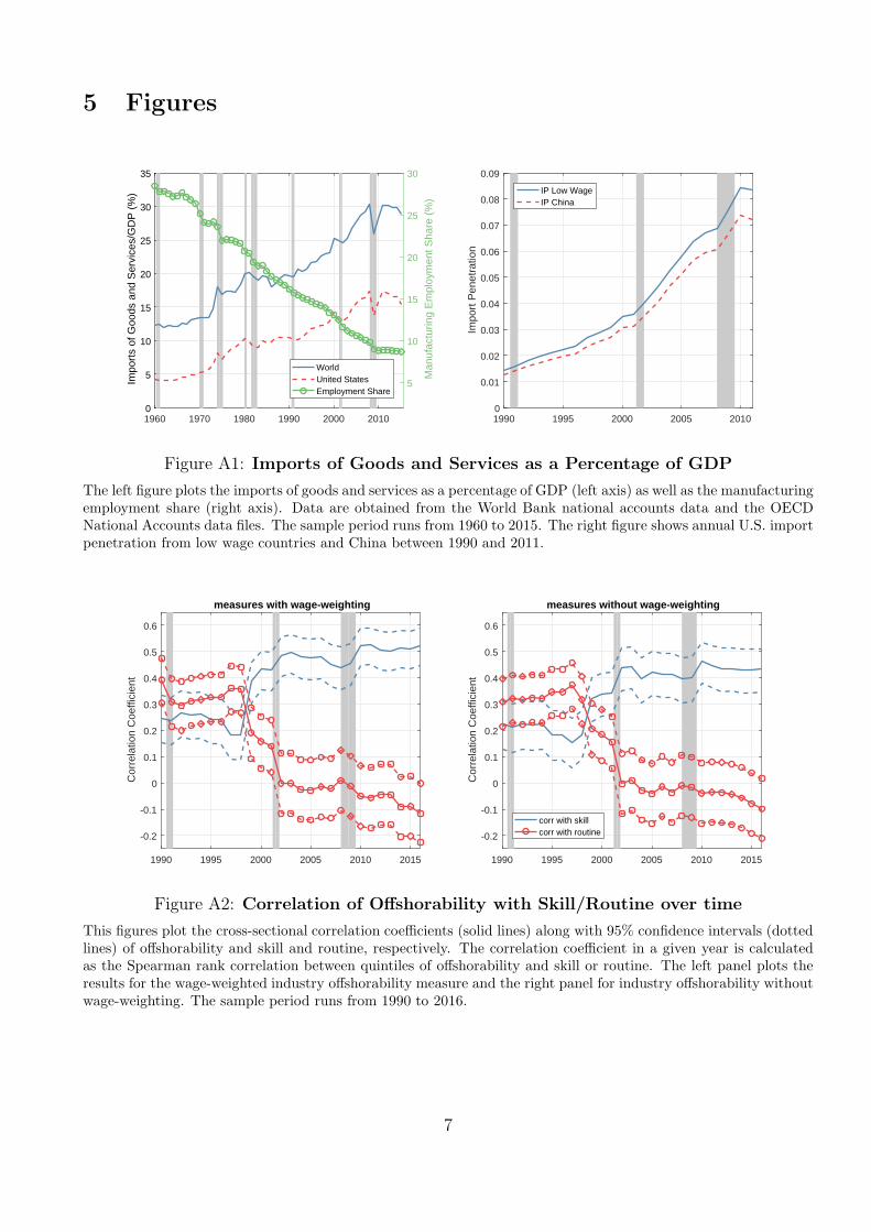
5 Figures

1960 1970 1980 1990 2000 20100

5

10

15

20

25

30

35

Impo

rts

of G

oods

and

Ser

vice

s/G

DP

(%

)

5

10

15

20

25

30

Man

ufac

turin

g E

mpl

oym

ent S

hare

(%

)

WorldUnited StatesEmployment Share

1990 1995 2000 2005 20100

0.01

0.02

0.03

0.04

0.05

0.06

0.07

0.08

0.09

Impo

rt P

enet

ratio

n

IP Low WageIP China

Figure A1: Imports of Goods and Services as a Percentage of GDP

The left figure plots the imports of goods and services as a percentage of GDP (left axis) as well as the manufacturingemployment share (right axis). Data are obtained from the World Bank national accounts data and the OECDNational Accounts data files. The sample period runs from 1960 to 2015. The right figure shows annual U.S. importpenetration from low wage countries and China between 1990 and 2011.

1990 1995 2000 2005 2010 2015

-0.2

-0.1

0

0.1

0.2

0.3

0.4

0.5

0.6

Cor

rela

tion

Coe

ffici

ent

measures with wage-weighting

1990 1995 2000 2005 2010 2015

-0.2

-0.1

0

0.1

0.2

0.3

0.4

0.5

0.6

Cor

rela

tion

Coe

ffici

ent

measures without wage-weighting

corr with skillcorr with routine

Figure A2: Correlation of Offshorability with Skill/Routine over time

This figures plot the cross-sectional correlation coefficients (solid lines) along with 95% confidence intervals (dottedlines) of offshorability and skill and routine, respectively. The correlation coefficient in a given year is calculatedas the Spearman rank correlation between quintiles of offshorability and skill or routine. The left panel plots theresults for the wage-weighted industry offshorability measure and the right panel for industry offshorability withoutwage-weighting. The sample period runs from 1990 to 2016.

7

1960 1970 1980 1990 2000 2010-900

-800

-700

-600

-500

-400

-300

-200

-100

0

U.S

. Tra

de B

alan

ces

in G

oods

in B

illio

ns o

f 200

9 D

olla

rs

Goods: OverallGoods: China

1960 1970 1980 1990 2000 2010

-800

-600

-400

-200

0

200

400

Tra

de B

alan

ces

in G

oods

in B

illio

ns o

f 200

9 D

olla

rs

U.S.China

Figure A3: Trade Balances in Goods

The left panel plots the U.S. trade balances (i.e. exports minus imports) in goods in 2009 Dollars. The blue solidline refers to the overall trade balance in goods. In other words, trades between the U.S. and any other country areconsidered. On the other hand, the red solid line plots the U.S. trade balance in goods with China only. The rightpanel plots the overall trade balance in goods both for the U.S. and China. Data are obtained from the Bureau ofEconomic Analysis. The sample period runs from 1960 to 2016.

8

6 Tables

Table A1: Occupation Tasks that define Offshorability

This table tabulates the tasks used to calculate occupation offshorability by Firpo, Fortin, and Lemieux (2013).The acronyms WA and WC in the third column stand for work activity and work context.

Firpo, Fortin and Lemieux (2013)

Face-to-Face Contact

4.C.1.a.2.l Face-to-Face Discussions WC4.A.4.a.4 Establishing and Maintaining Interpersonal Relationships WA4.A.4.a.5 Assisting and Caring for Others WA4.A.4.a.8 Performing for or Working Directly with the Public WA4.A.4.b.5 Coaching and Developing Others WA

On-site

4.A.1.b.2 Inspecting Equipment, Structures, or Material WA4.A.3.a.2 Handling and Moving Objects WA4.A.3.a.3 Controlling Machines and Processes WA4.A.3.a.4 Operating Vehicles, Mechanized Devices, or Equipment WA4.A.3.b.4 Repairing and Maintaining Mechanical Equipment (*0.5) WA4.A.3.b.5 Repairing and Maintaining Electronic Equipment (*0.5) WA

Decision-Making

4.A.2.b.1 Making Decisions and Solving Problems WA4.A.2.b.2 Thinking Creatively WA4.A.2.b.4 Developing Objectives and Solving Problems WC4.C.1.c.2 Responsibility for Outcomes and Results WC4.C.3.a.2.b Frequency of Decision Making

9

Table A2: Most Offshorable and Non-Offshorable Industries

Panels A and B tabulate the top and bottom ten industries in terms of their offshoring potential, OFFi,t, for the years 1992 and 2015, respectively. Industriesare defined at the three-digit SIC level until 2001 and at the four-digit NAICS level thereafter.

Panel A: 1992 - Top and Bottom Ten Industries by Offshorability

SIC Industry Title OFFi,t SIC Industry Title OFFi,t

8720 Accounting, Auditing, and Bookkeeping Services 2.419 8650 Political Organizations -2.1742310 Men’s and Boys’ Suits, Coats, and Overcoats 2.392 8620 Professional Membership Organizations -2.2137250 Shoe Repair Shops and Shoeshine Parlors 2.257 3760 Guided Missiles and Space Vehicles and Parts -2.2542320 Men’s and Boys’ Furnishings, Work Clothing, and Allied Garments 2.141 3660 Communications Equipment -2.4302360 Girls’, Children’s, and Infants’ Outerwear 2.120 8730 Research, Development, and Testing Services -2.4382330 Women’s, Misses’, and Juniors’ Outerwear 1.921 8630 Labor Unions and Similar Labor Organizations -2.6312340 Women’s, Misses’, Children’s, and Infants’ Undergarments 1.759 1060 Ferroalloy Ores, Except Vanadium -2.7152340 Hats, Caps, and Millinery 1.649 4820 Telegraph Communication -2.8273150 Leather Gloves and Mittens 1.543 3810 Aeronautical and Nautical Systems -3.0192380 Miscellaneous Apparel and Accessories 1.541 1230 Anthracite Mining -3.843

Panel B: 2015 - Top and Bottom Ten Industries by Offshorability

NAICS Industry Title OFFi,t NAICS Industry Title OFFi,t

511200 Software Publishers 3.240 237100 Nonscheduled Air Transportation -1.307541200 Acccounting, Tax Preparation, Bookkeeping, and Payroll Services 3.150 483200 Utility System Construction -1.307519100 Other Information Services 3.057 485500 Inland Water Transportation -1.336541500 Compuer Systems Design and Related Services 3.017 481100 Charter Bus Industry -1.397523900 Other Financial Activities 2.901 487900 Scenic and Sightseeing Transportation -1.425334100 Computer and Peripheral Equipment Manufacturing 2.521 212100 Coal Mining -1.458518200 Data Processing, Hosting, and Related Services 2.473 485200 Interurban and Rural Bus Transportation -1.604541100 Legal Services 2.470 485100 Urban Transport Sytems -1.612524100 Insurance Carriers 2.450 621200 Offices of Dentists -1.706511100 Newspaper, Periodical, Book, and Directory Publishers 2.346 621900 Other Ambulatory Health Care Services -1.948

10

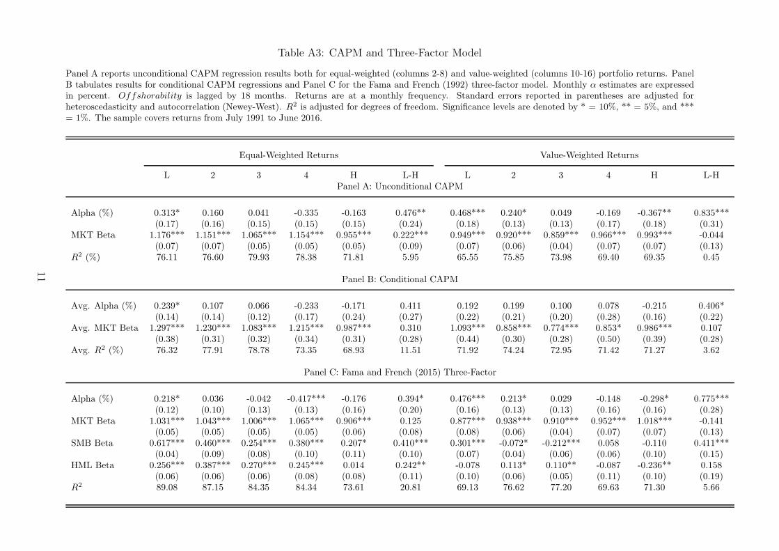
Table A3: CAPM and Three-Factor Model

Panel A reports unconditional CAPM regression results both for equal-weighted (columns 2-8) and value-weighted (columns 10-16) portfolio returns. PanelB tabulates results for conditional CAPM regressions and Panel C for the Fama and French (1992) three-factor model. Monthly α estimates are expressedin percent. Offshorability is lagged by 18 months. Returns are at a monthly frequency. Standard errors reported in parentheses are adjusted forheteroscedasticity and autocorrelation (Newey-West). R2 is adjusted for degrees of freedom. Significance levels are denoted by * = 10%, ** = 5%, and ***= 1%. The sample covers returns from July 1991 to June 2016.

Equal-Weighted Returns Value-Weighted Returns

L 2 3 4 H L-H L 2 3 4 H L-HPanel A: Unconditional CAPM

Alpha (%) 0.313* 0.160 0.041 -0.335 -0.163 0.476** 0.468*** 0.240* 0.049 -0.169 -0.367** 0.835***(0.17) (0.16) (0.15) (0.15) (0.15) (0.24) (0.18) (0.13) (0.13) (0.17) (0.18) (0.31)

MKT Beta 1.176*** 1.151*** 1.065*** 1.154*** 0.955*** 0.222*** 0.949*** 0.920*** 0.859*** 0.966*** 0.993*** -0.044(0.07) (0.07) (0.05) (0.05) (0.05) (0.09) (0.07) (0.06) (0.04) (0.07) (0.07) (0.13)

R2 (%) 76.11 76.60 79.93 78.38 71.81 5.95 65.55 75.85 73.98 69.40 69.35 0.45

Panel B: Conditional CAPM

Avg. Alpha (%) 0.239* 0.107 0.066 -0.233 -0.171 0.411 0.192 0.199 0.100 0.078 -0.215 0.406*(0.14) (0.14) (0.12) (0.17) (0.24) (0.27) (0.22) (0.21) (0.20) (0.28) (0.16) (0.22)

Avg. MKT Beta 1.297*** 1.230*** 1.083*** 1.215*** 0.987*** 0.310 1.093*** 0.858*** 0.774*** 0.853* 0.986*** 0.107(0.38) (0.31) (0.32) (0.34) (0.31) (0.28) (0.44) (0.30) (0.28) (0.50) (0.39) (0.28)

Avg. R2 (%) 76.32 77.91 78.78 73.35 68.93 11.51 71.92 74.24 72.95 71.42 71.27 3.62

Panel C: Fama and French (2015) Three-Factor

Alpha (%) 0.218* 0.036 -0.042 -0.417*** -0.176 0.394* 0.476*** 0.213* 0.029 -0.148 -0.298* 0.775***(0.12) (0.10) (0.13) (0.13) (0.16) (0.20) (0.16) (0.13) (0.13) (0.16) (0.16) (0.28)

MKT Beta 1.031*** 1.043*** 1.006*** 1.065*** 0.906*** 0.125 0.877*** 0.938*** 0.910*** 0.952*** 1.018*** -0.141(0.05) (0.05) (0.05) (0.05) (0.06) (0.08) (0.08) (0.06) (0.04) (0.07) (0.07) (0.13)

SMB Beta 0.617*** 0.460*** 0.254*** 0.380*** 0.207* 0.410*** 0.301*** -0.072* -0.212*** 0.058 -0.110 0.411***(0.04) (0.09) (0.08) (0.10) (0.11) (0.10) (0.07) (0.04) (0.06) (0.06) (0.10) (0.15)

HML Beta 0.256*** 0.387*** 0.270*** 0.245*** 0.014 0.242** -0.078 0.113* 0.110** -0.087 -0.236** 0.158(0.06) (0.06) (0.06) (0.08) (0.08) (0.11) (0.10) (0.06) (0.05) (0.11) (0.10) (0.19)

R2 89.08 87.15 84.35 84.34 73.61 20.81 69.13 76.62 77.20 69.63 71.30 5.66

11

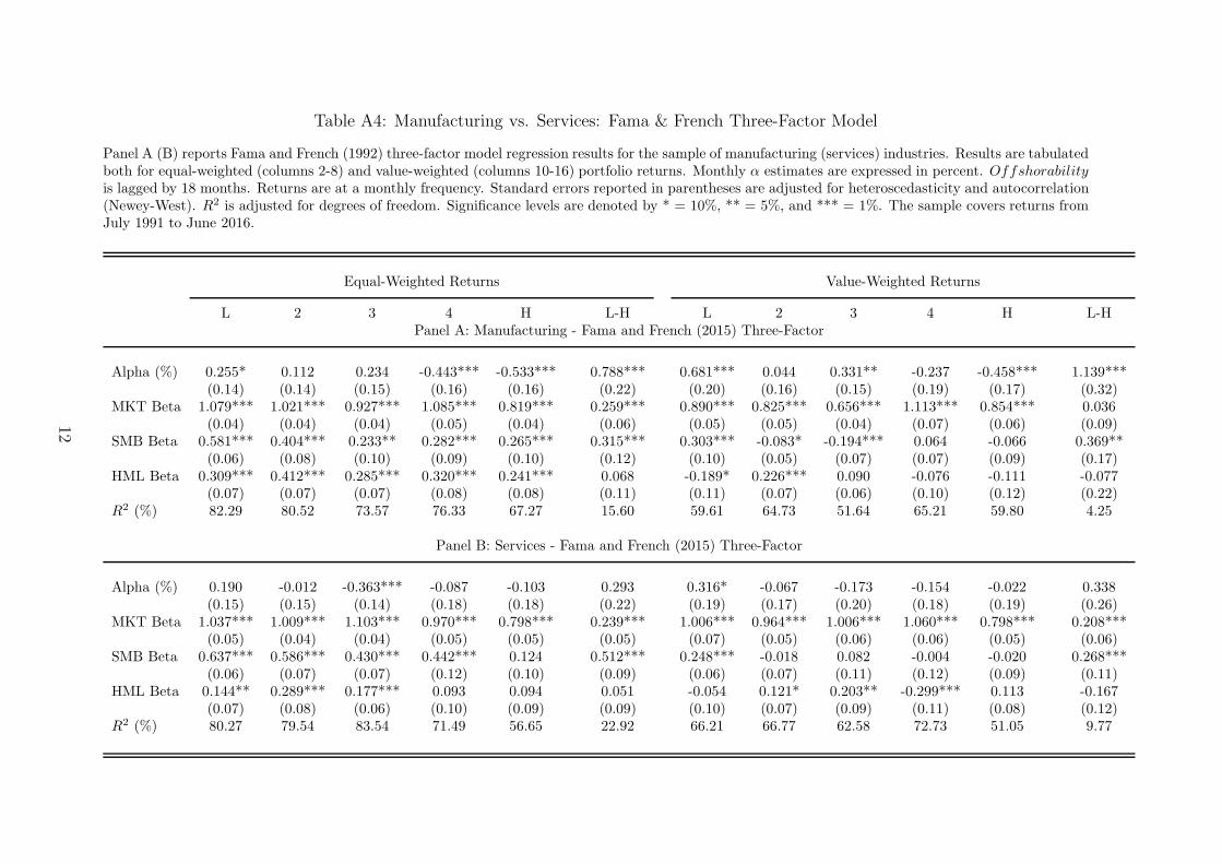
Table A4: Manufacturing vs. Services: Fama & French Three-Factor Model

Panel A (B) reports Fama and French (1992) three-factor model regression results for the sample of manufacturing (services) industries. Results are tabulatedboth for equal-weighted (columns 2-8) and value-weighted (columns 10-16) portfolio returns. Monthly α estimates are expressed in percent. Offshorability

is lagged by 18 months. Returns are at a monthly frequency. Standard errors reported in parentheses are adjusted for heteroscedasticity and autocorrelation(Newey-West). R2 is adjusted for degrees of freedom. Significance levels are denoted by * = 10%, ** = 5%, and *** = 1%. The sample covers returns fromJuly 1991 to June 2016.

Equal-Weighted Returns Value-Weighted Returns

L 2 3 4 H L-H L 2 3 4 H L-HPanel A: Manufacturing - Fama and French (2015) Three-Factor

Alpha (%) 0.255* 0.112 0.234 -0.443*** -0.533*** 0.788*** 0.681*** 0.044 0.331** -0.237 -0.458*** 1.139***(0.14) (0.14) (0.15) (0.16) (0.16) (0.22) (0.20) (0.16) (0.15) (0.19) (0.17) (0.32)

MKT Beta 1.079*** 1.021*** 0.927*** 1.085*** 0.819*** 0.259*** 0.890*** 0.825*** 0.656*** 1.113*** 0.854*** 0.036(0.04) (0.04) (0.04) (0.05) (0.04) (0.06) (0.05) (0.05) (0.04) (0.07) (0.06) (0.09)

SMB Beta 0.581*** 0.404*** 0.233** 0.282*** 0.265*** 0.315*** 0.303*** -0.083* -0.194*** 0.064 -0.066 0.369**(0.06) (0.08) (0.10) (0.09) (0.10) (0.12) (0.10) (0.05) (0.07) (0.07) (0.09) (0.17)

HML Beta 0.309*** 0.412*** 0.285*** 0.320*** 0.241*** 0.068 -0.189* 0.226*** 0.090 -0.076 -0.111 -0.077(0.07) (0.07) (0.07) (0.08) (0.08) (0.11) (0.11) (0.07) (0.06) (0.10) (0.12) (0.22)

R2 (%) 82.29 80.52 73.57 76.33 67.27 15.60 59.61 64.73 51.64 65.21 59.80 4.25

Panel B: Services - Fama and French (2015) Three-Factor

Alpha (%) 0.190 -0.012 -0.363*** -0.087 -0.103 0.293 0.316* -0.067 -0.173 -0.154 -0.022 0.338(0.15) (0.15) (0.14) (0.18) (0.18) (0.22) (0.19) (0.17) (0.20) (0.18) (0.19) (0.26)

MKT Beta 1.037*** 1.009*** 1.103*** 0.970*** 0.798*** 0.239*** 1.006*** 0.964*** 1.006*** 1.060*** 0.798*** 0.208***(0.05) (0.04) (0.04) (0.05) (0.05) (0.05) (0.07) (0.05) (0.06) (0.06) (0.05) (0.06)

SMB Beta 0.637*** 0.586*** 0.430*** 0.442*** 0.124 0.512*** 0.248*** -0.018 0.082 -0.004 -0.020 0.268***(0.06) (0.07) (0.07) (0.12) (0.10) (0.09) (0.06) (0.07) (0.11) (0.12) (0.09) (0.11)

HML Beta 0.144** 0.289*** 0.177*** 0.093 0.094 0.051 -0.054 0.121* 0.203** -0.299*** 0.113 -0.167(0.07) (0.08) (0.06) (0.10) (0.09) (0.09) (0.10) (0.07) (0.09) (0.11) (0.08) (0.12)

R2 (%) 80.27 79.54 83.54 71.49 56.65 22.92 66.21 66.77 62.58 72.73 51.05 9.77

12

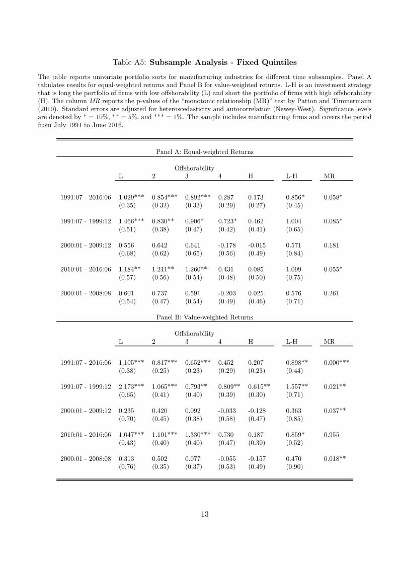
Table A5: Subsample Analysis - Fixed Quintiles

The table reports univariate portfolio sorts for manufacturing industries for different time subsamples. Panel Atabulates results for equal-weighted returns and Panel B for value-weighted returns. L-H is an investment strategythat is long the portfolio of firms with low offshorability (L) and short the portfolio of firms with high offshorability(H). The column MR reports the p-values of the “monotonic relationship (MR)” test by Patton and Timmermann(2010). Standard errors are adjusted for heteroscedasticity and autocorrelation (Newey-West). Significance levelsare denoted by * = 10%, ** = 5%, and *** = 1%. The sample includes manufacturing firms and covers the periodfrom July 1991 to June 2016.

Panel A: Equal-weighted Returns

OffshorabilityL 2 3 4 H L-H MR

1991:07 - 2016:06 1.029*** 0.854*** 0.892*** 0.287 0.173 0.856* 0.058*(0.35) (0.32) (0.33) (0.29) (0.27) (0.45)

1991:07 - 1999:12 1.466*** 0.830** 0.906* 0.723* 0.462 1.004 0.085*(0.51) (0.38) (0.47) (0.42) (0.41) (0.65)

2000:01 - 2009:12 0.556 0.642 0.641 -0.178 -0.015 0.571 0.181(0.68) (0.62) (0.65) (0.56) (0.49) (0.84)

2010:01 - 2016:06 1.184** 1.211** 1.260** 0.431 0.085 1.099 0.055*(0.57) (0.56) (0.54) (0.48) (0.50) (0.75)

2000:01 - 2008:08 0.601 0.737 0.591 -0.203 0.025 0.576 0.261(0.54) (0.47) (0.54) (0.49) (0.46) (0.71)

Panel B: Value-weighted Returns

OffshorabilityL 2 3 4 H L-H MR

1991:07 - 2016:06 1.105*** 0.817*** 0.652*** 0.452 0.207 0.898** 0.000***(0.38) (0.25) (0.23) (0.29) (0.23) (0.44)

1991:07 - 1999:12 2.173*** 1.065*** 0.793** 0.809** 0.615** 1.557** 0.021**(0.65) (0.41) (0.40) (0.39) (0.30) (0.71)

2000:01 - 2009:12 0.235 0.420 0.092 -0.033 -0.128 0.363 0.037**(0.70) (0.45) (0.38) (0.58) (0.47) (0.85)

2010:01 - 2016:06 1.047*** 1.101*** 1.330*** 0.730 0.187 0.859* 0.955(0.43) (0.40) (0.40) (0.47) (0.30) (0.52)

2000:01 - 2008:08 0.313 0.502 0.077 -0.055 -0.157 0.470 0.018**(0.76) (0.35) (0.37) (0.53) (0.49) (0.90)

13

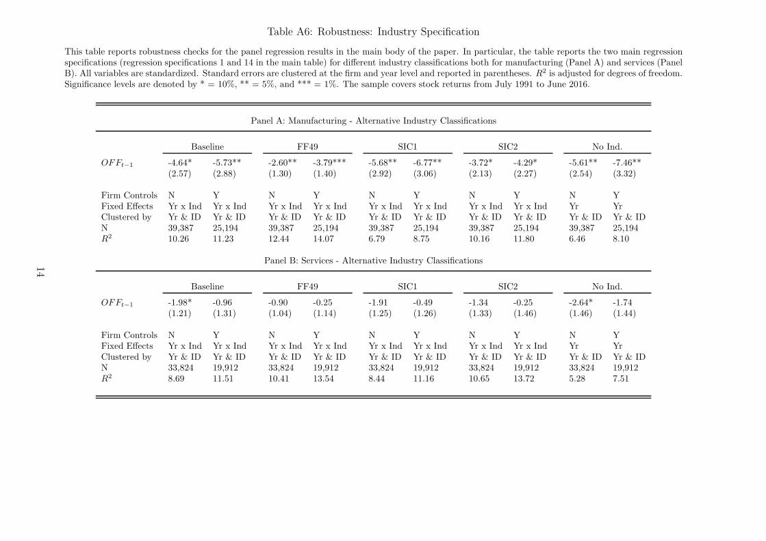
Table A6: Robustness: Industry Specification

This table reports robustness checks for the panel regression results in the main body of the paper. In particular, the table reports the two main regressionspecifications (regression specifications 1 and 14 in the main table) for different industry classifications both for manufacturing (Panel A) and services (PanelB). All variables are standardized. Standard errors are clustered at the firm and year level and reported in parentheses. R2 is adjusted for degrees of freedom.Significance levels are denoted by * = 10%, ** = 5%, and *** = 1%. The sample covers stock returns from July 1991 to June 2016.

Panel A: Manufacturing - Alternative Industry Classifications

Baseline FF49 SIC1 SIC2 No Ind.

OFFt−1 -4.64* -5.73** -2.60** -3.79*** -5.68** -6.77** -3.72* -4.29* -5.61** -7.46**(2.57) (2.88) (1.30) (1.40) (2.92) (3.06) (2.13) (2.27) (2.54) (3.32)

Firm Controls N Y N Y N Y N Y N YFixed Effects Yr x Ind Yr x Ind Yr x Ind Yr x Ind Yr x Ind Yr x Ind Yr x Ind Yr x Ind Yr YrClustered by Yr & ID Yr & ID Yr & ID Yr & ID Yr & ID Yr & ID Yr & ID Yr & ID Yr & ID Yr & IDN 39,387 25,194 39,387 25,194 39,387 25,194 39,387 25,194 39,387 25,194R2 10.26 11.23 12.44 14.07 6.79 8.75 10.16 11.80 6.46 8.10

Panel B: Services - Alternative Industry Classifications

Baseline FF49 SIC1 SIC2 No Ind.

OFFt−1 -1.98* -0.96 -0.90 -0.25 -1.91 -0.49 -1.34 -0.25 -2.64* -1.74(1.21) (1.31) (1.04) (1.14) (1.25) (1.26) (1.33) (1.46) (1.46) (1.44)

Firm Controls N Y N Y N Y N Y N YFixed Effects Yr x Ind Yr x Ind Yr x Ind Yr x Ind Yr x Ind Yr x Ind Yr x Ind Yr x Ind Yr YrClustered by Yr & ID Yr & ID Yr & ID Yr & ID Yr & ID Yr & ID Yr & ID Yr & ID Yr & ID Yr & IDN 33,824 19,912 33,824 19,912 33,824 19,912 33,824 19,912 33,824 19,912R2 8.69 11.51 10.41 13.54 8.44 11.16 10.65 13.72 5.28 7.51

14

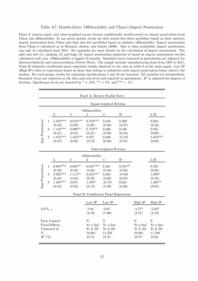
Table A7: Double-Sorts: Offshorability and China’s Import Penetration

Panel A reports equal- and value-weighted excess returns conditionally double-sorted on import penetration fromChina and offshorability. In any given month, stocks are first sorted into three portfolios based on their industryimport penetration from China and then into five portfolios based on industry offshorability. Import penetrationfrom China is calculated as in Bernard, Jensen, and Schott (2006). Due to data availability import penetrationcan only be calculated until 2011. See appendix for more details on the calculation of import penetration. Thesplit into low (1), medium (2) and high (3) import penetration industries is based on import penetration tercilescalculated each year. Offshorability is lagged 18 months. Standard errors reported in parentheses are adjusted forheteroscedasticity and autocorrelation (Newey-West). The sample includes manufacturing firms from 1991 to 2011.Panel B tabulates conditional panel regression results identical to the ones in table 9 of the main paper. Low IP(High IP) refers to regressions based on firms that belong to industries with import penetration below (above) themedian. For each group, results for regression specifications 1 and 10 are reported. All variables are standardized.Standard errors are clustered at the firm and year level and reported in parentheses. R2 is adjusted for degrees offreedom. Significance levels are denoted by * = 10%, ** = 5%, and *** = 1%.

Panel A: Return Double Sorts

Equal-weighted Returns

OffshorabilityL 2 3 4 H L-H

ImpPenetration 1 1.010*** 0.914*** 0.752*** 0.445 0.408 0.602

(0.33) (0.39) (0.30) (0.46) (0.27) (0.43)2 1.134*** 0.896** 0.778** 0.436 0.188 0.945

(0.41) (0.45) (0.37) (0.39) (0.44) (0.60)3 1.475*** 1.184*** 0.975 0.036 -0.135 1.610***

(0.47) (0.46) (0.73) (0.39) (0.47) (0.66)

Value-weighted Returns

OffshorabilityL 2 3 4 H L-H

ImpPenetration 1 0.805*** 0.662** 0.621*** 0.461 0.581** 0.224

(0.28) (0.30) (0.26) (0.43) (0.28) (0.39)2 0.925*** 1.111** 0.812*** 0.264 -0.168 1.093*

(0.35) (0.48) (0.32) (0.36) (0.48) (0.59)3 1.481*** 0.875 1.319* -0.175 0.021 1.460**

(0.42) (0.56) (0.74) (0.39) (0.46) (0.62)

Panel B: Conditional Panel Regressions

Low IP Low IP High IP High IP

OFFt−1 -1.84 -2.95 -4.77* -5.82*(2.58) (1.96) (2.57) (3.18)

Firm Control N Y N YFixed Effects Yr x Ind Yr x Ind Yr x Ind Yr x IndClustered by Yr & ID Yr & ID Yr & ID Yr & IDN 18,661 11,476 16,881 11,100R2 (%) 10.74 12.55 10.75 12.62

15

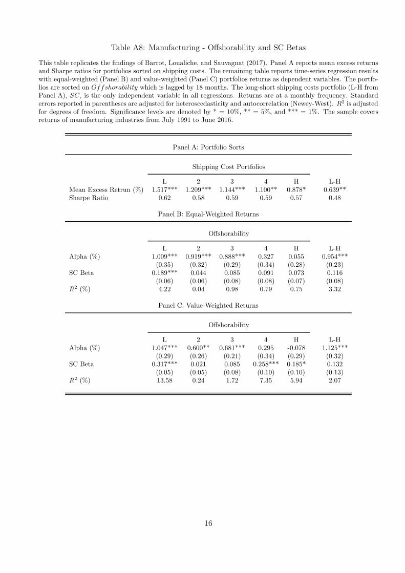
Table A8: Manufacturing - Offshorability and SC Betas

This table replicates the findings of Barrot, Loualiche, and Sauvagnat (2017). Panel A reports mean excess returnsand Sharpe ratios for portfolios sorted on shipping costs. The remaining table reports time-series regression resultswith equal-weighted (Panel B) and value-weighted (Panel C) portfolios returns as dependent variables. The portfo-lios are sorted on Offshorability which is lagged by 18 months. The long-short shipping costs portfolio (L-H fromPanel A), SC, is the only independent variable in all regressions. Returns are at a monthly frequency. Standarderrors reported in parentheses are adjusted for heteroscedasticity and autocorrelation (Newey-West). R2 is adjustedfor degrees of freedom. Significance levels are denoted by * = 10%, ** = 5%, and *** = 1%. The sample coversreturns of manufacturing industries from July 1991 to June 2016.

Panel A: Portfolio Sorts

Shipping Cost Portfolios

L 2 3 4 H L-HMean Excess Retrun (%) 1.517*** 1.209*** 1.144*** 1.100** 0.878* 0.639**Sharpe Ratio 0.62 0.58 0.59 0.59 0.57 0.48

Panel B: Equal-Weighted Returns

Offshorability

L 2 3 4 H L-HAlpha (%) 1.009*** 0.919*** 0.888*** 0.327 0.055 0.954***

(0.35) (0.32) (0.29) (0.34) (0.28) (0.23)SC Beta 0.189*** 0.044 0.085 0.091 0.073 0.116

(0.06) (0.06) (0.08) (0.08) (0.07) (0.08)R2 (%) 4.22 0.04 0.98 0.79 0.75 3.32

Panel C: Value-Weighted Returns

Offshorability

L 2 3 4 H L-HAlpha (%) 1.047*** 0.600** 0.681*** 0.295 -0.078 1.125***

(0.29) (0.26) (0.21) (0.34) (0.29) (0.32)SC Beta 0.317*** 0.021 0.085 0.258*** 0.185* 0.132

(0.05) (0.05) (0.08) (0.10) (0.10) (0.13)R2 (%) 13.58 0.24 1.72 7.35 5.94 2.07

16

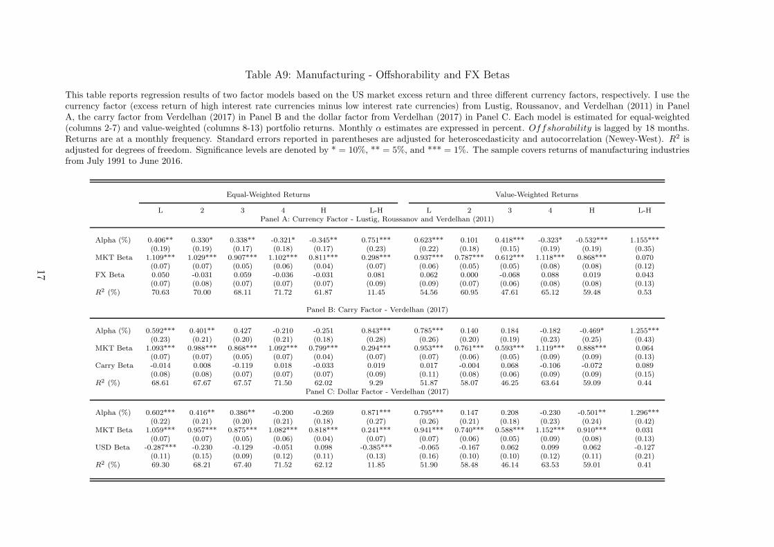
Table A9: Manufacturing - Offshorability and FX Betas

This table reports regression results of two factor models based on the US market excess return and three different currency factors, respectively. I use thecurrency factor (excess return of high interest rate currencies minus low interest rate currencies) from Lustig, Roussanov, and Verdelhan (2011) in PanelA, the carry factor from Verdelhan (2017) in Panel B and the dollar factor from Verdelhan (2017) in Panel C. Each model is estimated for equal-weighted(columns 2-7) and value-weighted (columns 8-13) portfolio returns. Monthly α estimates are expressed in percent. Offshorability is lagged by 18 months.Returns are at a monthly frequency. Standard errors reported in parentheses are adjusted for heteroscedasticity and autocorrelation (Newey-West). R2 isadjusted for degrees of freedom. Significance levels are denoted by * = 10%, ** = 5%, and *** = 1%. The sample covers returns of manufacturing industriesfrom July 1991 to June 2016.

Equal-Weighted Returns Value-Weighted Returns

L 2 3 4 H L-H L 2 3 4 H L-HPanel A: Currency Factor - Lustig, Roussanov and Verdelhan (2011)

Alpha (%) 0.406** 0.330* 0.338** -0.321* -0.345** 0.751*** 0.623*** 0.101 0.418*** -0.323* -0.532*** 1.155***(0.19) (0.19) (0.17) (0.18) (0.17) (0.23) (0.22) (0.18) (0.15) (0.19) (0.19) (0.35)

MKT Beta 1.109*** 1.029*** 0.907*** 1.102*** 0.811*** 0.298*** 0.937*** 0.787*** 0.612*** 1.118*** 0.868*** 0.070(0.07) (0.07) (0.05) (0.06) (0.04) (0.07) (0.06) (0.05) (0.05) (0.08) (0.08) (0.12)

FX Beta 0.050 -0.031 0.059 -0.036 -0.031 0.081 0.062 0.000 -0.068 0.088 0.019 0.043(0.07) (0.08) (0.07) (0.07) (0.07) (0.09) (0.09) (0.07) (0.06) (0.08) (0.08) (0.13)

R2 (%) 70.63 70.00 68.11 71.72 61.87 11.45 54.56 60.95 47.61 65.12 59.48 0.53

Panel B: Carry Factor - Verdelhan (2017)

Alpha (%) 0.592*** 0.401** 0.427 -0.210 -0.251 0.843*** 0.785*** 0.140 0.184 -0.182 -0.469* 1.255***(0.23) (0.21) (0.20) (0.21) (0.18) (0.28) (0.26) (0.20) (0.19) (0.23) (0.25) (0.43)

MKT Beta 1.093*** 0.988*** 0.868*** 1.092*** 0.799*** 0.294*** 0.953*** 0.761*** 0.593*** 1.119*** 0.888*** 0.064(0.07) (0.07) (0.05) (0.07) (0.04) (0.07) (0.07) (0.06) (0.05) (0.09) (0.09) (0.13)

Carry Beta -0.014 0.008 -0.119 0.018 -0.033 0.019 0.017 -0.004 0.068 -0.106 -0.072 0.089(0.08) (0.08) (0.07) (0.07) (0.07) (0.09) (0.11) (0.08) (0.06) (0.09) (0.09) (0.15)

R2 (%) 68.61 67.67 67.57 71.50 62.02 9.29 51.87 58.07 46.25 63.64 59.09 0.44Panel C: Dollar Factor - Verdelhan (2017)

Alpha (%) 0.602*** 0.416** 0.386** -0.200 -0.269 0.871*** 0.795*** 0.147 0.208 -0.230 -0.501** 1.296***(0.22) (0.21) (0.20) (0.21) (0.18) (0.27) (0.26) (0.21) (0.18) (0.23) (0.24) (0.42)

MKT Beta 1.059*** 0.957*** 0.875*** 1.082*** 0.818*** 0.241*** 0.941*** 0.740*** 0.588*** 1.152*** 0.910*** 0.031(0.07) (0.07) (0.05) (0.06) (0.04) (0.07) (0.07) (0.06) (0.05) (0.09) (0.08) (0.13)

USD Beta -0.287*** -0.230 -0.129 -0.051 0.098 -0.385*** -0.065 -0.167 0.062 0.099 0.062 -0.127(0.11) (0.15) (0.09) (0.12) (0.11) (0.13) (0.16) (0.10) (0.10) (0.12) (0.11) (0.21)

R2 (%) 69.30 68.21 67.40 71.52 62.12 11.85 51.90 58.48 46.14 63.53 59.01 0.41

17

Table A10: Low-wage Countries

This table lists the low-wage countries. I follow Bernard, Jensen, and Schott (2006) and define a country as low-wagein year t if its per capita GDP is less than 5% of U.S. per capita GDP.

Afghanistan China India PakistanAlbania Comoros Kenya RwandaAngola Congo Lao PDR SamoaArmenia Equitorial Guinea Lesotho Sao TomeAzerbaijan Eritrea Madagascar Sierra LeoneBangladesh Ethiopia Malawi SomaliaBenin Gambia Maldives Sri LankaBhutan Georgia Mali St. VincentBurkina Faso Ghana Mauritania SudanBurundi Guinea Moldova TogoCambodia Guinea-Bissau Mozambique UgandaCentral African Rep Guyana Nepal VietnamChad Haiti Niger Yemen

18

References

Acemoglu, D., and D. H. Autor (2011): “Skills, tasks and technologies: Implications for employmentand earnings,” Handbook of Labor Economics, 4, 1043–1171.

Acemoglu, D., D. H. Autor, D. Dorn, G. H. Hanson, and B. Price (2016): “Import Competitionand the Great U.S. Employment Sag of the 2000s,” jole, 34, S141–S198.

Amiti, M., and S.-J. Wei (2009): “Service Offshoring and Productivity: Evidence from the US,” The

World Economy, 32, 203–220.

Autor, D. H., D. Dorn, and G. H. Hanson (2013): “The Cina Syndrome: Local Labor MarketEffects of Import Competition in the United States,” American Economic Review, 103, 2121–2168.

(2016): “The China Shock: Learning from Labor Market Adjustment to Large Changes inTrade,” Annual Review of Economics, forthcoming.

Barrot, J.-N., E. Loualiche, and J. Sauvagnat (2017): “The Globalization Risk Premium,” Work-ing Paper.

Belo, F., X. Lin, and S. Bazdresch (2014): “Labor hiring, investment and stock return predictabilityin the cross section,” Journal of Political Economy, 122, 129–177.

Bernard, A. B., J. B. Jensen, and P. K. Schott (2006): “Survival of the Best Fit: Low WageCompetition and the (Uneven) Growth of Manufacturing Plants,” Journal of Interantional Economics,68, 219–237.

Blinder, A. S. (2009): “How Many U.S. Jobs Might Be Offshorable,” World Economics, 10, 41–78.

Dasgupta, S., T. H. Noe, and Z. Wang (2011): “Where Did All the Dollars Go? The Effect of CashFlows on Capital and Asset Structure,” Journal of Quantitative Analysis, 46, 1259–1294.

Donangelo, A. (2014): “Labor Mobility: Implications for Asset Pricing,” Journal of Finance, 68,1321–1346.

Fama, E. F., and K. R. French (1988): “Permanent and Temporary Components of Stock Prices,”Journal of Political Economy, 96, 246–273.

(1992): “The cross-section of expected stock returns,” Journal of Finance, 47, 427–465.

(1993): “Common risk factors in the returns on stocks and bonds,” Journal of Financial Eco-

nomics, 33, 3–56.

(1997): “Industry costs of equity,” Journal of Financial Economics, 43, 153–193.

(2015): “A five-factor asset pricing model,” Journal of Financial Economics, 116, 1–22.

Fan, J. P., S. Titman, and G. Twite (2012): “An international comparison of capital structure anddebt maturity choices,” Journal of Quantitative Analysis, 47, 23–56.

Fillat, J. L., and S. Garetto (2015): “Risk, Returns, and Multinational Production,” Quarterly

Journal of Economics, 130, 2027–2073.

Firpo, S., N. Fortin, and T. Lemieux (2013): “Occupational Tasks and Changes in the Wage Struc-ture,” Working Paper.

19

Jensen, B. J. (2011): Global Trade in Services: Fear, Facts, and Offshoring. Peterson Institute ForInternational Economics, 1 edn.

Lustig, H., N. Roussanov, and A. Verdelhan (2011): “Common Risk Factors in Currency Markets,”Review of Financial Studies, 24, 3731–3777.

Malmendier, U., and G. Tate (2005): “CEO overconfidence and corporate investment,” Journal of

Finance, 65, 2661–2700.

Minton, B. A., and C. Schrand (1999): “The impact of cash flow volatility on discretionary investmentand the cost of debt and equity financing,” Journal of Financial Economics, 54, 423–460.

Novy-Marx, R. (2011): “Operating leverage,” Review of Finance, 15, 103–134.

Ochoa, M. J. (2013): “Volatility, Labor Heterogeneity and Asset Prices,” Working Paper.

Patton, A. J., and A. Timmermann (2010): “Monotonicity in asset returns: New tests with appli-cations to the term structure, the CAPM, and portfolio sorts,” Journal of Financial Economics, 98,605–625.

Verdelhan, A. (2017): “The Share of Sytematic Variation in Bilateral Exchange Rates,” Journal of

Finance, forhcoming.

Zhang, M. B. (2016): “Labor-Technology Substitution: Implications for Asset Pricing,” Working Paper.

20