Friction Stir Welding Manufacturing Advancement by On-Line

Louisiana State UniversityLSU Digital Commons

LSU Doctoral Dissertations Graduate School

11-7-2017

Friction Stir Welding Manufacturing Advancementby On-Line High Temperature Phased ArrayUltrasonic Testing and Correlation of ProcessParameters to Joint QualityDaniel James HuggettLouisiana State University and Agricultural and Mechanical College, [email protected]

Follow this and additional works at: https://digitalcommons.lsu.edu/gradschool_dissertations

Part of the Manufacturing Commons, and the Metallurgy Commons

This Dissertation is brought to you for free and open access by the Graduate School at LSU Digital Commons. It has been accepted for inclusion inLSU Doctoral Dissertations by an authorized graduate school editor of LSU Digital Commons. For more information, please [email protected].

Recommended CitationHuggett, Daniel James, "Friction Stir Welding Manufacturing Advancement by On-Line High Temperature Phased Array UltrasonicTesting and Correlation of Process Parameters to Joint Quality" (2017). LSU Doctoral Dissertations. 4139.https://digitalcommons.lsu.edu/gradschool_dissertations/4139

https://digitalcommons.lsu.edu?utm_source=digitalcommons.lsu.edu%2Fgradschool_dissertations%2F4139&utm_medium=PDF&utm_campaign=PDFCoverPages

https://digitalcommons.lsu.edu/gradschool_dissertations?utm_source=digitalcommons.lsu.edu%2Fgradschool_dissertations%2F4139&utm_medium=PDF&utm_campaign=PDFCoverPages

https://digitalcommons.lsu.edu/gradschool?utm_source=digitalcommons.lsu.edu%2Fgradschool_dissertations%2F4139&utm_medium=PDF&utm_campaign=PDFCoverPages

https://digitalcommons.lsu.edu/gradschool_dissertations?utm_source=digitalcommons.lsu.edu%2Fgradschool_dissertations%2F4139&utm_medium=PDF&utm_campaign=PDFCoverPages

http://network.bepress.com/hgg/discipline/301?utm_source=digitalcommons.lsu.edu%2Fgradschool_dissertations%2F4139&utm_medium=PDF&utm_campaign=PDFCoverPages

http://network.bepress.com/hgg/discipline/288?utm_source=digitalcommons.lsu.edu%2Fgradschool_dissertations%2F4139&utm_medium=PDF&utm_campaign=PDFCoverPages

https://digitalcommons.lsu.edu/gradschool_dissertations/4139?utm_source=digitalcommons.lsu.edu%2Fgradschool_dissertations%2F4139&utm_medium=PDF&utm_campaign=PDFCoverPages

mailto:[email protected]

FRICTION STIR WELDING MANUFACTURING ADVANCEMENT BY ON-

LINE HIGH TEMPERATURE PHASED ARRAY ULTRASONIC TESTING

AND CORRELATION OF PROCESS PARAMETERS TO JOINT QUALITY

A Dissertation

Submitted to the Graduate Faculty of the

Louisiana State University and

Agricultural and Mechanical College

in partial fulfillment of the

requirements for the degree of

Doctor of Philosophy

in

The Department of Mechanical Engineering

by

Daniel James Huggett

B.S., Southeastern Louisiana State University, 2012

December 2017

ii

To my family, parents (Kathryn and James Huggett), siblings (Karyn and Laura Huggett), and

wife (Danielle Huggett) for your steadfast support, sacrifices, and unconditional love. Without

you, this achievement would not be possible.

iii

ACKNOWLEDGEMENTS

Articulation of an appropriate expression of gratitude is difficult, as words cannot convey

the appreciation I have for the people who provided moral and technical support through my

academic career. I only hope that this acknowledgement can somewhat indicate fully the gratitude

I have for those who helped me.

Firstly, I would like to acknowledge my advisor, Dr. Muhammad Wahab. I would not have

been able to experience the opportunities this program has provided without your encouragement

to work on my PhD. Your unconditional support and guidance was truly incredible, and I will

utterly miss our discussions. Secondly, I would like to direct attention to Dr. Warren Liao and Dr.

Ayman Okeil, panel professors and mentors. Your constant help, guidance, and critique through

my graduate career have propelled my capabilities as a student and engineer.

I am grateful to the employees at the Michoud Assembly Facility (MAF) and National

Center for Advanced Manufacturing (NCAM). I would like to personally thank John Alt for his

guidance, training, and technical insight. My experiences with you provided real world skills that

I would never have learned in any classroom. The author would like to thank Dr. Michael Eller,

whose technical guidance and expertise are unparalleled. My time spent in your class solidified

my understanding of the friction stir welding technique which I will be able to call upon in my

future career.

To Dr. Arthur Nunes, Jr., NASA technical advisor through my doctoral program, who

provided life changing advice on engineering and technical writing skills. Your vast knowledge of

welding, engineering, and literature are truly remarkable. I have learned much through our

conversations over the years. Your lessons have had a profound impact in my development as an

engineer.

iv

Recognition is in order to the National Aeronautics and Space Administration. I have had

two summer internships with NASA at the John C. Stennis Space Center and Marshall Space Flight

Center. I have also participated in the NASA Pathways Program, where I worked at the Kennedy

Space Center. NASA’s opportunities to instruct students to develop into aspiring engineers is

greatly appreciated. My mentors in those programs were exceptional, including Dr. Harry Ryan,

Dr. David Coote, Dr. Alok Majumdar, Dr. Andre LeClair, Patrick Maloney, and the members of

the KSC Engineering Analysis Branch. Moreover, thanks to NASA for funding my research and

allowing me to utilize MAF and NCAM facilities.

I am grateful to my grandfathers, each who have a deep history with Louisiana State

University. Dr. Alfred J. Cox, Jr., graduate of LSU in Chemistry, a.k.a. Papa, is one of the most

influential persons in my life. Growing up, I tried to emulate him. His perseverance, wisdom, and

never ending passion to understand mechanical systems influenced me greatly. Dr. Richard

Huggett, retired professor of physics from LSU, a.k.a. Papa Huggett, was an inspiration to me

growing up. I often recall our astronomy nights where we would use his telescope to look at the

moon and stars, which began my fascination with the aerospace discipline. I would also like to

acknowledge Michael Cox, a.k.a Uncle Mike, who was a role model in my life. Thank you for

your guidance and support throughout the years.

Lastly, I would like to thank my colleagues and lab mates. These include Dr. Mohammad

Dewan, Dr. Jasem Ahmet, Dr. Saad Aziz, Dr. Jizhou Fan, Joshua Palmer, and Luke Bilich. I feel

we have created a life-long friendship, and your help and support through my graduate program is

greatly appreciated. I will miss our lunch breaks and stimulating discussions.

ii

TABLE OF CONTENTS

ACKNOWLEDGEMENTS ........................................................................................................... iii

LIST OF TABLES .......................................................................................................................... v

LIST OF FIGURES ...................................................................................................................... vii

NOMENCLATURE .................................................................................................................... xiv

ABSTRACT ............................................................................................................................... xviii

CHAPTER 1 : INTRODUCTION .................................................................................................. 1

CHAPTER 2 : THE TECHNIQUE OF FRICTION STIR WELDING .......................................... 4

2.1. Overview of FSW in Industry .............................................................................................. 4 2.2. Overview of the FSW Process ............................................................................................. 6 2.3. FSW Mechanical Properties ................................................................................................ 8

2.4. FSW Literature Trends and Dissertation Work Significance ............................................ 12

CHAPTER 3 : NON-DESTRUCTIVE TESTING AND EVALUATION .................................. 14 3.1. Introduction ........................................................................................................................ 14 3.2. Ultrasonic Testing (UT) ..................................................................................................... 15

3.3. Conventional Ultrasonic Testing ....................................................................................... 21

3.4. Time of Flight Diffraction (TOFD) ................................................................................... 22

3.5. Phased Array Ultrasonic Testing (PAUT) ......................................................................... 23 3.6. Defect Sizing using PAUT................................................................................................. 28

3.7. Radiographic Testing (RT) ................................................................................................ 31

CHAPTER 4 : EXPERIMENTAL FACILITIES, TOOLING, AND WELDING

METHODOLOGY .............................................................................................. 33 4.1. Facilities ............................................................................................................................. 33

4.2. FSW Tooling ...................................................................................................................... 39 4.3. FS Weld Experimental Methodology ................................................................................ 41

CHAPTER 5 : FSW AA-2219 LITERATURE REVIEW ............................................................ 43

5.1. Introduction ........................................................................................................................ 43 5.2. Literature Review on FSW of AA-2219 ............................................................................ 44

CHAPTER 6 : FSW DEFECTS AND QUALITY CLASSIFICATION ...................................... 65 6.1. Introduction ........................................................................................................................ 65 6.2. FSW Process Parameters ................................................................................................... 65 6.3. Microstructure of FSW Joints ............................................................................................ 66 6.4. Weld Defect Classification ................................................................................................ 70 6.5. Tensile Properties of FS Welds.......................................................................................... 77 6.6. Fracture Surface Analysis .................................................................................................. 79

iii

6.7. Micro-Hardness of FS Welds............................................................................................. 83 6.8. Summary ............................................................................................................................ 84

CHAPTER 7 : DEVELOPMENT OF A NEW PROCESS PARAMETER METHODOLOGY

AND EMPIRICAL FORCE INDEX TO DETERMINE WELD QUALITY ...... 85 7.1. Introduction ........................................................................................................................ 85 7.2. Development of the Pin Speed Ratio ................................................................................. 86 7.3. Process Parameter Window ............................................................................................... 93 7.4. Empirical Force Index ........................................................................................................ 97

7.5. Conclusions ...................................................................................................................... 100

CHAPTER 8 : PREDICTION OF FRICTION STIR WELD QUALITY WITH AND

WITHOUT SIGNAL FEATURES ..................................................................... 102 8.1. Introduction ...................................................................................................................... 102 8.2. FSW Experimentation, Weld Classes, and Signal Feature Extraction ............................ 105

8.3. Classification Methodology ............................................................................................. 113 8.4. Results and Discussion .................................................................................................... 116

8.5. Conclusions ...................................................................................................................... 125

CHAPTER 9 : DEFECT SUPPRESSION MODEL FOR FIXED PIN FSW ............................ 126

9.1. Introduction ...................................................................................................................... 126 9.2. Procedure ......................................................................................................................... 129

9.3. Results .............................................................................................................................. 132 9.4. Analysis of Results .......................................................................................................... 133

9.5. Conclusion ....................................................................................................................... 142

CHAPTER 10 : DEVELOPMENT OF HIGH TEMPERATURE ULTRASONIC

TESTING FOR FSW ........................................................................................ 143 10.1. Introduction .................................................................................................................... 143

10.2. PAUT and FSW Experiments ........................................................................................ 146 10.3. PAUT vs. X-Ray Radiography for Post-Weld Inspection ............................................. 149

10.4. On-line PAUT ................................................................................................................ 157 10.5. Conclusions .................................................................................................................... 167

CHAPTER 11 : ON-LINE HIGH TEMPERATURE PHASED ARRAY ULTRASONIC

INSPECTION OF FIXED PIN FRICTION STIR WELDS AND ITS

IMPACT ON WELD QUALITY ..................................................................... 169

11.1. Introduction .................................................................................................................... 169 11.2. Experimental Conditions ............................................................................................... 171 11.3. Design of Two On-Line HT-PAUT FSW Systems ....................................................... 172

11.4. Defect Observations and HT-PAUT Impact on Microstructure .................................... 177 11.5. Conclusion ..................................................................................................................... 185

CHAPTER 12 : CONCLUSION ................................................................................................ 187 12.1. Overview ........................................................................................................................ 187 12.2. Synopsis of Work Completed ........................................................................................ 187

iv

12.3. Discussion of Future FSW Work ................................................................................... 189

REFERENCES…………………………………………………………………………………191

APPENDIX : Supplemental Data ............................................................................................... 212

VITA ........................................................................................................................................... 219

v

LIST OF TABLES

Table 2-1: Weld Strength Summary from Various FSW Studies ................................................. 12

Table 3-1 : Common NDT Techniques and their applications ..................................................... 16

Table 3-2 : Interpretation of Time-Of-Flight-Diffraction (TOFD) ultrasonic images .................. 24

Table 3-3 : Comparison of Defect Sizing of PAUT ..................................................................... 30

Table 5-1 : Process Development and Mechanical Properties...................................................... 47

Table 5-2 : Residual Stress and Post-Weld Heat Treatment ......................................................... 52

Table 5-3 : Corrosion of AA-2219 Welds .................................................................................... 54

Table 5-4 : FSW of Dissimilar Materials Including AA-2219 ..................................................... 55

Table 5-5 : FSW vs. Fusion Welding of AA-2219 ....................................................................... 56

Table 5-6 : Non-Conventional FSW of AA-2219 and Special Studies ........................................ 57

Table 7-1 : Verification of the effect of speed ratio (R) ............................................................... 93

Table 7-2: New weld schedules along with weld quality for the validation of developed

of empirical force index (EFI) in weld classification. (NW – Nominal Weld,

CW – Cold Weld) ..................................................................................................... 100

Table 8-1: Data-driven modelling works that pertain to FSW aiming to predict weld

quality* ..................................................................................................................... 103

Table 8-2: Weld quality values for EFI with associated averages .............................................. 108

Table 8-3: Classification error rates for weld quality utilizing KNN and FKNN with

all features. ................................................................................................................ 116

Table 8-4: Classification error rates of weld Quality for KNN and FKNN coupled

with Metaheuristic ABC ........................................................................................... 117

Table 8-5: Weld schedules which promote inacurrate classification due to having a

combination of process parameters which lie on the boundaries of hot/

nominal and cold/nominal weld quality (3 – Hot Weld, 8 – Cold Weld) ................. 120

Table 8-6: Classification error rates for weld quality utilizing KNN and FKNN with

all features without boundary data sets ..................................................................... 121

vi


with Metaheuristic ABC without boundary data sets ............................................... 121


with Metaheuristic ABC employing additional features obtained from

weld signals ............................................................................................................... 124

Table 9-1: FSW weld schedules conducted with I-Stir UWS #2 with defects (DF

- defect free, TR - Trenching defect, WH - wormhole, IP – Incomplete

Penetration, UF/F - Underfill/Flash defect, Internal voids - V). .............................. 126

Table 9-2: FSW Weld Schedules conducted on I-Stir PDS Welder with Associated

Characteristics (DF - defect free, TR - Trenching defect, WH - wormhole,

IP –Incomplete Penetration, UF/F - Underfill/Flash defect, Internal voids - V). ...... 127

Table 9-3: Parameters used in weld temperature estimates. ....................................................... 138

Table 10-1: Various IP defects with defect height from root of weld ........................................ 155

Table 10-2 : Accuracy and Precision of PAUT HT transducer/wedge unit at ambient

temperature ............................................................................................................ 161

Table 10-3 : Comparison of two SDHs at increasing temperatures ............................................ 161

Table 10-4 : FSW Process Parameters for Online PAUT Demos .............................................. 164

Table 11-1: Weld schedules conducted with both OLSSs to review performance of

analyzing defects ..................................................................................................... 178

Table 11-2: FSW weld schedules conducted with I-Stir PDS with associated defect

identification (DF - defect free, IP – Incomplete Penetration, Pl. Force

– Plunge Force, Sch. – Schedule, Tough. – Toughness, TR – Trenching

defect) .................................................................................................................... 181

Table 11-3: Advantages and Disadvantages of each OLSS developed in the study .................. 186

vii

LIST OF FIGURES

Figure 2-1: Friction stir welding pin tool types .............................................................................. 7

Figure 2-2: FSW AS and RS orientation per (A) clockwise rotation and (B) counter

clockwise rotation ........................................................................................................ 8

Figure 2-3: Macrograph of FS weld cross-section illustrating the four distinct micro

structure zones ............................................................................................................. 9

Figure 2-4: Heat-treatable alloy FS weld hardness profile ........................................................... 11

Figure 2-5: Non-heat-treatable alloy FS weld hardness profile .................................................... 11

Figure 3-1 : Radiated fields from an ultrasonic transducer: near-field and far-field .................... 19

Figure 3-2 : Beam-spread and beam-divergence during ultrasonic testing .................................. 19

Figure 3-3 : Schematic of conventional UT, TOFD, and PAUT created with ultrasonic

simulation software (ESBeam Tool) ......................................................................... 20

Figure 3-4 : Phased array ultrasonic scan pattern and different scan views ................................. 20

Figure 3-5 : Schematic of ultrasonic method to calculate defect location .................................... 21

Figure 3-6 : Typical A-scan signal indicating received signal voltage vs. time. .......................... 22

Figure 3-7 : Schematic of TOFD scanning process and typical TOFD A and B scan

views showing different echoes ................................................................................ 23

Figure 3-8 : A typical probe and wedge configuration with illustration of wave

propagation inside a FS welded specimen ................................................................ 26

Figure 3-9 : PAUT A, S, and C-scan view acquired using Olympus Omniscan

MX2.0 data acquisition unit ...................................................................................... 27

Figure 3-10 : Effect of A-scan amplitude and color drop on defect size estimation .................... 28

Figure 3-11 : Effect of index offset and color drop on defect size estimation (fixed

gain value) ............................................................................................................... 29

Figure 3-12 : Variations of A-scan amplitude with index offset to illustrate the effect

of TCG calibration .................................................................................................. 29

Figure 3-13 : Aluminum alloy plate with seven varying hole sizes with associated C

-scan and eco-dynamic A-Scan images. ................................................................. 30

viii

Figure 3-14 : Schematic of Basic Set-up for film radiography ..................................................... 31

Figure 4-1 : Weld platforms employed throughout the experimental program

(Courtesy NCAM) .................................................................................................... 34

Figure 4-2: MTS-810 uniaxial tensile test set-up including hydraulic unit wedge

grips FSW tensile specimen and MTS extensometer ................................................. 36

Figure 4-3 : FUTURE-TECH Rockwell Hardness Tester ............................................................ 36

Figure 4-4: MetaServe 250 Polisher/Grinder employed through the doctoral work .................... 36

Figure 4-5 : Metallurgical microscope utilized for microstructural analysis ................................ 37

Figure 4-6 : Band Saw utilized for cutting FS welded tensile and macro coupons ...................... 37

Figure 4-7: OMNIScan MX2 Data acquisition system employed for PAUT

inspection through the entirety of this work .............................................................. 38

Figure 4-8: Select PAUT transducers and wedges employed through the work. Going

from left to right: Olympus Weld Series 5L32-A31 transducer ................................ 38

Figure 4-9: Liquid dye penetrant testing equipment employed for weld surface defect

examination ................................................................................................................ 38

Figure 4-10 : JSM -6610 LV SEM located at the SIF on LSU campus........................................ 39

Figure 4-11: Pin Tool employed during FSW experiments (top) and interchangeable

threaded pin (bottom) ............................................................................................... 40

Figure 4-12: FSW fixture employed during weld operations ....................................................... 40

Figure 6-1 : Line diagram showing factors that affect the quality of a FSW joint ....................... 66

Figure 6-2: Cross-sectional view of FS welded joint. A FSW joint is composed of SZ,

TMAZ, HAZ, and base metal .................................................................................... 67

Figure 6-3: Optical micrographs of defect-free FS welded AA-2219 joint. Micrographs

are taken at different locations showing variations in microstructure ....................... 67

Figure 6-4: Midsectional plan-view of macro- and microstructure created by the FSW pin

, tool spindle rotating clockwise at 400 RPM with feedrate of 4 IPM....................... 68

Figure 6-5: Top surface plan-view of macro- and microstructure created by the FSW tool

shoulder and pin, tool spindle rotating clockwise at 400 RPM, feedrate. ................. 69

ix

Figure 6-6: SEM micrographs of a defect-free FS welded AA-2219-T87 joint. Micro

graphs are taken at different locations in the weld showing variations ..................... 69

Figure 6-7: Electron backscatter diffraction (EBSD) images of FS welded AA-2xxx

(Image Courtesy: Oxford-EBSD) ............................................................................... 70

Figure 6-8 : General classification of welds utilized in this work ................................................ 71

Figure 6-9: Cold weld showing TR, WH, and IP defects ............................................................. 72

Figure 6-10: Hot-weld showing IV (left) and UF (right) .............................................................. 72

Figure 6-11 : Schematic of FS welded panel with schedule and transition zones.

Transition zones are transient regions. PTZ is plunge transition ............................ 74

Figure 6-12 : Force profiles vs. time (signal data acquisition rate 60 Hz). Schedule 1

[200 RPM -152.4 mm/min - 33.36 kN]; Schedule 2 [450 RPM - 152.4 ................. 75

Figure 6-13 : Optical micrographs of cross-section and fracture specimen of a defect free

and defective specimen with WH and IP. SEM images illustrate .......................... 76

Figure 6-14: Stress-strain plots of base and FS welded AA2219-T87 specimens (base

, nominal, hot, and cold welds) ................................................................................ 78

Figure 6-15: Typical SEM micrographs showing microstructure in the weld nugget

(WN) of (a) nominal weld (NW), (b) hot weld (HW), and (c) cold ........................ 78

Figure 6-16: Effect of different weld defects on tensile properties (NW: nominal weld;

HW: hot weld; CW-IP: cold weld with incomplete penetration .............................. 79

Figure 6-17: Nominal weld showing no defect. A 45° maximum shear fracture is on

retreating side of tool outside the weld nugget in heat-affected .............................. 80

Figure 6-18: Hot weld showing an IV. Fracture is on the AS of the tool inside the SZ.

Fracture surface exhibits equiaxed ductile fracture dimples, smaller ...................... 81

Figure 6-19: Cold weld showing internal cavity. Fracture is on the AS of tool inside the

weld nugget. Fracture surface exhibits ductile fracture dimples ............................. 82

Figure 6-20: Cold weld showing TR defect at weld crown and IP at weld root. Fracture

is on AS of tool inside the weld nugget. Fracture surface exhibits .......................... 83

Figure 6-21: (a) Cross sectional view and (b) Micro-hardness profile of FS- welded AA

2219-T87 joint .................................................................................................... 84

x

Figure 7-1: Experimental ultimate tensile strength (UTS) values are plotted against (a)

energy input, (b) Pseudo heat index, and c)Alternative heat index ........................... 88

Figure 7-2 : Effect of plunge force on tensile strength and toughness at constant rotation .......... 90

Figure 7-3: Effect of speed ratio (𝑅) on (a) UTS and (b) Toughness at constant plunge

force (Fz) .................................................................................................................... 91

Figure 7-4: Effect of plunge force (Fz) on (a) ultimate tensile strength (UTS) and (b) Toughness

at two different speed ratio (R) ..................................................................................................... 92

Figure 7-5: FSW process parameters for hot, nominal, and cold welds group together into

fields with distinct boundaries ................................................................................... 95

Figure 7-6 : Internal Void (V) defect macrograph (top left) and micrograph (top right) with

associated PAUT A-Scan (bottom left) and S-Scan (bottom right) .......................... 97

Figure 7-7: Plunge force vs. speed ratio plotted to obtain empirical correlation among three

weld process parameters for nominal weld ................................................................ 99

Figure 7-8: Variations of tensile properties with empirical force index (EFI): (left)

Toughness vs. EFI, and (right) Ultimate tensile strength vs. EFI. ............................ 99

Figure 8-1: A) FSW configuration employed in this work during operation illustrating

the three process parameters that compose a weld schedule; B) ............................. 106

Figure 8-2: Plan surfaces (left) and transverse sections (right) of a Nominal, Hot, and

Cold weld specimen ................................................................................................. 107

Figure 8-3: Process parameter window illustrating weld quality classes and the boundaries

between hot and nominal as well as cold and nominal weld conditions ................. 109

Figure 8-4: Weld quality classes based upon EFI, UTS, and Toughness ................................... 110

Figure 8-5: FSW signal data illustrating weld signal data of X-, Y-, and plunge forces

indicating the change in steady-state conditions when a TR defect forms .............. 111

Figure 8-6: Convergence profile of KNN + ABC where population size=10 with 10-

Fold CV .................................................................................................................... 118

Figure 9-1: Left: Top views of friction stir welds: Nominal weld shows well defined ripple

pattern. Hot weld shows flash on retreating side, irregular (flash-related) .............. 129

Figure 9-2: FSW machines used to perform welds: (A) I-Stir PDS, (B) I-STIR UWS #2.

FSW in progress between clamps and steel bars holding panel against .................. 130

xi

Figure 9-3: Above: Forces vs. time during FSW weld process example [Schedule 1: 200

RPM, 152.4 mm/min, 33.36 kN followed by Schedule 2: 450 RPM ...................... 131

Figure 9-4: Schematic representation of isotherms bounding area of parameter

combinations yielding sound friction stir welds ...................................................... 133

Figure 9-5: Macrostructure at transverse section of FS weld showing trace of shear

surface. Above is shown schematically the shear surface and the plug. .................. 135

Figure 9-6: Schematic model for heat balance used to approximate weld temperatures ............ 136

Figure 9-7: Map of cold, hot, and nominal (no defects) weld conditions in coordinates

of plunge force and weld temperature indicator Rω/V. The nominal ...................... 140

Figure 10-1 : A typical probe and wedge configuration with illustration of wave

propagation ........................................................................................................... 147

Figure 10-2 : (a) PAUT S-scan Image displaying the effect of SDH at larger depth,

with associated schematic of first and second legs with SDH defect (b) ............. 148

Figure 10-3 : Illustration of PAUT system with various legs indicating where FSW

defects may occur. ................................................................................................ 149

Figure 10-4 : Optical image of cross-section, enlarged defect image, PAUT A-Scan

and S-Scan image (second leg) of FS welded panel with surface ........................ 150

Figure 10-5 : Radiographic, PAUT B-Scan, and PAUT C-Scan images.................................... 151

Figure 10-6 : Optical image of cross-section, enlarged defect image, PAUT A-Scan and

S-Scan image of FS welded panel with wormhole defect .................................... 151

Figure 10-7 : Radiographic, PAUT B-Scan, and PAUT C-Scan images of a FS welded

panel with wormhole defect .................................................................................. 151

Figure 10-8 : Optical image of cross-section, enlarged defect image, PAUT A-Scan and

S-Scan image of FS welded panel with SC defect (Observed by Second Leg) .... 152

Figure 10-9 : Radiographic, PAUT B-Scan, and PAUT C-Scan images of a FS welded

panel with SC defect ............................................................................................. 152

Figure 10-10 : Optical image of cross-section, enlarged defect image, PAUT A-Scan

and S-Scan image of FS welded panel with internal void .................................. 153

Figure 10-11 : Radiographic image, PAUT B-Scan image, and C-Scan image of FSW

panel with internal void ...................................................................................... 153

xii

Figure 10-12 : Optical image (left) of IP defect of length 480 µm and associated S-scan

image (right) of IP defect .................................................................................... 156

Figure 10-13 : A) Optical micrograph of IP defect, B) Optical image of tensile tested

specimen indicating fracture origination; C) SEM image indicating un-

bonded area ........................................................................................................ 156

Figure 10-14 : Custom PAUT HT wedge/transducer unit .......................................................... 159

Figure 10-15 : Illustration of HT PAUT for SDH AA-2219 specimen of 8.13 mm

thickness .............................................................................................................. 159

Figure 10-16 : Comparison of A- and S-scan images of 1.19 mm diameter SDH at a depth

of 6.3 mm. Case A) conducted at room temperature, and case B) ..................... 162

Figure 10-17 : Effect of temperature on defect measurement for HT PAUT system for

SDH of diameter 0.79 mm (top) and 1.19 mm (bottom) .................................... 162

Figure 10-18 : PAUT ambient temperature wedge (left), custom HT wedge, and

commercial HT wedge ........................................................................................ 163

Figure 10-19: Image of FSW fixture employed in this study ..................................................... 164

Figure 10-20 : Custom PAUT HT wedge/transducer unit scanning during FSW ...................... 165

Figure 10-21 : PAUT S-scan images of HT wedge/transducer unit signals: a) un-welded

seam, b) nominal welded seam, c) TR defect welded seam ............................... 166

Figure 10-22 : PAUT illustration of multiple legs scanning a FS weld with a TR defect on

AS ....................................................................................................................... 166

Figure 11-1: A) Fixed pin tool and B) I-Stir PDS machine employed in this study,

and C) the FSW process during experimentation at the NASA Michoud ............. 172

Figure 11-2: OLSS-1 design illustrating the 4 subassemblies of the system (left) and the

OLSS-1 attached to the PDS FS welder at the NASA Michoud ........................... 175

Figure 11-3: Variation of FSW fixture employed during experimentation: A) Nominal

FSW fixture configuration, B) FSW fixture with chill bar offset .......................... 176

Figure 11-4: OLSS-2 design illustrating the 4 subassemblies of the system. The hole

cut-outs in the magnetic fastening and HT-PAUT transducer ............................... 177

Figure 11-5: Process parameter map of weld schedules classified as hot, cold, and

nominal plotted with plunge force vs. PSR. The hot class of welds ...................... 178

xiii

Figure 11-6: OLSS-1 in operation during FSW discovering a TR defect (Top) with

associated PAUT A- (Bottom Left) and S-scan (Bottom Right) images ............... 179

Figure 11-7: OLSS-2 in operation during FSW discovering a WH defect (Top) with

associated PAUT A- (Bottom Left) and S-scan (Bottom Right) images ............... 180

Figure 11-8: Transverse cross-sections of FSW joints comparing 4 weld schedules with

nominal, OLSS-1, and OLSS-2 fixture conditions. In each transverse. ............... 183

Figure 11-9: Select fracture specimens from schedule #1 from OLSS-1 weld configuration .... 183

Figure 11-10: Transverse section of schedule #4 with OLSS-1 configuration where the

variation in fixture conditions caused indentation at the AS of the panel .......... 184

xiv

NOMENCLATURE

AA Aluminum alloy

ABC Artificial Bee Colony

ACO Ant Colony Optimization

AE Acoustic Emissions

AHI Alternative heat index

ANFIS Adaptive neuro-fuzzy inference system

ANSI American National Standards Institute

AS Advancing side

ASNT American Society of Non-destructive Testing

ASTM American Society for Testing and Materials

BOK Body of Knowledge

CCE Connected Component Extraction

CCW Counter Clock Wise

CDRX Continuous Dynamically Recrystallized Grains

CW Cold weld

CR Computed Radiography

CT Computed Tomography

DDRX Discontinuous Dynamically Recrystallized Grains

DE Differential Evolution

DR Direct Tomography

DRX Dynamically Recrystallized Grains

EBSD Electron backscatter diffraction

ECT Eddy Current Testing

EDS Energy dispersive spectroscopy

EDX Energy dispersive X-ray

EFI Empirical Force Index

ET External Tank

FFSW Filling Friction Stir Welding

xv

FS Friction Stir

FSW Friction Stir Welding

GA Genetic Algorithm

GMAW Gas metal arc welding

GTAW Gas tungsten arc welding

HAZ Heat-affected-zone

HIF Heat input factor

HRS High Rotational Speed

HT High Temperature

HT-PAUT High Temperature Phased Array Ultrasonic Testing

HW Hot weld

IP Incomplete penetration

IR-FSW In-Situ Rolling Friction Stir Welding

IPM Inch per minute

IQI Image Quality Indicators

IV Internal Void

JLR Joint line remnant

KB Kissing bond

K-NN K-Nearest Neighbor

LOF Lac-of Fusion

LOO-CV Leave-one-out Cross Validation

LOP Lack of Penetration

LPT Liquid Penetrant Testing

LRS Low Rotational Speed

LSU Louisiana State University

LW Lateral Wave

MAF Michoud Assembly Facility

MIG Metal Inert Gas

MMC Metal Matrix Composites

xvi

MT Magnetic Particle Testing

NCAM National Center for Advanced Manufacturing

NDE Non-destructive Evaluation

NDT Non-destructive Testing

NRS-FSW Non-rotating Shoulder Friction Stir Welding

NW Nominal Weld

OM Optical Microscope

PAUT Phased Array Ultrasonic Testing

PCBN Polycrystalline Cubic Boron Nitride

PDS Process Development System

PHI Pseudo Heat Index

PSO Particle Swarm Optimization

PT Penetrant Testing

PTZ Plunge Transition Zone

PWHT Post-weld Heat Treatment

PWT Post-weld Treatment

QA Quality Assurance

QC Quality Control

RDR-FSW Reverse Dual Rotation Friction Stir Welding

RPM Revolution Per Minute

RS Retreating side

RT Radiographic testing

SAFT Synthetic Aperture Focusing Technique

SAW Submerged Arc Welding

SC Surface Cavities

SDH Side Drilled Holes

SEM Scanning Electron Microscope

SIF Shared Instrument Facility

SLS Space Launch System

xvii

SLU Southeastern Louisiana State University

SMAW Shielded Metal Arc Welding

SRFSW Self-Reacting Friction Stir Welding

SRX Statically Recrystallized Grains

SSFSW Small Shoulder Friction Stir Welding

ST Solution Treatment

STAH Solution Treatment and Age Hardening

STZ Schedule Transition Zone

SZ Stir Zone

TCG Time Corrected Gain

TIG Tungsten Inert Gas

TMAZ Thermo-mechanically Affected Zone

TOFD Time of Flight Diffraction

TR Trenching (surface cavity)

TWI The Welding Institute

UF Underfill

ULA United Launch Alliance

UNO University of New Orleans

UT Ultrasonic Testing

UTS Ultimate Tensile Strength

UWS Universal Weld System

VPPAW Variable Polarity Plasma Arc Welding

WH Wormhole (internal cavity)

WN Weld Nugget

WZ Weld Zone

YS Yield Strength

xviii

ABSTRACT

Welding, a manufacturing process for joining, is widely employed in aerospace, aeronautical,

maritime, nuclear, and automotive industries. Optimizing these techniques are paramount to

continue the development of technologically advanced structures and vehicles. In this work, the

manufacturing technique of friction stir welding (FSW) with aluminum alloy (AA) 2219-T87 is

investigated to improve understanding of the process and advance manufacturing efficiency. AAs

are widely employed in aerospace applications due to their notable strength and ductility. The

extension of good strength and ductility to cryogenic temperatures make AAs suitable for rocket

oxidizer and fuel tankage. AA-2219, a descendent of the original duralumin used to make Zeppelin

frames, is currently in wide use in the aerospace industry. FSW, a solid-state process, joins the

surfaces of a seam by stirring the surfaces together with a pin while the metal is held in place by a

shoulder. The strength and ductility of friction stir (FS) welds depends upon the weld parameters,

chiefly spindle rotational speed, feedrate, and plunge force (pinch force for self-reacting welds).

Between conditions that produce defects, it appears in this study as well as those studies of which

we are aware that FS welds show little variation in strength; however, outside this process

parameter “window” the weld strength drops markedly. Manufacturers operate within this process

parameter window, and the parameter establishment phase of welding operations constitutes the

establishment of this process parameter window. The work herein aims to improve the

manufacturing process of FSW by creating a new process parameter window selection

methodology, creation of a weld quality prediction model, developing an analytical defect

suppression model, and constructing a high temperature on-line phased array ultrasonic testing

system for quality inspection.

1

CHAPTER 1 : INTRODUCTION

Read not to contradict and confute; nor to believe and take for granted; nor to find talk and

discourse; but to weigh and consider.

-Sir Francis Bacon

“Manufacturing”, defined by Merriam-Webster, is the act or process of making products

especially with machines. In today’s technologically advanced age, manufacturing processes have

evolved into a systematic, repeatable, and efficient practice. The advancement of manufacturing

techniques with respect to joining have propelled human capability to construct advance structures

in a timely fashion.

The manufacturing process of welding, defined by Merriam-Webster, is the act of uniting

(metallic parts) by heating and allowing metals to flow together by hammering or compressing,

appeared the first time in the Old Testament. It is known that the Egyptians utilized welding to

unite two metals by heating and pressure, as observed in the sarcophagus of Tutankhamen [1].

Present welding techniques have since developed with many variations into a robust industry.

Prevailing techniques today for weld-manufacturing are typically a fusion-type process, including

gas metal arc welding (GMAW), gas tungsten arc welding (GTAW), shielded metal arc welding

(SMAW), and various automated processes such as submerged arc welding (SAW).

Until 1991, there was not a welding technique that could compete with conventional fusion

manufacturing methodologies for aluminum alloys (AAs). In that year, The Welding Institute

(TWI) conducted an experiment which joined two pieces of material by a rigid non-consumable

tool. The resultant joint began a new welding process, a solid-state technique, called friction stir

welding (FSW). Since then, considerable strides have been made to implement the process into

manufacturing sectors. Due to the advantageous qualities of the joint, aerospace, aeronautics,

2

maritime, and automotive industries have employed said technique. Although, only being 25 years

old, there is still much to learn about FSW and how it can be improved for broad application.

In this doctoral work, two objectives are pursued that include investigation of the impact

FSW process parameters have on joint quality and development of techniques to improve

manufacturing efficiency via on-line non-destructive evaluation (NDE) of weld quality. The

chapters in the dissertation are written in a manner which tells a story, where each new chapter

builds upon the work from previous chapters. The dissertation is thus organized in the following

manner:

Chapter 2 introduces the technique of FSW, with an overview of current applications known in

industry. Chapter 3 introduces NDE of welded structures. NDE goes hand-in-hand with welding,

especially in manufacturing and is a key component of this work. Chapter 4 introduces the

experimental methodology and facilities employed throughout the work. In Chapter 5 a literature

review is presented on FSW research that pertains to AA-2219, the alloy that is employed through

the entirety of this research. Chapter 6 describes defects observed from the initial set of

experiments which help characterize the FSW configuration utilized in this work. Additionally,

the classification scheme employed in the study is defined. Chapter 7 describes an empirical index

created to aid the prediction capability of weld quality, and also illustrates a new process parameter

representation methodology. This is followed by Chapter 8, which presents a weld quality

prediction model based upon K-Nearest Neighbor and metaheuristic techniques. Chapter 9

describes an analytical modelling approach for defect suppression of friction stir (FS) welds. In

the following two chapters, the development of an on-line high temperature (HT) phased array

ultrasonic inspection system is presented. Chapter 10 identifies the methods for conducting high

temperature (HT) phased array ultrasonic testing (PAUT). Chapter 11 provides details of the non-

3

destructive on-line weld quality sensing system and provides the framework for next generation

welding systems which control FSW process parameters based upon defect signals. The results in

that chapter illustrate, to the author’s knowledge, the first instance of on-line sensing of weld

quality during the FSW process. Lastly, Chapter 12 provides key conclusions and future research

projects that could build upon this work.

4

CHAPTER 2 : THE TECHNIQUE OF FRICTION STIR WELDING

A lifetime in rocketry has convinced me that welding is one of the most critical aspects of the

whole job!

-Dr. Wernher von Braun

2.1. Overview of FSW in Industry

Friction Stir Welding, a solid-state, thermomechanical, grain refining, plastic deformation

process, has become a dominant technique in the manufacturing industry for aluminum alloys

(AAs). The difficult to weld highly alloyed 2xxx and 7xxx series, considered un-weldable by

fusion techniques due to poor microstructural solidification characteristics, are now ubiquitous in

FSW. The leading industry implementing FSW is aerospace; however, in recent years with the

advancement of the technique and patent license ending other sectors such as maritime,

aeronautics, nuclear, and automotive have begun applying FSW in their manufacturing processes.

In the aerospace industry, FSW operations for NASA external tank’s (ET) longitudinal

welds began in 1995 [2]. FSW was utilized by NASA as a response to fusion welding problems

introduced by AA-2195. The FSW process joins the surfaces of a butt-weld seam by stirring the

surfaces together with a pin while the metal is held in place by a shoulder. The FSW process

consistently produced stronger, more robust welds, supplanted the Variable Polarity Plasma Arc

Welding (VPPAW) process for the Space Shuttle ET, and has been widely adopted in the aerospace

industry. Currently, NASA’s new rocket platform titled, Space Launch System (SLS), is utilizing

FSW for propellant tankage. The human module called Orion which will ride atop the SLS also

utilizes FSW for its primary structure construction. Aerospace entities United Launch Alliance

(ULA) and SpaceX as well have implemented FSW in construction of their rocket systems [3, 4].

Blue Origin has stated they will build a manufacturing facility for FSW of rocket components on

the Space Coast [5].

5

Other industries which have decided to employ FSW include Honda in the automotive

industry. Honda Accord front sub-frames combine steel and aluminum by FSW and are reported

to have 25% weight reduction, 50% power consumption decrease, and 20% increase in rigidity

[6]. Other automotive companies implementing FSW are the Ford Company, Tower Automotive,

Sapa, Mazda, Showa Denko, Simmons Wheels, Hydro Aluminum, DanStir, Riftec, and Friction

Stir Link [7]. In the maritime sector, applications include manufacturing of deep freezers for

fishing boats, aluminum paneling for ferryboats, and catamarans [8]. FSW has also presented itself

in military applications as seen in the Littoral combat ship deckhousing [9]. The aeronautics

industry has also found use for FSW. The company Eclipse Aviation developed a business jet

where both wing and fuselage skin-stiffener-frame are FS welded [10].Other companies in said

industry include Spirit Aero Systems, Embraer, and AirBus [11, 12]. In the nuclear industry, work

has been conducted to implement FSW for fuel plate fabrication and waste containment [13-15].

AAs are the leading material that are FS welded. One of the major reasons for this is the

selection of pin tool materials. For a particular welding application, pin tools have been optimized

for welding AAs. Two major materials utilized are H13 hot worked steel and cobalt-nickel alloy

MP159. These materials have adequate properties for welding AAs as they do not change

dimensionality and retain strength at temperature [16]. Welding of steel and other robust materials,

such as titanium, are more difficult to FS weld as the pin tool material options vastly decrease. Pin

tools for these materials require more expensive, stronger, higher temperature tolerant materials.

A few materials that have been tested include polycrystalline cubic boron nitride (PCBN) and

refractory metals [16]. FSW high strength metals is difficult, as tool hardness, ductility, and service

life are difficult to optimize. To date, the cost advantage of FS welding high strength metals does

not outweigh conventional fusion techniques in most applications.

6

Overall, FSW has expanded in recent years to multiple industry sectors. FSW has proven

to have advantages over fusion welding of AAs. Moreover, as research interests and need of solid-

state weld properties rises, FSW of high strength materials will become more common. Overall,

this novel technique is continuing to grow and gain popularity, and as knowledge and advancement

of the technique progresses, this process will be utilized more in industrial applications.

2.2. Overview of the FSW Process

FSW, patented in 1991 by The Welding Institute [17], began the dawn of a new welding

era. The reason FSW has become popular is its remarkable post-weld mechanical properties,

aluminum weldability, and process versatility. Research has shown that FSW can outperform

fusion techniques in almost every category, including yield and ultimate strengths, fatigue, fracture

toughness, corrosion resistance, and hardness [18]. FSW has proven its potency as a viable welding

technique for structural and non-structural components.

FSW utilizes a non-consumable pin tool to create a joint. This pin tool serves multiple

functions that include heating the workpiece, mechanical displacement of weld material, and

prevention of extruded material to escape the weld seam. In general, there are three FSW pin tool

types that include fixed pin, retractable fixed pin, and self-reacting. The fixed pin tool is composed

of a pin and shoulder. The pin is the component which inserts into the workpiece and mechanically

stirs material through the thickness. The shoulder rides atop the workpieces, providing heat and

plastically deforming material while suppressing the expulsion of extruded material out the seam.

A typical fixed pin tool can be observed in Figure 2-1(A). The FSW retractable pin tool type can

be observed in (Figure 2-1(B)). This tool is very similar to the fixed pin type; however, the pin can

be actuated in and out of the shoulder. This tool is effective at welding workpieces with tapering

thicknesses. Self-reacting FSW (SR-FSW) employs two shoulders at the top and bottom of the

7

workpiece, as seen in Figure 2-1(C). This welding process does not require an anvil to react the

downward force that is required in fixed pin FSW. Besides these three main pin tool types, there

are other unconventional pin tool variations that are found in the literature but rarely in industry.

These include variation of shoulder rotation speed with respect to the pin and non-rotating

shoulders [19-21]. With these pin tool types, many designs of pins and shoulders can be chosen

for a particular FSW application each with its own distinct advantages and disadvantages.

Figure 2-1: Friction stir welding pin tool types [22].

In order to operate a FSW pin tool, three primary process parameters need to be controlled.

These include forge force (often considered plunge force in the literature), feedrate (weld travel

speed), and spindle rotational speed. There are secondary process parameters in FSW including

lead angle (pitch), roll angle (for SR-FSW), offset from weld seam, and fixture conditions.

Generally, there are four operational stages in a FS weld that includes a plunge, dwell,

weld, and retraction/runoff stage. The FSW process varies slightly for fixed pin type and self-

reacting tools due the shoulder/pin configuration. For fixed pin welds, the pin tool slowly plunges

while rotating, and inserts the pin into the workpiece until the shoulder contacts the top surface.

An intermitted dwell stage follows to allow sufficient heat to be inserted into the workpiece and

ensure the shoulder is in intimate contact with the crown of the workpiece. On the other hand, SR-

FSW requires a starting hole where the pin is inserted before welding. Hence, there is no plunge

8

stage, but rather only a dwell stage. Thereafter, for both techniques, a weld stage occurs where the

pin tool operates at a certain weld schedule (combination of forge force, feederate, and spindle

rotational speed). In the final operational stage for fixed pin FSW, the tool is removed from the

panel by lifting the gantry system out of the seam. In SR-FSW, the pin tool runs off the panel until

it clears the workpiece.

For any FSW configuration, there are two distinct sides coined advancing and retreating

(AS and RS). These two locations are distinctly different and can be identified by the feedrate and

spindle rotation direction of the pin tool. The AS is where the feedrate and rotational planes are in

the same direction, and the RS is where the travel direction is opposite the rotational direction.

Figure 2-2 illustrates the AS and RS. In the literature, multiple studies have observed the

differences between the two sides pertaining to microstructural and mechanical properties as

observed in [23-25].

Figure 2-2: FSW AS and RS orientation per (A) clockwise rotation and (B) counterclockwise

rotation.

2.3. FSW Mechanical Properties

2.3.1 Microstructure

The advantageous mechanical properties of FSW are directly related to the resultant

microstructure of the FS weld. It is agreed in the literature that four distinct microstructure zones

9

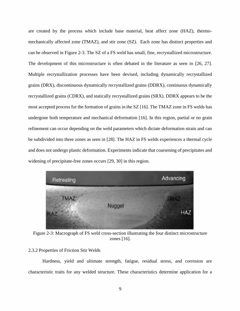
are created by the process which include base material, heat affect zone (HAZ), thermo-

mechanically affected zone (TMAZ), and stir zone (SZ). Each zone has distinct properties and

can be observed in Figure 2-3. The SZ of a FS weld has small, fine, recrystallized microstructure.

The development of this microstructure is often debated in the literature as seen in [26, 27].

Multiple recrystallization processes have been devised, including dynamically recrystallized

grains (DRX), discontinuous dynamically recrystallized grains (DDRX), continuous dynamically

recrystallized grains (CDRX), and statically recrystallized grains (SRX). DDRX appears to be the

most accepted process for the formation of grains in the SZ [16]. The TMAZ zone in FS welds has

undergone both temperature and mechanical deformation [16]. In this region, partial or no grain

refinement can occur depending on the weld parameters which dictate deformation strain and can

be subdivided into three zones as seen in [28]. The HAZ in FS welds experiences a thermal cycle

and does not undergo plastic deformation. Experiments indicate that coarsening of precipitates and

widening of precipitate-free zones occurs [29, 30] in this region.

Figure 2-3: Macrograph of FS weld cross-section illustrating the four distinct microstructure

zones [16].

2.3.2 Properties of Friction Stir Welds

Hardness, yield and ultimate strength, fatigue, residual stress, and corrosion are

characteristic traits for any welded structure. These characteristics determine application for a

10

particular material and weld configuration. All of the aforementioned properties of FS welds have

shown to be advantageous if correct operating conditions are chosen.

Hardness is a characteristic of materials which indicates its ability to resist plastic

deformation. Hardness is typically measured by employing a machine which indents the material.

Materials with high hardness values exhibit high stiffness, resistance to scratching, and ability to

resist deformation. FSW of AAs can produce hardness values higher, lower, or match that of the

base material. An important factor in determining hardness is the material’s class and condition.

For AAs, there are two distinct classes including heat-treatable and non-heat-treatable. Heat-

treatable alloys can be strengthened by precipitates, where non-heat-treatable alloys cannot. Heat-

treatable alloys include 2xxx, 6xxx, and 7xxx series alloys, and the non-heat-treatable include

1xxx, 3xxx, and 5xxx series alloys. Figure 2-4 indicates a typical hardness profile for a heat-

treatable alloy, and Figure 2-5 illustrates a typical profile for a non-heat-treatable alloy.

It is important to know the temper condition of an alloy to understand weld properties. For

alloys in the -O temper, which is the fully annealed condition, no work or grain refinement has

been applied to the material. When -O temper alloys are FS welded, work hardening and grain

refinement occurs which increases hardness. This can cause hardness and other mechanical

properties to be equal or larger than the base material, as seen in Figure 2-5. On the other hand

when non-heat-treatable work hardened alloys are FS welded, a decrease in hardness and other

mechanical properties occurs due to annealing and recovery of the microstructure. For heat-

treatable alloys that are FS welded, a decrease in hardness will occur due to the thermal cycle

which leads to precipitate coarsening and/or dissolution. In these alloys, post-weld natural aging

can occur and have been reported in [31], which showed that AA-7075 continued to harden after

11

15 years. For this reason, data for heat-treatable alloys must be critically analyzed as results may

not be indicative of the properties directly after welding.

Figure 2-4: Heat-treatable alloy FS weld hardness profile [32].

Figure 2-5: Non-heat-treatable alloy FS weld hardness profile [33].

Tensile properties are dominate traits that characterize a weld’s quality. In the literature,

reporting these traits are ubiquitous [34-40]. A compilation of multiple studies’ strength

observations with various materials can be observed in Table 2-1. In few cases, it is observed that

joint efficiency can reach 90%, and even greater than 100%; however, recalling the discussion in

12

the previous section, the material welded that reached these large joint efficiencies were alloys in

the -O temper condition.

Other key weld characteristics include fatigue, residual stress, and corrosion resistance.

These have been well documented in the literature [16, 33, 41-48] and illustrate the advantageous

qualities of FSW.

Table 2-1: Weld Strength Summary from Various FSW Studies [16].

2.4. FSW Literature Trends and Dissertation Work Significance

When FSW was initially patented, few institutions began working with the technique due

to the patent license fee. Now, many universities throughout the world have produced quality

contributions to the field. To date, according to the data base Web of Science the highest cited

articles include [16, 30, 35, 47-49] and were cited a total 4,356 times. Indeed FSW has peaked the

interests of many and will continue to flourish as a premier welding technique for industry.

However, in the literature the majority of studies are not geared toward manufacturing and how to

improve the process for production. In this doctoral work, the goal is to analyze how to improve

the manufacturing process of FSW through development of process parameter relationships to

13

defects and quality and development of a NDE system to improve efficiency that has the capability

to decrease cost for fabrication and accurately ascertain structural integrity of the welded joint.

14

CHAPTER 3 : NON-DESTRUCTIVE TESTING AND EVALUATION

The most exciting phrase to hear in science, the one that heralds the most discoveries, is not

"Eureka!" (I found it!) but "That's funny...”

-Isaac Asimov

3.1. Introduction

Welding is an essential manufacturing process performed in almost every major industry;

however, during the welding process flaws or defects can form. These defects can be found in the

form of surface or sub-surface cracks, undercut, porosity, or inclusions [50-52]; and consequently,

failure can occur from these flaws [53]. An important decision must be made regarding severity of

these weld defects and their effect on strength; therefore, weld quality and integrity are critical to

safety in an extremely wide range of products and structures. In industry, evaluation of structures

which support human life are critical to evaluate to ensure acceptable weld joints have been

fabricated.

To ensure welds have been created adequately, Non-destructive Evaluation (NDE)

techniques can be employed [54]. Different NDE methods can identify cracks, porosity,

incomplete penetration, misalignment, inclusions, and lack of fusion which all can compromise

weld strength. NDE techniques are utilized in a multitude of scenarios including: Determination

whether an object is acceptable after each fabrication step (in-process inspection), determining

whether an object is acceptable for final use (final inspection), and determining whether an existing

object already in use is acceptable for continued usage (in-service inspection). To summarize,

NDE is applied to find welding defects as well as quality assurance/quality control (QA/QC) of

welded structures [55].

The most common NDE techniques to conduct various inspections are: Ultrasonic Testing

(UT), Radiographic Testing (RT), Liquid Penetrant Testing (LPT), Magnetic Particle Testing

15

(MT), Eddy Current Testing (ECT), and Acoustic Emission (AE) testing. Each of these NDE

techniques has distinct advantages and disadvantages; consequently, depending on the application

one technique may be better suited than another. Table 3-1 briefly illustrates NDE techniques and

their principle of operation, applications, limitations, advantages, and welding defects that can be

determined. It is noted that NDE techniques rely heavily on human skills and knowledge to

correctly assess and interpret results. Proper and adequate training, developing confidence, and

appropriate certifications are required to perform non-destructive testing (NDT) [56, 57].

Therefore, flaws or defects are often dictated by a code or requirement which indicates acceptable

tolerances, i.e. The American Society of Mechanical Engineers Pressure Vessel Code [58] and

American Welding Society Structural Welding Code [59-61].

Among the number of NDE techniques, LPT, UT, and x-ray radiography are commonly

used for checking weld defects. In recent years, the conventional UT technique has been replaced

with a more reliable and technologically advanced technique of Phased Array Ultrasonic Testing

(PAUT) and Time of Flight Diffraction (TOFD). Alternatively, radiography is utilized providing

a range of techniques from traditional X-ray generators and film to newer technologies such as

Computed Radiography (CR), Direct Radiography (DR), and 3D Computed Tomography (CT).

These new technologies allow for remote visual inspection and enhancement of data visualization.

3.2. Ultrasonic Testing (UT)

Ultrasonic testing has become a widely used NDE technique with many advancements and

variations. Ultrasonic testing can be used to detect cracks, voids, and changes in geometric and

material parameters such as: thickness, stress concentration, and modulus [62]. In ultrasonic

testing, high frequency ultrasonic vibrations are generated from piezoelectric elements and thereby

transmitted into the test piece. The transmitted high frequency waves are reflected or scattered by

16

discontinuities inside the material as the waves propagate. The piezoelectric elements also act as

receivers which detect the ultrasonic reflections from the defects.

Table 3-1 : Common NDT Techniques and their applications [58].

Method Principle of

Operation Application Limitations Advantages Welding Defects

Penetrant

Testing

(PT)

Liquid dye

penetrant

application into

cracks and make

visible once

developer is applied

Surface

defects

Will not find

subsurface or

volumetric

defects

Easy and can

be used in

complex

geometry

Burn Through,

Surface Porosity,

Surface crack,

undercut

Magnetic

Particle

(MT)

Magnetic particles

are attracted to

breaks in magnetic

lines of force

Surface and

near

subsurface

defects

Not applicable

to non-magnetic

metals or alloys

Can detect

flaws up to ¼

inch below

surface

Cracks, Incomplete

penetration,

overlap

Ultrasoni

c Testing

(UT)

High frequency

ultrasound

vibrations are

introduced into

sample. Waves are

reflected or

scattered by

discontinuities

Defects

anywhere

within the

examined

volume

Sensitivity is

reduced by

rough-surface

parts; a skilled

operator is

required

Can detect

defects with

dimensions

half of the

excitation

wavelength

Cracks, Incomplete

fusion, Incomplete

penetration,

porosity, undercut

Radio-

graphic

Testing

(RT)

Penetrating rays (X-

ray or gamma rays)

cast shadows on the

other side of “solid”

objects; film

radiography records

shadow on

photographic film

Defects

anywhere

within the

examined

volume

Economic limit

to depth

penetration;

hazardous

operation;

complex shapes

are difficult to

analyze

Permits visual

analysis of

buried defects

or components

in assembly

Burn Through,

Excessive

/inadequate

reinforcement,

Incomplete

penetration,

Misalignment,

Porosity, Root

concavity, undercut

Eddy

Current

Testing

(ECT)

Constantly

measures impedance

of the probe coil;

coil impedance

changes with

material properties

and constituent

variations

Surface or

slightly

subsurface

flaws

Cannot give

absolute

measurement

only qualitative

comparison

Can be

adapted to

high-speed

production

lines

Cracks, Inclusions,

Incomplete

penetration

17

In solids, sound waves can propagate in four principle methods that are established by

particle oscillation. Sound propagates as longitudinal, shear, surface, and plate waves.

Longitudinal and shear waves are the two modes of sound propagation most commonly used in

ultrasonic testing. In longitudinal waves, the oscillations occur in the longitudinal direction or the

direction of wave propagation. In the transverse or shear wave, the particles oscillate at a right

angle or transverse to the direction of wave propagation. Three important properties of sound

waves propagating in isotropic solid materials are: wavelength (𝜆), frequency (𝑓), and

velocity (𝑉). The wavelength is directly proportional to the velocity of the wave and inversely

proportional to the frequency of the wave. This relationship is shown below in Eq. (3.1). The

wavelength is related to defect detection capabilities, which vary with ultrasonic transducer

capabilities. In general, a defect size must be larger than one-half the wavelength in order to be

detected. Therefore, if a material’s velocity remains constant, by increasing the frequency the size

of λ will decrease which results in smaller defects that can be determined.

wavelength [λ] =Velocity [V]

Frequency [f] (3.1)

The speed of sound (𝑉) within a material is a function of the properties of the material and is

independent of the amplitude of the sound wave. The general relationship between the speed of

sound in a solid and its density and elastic constants is shown in Eq. (3.2). Ultrasonic velocity is

constant for each material:

𝑉 = √𝐶𝑖𝑗

𝜌 (3.2)

where elastic constant 𝐶𝑖𝑗 is Young's modulus (𝐸), Poisson’s ratio(𝜇), or shear modulus (𝐺)

depending on the type of sound wave. When calculating the velocity of a longitudinal wave,

Young's Modulus and Poisson's Ratio are commonly used.

18

Sensitivity and resolution are two important ultrasonic properties generally used to describe

the ability to locate flaws during testing. Sensitivity is the ability to find small defects and

resolution is the ability to detect flaws that are close together within the workpiece. Generally

sensitivity and resolution of an ultrasonic probe increases with the increase of frequency. On the

other hand, as frequency increases sound tends to scatter from large or coarse grain structure and

small imperfections within a material. Before selecting an inspection frequency the material's grain

structure, thickness, discontinuity's type, size, and probable location should be considered.

During ultrasonic testing, the sound waves originate from a number of piezoelectric

elements rather than a single point. Due to multiple waves, the ultrasound intensity along the beam

is affected by constructive and destructive wave interference. The wave interference results in

variation near the source, and is known as the near-field. Because of intensity fluctuations within

this region, it is difficult to accurately estimate defect size in this region. The area beyond the near-

field where the ultrasonic beam is more uniform is called the far-field [63]. In the far-field, the

beam spreads in a pattern originating from the center of the transducer and has maximum strength.

Therefore, optimal detection results will be obtained when flaws occur in far-field area. Near-field

distance (𝑁) can be expressed as Eq. (3.3). Ultrasonic wedges helps to focus the defect in far-field

regions for thin material inspection. A schematic of near-field and far-field is shown in Figure 3-1.

𝑁 =𝐷2

4𝜆=𝐷2𝑓

4𝑉 (3.3)

𝐷 is the probe diameter, 𝑓 is the probe frequency, and 𝑉 is the material sound velocity.

The energy in the ultrasonic beam does not remain in a cylinder, but instead spreads out as

it propagates through the material. The phenomenon is usually referred to as beam-spread but is

also referred to as beam-divergence or ultrasonic diffraction. Beam spread is twice the beam

divergence, and occurs due to vibrating particles that do not transfer all energy in the direction of

19

wave propagation. Beam spread is largely determined by the frequency and diameter of the

transducer and is greater when using a low frequency transducer. As the diameter of the transducer

increases, the beam spread will be reduced. Eq. (3.4) is used to calculate beam divergence angle

(𝜃). Larger beam divergence results in over-estimation of a defect size. Figure 3-2 illustrates beam

divergence and beam spread during ultrasonic inspection.

𝑆𝑖𝑛𝜃 = 1.2𝑉

𝐷𝑓 (3.4)

Figure 3-1 : Radiated fields from an ultrasonic transducer: near-field and far-field [64].

Figure 3-2 : Beam-spread and beam-divergence during ultrasonic testing [64].

Ultrasonic technology in general can be classified into three categories: conventional

ultrasonic testing (UT), time-of-flight-diffraction (TOFD) ultrasonic testing, and phased array

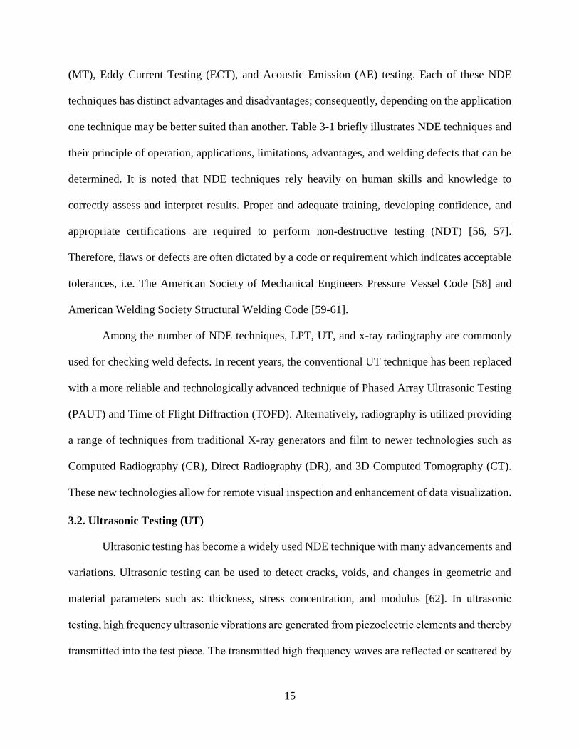
ultrasonic testing (PAUT). Figure 3-3 illustrates PAUT, TOFD, and UT configurations designed

with ESBeamTool software.

The basis of all UT inspection is A-scan data. A-scan waveforms represent the reflections

from one sound beam position in the test piece. A-scan data are used to generate other scan views

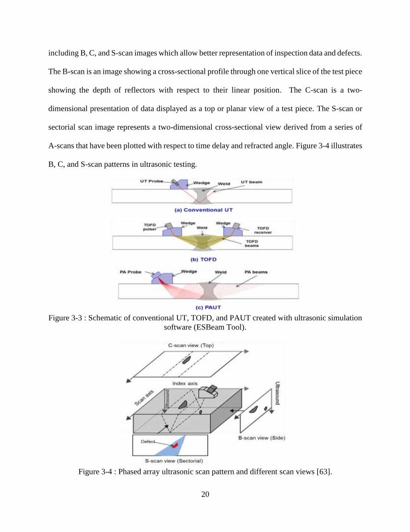
20

including B, C, and S-scan images which allow better representation of inspection data and defects.

The B-scan is an image showing a cross-sectional profile through one vertical slice of the test piece

showing the depth of reflectors with respect to their linear position. The C-scan is a two-

dimensional presentation of data displayed as a top or planar view of a test piece. The S-scan or

sectorial scan image represents a two-dimensional cross-sectional view derived from a series of

A-scans that have been plotted with respect to time delay and refracted angle. Figure 3-4 illustrates

B, C, and S-scan patterns in ultrasonic testing.

Figure 3-3 : Schematic of conventional UT, TOFD, and PAUT created with ultrasonic simulation

software (ESBeam Tool).

Figure 3-4 : Phased array ultrasonic scan pattern and different scan views [63].

21

3.3. Conventional Ultrasonic Testing

A typical ultrasonic inspection system consists of several functional units including a

transducer, wedge, and display device. The transducer is an electronic device that produces high

voltage electrical pulses. The transducer utilizing the piezoelectric elements converts the electrical

pulses into mechanical energy in the form of ultrasonic vibrations. When there is a discontinuity

in the wave path, part of the energy will be reflected back from the flaw surface. The reflected

wave signal is transformed into an electrical signal by the transducer and is displayed on a screen.

The reflected signal strength is displayed versus time. Signal travel time can be directly related to

the distance that the signal traveled. From the signal, information about the reflector location, size,

and orientation are acquired. The conventional UT method presentation of defects is obtained from

A-scan data and documentation of the defect position has to be calculated manually. Inspections

with more than one angle require sequential operations. Figure 3-5 illustrates a schematic of weld

defect detection using angle beam ultrasonic testing, and Figure 3-6 shows the corresponding A-

scan view.

Figure 3-5 : Schematic of ultrasonic method to calculate defect location [64].

For A-Scan data, an ultrasonic echo will be found between the front and back wall echoes.

For the particular material, sound velocity (𝑉) is known, and the sound path can be calculated

using Eq. (3.5).

22

𝑠𝑜𝑢𝑛𝑑 𝑝𝑎𝑡ℎ = (∆𝑡 × 𝑉)/2 (3.5)

If the reflection angle (𝜃𝑅) and material thickness (𝑇) is known, the location of the defect can be

calculated using the following equations:

𝑆𝑢𝑟𝑓𝑎𝑐𝑒 𝑑𝑖𝑠𝑡𝑎𝑛𝑐𝑒 = 𝑆𝑖𝑛𝜃𝑅 × 𝑠𝑜𝑢𝑛𝑑 𝑝𝑎𝑡ℎ (3.6)

𝐷𝑒𝑝𝑡ℎ = 𝐶𝑜𝑠𝜃𝑅 × 𝑠𝑜𝑢𝑛𝑑 𝑝𝑎𝑡ℎ (3.7)

Figure 3-6 : Typical A-scan signal indicating received signal voltage vs. time.

3.4. Time of Flight Diffraction (TOFD)

TOFD is another important variation of ultrasonic testing. In TOFD, a single element

angled beam with one pulser and receiver is used to obtain A and B scan views to represent defects.

Figure 3-7 illustrates a schematic of the TOFD process and the A and B scan views that are

acquired. TOFD images can be corrupted by incorrect setup parameters such as gain value, gate

setup, transducer separation, transducer position from weld center, and other problems such as

electrical noise [58]. At lower gain levels diffracted signals can become undetectable. At high gain

values noise increases which obscures diffracted signals leading to reduced probability of

detection. Furthermore, correct gate settings are critical because A-scan images are difficult to

interpret since there are multiple visible signals. As a minimum, the gates should cover the lateral

wave and longitudinal wave’s first back-wall signal. If the transducer separation distance is too

23

large, the back-wall and lateral wave signal weakens causing the diffracted signal amplitudes to

drop. If the transducer separation distance is too close, the lateral wave signal becomes large and

the back-wall signal becomes weak. If the transducers are not centered on the weld, the diffracted

signal amplitudes will decline to the point where flaw detection is seriously impaired. In TOFD,

the generation of noise can come from a number of sources such as electrical interference,

ultrasonic focusing depth, gain values, and coupling. Table 3-2 represents some typical welding

defects and corresponding TOFD scan views.

Figure 3-7 : Schematic of TOFD scanning process and typical TOFD A and B scan views

showing different echoes [58].

3.5. Phased Array Ultrasonic Testing (PAUT)

PAUT is relatively a new ultrasonic testing technology and decreases the level of difficulty

in determining welding defects. Ultrasonic phased arrays eventually replaced conventional

ultrasonic methods in many nondestructive evaluation applications [65-67]. Phased arrays offer

increased inspection sensitivity and coverage, as well as decreasing inspection times compared

with the conventional ultrasonic techniques using single and multi-element transducers. Another

benefit of phased array systems is the ability to produce immediate images allowing

straightforward visualization of the internal structure of a component thereby simplifying data

24

interpretation. By using PAUT technology an operator is better prepared to determine the size,

shape, and orientation of a defect versus traditional pulse echo UT techniques [68, 69].

Table 3-2 : Interpretation of Time-Of-Flight-Diffraction (TOFD) ultrasonic images [58].

Type of

Defect UT Signals Schematic and TOFD Scan view

Incomplete

root

penetration

Two signals (2, 3) from

top and bottom of the

defect

Lack of

root

penetration

More back wall signal

and inverted as

compared to lateral

wave (LW)

Side wall

lack of

fusion

Two signals from top

and bottom of the

defect

Interphases

lack of

fusion

One signals in-between

LW and back-wall

signal

Cluster

Porosity

Many small signals in-

between LW and back-

wall echoes, looks like

noise

Concave

root

Distortion of back-wall

echo

25

PAUT has three distinct components. Firstly, the probe (transducer) which functions as the

transmitter and receiver of the high frequency sound waves. Phased array ultrasonic probes utilize

an array of piezoelectric elements that in sequence generate high frequency sound waves.

Transducer frequencies are most commonly found to be in the range of 2 MHz to 10 MHz [64].

The probe is mounted on top of a wedge component which couples the sound waves generated by

the probe to the work piece. Wedges are used to steer the sound waves at a certain angle as they

enter the work-piece according to Snell’s Law. The couplant, typically a moderately viscous,

nontoxic liquid or gel, is used between the wedge and the work-piece to facilitate the transmission

of sound energy between the wedge and the test piece. Lastly, a data acquisition unit is used to

generate images that can utilize the sound waves to determine defects of a material. These data

acquisition units are very sophisticated and have many input variables that will affect the images

produced. In Figure 3-8 , an illustration is given of a probe/wedge unit that is situated on top of

a FS weld with a defect located on the upper AS. During one firing sequence, each element is

engaged beginning in the direction of the arrow starting from A and ending at B (shown on the

probe). With the associated wedge angle and firing sequence a wave front is created following

Huygen’s interference patterns [70] allowing defects to be found in a large area. For simplicity

only the “first leg” of the wave front is illustrated. In practical applications, one can use multiple

legs and can view larger swept areas.

For PAUT inspection, multiple input parameters must be entered into the data acquisition

unit to accurately determine defect sizes and locations. These variables include the characteristics

of the transducer, wedge, and welded area. Setup variables also include parameters that assist in

generating an accurate focal law for the high frequency sound waves. These parameters include

scan type, wave type, number of elements to be viewed, beam angle, and gate settings. Lastly, one

26

of the most important procedures that need to be conducted is calibration. Different types of

calibration blocks (ASTM, PACS, IIW, NAVSHIP, etc.) are utilized depending on the application

and defect code. Calibration blocks should be made of the same material that is to be inspected

[71]. In the calibration procedure, many steps are required that have to be followed in a particular

order to allow for the system to calculate correct wave characteristics. In general, three procedures

have to be conducted. These include the material velocity, wedge delay, and sensitivity

calibrations. In the calibration three different types of reflectors can be used to verify velocity and

wedge delay variables which include radius, depth, and thickness. If one is using an angle-beam

wedge, the radius and depth reflectors must be utilized; however, if a 0 degree wedge is employed

then the thickness reflector (back-wall reflection) can be used.

Figure 3-8 : A typical probe and wedge configuration with illustration of wave propagation

inside a FS welded specimen.

The sound waves are predictable due to wave physics principles. These wave principles

are classical physics phenomena and have been well documented as they pertain to ultrasonics, as

seen in [72-79]. Work has also been conducted to determine the effect of element size in linear

phased arrays [80]. Optimization of PAUT probe design has likewise been discussed in [81, 82].

Simulations of PAUT systems have been conducted to predict phased array ultrasonic wave

interactions and behavior inside materials in [83, 84]. With this new technology, simulation

27

software has been developed to aid in the scanning process to create the required PAUT software

to accurately detect defects. A requirement is to describe the inspection task and enter fundamental

information such as site location, number of welds, pipe diameter, thickness, material properties,

weld preparation, procedure, and ultrasonic method to be used. The software will then calculate

and generate all the UT set-up parameters required to perform phased array inspection of the weld.

As mentioned earlier the most common scan views (images) that a PAUT system utilizes

are A, B, C, and S scans. If there is a defect present in the scanned samples, it can be visualized

with 6-dB color change [70, 71, 85]. Figure 3-9 shows typical A, S, and C-scan views obtained

from phased array ultrasonic testing. The S-scan is perhaps the most useful asset to current PAUT

post-weld evaluation due to the ability to steer the sound waves in a range of angles which allows

for easy visualization of a specimen [66]. The horizontal axis corresponds to location of the defect

from probe position, and the vertical axis to depth of the test piece. During inspection, the

inspection data for each weld is stored into the memory. The location can be identified by

incorporating an encoder or scanner. After inspection, a sophisticated software package is

employed allowing a qualified ultrasonic inspector to review and analyze the inspection data

utilizing advanced analysis tools such as: real time volume corrected imaging, as well as,

conventional image analysis, image enhancement, and measurement determination.

Figure 3-9 : PAUT A, S, and C-scan view acquired using Olympus Omniscan MX2.0 data

acquisition unit [63].

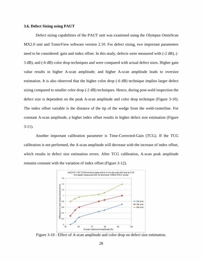
28

3.6. Defect Sizing using PAUT

Defect sizing capabilities of the PAUT unit was examined using the Olympus OmniScan

MX2.0 unit and TomoView software version 2.10. For defect sizing, two important parameters

need to be considered: gain and index offset. In this study, defects were measured with (-2 dB), (-

3 dB), and (-6 dB) color drop techniques and were compared with actual defect sizes. Higher gain

value results in higher A-scan amplitude; and higher A-scan amplitude leads to oversize

estimation. It is also observed that the higher color drop (-6 dB) technique implies larger defect

sizing compared to smaller color drop (-2 dB) techniques. Hence, during post-weld inspection the

defect size is dependent on the peak A-scan amplitude and color drop technique (Figure 3-10).

The index offset variable is the distance of the tip of the wedge from the weld-centerline. For

constant A-scan amplitude, a higher index offset results in higher defect size estimation (Figure

3-11).

Another important calibration parameter is Time-Corrected-Gain (TCG). If the TCG

calibration is not performed, the A-scan amplitude will decrease with the increase of index offset,

which results in defect size estimation errors. After TCG calibration, A-scan peak amplitude

remains constant with the variation of index offset (Figure 3-12).

Figure 3-10 : Effect of A-scan amplitude and color drop on defect size estimation.

29

Figure 3-11 : Effect of index offset and color drop on defect size estimation (fixed gain value).

Figure 3-12 : Variations of A-scan amplitude with index offset to illustrate the effect of TCG

calibration.

To find the detectability and defect sizing capability of PAUT, varying sizes (0.79 mm,

1.58 mm, 1.98 mm, 2.38 mm, 2.78 mm, 4.76 mm, and 6.35 mm diameters) of seven holes were

prepared on an AA6061-T651 plate and scanned with a calibrated PAUT unit. Figure 3-13 shows

the C-scan view of the plate with varying-hole sizes. The PAUT unit can precisely detect the sizes

and locations of the holes. To identify the defect sizing precision and accuracy of PAUT, different

size side-drilled-holes (SDH) were bored into an AA-2219 block at varying depths and were

measured. The variation in measurement is shown in Table 3-3. Absolute error in height, depth,

30

and location sizing was 0.24±0.20, 0.28±0.18, and 0.46±0.17 respectively. It is generally accepted

that the tolerance for PAUT is 0.5-1.0 mm depending on how stringent the application requirement

[62]. It is observed that there is overestimation for thicker plates and underestimation for thinner

plates. This exemplifies one of the characteristics of waves propagating through a material. For a

defect at larger thicknesses, the sound waves travel a larger distance which causes the wave to

expand. This results in the elongation of the defect image; alternatively, for defects at smaller

depths, the wave does not reach its focal length and thereby underestimates the defect. In other

words the defect image depends on the near and far fields focusing distances of the wave.

Figure 3-13 : Aluminum alloy plate with seven varying hole sizes with associated C-scan and

eco-dynamic A-Scan images.

Table 3-3 : Comparison of Defect Sizing of PAUT.

Thickness

(mm)

Actual

Dia.

(mm)

Meas.

Dia.

(mm)

Δ

Dia.

(mm)

Actual

Depth

(mm)

Meas.

Depth

(mm)

Δ

Depth

(mm)

Actual

Dist.

(mm)

Meas.

Dist.

(mm)

Δ

Dist.

(mm)

25.5 2.8 3.1 0.3 8.1 8.25 0.15 16.1 16.6 0.5

25.5 2.8 3 0.2 14.1 14.2 0.1 10.8 11.4 0.6

25.5 1.6 2.2 0.6 11.8 11.9 0.1 17.9 18.3 0.4

25.5 3.5 3.6 0.1 12.5 11.9 -0.6 18.5 19.0 0.5

8.35 1.6 1.5 0.1 4.2 3.9 -0.3 4.1 3.6 -0.5

8.35 2.4 2.0 -0.4 4.2 3.8 -0.4 3.6 3.0 -0.6

8.35 2.8 2.8 0 4.5 4.2 -0.3 12.5 12.4 -0.1

31

3.7. Radiographic Testing (RT)

One of the widely used NDT methods for volumetric examination is radiography. In

radiography, X-rays or gamma-rays are used to produce a radiographic image obtaining

differences in thickness, defects (internal and surface), and changes in structure. The procedure for

producing a radiograph is to have a source of penetrating radiation (X-rays or gamma-rays) on one

side of a specimen to be examined and a detector of the radiation (radiographic film) on the other

side, see Figure 3-14.

Figure 3-14 : Schematic of Basic Set-up for film radiography [86].

Different radioactive materials and X-ray generators produce radiation at different energy

levels and at different rates. It is important to understand the terms used to describe the energy and

intensity of the radiation. The energy of a single wavelength X-ray can be calculated by the Eq.

(3.8).

𝐸 = ℎ. 𝜗 =

ℎ𝑐

𝜆

(3.8)

Where 𝐸 is the energy, ℎ is Planck’s constant, 𝜗 is frequency, c is velocity of electromagnetic

radiation, and 𝜆 is the wavelength. The energy of the radiation is responsible for its ability to

penetrate matter. Higher energy radiation can penetrate more and higher density matter than low

32

energy radiation. Radiation intensity is the amount of energy passing through a given area that is

perpendicular to the direction of radiation travel in a given unit of time. Presently, a wide range of

industrial radiographic equipment, image forming techniques, and examination methods are

available. Similar to ultrasonic NDE methods, knowledge and experience are needed to select the

appropriate method for a particular application. Generally for weld inspection, the methodology

will follow ASTM-E1032 standards [87] with associated safety requirements [59]. The

radiographic sensitivity shall be judged based on a penetrometer or wire image quality indicator

(IQI). The results of the X-ray image produce a two dimensional representation of the specimen.

In a radiographic film, darkness of the film vary according to the amount of radiation that has

reached the film through the test object. In radiographic film, darker areas indicate more exposure

and lighter areas indicate less exposure. The processed film is usually viewed by placing in front

of a screen providing white light illumination of uniform intensity. The light is transmitted through

the film and the image can be observed. The term “radiographic density” is a measure of the degree

of film darkening. Radiographic density is the logarithm of two measurements: the intensity of

light incident on the film (𝐼0) and the intensity of light transmitted through the film (𝐼𝑡 ).

𝑅𝑎𝑑𝑖𝑜𝑔𝑟𝑎𝑝ℎ𝑖𝑐 𝑑𝑒𝑛𝑠𝑖𝑡𝑦 = log(

𝐼0𝐼𝑡)

(3.9)

One important challenge of radiographic analysis is the data interpretation and defect

classification. For this reason, X-ray images that are acquired are compared with standard

radiographic images [86].

33

CHAPTER 4 : EXPERIMENTAL FACILITIES, TOOLING, AND

WELDING METHODOLOGY

We are what we repeatedly do... excellence, therefore, isn't just an act, but a habit and life isn't

just a series of events, but an ongoing process of self-definition.

-Adapted from Aristotle

4.1. Facilities

The facilities and welding methodology utilized in this doctoral research are presented in

this chapter. Additionally, a description of the control settings utilized during welding is discussed

and the methodology for determining the classification of the welded joint is provided.

4.1.1 Michoud Assembly Facility

The NASA Michoud Assembly Facility (MAF) is a national asset worth over 3 billion

dollars on 832 acres located on an intercostal waterway. The main plant floor at MAF has 1.3

million square feet of manufacturing space. MAF has a rich history, starting out as a French royal

land grant which became a sugar cane plantation operated by Antoine Michoud [88]. In 1940, the

U.S. government acquired the land and built a production facility for cargo aircraft, tank engines,

and other structures. Then, in 1961, NASA acquired the property to build the core stages for Saturn

V rockets [88]. From 1981-2011, MAF was employed for constructing the external tanks ETs for

NASA’s Space Shuttle. Through Shuttle’s history, three ET variants were built including ET,

lightweight ET, and super lightweight ET. The original ET weighed approximately 76,000 lbs.

dry. The lightweight ET weighed 66,000 lbs., and the last variation reduced the weight by roughly

7,000 lbs. [89].

MAF houses the National Center for Advanced Manufacturing (NCAM). NCAM, founded

in 1999, is a partnership between NASA, the state of Louisiana, Louisiana State University (LSU),

the University of New Orleans (UNO), and the UNO Research and Technology Foundation. The

purpose of NCAM is to develop advance manufacturing technologies to support NASA space

34

programs and adjacent industries and provide a link between academic research. NCAM houses a

state-of-the-art FSW facility with the world’s most robust FSW platforms. These platforms include

Process Development System (PDS), Universal Weld System (UWS), and Robotic Weld Tool

(RWT).

Through the entirety of this doctoral work MAF facilities were employed, specifically

employing I-STIR PDS and UWS FSW machines as seen in Figure 4-1. The PDS system is mainly

employed for weld development. On the other hand the UWS, currently utilized for manufacturing

the Orion Capsule, is a production system.

Figure 4-1 : Weld platforms employed throughout the experimental program (Courtesy NCAM).

4.1.2. Louisiana State University

LSU, founded in 1876, was Louisiana’s first land-grant institution committed to teach

military tactics, engineering and agriculture. In 1902, LSU expanded its engineering program to

include mechanical engineering [90]. LSU’s mechanical engineering department currently houses

a materials testing lab which contains multiple systems to characterize materials. These facilities

were employed for mechanical testing, material preparation and characterization.

35

In this study, for tensile mechanical property testing an 810 Material Test System was

employed. The test coupons were prepared according to AWS specification for FSW of AAs and

tested at room temperature using a displacement rate of 1.0 mm/min according to ASTM E8/8M-

11. The tensile strain was measured using a 25.4 mm (1″) gauge length extensometer which was

attached to the middle of the specimen near the weld zone. Tensile toughness values were

calculated from the area under the tensile stress-strain curve. The yield strength obtained employed

the 0.2% offset yield strength method.

For hardness testing, a FUTURE-TECH Rockwell system, Model Digital FR-3e was

employed (Figure 4-3). To better understand the welding effects on metallurgical and

microstructural changes, the hardness values across the weld surface were measured. For a weld

joint, hardness values are usually sensitive to welding condition, welding process, heat input,

preheat or inter-pass temperature, and plate thickness. Before hardness testing, the welded

specimens were grounded and polished. For aluminum alloys, 1.58 mm (1/16 inch) diameter steel

ball indenter was utilized. Before using the micro-hardness tester, it was calibrated utilizing an

appropriate calibration block. Hardness values were taken to correlate with tensile and fatigue

strength of the welded specimens.

Polishing and grinding tasks utilized a Buehler 250 MetaServe with magnetic platen bases

as seen in Figure 4-4. Polishing pads that were utilized had magnetic bases, and entailed the diamat

and white polishing pad series from AlliedTech. Welded specimens were ground with diamond

suspensions (9µm to 0.25µm) following ASTM E3-11 standard [91] and then mirror polished. The

coupons were then chemically etched according to ASTM E407-07 standard [92] to reveal the

microstructure. The etchant employed was Keller reagent (1 mL HF, 1.5 mL HCL, 2.5 mL HNO3,

95 mL H2O). For micro and macro inspection of welds, a metallographic digital light optical

36

microscope (OM) was employed (Figure 4-5). In order to cut the tensile and microstructure

coupons a band saw was utilized as seen in Figure 4-6.

Figure 4-2: MTS-810 uniaxial tensile test set-up including hydraulic unit wedge grips, a FSW

tensile specimen, and an MTS extensometer.

Figure 4-3 : FUTURE-TECH Rockwell Hardness Tester.

Figure 4-4: MetaServe 250 Polisher/Grinder employed through the doctoral work.

37

Figure 4-5 : Metallurgical microscope utilized for microstructural analysis.

Figure 4-6 : Band Saw utilized for cutting FS welded tensile and macro coupons.

After welding, panels were tested with non-destructive evaluation (NDE) techniques

including PAUT, X-ray radiography, and liquid dye penetration tests. For PAUT inspection, an

OMNIScan MX2 data acquisition unit was employed as seen in Figure 4-7. Throughout the work

a variety of transducers and wedges were employed for weld quality inspection. A sample of the

typical devices utilized can be observed below in Figure 4-8. For specimens that were tested with

X-ray radiography, a local company was contracted to complete the work. For liquid dye penetrant

testing, MAGNAFLUX products were employed as seen in Figure 4-9.

38

Figure 4-7: OMNIScan MX2 Data acquisition system employed for PAUT inspection through

the entirety of this work.

Figure 4-8: Select PAUT transducers and wedges employed through the work. Going from left to

right: Olympus Weld Series 5L32-A31 transducer with SA31-55S wedge, Olympus 10L32-A10

transducer with SA10-N55S wedges, Olympus 10L32-A10 with custom casing and two in-house

high-temperature wedges.

Figure 4-9: Liquid dye penetrant testing equipment employed for weld surface defect

examination.

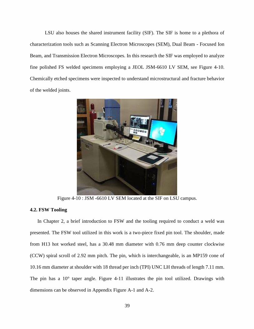
39

LSU also houses the shared instrument facility (SIF). The SIF is home to a plethora of

characterization tools such as Scanning Electron Microscopes (SEM), Dual Beam - Focused Ion

Beam, and Transmission Electron Microscopes. In this research the SIF was employed to analyze

fine polished FS welded specimens employing a JEOL JSM-6610 LV SEM, see Figure 4-10.

Chemically etched specimens were inspected to understand microstructural and fracture behavior

of the welded joints.

Figure 4-10 : JSM -6610 LV SEM located at the SIF on LSU campus.

4.2. FSW Tooling

In Chapter 2, a brief introduction to FSW and the tooling required to conduct a weld was

presented. The FSW tool utilized in this work is a two-piece fixed pin tool. The shoulder, made

from H13 hot worked steel, has a 30.48 mm diameter with 0.76 mm deep counter clockwise

(CCW) spiral scroll of 2.92 mm pitch. The pin, which is interchangeable, is an MP159 cone of

10.16 mm diameter at shoulder with 18 thread per inch (TPI) UNC LH threads of length 7.11 mm.

The pin has a 10° taper angle. Figure 4-11 illustrates the pin tool utilized. Drawings with

dimensions can be observed in Appendix Figure A-1 and A-2.

40

Figure 4-11: Pin Tool employed during FSW experiments (top) and interchangeable threaded pin

(bottom).

In order to conduct a FS weld a rigid fixture is required to hold the material to be welded. The

fixture utilized for welding in this work employed a steel anvil. The anvil is the structure that reacts

the load applied by the tool in the downward direction. Steel bars (often considered chill bars)

were placed on the AS and RS panels 38.1 mm away from weld centerline and rigidly held in place

with four clamps. Side compression screws were used on the RS to ensure the panels would not

slide and ensure the faying surfaces of the workpieces were in intimate contact. The fixture utilized

can be observed in Figure 4-12.

Figure 4-12: FSW fixture employed during weld operations.

AA Panel

Clamp

Anvil

Chill Bar

41

4.3. FS Weld Experimental Methodology

Two AA-2219-T87 panels with dimensions 609.6 mm long, 152.4 mm wide, and 8.13 mm

thick were welded in a typical butt-joint configuration through the entire study. The material was

chosen based upon direction provided by NASA, as this material is often used in production of

their flight hardware. Before welding the panels were lightly ground to remove oxide particles.

This process is conducted to mitigate entrapment of said particles which can lead to weld defects.

The panels were then wiped with an alcohol solution and inserted into the fixture. The welds

employed a 0° lead angle with zero index-offset from the centerline, with no mismatch, peaking

or gap. At the onset of the study, NCAM and MAF employees aided in conducting the FS weld

experiments. During these welds the author was trained in operation of the FSW machines. After

completing operation training, the author conducted the remaining welds in the study.

With any welding process, determination of acceptable ranges of process parameters that

can be used for a pin tool, fixture, and material must be determined. FSW conditions can greatly

change when any of these variables are altered. For this reason, at the onset of the research, two

welds were conducted with the FSW fixture (provided by NCAM), material, and pin tool type to

illuminate appropriate process parameter ranges by utilizing the position-control setting on the FS

welding machine. Based on prior experience, spindle rotational speeds and feedrates were

estimated and employed. Consequently, a range of appropriate plunge force values were

determined by comparing pin penetration depth. FSW experiments were thereby conducted in the

rest of the work with the load-control setting allowing the three process parameters to be varied

individually. Typically in manufacturing environments, weld schedules for a particular welding

configuration have been optimized and deemed acceptable based upon numerous trials. In this type

of environment, the outcome of a weld is well known and load-control is utilized which provides

42

precise control of welding parameters and achieves steady-state welding conditions throughout the

weld. This practice minimizes weld force and process parameter signal variation. As the current

study is employing logic of eventually controlling all three parameters and their effects on weld

result, load-control was utilized.

43

CHAPTER 5 : FSW AA-2219 LITERATURE REVIEW

Success consists of going from failure to failure without loss of enthusiasm.

-Winston Churchill

5.1. Introduction

Aluminum Alloys (AAs) are widely employed in aerospace applications due to their

notable strength and ductility. The extension of good strength and ductility to cryogenic

temperatures make AAs suitable for liquid oxygen and hydrogen oxidizer rocket fuel tankage. AA-

2219, a descendent of the original duralumin used to make Zeppelin frames, is currently in wide

use in the aerospace industry. It is an aluminum-copper alloy. Copper hardens the alloy by

precipitation of Al2Cu. The Space Shuttle ET was fabricated from AA-2219 until the still stronger

aluminum-lithium alloy AA-2195 replaced it, but the more economical AA-2219 alloy remains in

use.

The FSW process, a solid-state process, was implemented by NASA as a response to fusion

welding problems introduced by AA-2195. The FSW process joins the surfaces of a butt-weld

seam by stirring the surfaces together with a pin while the metal is held in place by a shoulder. The

FSW process consistently produced stronger, more robust welds, supplanted the Variable Polarity

Plasma Arc Welding (VPPAW) process for the Space Shuttle ET, and has been widely adopted in

the aerospace industry.

At the onset of this work, a literature review was conducted to ascertain pertinent FSW

works that employ AA-2219. AA-2219 is often used in manufacturing, especially for aerospace

applications in various thicknesses, temper conditions, and tool configurations. It is advantageous

for the researcher to understand the works that have been conducted in their field, not only to gain

knowledge and understand intricacies of the application, but also ensure those works are not

44

repeated. For this reason, the review is followed by observed trends that were found in the

literature.

5.2. Literature Review on FSW of AA-2219

A review of literature available in public domain is presented in this section. The review

analyzes material condition and thickness, FSW tool and machine type, process parameter ranges,

number of weld schedules, and key conclusions. These properties have been deemed important to

understand the extent of a FSW study and are thereby listed. The review is divided into multiple

sections in order to group similar topics as seen in Tables 5-1 – 5-6. Firstly, works conducted

analyzing effects of varying process parameters, weld defects, and mechanical properties are

reported. Secondly, studies including residual stress, fatigue, and post-weld heat treatment

(PWHT) are presented. Corrosion works are provided after. Fourthly, experiments of dissimilar

materials including AA-2219 are reviewed. Thereafter, works comparing FSW of AA-2219 with

fusion techniques are described, followed by research into non-conventional FSW processes and

special studies. Finally, research trends in the subject area are discussed in the following section.

5.2.1 Evaluation of Literature Trends in FSW of AA-2219

Trends in FSW literature have appeared and are discussed herein. One trend observed is

lack of identification of material condition. The temper designation is important for researchers to

compare work conducted with other studies. For instance, a material’s strength after welding will

decrease due to microstructural degradation in heat treatable alloys. For non-heat treatable alloys,

especially in the -O condition, higher strengths than the parent material can be attained due to

microstructural refinement and work caused by the welding process. A material’s temper

designates its initial strength and is the basis for measuring strength reduction/addition which is

essential for weld characterization. Furthermore, the reasoning a certain temper employed is

45

seldom discussed. The cause may stem from limitations on material availability; however,

employing a certain temper condition will affect properties of a weld, such as process parameter

operating window, and is key to the application it will be employed. As an example, AA-2219 in

the T87 condition provides better ultimate tensile and yield strength compared to other heat

treatments [93].

Secondly, description of procedures and conditions involved during welding are often

briefly discussed. In FSW, numerous variables affect the outcome of a weld. For example, detailed

descriptions of the pin tool, process parameters, and control settings are often overlooked when a

study is presented. Studies seldom show descriptions of machine or fixture utilized for welding.

The welding machine is important as FSW requires large forces which need to be properly

controlled. FSW is a costly endeavor, and for this reason university studies are quite limited due

to these constraints. Therefore, innovative approaches have been taken to circumvent this issue.

One such method is to utilize milling machines that have been converted into FSW machines. This

practice however, has never been evaluated in the literature as to whether it affects FSW results.

For instance, control settings of the machine are critical to monitor FSW plunge force, spindle

rotational speed, and feedrate during welding. With non-conventional or converted welding

machines, process parameters may be inaccurate or have large deviations that could produce

inconsistent data. Flight hardware would never be welded with a converted milling machine.

Additionally, the fixture utilized for FSW is typically never discussed. A fixture holds down the

workpiece to be welded and consequently acts as a heat sink. Typically steel anvils are employed

in tandem with rigid steel bars to hold down the workpiece. As heat transfer is very important in

FSW, these key parameters should as well be documented so that comparisons can be made.

46

Another tendency that can be questioned in FSW literature is process parameter and

operating window selection. These features are seldom discussed for a particular pin tool and

welding condition. Any given pin tool has an operating window, and commonly in research these

boundaries look to be exceeded.

According to the Web of Science data base (9-18-2017), using key words friction stir

welding and AA-2219, only 1.9% of the FSW literature employed AA-2219. As this alloy is

generally employed in industry, such as for Orion Crew Module and SLS propellant tankage, the

works to date have been compiled. Among the existing literature none showed extensive

investigations to provide a complete scenario of welding conditions and process parameters.

47

Table 5-1 : Process Development and Mechanical Properties.

(FSW – friction stir welding, FFSW - filling friction stir weld, SR-FSW – self-reacting friction stir weld, FSSW – friction stir spot

weld, FSP – friction stir processing, PWHT - post weld heat treatment, RS – retreating side, AS – advancing side, WZ – weld zone,

TMAZ – thermo-mechanical affected Zone, HAZ – heat affected zone, BM - base metal, NRS – non-rotational shoulder, GTAW – gas

tungsten arc weld, EBW – electron beam weld, RDR – reverse double rotation, PAUT – phased array ultrasonic testing)

Ref Condition Thickness Tool - Machine Parameter

Range

Weld

Schedules Key Points

[94] T87 8 mm

Conventional -

Indigenous

designed

machine

500-1500

RPM

30 – 150

mm/min

12 kN

22 Development of operating window

for defect free welds

[95] T87 7 mm

Conventional -

ESAB FSW

Machine

200 -300

RPM

300 – 500

mm/min

24.5 – 34.3

kN

27 UTS and percentage elongation

increases with increase in plunge

force

[96] T87 5 mm

Conventional -

Adapted

Milling

Machine

250 – 400

RPM

60 – 180

mm/min

NA

27

Plunge force readings are greatly

affected by shoulder diameter and

slightly affected by rotational and

welding speeds

[97] NA 10.16 mm

Conventional -

Horizontal

Weld Tool at

MSFC

200 – 400

RPM

NA

NA

4

Plunge phase investigation

Experimental plunge force

and torque readings agree

well with developed model

(table cont’d)

48


Range

Weld


[98] O 14 mm Conventional -

NA

300 – 600

RPM

60 -100

mm/min

NA

NA

An increase in rotational and

decrease in feedrate causes larger

heat input into system

Grain size at top of weld is coarser

than at bottom

[99] T6 17 – 19

mm

Conventional -

NA

210 – 300

RPM

80 – 150

mm/min

NA

14

Evaluation of FSW defects with

NDE techniques: x-ray, PAUT, and

fluorescent penetrating fluid by

varying rotational and feedrate

[100] O 5 mm Conventional -

NA

800 RPM

200 mm/min

NA

1

Comparison of oxide defect on as-

welded and PWHT specimens

PWHT joints with oxide defect

degrades mechanical properties

[101] T87 6.35 mm Conventional -

NA

150 – 300

RPM

76 – 152

mm/min

29 – 36 kN

9

Tungsten wire tracer study

Material entrained in rotating plug is

subjected to large thermo-

mechanical effects

[102] T6 7.5

Conventional -

FSW machine

(FSW-3LM-

003)

300 – 1000

RPM

50 – 400

mm/min

NA

10

Increase in rotational or increase in

feedrate produces larger tensile

properties until a plateau, which then

after sharply decrease

(table cont’d)

49


Range

Weld


[103]

T6 6 mm

Conventional -

NA

800 – 1300

RPM

100 – 140

mm/min

NA

6 Second-phase particle size decreases

and grain size increases as rotational

speed increases

[104] T62 12 mm Conventional -

NA

300 – 500

RPM

60 – 100

mm/min

NA

4

Close to the shoulder larger grains

are found compared to grains at the

root of the weld

Pin profile has little effect on tensile

properties, but feedrate and

rotational speed have greater effects

[105] O and T6 NA Conventional -

NA

800 RPM

60 – 500

mm/min

NA

NA Base material conditions greatly

affect the welding morphology and

tensile properties

[106] T87 6 mm

Conventional -

Indigenous

designed

machine

1400 – 1800

RPM

15 – 75

mm/min

8 – 16 kN

31

A square pin profile produced

superior tensile properties

Response Surface Method and

Hooke and Jeeves algorithm

employed to predict tensile strength

with a 95% confidence level

(table cont’d)

50


Range

Weld


[107] T87 6 mm

Conventional -

Indigenous

designed

machine

1400 – 1800

RPM

15 – 75

mm/min

8 – 16 kN

31

A square pin profile produced

superior tensile properties

A mathematical relationship was

developed using ANOVA and

regression analysis

[108] T87 6 mm

Conventional -

Indigenous

designed

machine

1600 RPM

22.2 – 75

mm/min

12 kN

4

Comparing five pin profiles, the

square profiled pin produced defect

free regions at all welding speeds

Comparing three welding speeds,

45.6 mm/min produced superior

tensile results

[109] T87 6 mm

Conventional -

Indigenous

designed

machine

1500 – 1700

RPM

45.6 mm/min

12 kN

3 1600 RPM produced superior tensile

properties regardless of pin profile

[110] T87 5 mm

Conventional -

Adapted CNC

milling

machine

NA NA Roughly 40% of Al2Cu precipitates

in WZ dissolved compared to base

material


NA

800 RPM

200 mm/min

NA

1

The level of dissolution of dissolved

precipitates in WZ is higher than

TMAZ

In HAZ there is only coarsening of

metastable precipitates

(table cont’d)

51


Range

Weld


[112] T87 6 mm

Conventional -

Indigenous

designed

machine

1400 - 1700

RPM

50 – 100

mm/min

8 – 12 kN

5

Experimental correlations was

established to predict tensile

strengths of welded specimens with

95% confidence levels


NA

300 RPM

80 mm/min

NA

1

Water cooled FSW resulted in

greater refinement of grain sizes in

WZ

Water cooling found to have higher

tensile properties than air-cooled

welding

[114] T87 10 mm

Conventional -

NA

NA NA

Environmental Crack Susceptibility

is similar for all weld microzones

and unaffected by parent material

FS welds are more corrosion

resistant than parent material

[115] T87 8.3 mm

Conventional -

MTS FSW

process

development

system

NA

76.2 mm/min

NA

NA

Torque and rotational speed used to

develop optimum process parameters

for a given alloy

Estimation of magnitude of strain

rate found to be > 20 s-1


NA

800 RPM

180 mm/min

NA

NA

Fatigue properties examined by

experimental and numerical analysis

Maximum equivalent plastic strain

location identified during stress-

controlled loading

(table cont’d)

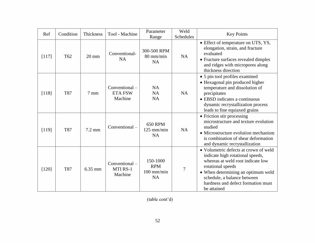
52


Range

Weld


[117] T62 20 mm Conventional-

NA

300-500 RPM

80 mm/min

NA

NA

Effect of temperature on UTS, YS,

elongation, strain, and fracture

evaluated

Fracture surfaces revealed dimples

and ridges with micropores along

thickness direction

[118] T87 7 mm

Conventional –

ETA FSW

Machine

NA

NA

NA

NA

5 pin tool profiles examined

Hexagonal pin produced higher

temperature and dissolution of

precipitates

EBSD indicates a continuous

dynamic recrystallization process

leads to fine equiaxed grains

[119] T87 7.2 mm Conventional –

650 RPM

125 mm/min

NA

NA

Friction stir processing

microstructure and texture evolution

studied

Microstructure evolution mechanism

is combination of shear deformation

and dynamic recrystallization

[120] T87 6.35 mm

Conventional –

MTI RS-1

Machine

150-1000

RPM

100 mm/min

NA

7

Volumetric defects at crown of weld

indicate high rotational speeds,

whereas at weld root indicate low

rotational speeds

When determining an optimum weld

schedule, a balance between

hardness and defect formation must

be attained

(table cont’d)

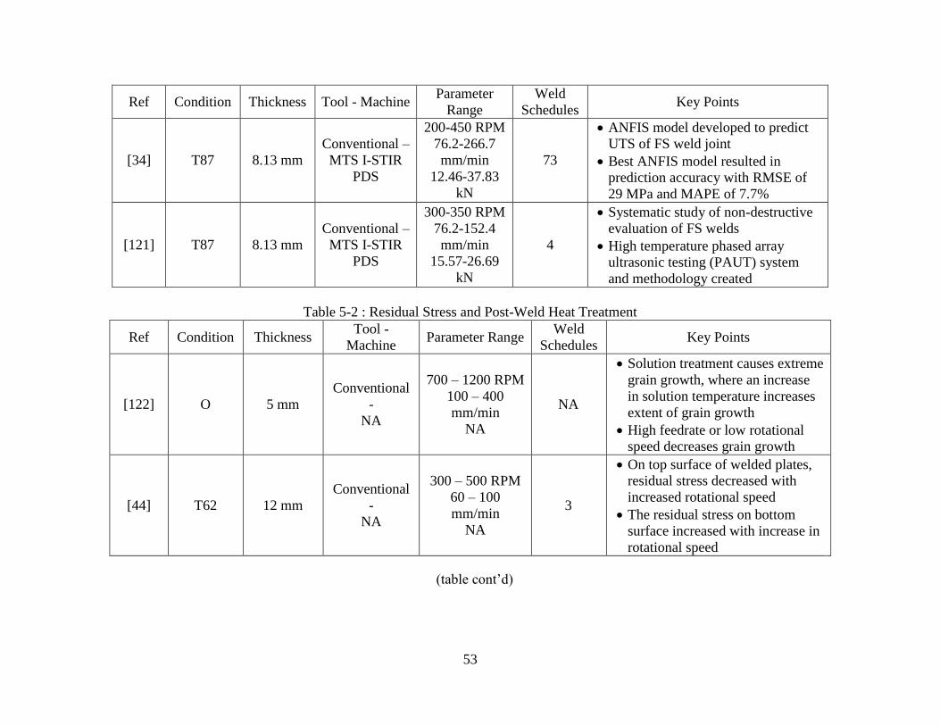
53


Range

Weld


[34] T87 8.13 mm

Conventional –

MTS I-STIR

PDS

200-450 RPM

76.2-266.7

mm/min

12.46-37.83

kN

73

ANFIS model developed to predict

UTS of FS weld joint

Best ANFIS model resulted in

prediction accuracy with RMSE of

29 MPa and MAPE of 7.7%

[121] T87 8.13 mm

Conventional –

MTS I-STIR

PDS

300-350 RPM

76.2-152.4

mm/min

15.57-26.69

kN

4

Systematic study of non-destructive

evaluation of FS welds

High temperature phased array

ultrasonic testing (PAUT) system

and methodology created

Table 5-2 : Residual Stress and Post-Weld Heat Treatment

Ref Condition Thickness Tool -

Machine Parameter Range

Weld


[122] O 5 mm

Conventional

-

NA

700 – 1200 RPM

100 – 400

mm/min

NA

NA

Solution treatment causes extreme

grain growth, where an increase

in solution temperature increases

extent of grain growth

High feedrate or low rotational

speed decreases grain growth

[44] T62 12 mm

Conventional

-

NA

300 – 500 RPM

60 – 100

mm/min

NA

3

On top surface of welded plates,

residual stress decreased with

increased rotational speed

The residual stress on bottom

surface increased with increase in

rotational speed

(table cont’d)

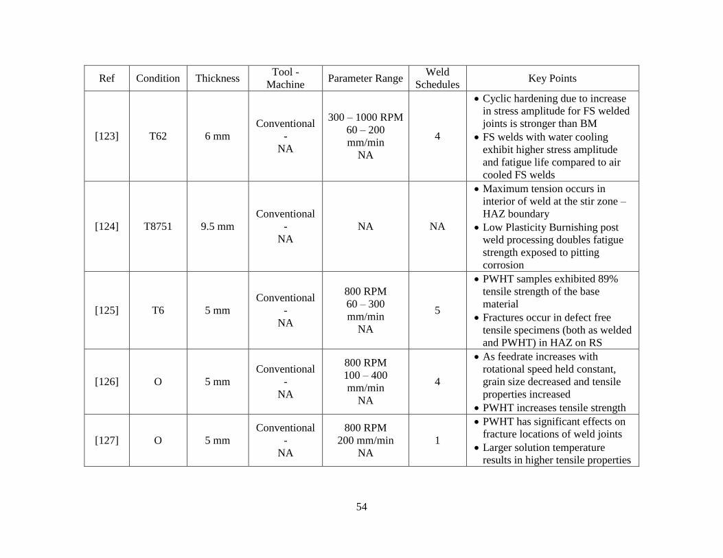
54



Weld


[123] T62 6 mm

Conventional

-

NA

300 – 1000 RPM

60 – 200

mm/min

NA

4

Cyclic hardening due to increase

in stress amplitude for FS welded

joints is stronger than BM

FS welds with water cooling

exhibit higher stress amplitude

and fatigue life compared to air

cooled FS welds

[124] T8751 9.5 mm

Conventional

-

NA

NA NA

Maximum tension occurs in

interior of weld at the stir zone –

HAZ boundary

Low Plasticity Burnishing post

weld processing doubles fatigue

strength exposed to pitting

corrosion

[125] T6 5 mm

Conventional

-

NA

800 RPM

60 – 300

mm/min

NA

5

PWHT samples exhibited 89%

tensile strength of the base

material

Fractures occur in defect free

tensile specimens (both as welded

and PWHT) in HAZ on RS

[126] O 5 mm

Conventional

-

NA

800 RPM

100 – 400

mm/min

NA

4

As feedrate increases with

rotational speed held constant,

grain size decreased and tensile

properties increased

PWHT increases tensile strength

[127] O 5 mm

Conventional

-

NA

800 RPM

200 mm/min

NA

1

PWHT has significant effects on

fracture locations of weld joints

Larger solution temperature

results in higher tensile properties

55

Table 5-3 : Corrosion of AA-2219 Welds.



Weld


[46] O 14 mm

Conventional

-

NA

400 – 600 RPM

60 – 100

mm/min

NA

4

Top areas of welded specimens

have higher potential to

corrosion compared to middle

and bottom areas

[128] O 14 mm

Conventional

-

NA

400 – 600 RPM

60 – 100

mm/min

NA

4 Increasing feedrate decreases

corrosion resistance

[129] T87 5 mm

Conventional

-

Indigenous

designed

machine

800 – 1600 RPM

22.2 – 45.6

mm/min

NA

5

Rotational speed is the only

factor that influences corrosion

behavior

Corrosion resistance increases

with increase in rotational speed

[45] T87 5 mm

Conventional

-

Adapted CNC

milling

machine

400 RPM

180 mm/min

10.6 kN

1

Weld nugget exhibits better

corrosion resistance than base

material in 3.5% NaCl

Dissociation/coarsening of

strengthening precipitates results

in reduction of galvanic drive

[130] T6 6 mm

Conventional

-

Commercially

available

FSW machine

1000 RPM

120 mm/min

7.85 kN

1

Corrosion resistance increases

due to dispersion of copper

particles

FS processing is an effective

strategy to overcome corrosion

of Al-Cu alloys

[131] NA NA NA -

NA NA NA

A review of corrosion behavior

in aluminum alloy FS welds

56

Table 5-4 : FSW of Dissimilar Materials Including AA-2219.

Ref Material -

Condition Thickness Tool - Machine

Parameter

Range

Weld


[132] 6061-T6

2219-T6 5 mm

Conventional -

NA

1600 RPM

40 mm/min

NA

1

PWHT results in maximum

strength due to uniform

precipitation through HAZ and

base metal

As welded fracture occurred in

AA-6061; however, after PWHT

fracture occurs at interface

between AA-6061 and AA-2219

[133] 2219-NA

2195-NA NA

Conventional -

NA NA NA

Heavy inclusions (HI) were only

found when forged AA-2219 is

on the AS

Heavy inclusions are found to be

agglomerates of theta phase

precipitates

[134]

2219-T87

5083-

H321

5 mm

Conventional -

Commercially

available

FSW machine

650 RPM

55 mm/min

9.8 kN

1

Material placed on AS will

dominate weld nugget zone

Failure occurred in the 5083

alloy in HAZ (RS)

[135] 2219-NA

2195-NA 8 mm

SR-FSW -

MTS SR-FSW

System

NA NA SR-FSW offers similar or

improved properties compared to

conventional FSW

[136]

2219-T87

5083-

H321

6 mm Conventional -

NA

400 - 800 RPM

15 - 60

mm/min

NA

4

Optimization of process

parameters utilizing Taguchi

orthogonal design

Optimum ratio of shoulder and

pin diameter is 3

(table cont’d)

57

Ref Material -

Condition Thickness Tool - Machine

Parameter

Range

Weld


[137] 2219-NA

7039-NA 6 mm

Conventional-

Modified

Milling

Machine

500-1000 RPM

20-40 mm/min

5-8 kN

12

Dissimilar alloy welding

obtained maximum UTS of 295

MPa

Average equiaxed grain size with

optimum weld scheduled found

to be 5µm

Mechanical properties are

dependent on precipitation

strengthening rather than grain

size

Table 5-5 : FSW vs. Fusion Welding of AA-2219


Range

Weld


[138] T87 5 mm

Conventional -

Indigenous

designed machine

1400 RPM

90 mm/min

12 kN

1

FS welded joints yielded UTS joint

efficiency 20% higher than GTAW

and 12% higher than EBW

Fine equiaxed grains, less

precipitate free volume, and dense

dislocation arrays in weld region

are factors to FSW’s high strength

properties

[139] T87 5 mm

Conventional -

Indigenous

designed machine

1400 RPM

90 mm/min

12 kN

1

FS welded joints exhibit superior

fatigue crack growth resistance

compared to GTAW and EBW

joints.

(table cont’d)

58


Range

Weld


[140] T87 4 mm

Conventional -

Adapted

milling machine

550 – 650

RPM

80 – 100

mm/min

NA

NA FSW joints exhibit superior

properties compared to GTAW

joints

[141] T87 5 mm

Conventional -

RV Machine

Tool FSW

Machine

1400 RPM

90 mm/min

12 kN

1

FSW joints exhibit greater joint

efficiency and fatigue strength


PWHT is beneficial for all welding

techniques

[141] T87 5 mm

Conventional -

Indigenous

designed machine

1400 RPM

90 mm/min

12 kN

1 FSW has superior reduction in

fatigue notch and notch sensitivity


[142] T851 7.9 mm

Conventional -

Lagun FTV-1

milling

machine

490 – 960

RPM

15.6 – 84

mm/min

NA

13

θ particles act as in-situ

microsensors for detecting

liquation

For GMAW, θ particles along with

composite eutectic particles

appeared indicating liquation

For FSW, only θ particles remain

indicating eutectic temperature was

not reached

[143] NA 6 mm Conventional -

NA NA NA

For FSW joints, dissymmetry in

FSW cannot be suppressed

For VPPAW joints, dissymmetry

can be overcome

59

Table 5-6 : Non-Conventional FSW of AA-2219 and Special Studies.

Ref. Condition Thickness Tool - Machine Parameter Range Weld


[144] T6 7.5 mm

Conventional -

FSW machine

(FSW-3LM-003)

Underwater

Weld

800 RPM

50 – 200

mm/min

4.6 kN

4

Tensile strength of defect-

free joints increases with

increasing feedrate

Fracture of specimens is

highly dependent on

welding speed

[145] T6 7.5 mm

Conventional -

FSW machine

(FSW-3LM-003)

Underwater

Weld

800 RPM

100 mm/min

4.6 kN

1

The weakest location of an

underwater joint is in the

TMAZ adjacent to the

WZ/TMAZ interface on

either side of the weld

HAZ exhibits a coarsening

of meta-stable precipitates

compared to BM

[146] T6 7.5 mm

Conventional –

NA

Underwater

Weld

800 RPM

100 mm/min

4.6 kN

1

Underwater FS welded

joints improve mechanical

properties compared to

normal FS welded joints

Compared to normal FS

welded joints, softened

regions are narrowed and

weak points are closer to

WZ in underwater welded

joints

(table cont’d)

60



[147] NA 7.5 mm

Conventional -

FSW machine

(FSW-3LM-003)

Underwater

Weld

800 RPM

100 mm/min

4.6 kN

1


joints produces higher

tensile strength than normal

FS welded joints


joints have lower hardness

in WZ and higher hardness

in TMAZ and HAZ

compared to normal FS

welds

[148] T6 7.5 mm

Conventional -

FSW machine

(FSW-3LM-003)

Underwater

Weld

600 – 1400 RPM

100 mm/min

4.6 kN

5

Tensile strength increases

from 600 – 800 RPM, then

plateaus from 800 – 1200

RPM

At high rotational speeds,

tensile properties decrease

due to defects

[149] T6 7.5 mm

Conventional -

FSW machine

(FSW-3LM-003)

Underwater

Weld

900 – 1100 RPM

150 – 250

mm/min

NA

15

Mathematical relationship

between tensile strength

and welding parameters

developed

Optimized tensile result

produced from model

agrees with experimental

result (360 MPa)

(table cont’d)

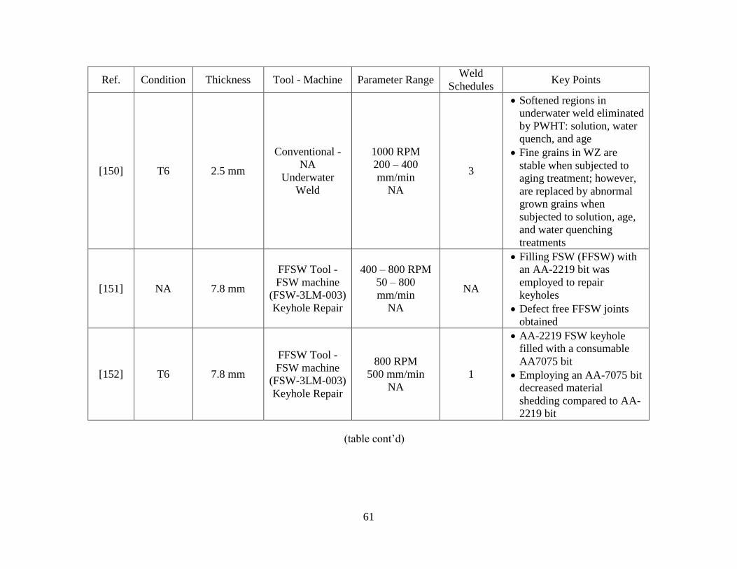
61



[150] T6 2.5 mm

Conventional -

NA

Underwater

Weld

1000 RPM

200 – 400

mm/min

NA

3

Softened regions in

underwater weld eliminated

by PWHT: solution, water

quench, and age

Fine grains in WZ are

stable when subjected to

aging treatment; however,

are replaced by abnormal

grown grains when

subjected to solution, age,

and water quenching

treatments

[151] NA 7.8 mm

FFSW Tool -

FSW machine

(FSW-3LM-003)

Keyhole Repair

400 – 800 RPM

50 – 800

mm/min

NA

NA

Filling FSW (FFSW) with

an AA-2219 bit was

employed to repair

keyholes

Defect free FFSW joints

obtained

[152] T6 7.8 mm

FFSW Tool -

FSW machine

(FSW-3LM-003)

Keyhole Repair

800 RPM

500 mm/min

NA

1

AA-2219 FSW keyhole

filled with a consumable

AA7075 bit

Employing an AA-7075 bit

decreased material

shedding compared to AA-

2219 bit

(table cont’d)

62



[153] NA 6 mm

FFSW Tool -

NA

Keyhole Repair

800 RPM

100 mm/min

NA

1

Lowest hardness occurred

at TMAZ

Elongation decreased with

increased retraction speed

[154] T6 20 mm

Conventional -

NA

Theta-Phase

Agglomeration

450 RPM

120 mm/min

NA

1 Abnormal coarsening of

Al2Cu particles occur in

overlapping repair welds

[155] T6 20 mm

Conventional -

NA

Theta-Phase

Agglomeration

450 RPM

120 mm/min

NA

1

Largest particle size found

was 150 µm

Abnormal coarsened

particles occur in AS for

FS repair welds

Three formation

mechanisms proposed for

abnormal particle

formation

[156] T6 5 mm

SSFSW/NRS-

FSW -

FSW machine

(FSW-3LM-003)

Shoulder

Modifications

600 – 1000 RPM

100 mm/min

NA

5

Non-rotational shoulder

(NRS-FSW) and small

shoulder FSW (SSFSW)

compared

[19] T6 5 mm

NRS-FSW -

FSW machine

(FSW-3LM-003)

Shoulder

Modifications

800 RPM

50 – 300

mm/min

NA

4

NRS-FSW: effect of

welding speed on

mechanical/microstructural

properties

(table cont’d)

63



[20] T6 5 mm

NRS-FSW -

FSW machine

(FSW-3LM-003)

Shoulder

Modifications

600 – 1000 RPM

100 mm/min

NA

5

NRS-FSW: effect of

rotational speed on

mechanical/microstructural

properties

[21] T6 5 mm

RDR-FSW -

FSW machine

(FSW-3LM-003)

Shoulder

Modification

Shoulder-800

RPM

Pin-800 RPM

150 mm/min

NA

1 Reverse dual-rotation FSW

(RDR-FSW) effect

[157] T6 5 mm

RDR-FSW -

FSW machine

(FSW-3LM-003)

Shoulder

Modifications

Shoulder-800

RPM

Pin-800 RPM

50 - 200 mm/min

NA

4 Reverse dual-rotation FSW

(RDR-FSW): effect of

feedrate

[158] NA 3 mm

The IR-FSW -

FSW machine

(FSW-3LM-003)

Shoulder

Modification

NA NA Effect of a surface

treatment device for In-situ

rolling FSW (IR-FSW)

[159] NA 3 mm

The IR-FSW -

FSW machine

(FSW-3LM-003)

Shoulder

Modification

600 RPM

100 – 500

mm/min

NA

5

IR-FSW improves

mechanical properties of

AA-2219 joints by

reducing residual stress and

distortion

(table cont’d)

64



[160] NA 4.55 mm

Conventional -

NA

FSW

Intersection

800 - 1250 RPM

87 mm/min

NA

2

Double-pass FSW grains

are finer than single-pass

FSW

PWHT causes double-pass

FS weld joints to have

faster abnormal grain

growth

[161] T87 5 mm

Conventional -

Indigenous

designed

machine

Multipass FSP

800 – 1600 RPM

22.2 – 45.6

mm/min

12 kN

5

Multipass FSP refines

CuAl2 particles and

improves corrosion

resistance

[162] T851 9.5 mm

FSSW -

Lagun FTV-1

milling machine

and HAAS

TM1 CNC

milling machine

Spot Welds

1000 – 3000

RPM

NA

NA

NA

Liquation tendencies in

FSSW analyzed

Material removed in FSSW

of AA-2219 increases with

increasing tool rotation

[163] T6 5 mm

RDR-FSW -

FSW machine

(FSW-3LM-003)

Shoulder

Modification

800 RPM

200 mm/min

NA

1

Microstructure comparison

between conventional and

RDR-FSW

Grain size in WZ of RDR-

FSW is smaller than

conventional FSW

[164] T6 5 mm

RDR-FSW -

FSW machine

(FSW-3LM-003)

Shoulder

Modification

800-1000 RPM

150-250 mm/min

NA

15

Based on a Box-Behnken

design, optimization of

weld parameters conducted

Maximum tensile strength

of 357 MPa obtained

65

CHAPTER 6 : FSW DEFECTS AND QUALITY CLASSIFICATION

Science is the systematic classification of experience.

-George Henry Lewes

6.1. Introduction

FSW involves controlling three process variables that dictate the movement of the pin tool.

It is difficult to accurately predict the most favorable process parameters to acquire high quality

defect-free welds for a particular weld configuration. For this reason, this chapter discusses the

impact these parameters have on weld defect formation and weld quality. This in turn initiates the

trek towards understanding the weld configuration utilized in this work.

This chapter depicts the initial 66 weld schedules (i.e. combination of the variations in the

three process parameters) that were completed and illustrates the mechanical properties obtained

from those experiments. This includes the effect the weld schedules have on weld defect formation,

uniaxial transverse tensile strength, toughness, and fracture configuration (i.e. fracture initiation

and fracture surface morphology).

6.2. FSW Process Parameters

The three weld process parameters of spindle rotational speed (𝑁), welding speed (𝑉), and

plunge force (𝐹𝑧) are investigated in this section. All other features including pin tool geometry

and clamping conditions are held constant. Spindle rotational speed is defined as tool revolution

per minute (rpm); feedrate is defined as tool welding speed along the weld seam (mm/min); and

plunge force is defined as the downward vertical force applied to the workpiece (kN). The quality

of a FSW joint depends on several factors including tool design, welding parameters, clamp design,

and materials to be welded. This is illustrated in Figure 6-1. For a particular welding condition,

the geometry of the pin tool and weld process parameters play important roles in material

deformation. To produce a high quality defect-free weld, the welding process parameters and pin

66

tool design must be chosen carefully [49, 165-168]. Researchers have studied the effect of different

pin tool geometries and found that tapered threaded pin tools can produce better quality joints

[109, 169, 170]. In this current investigation, a threaded pin tool was utilized.

Figure 6-1 : Line diagram showing factors that affect the quality of a FSW joint.

In the following sections, the impact the process parameters have on the joint quality are

discussed with respect to defect formation, microstructure, and fracture surfaces. The weld

schedules completed that are analyzed in this chapter can be observed in Appendix Table A-1.

6.3. Microstructure of FSW Joints

Microscopic analysis is important to understand weld quality of a FSW joint. Unlike

conventional welding process, the two sides of the FS welded plates are not symmetric. These two

sides are considered the AS and RS as discussed in Chapter 2. In general, a FSW joint is composed

of four distinct regions including the stir zone (SZ) or weld nugget (WN), thermo-mechanically

affected zone (TMAZ), heat affected zone (HAZ), and base metal (Figure 6-2). In Figure 6-2, an

optical macrograph from a polished and chemically etched FSW specimen reveals the four distinct

regions as discussed above. The dotted lines (red, purple, and black) are drawn schematically to

distinguish the SZ, TMAZ, HAZ, and base metal area. A more in-depth view of a FS weld can be

67

observed in Figure 6-3 where transverse optical micrographs of the joint at different locations are

observed.

Figure 6-2: Cross-sectional view of FS welded joint. A FSW joint is composed of SZ, TMAZ,

HAZ, and base metal.

Figure 6-3: Optical micrographs of a defect-free FS welded AA-2219 joint. Micrographs are

taken at different locations showing variations in microstructure.

Figure 6-4 illustrates plan view microstructures and clearly indicates the banding texture

that is observed in FSW. Most of the deformed material is extruded past the RS of the tool and

results in an asymmetrical weld joint [33]. From near-weld and TMAZ interface, evidence of

plastic deformation can be seen in the grain structures. In the outer part of the TMAZ, deformed

grain structure with the formation of sub-grain structures are seen. In the SZ, higher strains and

68

temperatures allowed the formation of the recrystallized nugget with a fine equiaxed structure. In

general, the nugget is comprised of recrystallized grains, whereas, the TMAZ comprises of

deformed sub-grains separated by low angle grain boundaries [171]. The microstructure of the AS

is characterized by a sharp boundary between the SZ and TMAZ. On the RS, the FSW joint has a

more complex microstructure with no clear boundary between the SZ and TMAZ as observed in

Figure 6-4. In Figure 6-5, a plan view image is provided illustrating workpiece material before it

is consumed in the rotating plug of material.

Figure 6-4: Midsectional plan-view of macro- and microstructure created by the FSW pin, tool

spindle rotating clockwise at 400 RPM with feedrate of 4 IPM and plunge force 4000 lbf in 0.32

inches thick AA2219-T87. A closer inspection of the sir zone interface on the AS and RS is

observed in A and B respectively. The microstructure of the stir zone illustrating the material

flow pattern on the AS and RS is observed in C and D respectively.

69

Figure 6-5: Top surface plan-view of macro- and microstructure created by the FSW tool

shoulder and pin, tool spindle rotating clockwise at 400 RPM, feedrate of 4 IPM and plunge

force 4000 lbf in 0.32 inches thick AA2219-T87. Note the consumption of the workpieces’ joint

centerline.

To further the investigation of grain size at different regions, SEM micrographs were

analyzed (Figure 6-6). It observed that the SZ is invariably composed of equiaxed grains with

an average grain size of 5 µm. A clear boundary between weld nugget and TMAZ can easily

be identified at the AS; but in the RS it was not easy to identify the clear boundary between

the SZ and TMAZ which is confirmed from the optical micrographs (Figure 6-3) and electron

backscatter diffraction (EBSD) (Figure 6-7).

Figure 6-6: SEM micrographs of a defect-free FS welded AA-2219-T87 joint. Micrographs are

taken at different locations in the weld showing variations in microstructure.

70

Figure 6-7: Electron backscatter diffraction (EBSD) images of FS welded AA-2xxx (Image

Courtesy: Oxford-EBSD).

6.4. Weld Defect Classification

The quality of a FS weld is largely dependent on heat generated (Q) during the welding

process. For a particular pin tool and clamping condition, “Q” mainly depends on the spindle

rotational speed and feedrate. This topic will be discussed in more detail in Chapter 9. In general,

for a particular combination of spindle rotational speed and feedrate a specific weld temperature

will be realized under steady-state conditions. The plunge force acts as the mechanism which

dictates whether defects will form. Plunge force reduces the tendency for internal surfaces to open

and pushes the crown surface down to maintain full pin length and prevent incomplete penetration

(IP). Hence, all three process parameters in tandem will determine when a defect will form.

Excessive plunge force tends to promote small voids and underfill/flash (UF/F), whereas

insufficient plunge force promotes wormholes (WH), i.e. internal cavities, Trenching (TR) or

surface cavities, and IP. Microscopic analysis and NDT of the FS welded AA-2219-T87 panels

with the 66 different schedules revealed welding defects for 32 schedules leaving 34 defect-free.

Three weld categories were distinguished based on the observed weld defects. These include (i)

hot weld (high spindle speed, low feedrate, and high plunge force), (ii) cold weld (low spindle

speed, high feedrate, and low plunge force), and (iii) nominal weld (optimum spindle rotational

speed, feedrate, and plunge force) as seen in Figure 6-8. Nominal welds were observed to have no

visible weld defects.

71

Figure 6-8 : General classification of welds utilized in this work.

6.4.1 Microscopic Analysis to Classify Weld Defects

In cold welds, the defects observed include WH, IP, and TR. WHs were observed inside

the SZ on the AS of the nugget and IP on the original seam line below the nugget as shown in

Figure 6-9. The IP defect presumably occurs when the tool shoulder rides higher on colder and

harder metal, forcing the pin away from the root side of the weld panel. A cold weld schedule also

produced surface cavities on the AS. The TR surface appears much like the WH surface except

that TR surfaces open to the weld crown surface.

Optical macro- and micrographs illustrating underfill and micro-voids in hot welds can be

seen in Figure 6-10. The shape of the observed IVs were found to be more “penny-shaped” than

round like a gas pore, and their internal surfaces exhibited relatively smooth un-dimpled expanses

that suggest poorly bonded regions inside the SZ [172]. Close to the free surface of the weld crown,

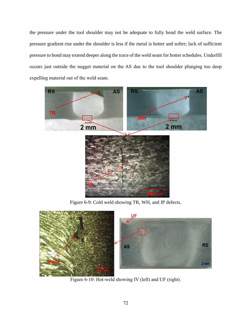
72

the pressure under the tool shoulder may not be adequate to fully bond the weld surface. The

pressure gradient rise under the shoulder is less if the metal is hotter and softer; lack of sufficient

pressure to bond may extend deeper along the trace of the weld seam for hotter schedules. Underfill

occurs just outside the nugget material on the AS due to the tool shoulder plunging too deep

expelling material out of the weld seam.

Figure 6-9: Cold weld showing TR, WH, and IP defects.

Figure 6-10: Hot-weld showing IV (left) and UF (right).

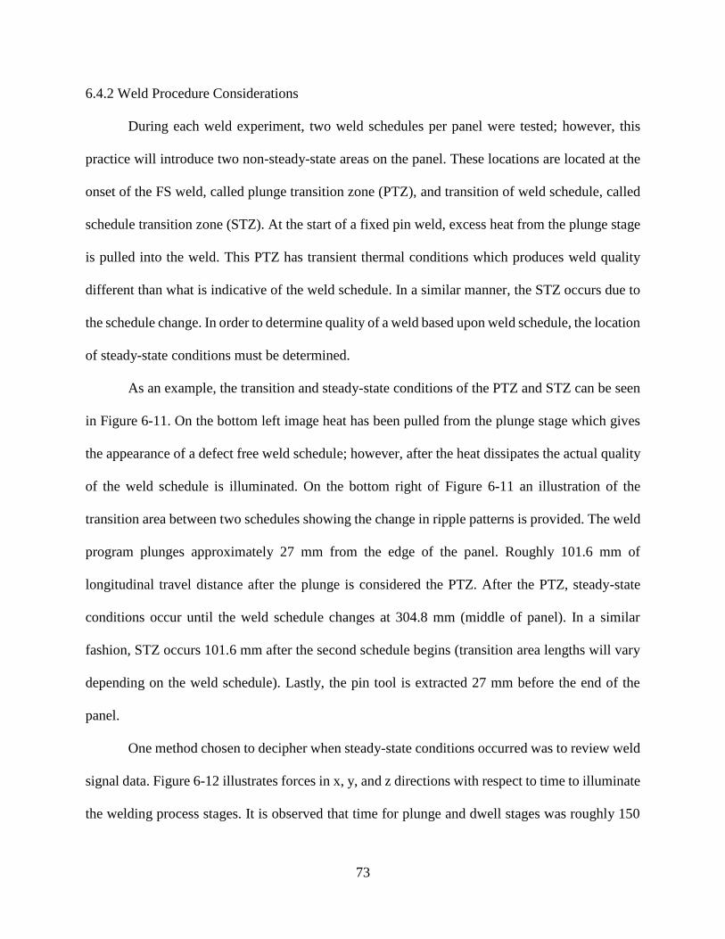
73

6.4.2 Weld Procedure Considerations

During each weld experiment, two weld schedules per panel were tested; however, this

practice will introduce two non-steady-state areas on the panel. These locations are located at the

onset of the FS weld, called plunge transition zone (PTZ), and transition of weld schedule, called

schedule transition zone (STZ). At the start of a fixed pin weld, excess heat from the plunge stage

is pulled into the weld. This PTZ has transient thermal conditions which produces weld quality

different than what is indicative of the weld schedule. In a similar manner, the STZ occurs due to

the schedule change. In order to determine quality of a weld based upon weld schedule, the location

of steady-state conditions must be determined.

As an example, the transition and steady-state conditions of the PTZ and STZ can be seen

in Figure 6-11. On the bottom left image heat has been pulled from the plunge stage which gives

the appearance of a defect free weld schedule; however, after the heat dissipates the actual quality

of the weld schedule is illuminated. On the bottom right of Figure 6-11 an illustration of the

transition area between two schedules showing the change in ripple patterns is provided. The weld

program plunges approximately 27 mm from the edge of the panel. Roughly 101.6 mm of

longitudinal travel distance after the plunge is considered the PTZ. After the PTZ, steady-state

conditions occur until the weld schedule changes at 304.8 mm (middle of panel). In a similar

fashion, STZ occurs 101.6 mm after the second schedule begins (transition area lengths will vary

depending on the weld schedule). Lastly, the pin tool is extracted 27 mm before the end of the

panel.

One method chosen to decipher when steady-state conditions occurred was to review weld

signal data. Figure 6-12 illustrates forces in x, y, and z directions with respect to time to illuminate

the welding process stages. It is observed that time for plunge and dwell stages was roughly 150

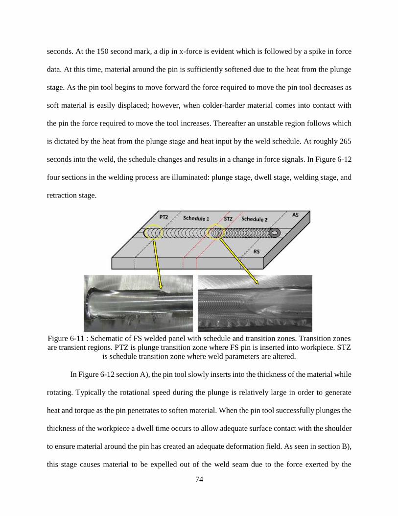
74

seconds. At the 150 second mark, a dip in x-force is evident which is followed by a spike in force

data. At this time, material around the pin is sufficiently softened due to the heat from the plunge

stage. As the pin tool begins to move forward the force required to move the pin tool decreases as

soft material is easily displaced; however, when colder-harder material comes into contact with

the pin the force required to move the tool increases. Thereafter an unstable region follows which

is dictated by the heat from the plunge stage and heat input by the weld schedule. At roughly 265

seconds into the weld, the schedule changes and results in a change in force signals. In Figure 6-12

four sections in the welding process are illuminated: plunge stage, dwell stage, welding stage, and

retraction stage.

Figure 6-11 : Schematic of FS welded panel with schedule and transition zones. Transition zones

are transient regions. PTZ is plunge transition zone where FS pin is inserted into workpiece. STZ

is schedule transition zone where weld parameters are altered.

In Figure 6-12 section A), the pin tool slowly inserts into the thickness of the material while

rotating. Typically the rotational speed during the plunge is relatively large in order to generate

heat and torque as the pin penetrates to soften material. When the pin tool successfully plunges the

thickness of the workpiece a dwell time occurs to allow adequate surface contact with the shoulder

to ensure material around the pin has created an adequate deformation field. As seen in section B),

this stage causes material to be expelled out of the weld seam due to the force exerted by the

75

shoulder. Typically, the area where plunge and dwell stage occurred is left with a surface cavity

due to a lack of material to be welded as material was expelled in this area. Section C) illustrates

the region where welding occurs. This region is the location where weld coupons were taken.

Lastly, section D) provides the end of the weld with retraction of pin tool.

Figure 6-12 : Force profiles vs. time (signal data acquisition rate 60 Hz). Schedule 1 [200 RPM -

152.4 mm/min - 33.36 kN]; Schedule 2 [450 RPM - 152.4 mm/min - 33.36 kN]. Below are weld

stage images corresponding to force data: A) Initial plunge stage, B) Dwell stage before pin tool

begins to travel, C) Welding stage, D) Retraction stage.

Defect classification must be carefully evaluated because defects form due to different

mechanisms. Therefore, an initial classification of defects was made based upon size, shape, and

location. In Figure 6-13, optical micrographs and SEM images of a defect and defect free specimen

are observed. The optical micrographs illustrate cross-sectional images of the FS welded

specimens whereas SEM images show fracture surfaces of tensile tested specimens. It is observed

that the ‘onion-ring structure’ [173] in the defect free weld is consistent with no abrupt changes,

76

which is conducive to high strength mechanical properties. In the WH defect specimen, it is

observed that the onion pattern appears to have similar characteristics as the defect free specimen

on the RS; however, on the AS the onion pattern abruptly changes as it approaches the defect. It

is observed that the onion patterns appear as if it was squeezed compared to the larger separation

on the RS.

Figure 6-13 : Optical micrographs of cross-section and fracture specimen of a defect free and

defective specimen with WH and IP. SEM images illustrate large fracture dimples indicating

larger grains outside of SZ and internal structure of wormhole defect showing regions of bonded

(dimples) and un-bonded (surface ripples) material.

77

Fracture in the defect free specimen occurred on the RS. The WZ is stronger than the HAZ

and TMAZ as the microstructure has fine-equiaxed grains compared to larger coarsened grains.

Large grains allow fracture propagation and are the weakest region in the weld. It is observed in

the SEM image that large fracture dimples occur which indicates larger coarsened grains away

from the WZ. Alternatively, the defect specimen incurred fracture which initiated at the root of the

weld due to an IP defect. The fracture propagated through the WZ to the weakest point at the edges

of the WH defect. SEM images illuminate the internal structure of the WH defect. It is observed

that material flow patterns resemble ripple patterns on the top surface of a FS weld. The shiny

smooth surface indicates non-bonded material whereas darker areas indicate fracture dimples of

once bonded material.

6.5. Tensile Properties of FS Welds

Uniaxial ultimate tensile strength (UTS) and toughness have been investigated to

understand the effects of varying weld schedules. Tensile tests were conducted along the transverse

direction of the weld seam. These results can be seen in Appendix Table A-1. Typical tensile stress-

strain curves for base metal, nominal, hot, and cold welds are shown in Figure 6-14 below. Defect-

free nominal welds exhibited UTS and toughness values equal or more than 66% and 43% of base

metal values.

The variation in tensile strength and toughness values of nominal, hot, and cold welds are

related to weld defects and microstructure. Typical SZ microstructures of nominal, hot, and cold

welds are shown in Figure 6-15. The grain growth in the SZ is related to heat input during the

welding process [110]. The weld nugget of a defect free FSW joint is commonly composed of fine

equiaxed grains (Figure 6-15a). The high heat input in hot welds resulted in growth of the

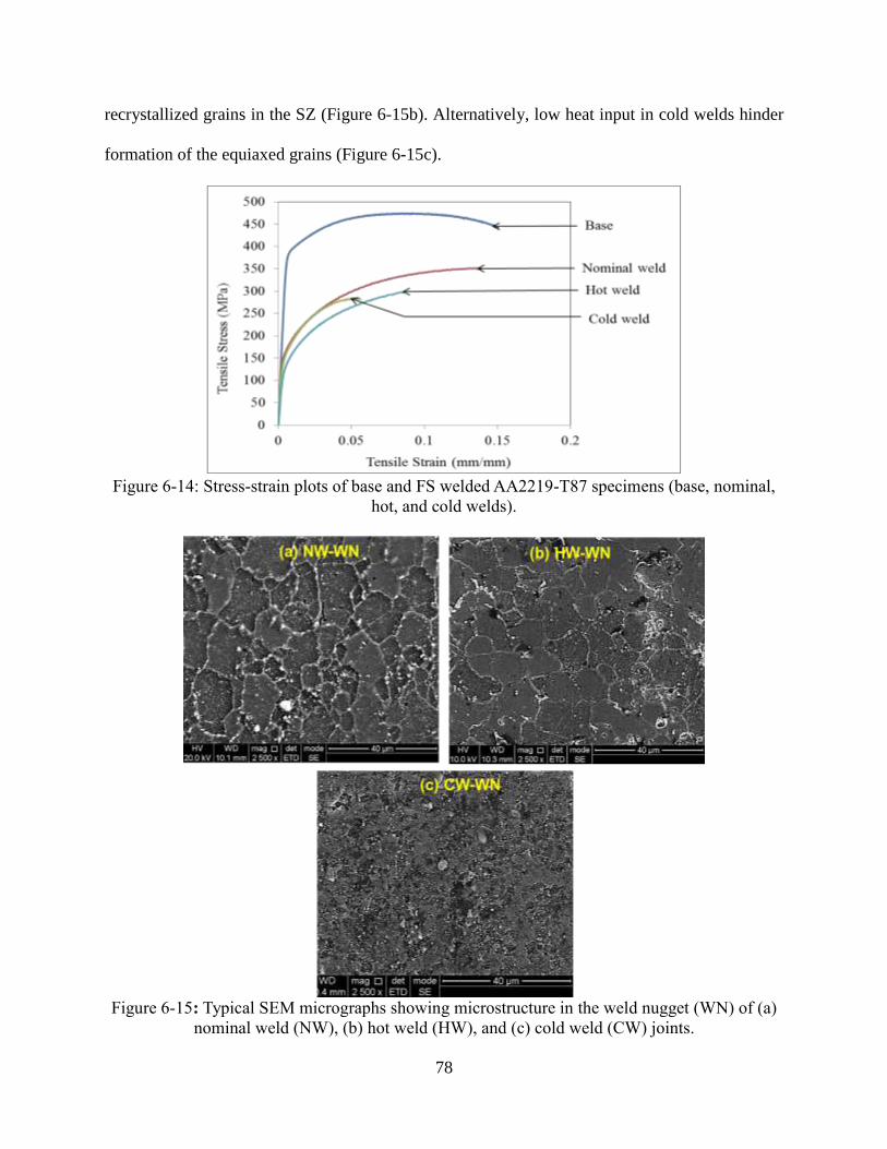
78

recrystallized grains in the SZ (Figure 6-15b). Alternatively, low heat input in cold welds hinder

formation of the equiaxed grains (Figure 6-15c).

Figure 6-14: Stress-strain plots of base and FS welded AA2219-T87 specimens (base, nominal,

hot, and cold welds).

Figure 6-15: Typical SEM micrographs showing microstructure in the weld nugget (WN) of (a)

nominal weld (NW), (b) hot weld (HW), and (c) cold weld (CW) joints.

79

Both UTS and toughness values of welded specimens decreased with the increase of defect

size. Nominal welds were observed to have the highest average UTS (332 MPa) and toughness (37

MJ/m³) values, followed by hot welds with underfill (311 MPa and 24 MJ/m³), cold welds with IP

(271 MPa and 15 MJ/m³), cold welds with WH (273 MPa and 10 MJ/m³), and cold welds with TR

(170 MPa and 5 MJ/m³). The following Figure 6-16 illustrates the variation of UTS and toughness

values with different defect types.

Figure 6-16: Effect of different weld defects on tensile properties (NW: nominal weld; HW: hot

weld; CW-IP: cold weld with incomplete penetration; CW-WH: cold weld with wormhole; CW

TR: cold weld with trenching).

6.6. Fracture Surface Analysis

The following Figure 6-17 - Figure 6-20 show fracture surfaces and related microstructural

features of tensile tested samples of nominal, hot, and cold welds. A fracture surface of a nominal

weld with no-defects is shown in Figure 6-17. Fracture occurred on the 45o maximum shear line

in the HAZ outside the weld nugget on the RS of the weld. Beyond the nugget in the TMAZ and

HAZ the softening effect of over-aging [174] predominates and presents a path for fracture. The

80

fracture surface exhibits ductile rupture dimples [48] of a larger size corresponding to the larger

parent metal grains outside the nugget zone.

Figure 6-17: Nominal weld showing no defect. A 45° maximum shear fracture is on retreating

side of tool outside the weld nugget in heat-affected base metal. Fracture surface exhibits ductile

fracture dimples, larger corresponding to base metal and weld nugget.

The following Figure 6-18 illustrates optical images and fracture surfaces of a tensile tested

hot weld specimen. All hot welds, based upon the classification, have UF on the AS of the SZ. In

some cases, internal voids were present within the nugget metal on the AS as discussed previously.

The voids might be entrained from a free surface by ring vortex circulations and un-bonded regions

on the weld seam trace. Close to the free surface of the weld crown, the pressure under the tool

shoulder may not be adequate to fully bond the weld surface. The internal surface of the voids

show patches of ductile fracture dimples, but also smooth surfaces with some regular linear

grooves that suggest ripples produced on an internal un-bonded surface in the same way they are

produced on the crown surface in the wake of the weld. These ripples can be seen at the bottom of

81

a crack in the rippled surface following the tool. The fracture is no longer a shear fracture, but now,

judging by the orientation normal to the test coupon surface, a tensile fracture.

Figure 6-18: Hot weld showing an IV. Fracture is on the AS of the tool inside the SZ. Fracture

surface exhibits equiaxed ductile fracture dimples, smaller corresponding to base material.

Unbonded void surface exhibits some regularly space curved lines that may be internal ripples.

An example of a cold weld schedule that produced a WH and IP on the original seam line

below the weld nugget can be seen in Figure 6-19. The IP presumably occurs when the tool

shoulder rides higher on colder and harder metal, retracting the end of the pin from the root side

of the weld panel. Under load control, colder and harder metal is more difficult to indent because

the pin will be pushed out of the seam and a compensatory increase in plunge force will not occur

which leads to IP. Similar defect types associated with this phenomena can also occur such as the

joint line remnant (JLR), kissing bond (KB), or root flaw. In [175], a KB is defined as a solid-state

welding defect where two pieces of material are in contact but have failed to create any metallic

bonds. It is also reported that the KB originates from insufficient mixing of matter close to the

initial butt surfaces [41, 176]. The cause of JLR defects in FSW have been linked to slipping

82

conditions between the tool surface and metal in the shear zone and oxide layers brought into the

SZ.

The WH in Figure 6-19 exhibits two distinct surfaces: a smooth surface following the

nugget edge on the trace of the shear surface and rounded surfaces incorporating ripples that appear

on the free surface trailing the weld shoulder. The surfaces are separated by cusps. Above and

below the WH defect the fracture surface exhibits ductile rupture dimples. The streamlines of

weld metal flow [177] past the upper portion of the pin does not get close enough to the pin for the

threads to produce an impression on the weld metal. The pumping action on the weld metal due to

slight eccentricity of the rotating pin tool is responsible for the ripples in the wake of the weld as

well as internal bonding texture and ripples on any internal open surface. Both apparently un-

bonded clean ripples and adjacent periodic bonded dimpled surfaces that appear to be banding

texture are visible in SEM fractographs. The fracture surface follows a less defined 45o line through

a defect and along a direction suggesting minimal shear strength.

Figure 6-19: Cold weld showing internal cavity. Fracture is on the AS of tool inside the weld

nugget. Fracture surface exhibits ductile fracture dimples, smaller corresponding to nugget

material. Unbonded cavity surface appears to exhibit surface ripples.

83

The cold weld also exhibits TR with ripples on the trench surface (Figure 6-20). The

internal cavity on the AS of the cold weld has enlarged and moved to the surface. The fracture

surface is almost at 45o implying a shear mechanism. With colder, harder metal under load control

the shoulder may not press as deeply into the metal so that the effective pin depth is reduced. As a

result the IP at the weld root is more pronounced, as anticipated, for load control operation.

Figure 6-20: Cold weld showing TR defect at weld crown and IP at weld root. Fracture is on AS

of tool inside the weld nugget. Fracture surface exhibits ductile fracture dimples, smaller

corresponding to nugget material. Unbonded trench surface exhibits surface ripples.

6.7. Micro-Hardness of FS Welds

To understand the fracture behavior of nominal, cold, and hot weld joints hardness profiles

were investigated. Rockwell hardness values (60-kgf, diamond cone, HRA scale) are measured at

the middle of the cross section of the FSW joint. The measured hardness profile is plotted against

distance from weld centerline, and an example can be seen in Figure 6-21. The SZ exhibited higher

hardness values compared to AS and RS TMAZ. Higher hardness values at the SZ is related to the

equiaxed fine grain structure. A lower hardness value near TMAZ is related to deformed and

elongated microstructure. The lowest hardness value (about 24 HRA) is exhibited near the TMAZ

on the RS which correlates with optical micrographs. It is observed in this study that differences

84

in hardness values at AS and RS is not significant to dictate failure sites in defective joints in the

case of tensile tests.

Figure 6-21: (a) Cross sectional view and (b) Micro-hardness profile of FS- welded AA2219-T87

joint.

6.8. Summary

The FSW process can generate defects if not correctly designed. For a particular pin tool

and welding condition, the quality of a FS weld greatly depends on three process parameters

including plunge force, spindle rotational speed, and feedrate. To understand the effects of varying

welding process parameters, the weld schedules were classified into three general categories of

hot, nominal, and cold welds. The presence of defects reduces mechanical properties, especially

ultimate tensile strength and toughness values. The defects that were observed from this study

include WH, TR, IP, UF/F, and IV. Welds were characterized based upon their hardness, tensile

strength, observable defects, and optical techniques. In the following chapter, information gained

from this study will be employed to create a process parameter window of the FSW configuration.

85

CHAPTER 7 : DEVELOPMENT OF A NEW PROCESS PARAMETER

METHODOLOGY AND EMPIRICAL FORCE INDEX TO DETERMINE

WELD QUALITY

Without continual growth and progress, such words as improvement, achievement, and success

have no meaning.

-Benjamin Franklin

7.1. Introduction

In the previous chapter, knowledge gained from experimental mechanical testing of the

FSW configuration was presented. It was shown that for a particular FSW pin tool and clamping

condition the quality of a FS weld largely depends on the three process parameters of spindle

rotational speed, feedrate, and plunge force. Theoretical indices (i.e. combination of critical

process parameters) have been suggested in the literature to realize the impact that these process

parameters have on joint quality; however, in most cases these indices neglect plunge force. An

ideal index would be one that determines how all three parameters can be varied together to obtain

weld quality. Additionally, a more powerful theoretical aid would be a defect formation criterion

or a parametric relationship establishing the boundary between welds with a particular defect and

welds without a defect.

Often in the literature the spindle rotational speed and feedrate are varied, and in most cases

with position-control. In position-control the pin tool will remain at a certain target depth which

will cause variations in plunge force values to hold the pin at the target depth. This variation will

cause fluctuations that can create variation in weld quality and produce non-consistent mechanical

properties. On the other hand, load-control can provide more consistent results as the plunge force

is constant; however, if the plunge force is not adequate then defects can form. In either control

setting the process parameters are often represented in a 2-dimensional plot identifying the weld

quality. Typically in research and development a trial and error method is used to determine

86

appropriate welding operating windows. In general, for a certain welding condition a range of

operating conditions (spindle rotation speed and feedrate) are available for a particular plunge

force. At select plunge forces the range of spindle rotational speed and feedrate leading to defect

free welds can be maximized. These process parameter maps can be created by taking a slice from

this three-dimensional process parameter field to create a two-dimensional map as seen in [94,

120, 178-180].

The current study aims to develop such an empirical relation and process parameter

methodology which identifies information about defect formation mechanisms that may be

applicable to a more general understanding of what determines the operational parameter window

for FSW. In the subsequent sections, the relationships between feedrate and spindle rotational

speed are analyzed identifying the various process parameter indexes. Consequently, development

of an empirical relationship that can aid in predicting weld quality is presented and compared to

what is found in the literature. Additionally, development of a new process parameter window

methodology that represents the three FSW process parameters into a 2-imensional plot is

presented. The work in this chapter aims to provide a better methodology for choosing process

parameters for weld development which can help decrease cost and time.

7.2. Development of the Pin Speed Ratio

7.2.1. Indexes Observed in the Literature

Works in the literature that have suggested indexes are analyzed in this section. Firstly, an

empirical Pseudo Heat Index (PHI) has been proposed by Kandukuri and his research group [181]

to correlate the heat input during FSW with spindle rotational speed and welding speed. If heat

input determines weld properties, similar welds are obtained by holding the index constant. The

PHI does not include many process features affecting weld properties and is only good for a certain

87

range of feedrate and spindle rotational speed for a specified welding situation. Nunes [182] has

proposed a temperature index based on a physical model of the FSW process in which temperature

is computed from a heat balance relationship. In that model, shear stress is assumed to be linearly

related to temperature. Another research group [183] has proposed an Alternative Heat Index

(AHI) considering heat generation and thermal dissipation. A linear approximation was used to

capture thermal softening with temperature; however, flow stress may not be linearly related with

temperature. Dehghani and other researchers [184] suggested a Heat Input Factor (HIF) to

determine weld quality. In their model plunge force is assumed constant and feedrate has a linear

relation with weld heat generation. None of these indices included plunge force, yet plunge force

is a key parameter that impacts the formation of defects.

The indexes discussed above were tested against data obtained in this study. In [184-186]

the suggested energy input model assumed heat input is related to torque, spindle rotational speed,

and welding speed. Heat input per unit length can thus be expressed as Eq. (7.1).

𝐸𝑛𝑒𝑟𝑔𝑦 𝐼𝑛𝑝𝑢𝑡 (𝐸𝐼) = 𝑇𝑜𝑟𝑞𝑢𝑒 × 𝑁

𝑉 (7.1)

In Figure 7-1a, UTS values are plotted against energy input and failed to separate classifications

used in this study (nominal, cold, and hot welds). In their model, plunge force is assumed to be

constant and feedrate having a linear relation with welding heat generation. Kandukuri and his

research group [181] proposed the empirical PHI to correlate the heat input during FSW with

spindle speed and welding speed. If heat input determines weld properties, similar welds are

obtained by holding the index constant. The PHI can be expressed as Eq. (7.2).

𝑃𝐻𝐼 =

𝑁

(10,000 × 𝑉)

(7.2)

88

In Figure 7-1b, PHI vs. UTS value are plotted, and it is seen that it failed to separate nominal, cold,

and hot weld schedules. Querin and Schneider [183] proposed an Alternative Heat Indexing (AHI)

equation considering heat generation terms and thermal dissipation, as seen in Eq. (7.3).

𝐴𝐻𝐼 =

𝑇 − 𝑇0𝜏

= 𝐴 𝑁

𝐵 + 𝑉

(7.3)

A and B are constants related to material properties, heat transfer coefficients, and pin tool

geometry. In Figure 7-1c, experimental UTS values are plotted against AHI. The AHI did not

include plunge force, and also failed to determine the three ranges of weld quality in this study.

Figure 7-1: Experimental ultimate tensile strength (UTS) values are plotted against (a) energy

input, (b) Pseudo heat index, and c)Alternative heat index.

In FSW, the spindle speed (𝑁) and feedrate (𝑉) have opposite consequences on frictional

heat generation [167]. It is the author’s belief that a better way to represent welding process

parameters in a more concise manner can be achieved by combining 𝑁 and 𝑉 together for the

89

purpose of creating a 2-D plot to represent weld schedules. It can be seen in Figure 7-2 that with

5 similar spindle rotation speed and feedrate values but varying plunge force optimum tensile

properties vary. In these welds, the quality of the weld is consistent through the entire length as

observed by destructive testing and tool force examination. It is seen that with an increase in plunge

force tensile properties increase to a maximum which then begin to drop. These curves are directly

related to process parameters which allow formation of defects due to heat input and material

rupture suppression of the weld system. It is noted that in Figure 7-2 a sharp increase in toughness

is evident. For these welds defects have occurred due to an indecorous welding environment

leading to defects (left hand side of maximum toughness value). With an increase in plunge force

favorable conditions are present allowing plastic flow of material to successfully form metallic

bonds. As the plunge force is further increased an excess of force allows the shoulder of the pin

tool to sink causing flash and underfill defects as the welding material becomes excessively

softened. It can be seen in Figure 7-2 that tensile properties on the right hand side do not have as

sharp a gradient as seen on the left hand side due to the different defect mechanisms associated

with the process parameters.

Process parameters are directly related to the material flow. In [187] material flow during

FSW is analyzed providing insight into the shearing of material due to pin tool movement. The

deformation of material has been analyzed in [33, 47, 188-190] as well. The material flow has been

modeled in [191] with three incompressible flow fields. Consequently, two parameters cannot

accurately determine the quality of a weld and does not adequately demonstrate the cause for defect

formation. Conclusions cannot necessarily be made by neglecting the plunge force or its effects if

one is comparing quality, as position-control will vary the plunge force automatically. If position-

control is used, an increase in rotational speed or decrease in feedrate will cause plunge force to

90

decrease in order to obtain a constant pin depth. Moreover, in position control, a battle with heat

input causes variation in the plunge force to keep the pin at the target depth and likewise will cause

tool forces to have large fluctuations.

Figure 7-2 : Effect of plunge force on tensile strength and toughness at constant rotation.

Hence, a dimensionless speed ratio (R) has been proposed as a function of 𝑁 and 𝑉 for

correlating with plunge force (𝐹𝑧). To obtain a dimensionless speed ratio, 𝑁 was multiplied with

the circumference of the pin tool (2𝜋𝑟) and divided with V. The dimensionless speed ratio (𝑅) is

expressed in Eq. (7.4). Here, r is the pin radius.

𝑅 =

2𝜋𝑟𝑁

𝑉

(7.4)

Employing this correlation of weld process parameters, weld quality can be determined by

plotting speed ratio (𝑅) vs. UTS and toughness as seen in

Figure 7-3 (Fz = 22.25 𝑘𝑁 𝑎𝑛𝑑 Fz = 26.69 𝑘𝑁). Trends emerge indicating when plunge force

increases a lower speed ratio is required to obtain better tensile strength and toughness. Higher

plunge force values also reduce the speed ratio window to obtain defect free nominal welds with

high tensile properties. As the speed ratio is increased, a peak value indicating a nominal weld

91

occurs; thereafter, as the speed ratio (𝑅) increases hot welds form. The spindle rotational speed

generates frictional heat as well as stirs and mixes plasticized material around the pin tool [16].

The feedrate prompts the translation of material from the front of the pin tool to the back. The

rubbing of tool shoulder and pin with the workpiece generates frictional heat; consequently, the

feedrate determines the exposure time of this frictional heat per unit length of weld [192]. All other

things being equal, slower feedrate leads to higher heat generation causing improper consolidation

of stirred material. On the other hand, higher feedrate causes lower heat generation and stirring of

plasticized material becomes insufficient. Thus, the material present in the AS of the tool does not

travel through to the RS [193]. Lower spindle rotational speed (𝑁) causes lower heat generation

and lack of stirring around the weld nugget. The net result is poor consolidation of material which

leads to poor UTS and toughness.

Figure 7-3: Effect of speed ratio (𝑅) on (a) UTS and (b) Toughness at constant plunge force (Fz).

In Figure 7-4, plunge force vs. UTS and Toughness have been plotted at two different speed

ratios (R). As the plunge force increases, tensile strength and toughness values increase; thereafter

both strength and toughness values begin to decrease. The reasons UTS and toughness values are

low at the left and right portions of the plot are due to defects that have formed. Heat generated by

92

weld metal deformation around the pin tool softens the weld metal and reduces the axial force

required to indent the weld metal. Axial force also extends the plunge depth of the pin [194, 195].

For a FS weld, the pressure across the weld seam must be high enough to push down asperities

(several times the flow stress of the material) for joining to occur. Lower heat generation causes

higher flow stress and hence weld defects due to improper consolidation of material [196] and

results in lower tensile strength. Higher plunge force remedies the effects of colder welds but

excessive plunge force causes deeper tool shoulder penetration depth which causes flash

generation, local thinning (underfill) of the welded plate and reduced tensile strength. Optimum

plunge force is required for avoidance of cold and hot defects and production of sound weld joints.

The speed ratio determines optimum plunge force. At lower speed ratios higher plunge force is

required to obtain nominal welds.

Figure 7-4: Effect of plunge force (Fz) on (a) ultimate tensile strength (UTS) and (b) Toughness

at two different speed ratio (R).

To verify the effect of the dimensionless speed ratio (R), six weld schedules were

conducted at three different speed ratios (Table 7-1). For a particular plunge force two welds were

conducted by varying rotational and feedrate while the speed ratio remained constant. The results

indicate that at a constant speed ratio similar weld quality can be obtained. However, there is a

93

difference in UTS and toughness values observed between two schedules which are still in the

error limit.

By observing characteristic defect types identifiable by non-destructive evaluation of RT

and PAUT as well as metallographic procedures, the schedule-based classification of FS welds as

nominal, hot, and cold welds can be expanded to include not just weld spindle rotational speed and

feedrate, but also plunge force. The characteristic of no-defect microstructure of a nominal weld

which is a category between hot and cold weld, and can be obtained for a wide range of speed

ratios by altering plunge force. At lower speed ratios, higher plunge is required to obtain nominal

welds while lower plunge force is required for higher speed ratios.

Table 7-1 : Verification of the effect of speed ratio (R).

N

[RPM]

V

[mm/min]

Fz

[kN]

Dimensionless

Speed Ratio, R

UTS

[MPa]

Toughness

[MJ/m³] Defect

350 237.0 26.7 47.1 359.96 38.57 None

300 203.2 26.7 47.1 318.59 27.52 None

300 76.2 17.8 125.6 320.65 31.23 None

400 101.6 17.8 125.6 337.37 37.8 None

350 266.7 30.2 41.9 356.56 41.78 None

300 228.6 30.2 41.9 326.33 39.64 None

7.3. Process Parameter Window

A FSW experimental setup for a particular tool-workpiece combination can be conducted

with a certain range of process parameters among which three regions can be generally defined:

region of unstable welding (due to excessive heat input), region of sound welding (as a result of

adequate heat input), and region where unsatisfactory consolidation of material similar to milling

(due to lack of heat input). Defects that reduce the strength of welds are produced with many

parametric conditions. Between conditions that produce defects, it appears in our own studies as

well as those studies of which we are aware that FS welds show little variation in strength. Outside

this process parameter “window” the weld strength drops markedly. Manufacturers operate within

94

this process parameter window. The parameter establishment phase of a welding operation

constitutes the establishment of this process parameter window. Different process parameter

windows may need to be established for different metals and thicknesses, different tool shapes,

perhaps even different machines. Substantial resources are expended in the determination of

process parameter windows and they are generally kept as proprietary information not available to

the public.

Lakshminarayanan et al. [94] discussed improving trial and error methodologies for

selecting process parameters. A processing window was determined by varying feedrate and

spindle rotational speed and reviewing macrostructural or visible defects. At a plunge force of 12

kN, a range of feedrates and spindle rotational speeds with 22 different weld schedules were

conducted. In their study, one operating window at one plunge force was evaluated. Consequently,

the ranges of various regions when defect and non-defect welds occur were determined.

Comparing to our study, we have analyzed a larger range of operating conditions with varying

plunge forces. Furthermore, we attempted to stay within the operating window of our pin tool,

which in their study appear to weld with process parameters outside the acceptable pin tool range.

In reality, process parameter ranges require three parameters in a 3-dimensional operating

space. The operating window within the 3-D space will vary if one or more of the FSW

configurations are changed. It has been presented in literature, as seen Section 7.1, that a two-

dimensional map is applicable only for one plunge force value; consequently, these two-

dimensional maps do not reveal the entire picture of the operating range. In order to group all three

weld parameters, and to illuminate the process parameter window at multiple plunge forces a new

representation was devised. Employing the pin speed ratio (R) as seen above, the three process

parameters can be superimposed into a two-dimensional plane as seen in Figure 7-5. Grouping

95

defects with a general classification of hot, cold, and nominal provides distinct trends. Employing

this general classification, it is observed that a distinct non-linear defect free region (nominal) is

formed.

As seen in ref. [94], a relatively low plunge force was utilized and was stated to be the

acceptable range for their configuration. Another study, Balaji et al. [95], aimed to determine

optimum welding conditions employing ANOVA and regression analysis. It was determined that

with a welding speed 256.4 mm/min, plunge force of 29.62 kN, and rotational speed of 492.9 RPM

yielded optimized mechanical properties. In other studies very high rotational speeds have been

utilized with low plunge forces. High rotational speeds are required if a low plunge force is

employed. A larger rotational speed, coupled with a decrease in feedrate is needed to generate

sufficient heat so that the pin can plastically deform material and consolidate the weld. Figure 7-5

likewise shows the same trend that as plunge force decreases, the required pin speed ratio will have

to be larger. This correlates to higher rotational speeds or lower feedrates.

Figure 7-5: FSW process parameters for hot, nominal, and cold welds group together into fields

with distinct boundaries.

96

It is observed in literature RPM ranges can exceed pin tool design conditions which is

evident from vast generation of flash. Large flash generation expels material in the welded area

and likewise causes adverse effects which are detrimental to a weld’s quality. On the other hand,

low RPM values can cause other defects which adversely impact the quality of a weld. The

operating window for our pin tool’s rotational speed was found to lie between 200 - 450 RPM. At

the 200 RPM boundary, tool forces greatly increased at low plunge forces. In order to save the pin

from excessive stress, and to prevent breakage, this RPM was deemed the cut-off. At 450 RPM

high plunge forces were required to be employed that caused instability in the plastic flow field

causing what is believed to be “slipping” of material that was once “sticking” to the pin. When

slippage occurs, the material does not entrain itself, or “stick”, with the pin and is left

unconsolidated. When this occurs small defects form which have been deemed internal voids (IV),

and have been located in three weld schedules with a rotational speed of 450 RPM, plunge force

in excess of 28.91 kN, and feedrate of 152.4 mm/min. Figure 7-6 illustrates these defects with

associated phased array ultrasonic testing (PAUT) inspection. The voids occurred in the AS away

from the WZ/TMAZ interface, but formed inside the weld nugget area. Thus, 450 RPM was

deemed the cut-off region so that data could be acquired between the two RPM ranges. Nominal

welds may still be able to be generated at higher RPM values with our configuration; however, as

seen in Figure 7-5, the number of feedrate combinations decrease as the plunge force decreases.

In Figure 7-5 two lines were superimposed to signify the boundaries between the three

weld quality regions. The three classifications are based upon tensile properties and defects

observed. In the center region, defect free welds were obtained. Distinct cut-off boundaries of the

defect free weld regions are hard to establish, especially in the upper bound. Tensile properties are

often similar at this boundary. At these locations on the boundary the only significant variation is

97

the underfill defect which promotes low toughness values. In few cases, the ultimate tensile

strength of these welds exceeded that of the defect free welds. This is important in weld

development as one must determine which mechanical property one wants to optimize. On the

opposite boundary, IP defects defined the boundary when process parameters exceeded nominal

conditions. The lower bound cut-off region is easier to define than the upper bound, as IP defects

are easily characterized during destructive and non-destructive tests. During weld development

this new process parameter window can be employed to determine defect boundaries and provide

a guide to weld quality prediction by process parameter selection. Any schedule within the

bounded field produces defect-free welds.

Figure 7-6 : Internal Void (V) defect macrograph (top left) and micrograph (top right) with

associated PAUT A-Scan (bottom left) and S-Scan (bottom right).

7.4. Empirical Force Index

In Section 7.2., indexes developed in the literature that relate to FSW process parameters

was presented and it was found these did not utilize plunge force. In order to determine parameters

that optimize weld quality, a relation consisting of the three principal weld parameters is developed

98

here. From the 66 weld schedules, 34 schedules are classified as defect-free nominal welds. The

nominal welds exhibited UTS and toughness values equal or more than 66% and 43% respectively

of base metal values. If the nominal welds are plotted alone with the process parameter

methodology in Section 7.3., the defect-free weld trends can be defined as seen in Figure 7-7. It is

also observed that as PSR increases, the plunge force required to achieve nominal welds decreases.

Using a non-linear regression approach a correlation between plunge force and PSR for producing

defect-free nominal welds can be written as seen in Eq. (7.5):

𝐹𝑧 = 𝐶1(𝑃𝑆𝑅)−𝐶2 (7.5)

where, 𝐹𝑧 is the plunge force measured in kN and 𝑃𝑆𝑅 is the dimensionless pin speed ratio. The

constant 𝐶1 and exponent 𝐶2 depend on welding material, pin tool design, and other welding

conditions (e.g., clamping condition, chill bar, backing plate, environmental temperature

conditions, etc.) and can be determined experimentally. For least square curve fitting, the

coefficient 𝐶1 and 𝐶2 can be expressed as:

𝐶2 =

𝑛∑ (𝑙𝑛𝑅𝑖 × 𝑙𝑛𝐹𝑧𝑖) − ∑ (𝑙𝑛𝑅𝑖) × ∑ (𝑙𝑛𝐹𝑧𝑖𝑛𝑖=1 )𝑛

𝑖=1𝑛𝑖=1

𝑛∑ (𝑙𝑛𝑅𝑖)2 − (∑ 𝑙𝑛𝐹𝑧𝑖)

2𝑛𝑖=1

𝑛𝑖=1

(7.6)

𝐶1 = exp (∑ (𝑙𝑛𝐹𝑧𝑖) − 𝐶2∑ (𝑙𝑛𝑅𝑖)

𝑛𝑖=1

𝑛𝑖=1

𝑛) (7.7)

In the current study the values of 𝐶1 and the exponent 𝐶2 are 245.43 and 0.551 respectively.

Once the constants in Eq. (7.5) are established it is possible to correlate the types of defects to be

anticipated (and hence weld quality) with an empirical index as seen in seen in Eq. (7.8). This

index has been coined the “Empirical Force Index” (EFI). When this EFI value deviates from unity

defect free welding conditions are lost.

𝐸𝐹𝐼 =𝐹𝑧𝐶1(𝑃𝑆𝑅)𝐶2 (7.8)

99

For nominal welds, the EFI is approximately 1.00. If the EFI is increased the weld tends to be

within the hot classification range with associated defect characteristics. Alternatively, as the EFI

drops below 1.00 defect characteristics of cold welds are observed. The ranges of the EFI

associated with weld quality (UTS and Toughness) are shown in Figure 7-8a and Figure 7-8b.

Figure 7-7: Plunge force vs. pin speed ratio plotted to obtain empirical correlation among three

weld process parameters for nominal weld.

Figure 7-8: Variations of tensile properties with empirical force index (EFI): (left) Toughness

vs. EFI, and (right) Ultimate tensile strength vs. EFI. Mechanical properties decline on either

side of an EFI of 1.00.

For the defect classification three ranges of EFI values can be expressed:

100

0.68 < 𝐸𝐹𝐼 ≤ 0.96 ; 𝐶𝑜𝑙𝑑 𝑊𝑒𝑙𝑑 (𝑊𝐻, 𝑇𝑅, 𝐼𝑃) (7.9)

0.87 < 𝐸𝐹𝐼 ≤ 1.11 ; 𝑁𝑜𝑚𝑖𝑛𝑎𝑙 𝑊𝑒𝑙𝑑 (𝑁𝑜 𝐷𝑒𝑓𝑒𝑐𝑡𝑠) (7.10)

1.08 < 𝐸𝐹𝐼 ≤ 1.77 ; 𝐻𝑜𝑡 𝑊𝑒𝑙𝑑 (𝑈𝐹/𝐹𝑙𝑎𝑠ℎ, 𝑉𝑜𝑖𝑑𝑠) (7.11)

It is observed there is an overlap in EFI values at the interfaces of each classification. This

is due to the boundary where slight changes in process parameter impact the joint quality. This

region is further discussed in Chapter 8. In order to validate the developed EFI, six weld schedules

were conducted with different weld process parameters. The welded plates were inspected with

PAUT and tensile tested to obtain joint properties and classification. Welding parameters along

with EFI, tensile properties, and quality of the joint are listed in Table 7-2. The EFI predicted weld

classification of these welds exactly matched with the experimental results. Therefore, this

relationship may be utilized for the prediction of weld quality based upon all three process

parameters as long as several data points at various ranges are available. The EFI may help mitigate

the trial-and-error approach of choosing weld schedules and can lead the investigator to zero-in on

a desired weld quality.

Table 7-2: New weld schedules along with weld quality for the validation of developed of

empirical force index (EFI) in weld classification. (NW – Nominal Weld, CW – Cold Weld).

Number N

(RPM)

V

(mm/min) Fz (kN)

UTS,

MPa

Toughness,

MJ/m³ EFI (kN) Quality

1 250 228.60 36.48 336.69 48.33 1.05 NW

2 250 228.60 40.03 346.47 49.43 1.11 NW

3 250 203.20 28.91 285.38 15.19 0.89 CW

4 400 203.20 20.91 314.92 18.75 0.83 CW

5 400 203.20 23.58 357.46 35.11 0.94 NW

6 400 203.20 26.69 348.17 32.65 1.06 NW

7.5. Conclusions

In the literature, the reason for a study to use position- or load-control are generally

unexplained and often little indication of plunge force values are reported when position control

101

is employed. Often, conclusions are determined based upon only two process parameters where in

reality three process parameters affect the quality of a weld. An empirical correlation of these

parameters yielding high strength has been obtained through this study by comparing the influence

of individual process parameters on tensile properties. In the current study, 66 weld schedules have

been tested to create a 2219-T87 knowledge/data base. Key conclusions are as follows:

In order to plot all three process parameters in a two-dimensional space, a new method to

illustrate a FSW’s process parameter window was established employing plunge force and

dimensionless ratio PSR. In doing this a defect free region is observed that indicates an

appropriate operating window for the FSW configuration utilized in this study. Any

schedule within the bounded field produces a defect-free weld. Weld schedules above the

bounded line are considered hot welds, and weld schedules below the bounded line

produces cold welds.

EFI values correlate well to optimum welding conditions. If EFI values deviate from unity

the welding condition also deviates from optimum conditions. The EFI is associated with

three critical process parameters and two materials and process dependent constants. The

constant values can be obtained experimentally. The empirical correlations between critical

process parameters can reduce large experimental tasks as well as save money to generate

defect-free welds.

Load-control and position-control are critical features to FSW. Often these key properties

of FSW are not discussed in the FSW literature. Further studies examining the different

effects caused by these two features would indeed provide insight into the FSW process.

102

CHAPTER 8 : PREDICTION OF FRICTION STIR WELD QUALITY

WITH AND WITHOUT SIGNAL FEATURES

True optimization is the revolutionary contribution of modern research to decision processes.

-George Dantzig

8.1. Introduction

Obtaining quality friction stir welding (FSW) joints often relies on the experience of the

operator/engineer who is knowledgeable of the process. Such experience is valuable but not always

accessible because of its proprietary nature. In the case where process parameter combinations for

defect free welds is unknown, trial-and-error experimentation is often conducted. To minimize the

time and cost needed to carry out actual experiments, efforts have been made by researchers to

build reliable prediction models of weld quality that can be analytical, numerical, or data-driven

in nature.

Analytical modeling utilizes physical principles to find a solution, and have been utilized

for the FSW process as seen in refs. [197-200]. Numerical models aim to approximate solutions

by iterating through a time-stepping procedure as observed in refs. [201, 202]. Data-driven models

fall under the realm of informatics, which is based upon computational intelligence and machine

learning algorithms [203]. Here, computational intelligence routines create connections between

input (experimental data) and output behavior without the need to know the physical behavior of

the system. In this study, the data-driven modeling approach is followed for prediction of weld

quality for friction stir welds by employing FSW critical process parameters, a pin speed ratio,

weld signal features, and an empirical relation as input features. The reason for focusing on the

data-driven modeling approach is that, to the best of our knowledge, no analytical or numerical

models exist today capable of predicting weld flaws for various processing conditions during FSW.

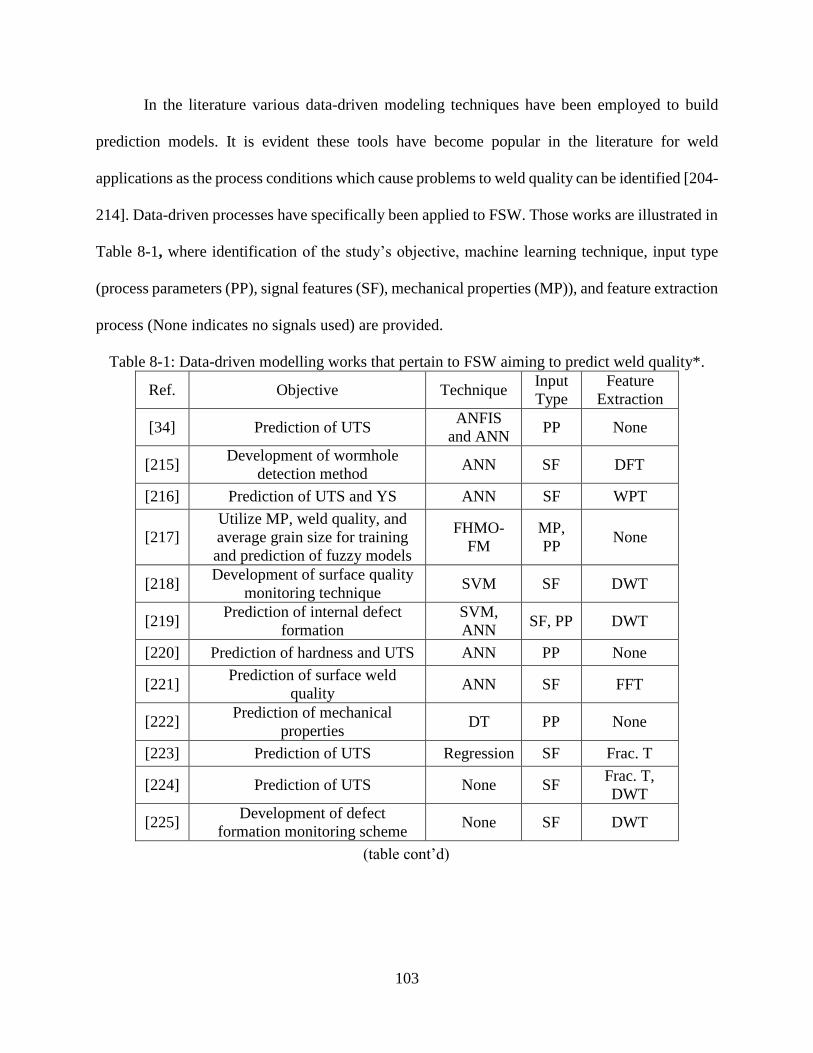
103

In the literature various data-driven modeling techniques have been employed to build

prediction models. It is evident these tools have become popular in the literature for weld

applications as the process conditions which cause problems to weld quality can be identified [204-

214]. Data-driven processes have specifically been applied to FSW. Those works are illustrated in

Table 8-1, where identification of the study’s objective, machine learning technique, input type

(process parameters (PP), signal features (SF), mechanical properties (MP)), and feature extraction

process (None indicates no signals used) are provided.

Table 8-1: Data-driven modelling works that pertain to FSW aiming to predict weld quality*.

Ref. Objective Technique Input

Type

Feature

Extraction

[34] Prediction of UTS ANFIS

and ANN PP None

[215] Development of wormhole

detection method ANN SF DFT

[216] Prediction of UTS and YS ANN SF WPT

[217]

Utilize MP, weld quality, and

average grain size for training

and prediction of fuzzy models

FHMO-

FM

MP,

PP None

[218] Development of surface quality

monitoring technique SVM SF DWT

[219] Prediction of internal defect

formation

SVM,

ANN SF, PP DWT

[220] Prediction of hardness and UTS ANN PP None

[221] Prediction of surface weld

quality ANN SF FFT

[222] Prediction of mechanical

properties DT PP None

[223] Prediction of UTS Regression SF Frac. T

[224] Prediction of UTS None SF Frac. T,

DWT

[225] Development of defect

formation monitoring scheme None SF DWT

(table cont’d)

104

Ref. Objective Technique Input

Type

Feature

Extraction

[226] Development of defect

formation monitoring scheme None SF Fract. T

[227]

Development of acoustic

emission defect formation

monitoring scheme

None SF FFT, STFT,

DWT

*(ANFIS-Adaptive Neuro-fuzzy Inference System, ANN-Artificial Neural Network, DFT-Discrete Fourier

Transform, Frac. T-Fractal Theory, DT-Decision Tree, DWT-Discrete Wavelet Transform, FFT-Fast

Fourier Transform, STFT-Short-Time Fourier Transform, FHMO-FM-Fast Hierarchical Multi-Objective

Fuzzy Modeling, SVM-Support Vector Machine, UTS-Ultimate Tensile Strength, WPT-Wavelet Packet

Transformation, YS-Yield Strength)

The works in Table 8-1 illustrate data-driven modeling techniques can accurately predict

weld quality. In this work the data-driven techniques of K-Nearest Neighbor (KNN) and Fuzzy

KNN (FKNN) are employed with both K-fold and leave-one-out cross validation (LOOCV).

Furthermore, the artificial bee colony (ABC) was used to provide the feature selection ability to

enhance the classification techniques. The only study that has employed ABC in FSW application

is [228], in which ABC was utilized to optimize fuzzy prediction models, not feature selection.

Moreover, in our study ABC is utilized not only for feature selection, but also for optimization of

the K-value in KNN or FKNN which to the author’s knowledge is the first time this is

accomplished for FSW applications.

Features of various FSW signals have been utilized for weld quality prediction as seen in

Table 8-1. Some studies used only process parameters whereas others used only signal features.

The study of Das et al. [219] is the only one that makes use of both process parameters and signal

features. Our study differs from [219] in several aspects: material welded (AA-2219 vs. AA-1100),

welding control method (load-control vs. position-control), signals acquired during welding

(multiple vs. torque only), weld quality data (3-class vs. 2-class), model output (quality vs. tensile

strength), modeling method (KNN vs. SVM), and feature selection (yes vs. no). The new

contributions of this study include:

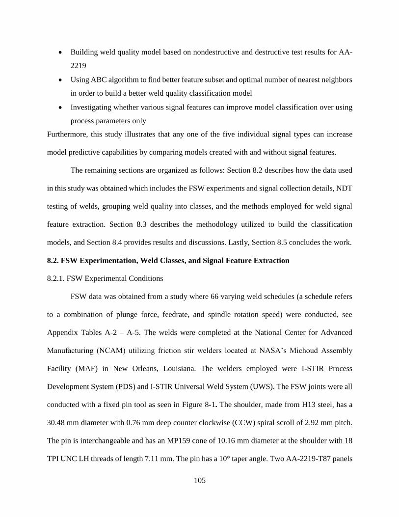
105

Building weld quality model based on nondestructive and destructive test results for AA-

2219

Using ABC algorithm to find better feature subset and optimal number of nearest neighbors

in order to build a better weld quality classification model

Investigating whether various signal features can improve model classification over using

process parameters only

Furthermore, this study illustrates that any one of the five individual signal types can increase

model predictive capabilities by comparing models created with and without signal features.

The remaining sections are organized as follows: Section 8.2 describes how the data used

in this study was obtained which includes the FSW experiments and signal collection details, NDT

testing of welds, grouping weld quality into classes, and the methods employed for weld signal

feature extraction. Section 8.3 describes the methodology utilized to build the classification

models, and Section 8.4 provides results and discussions. Lastly, Section 8.5 concludes the work.

8.2. FSW Experimentation, Weld Classes, and Signal Feature Extraction

8.2.1. FSW Experimental Conditions

FSW data was obtained from a study where 66 varying weld schedules (a schedule refers

to a combination of plunge force, feedrate, and spindle rotation speed) were conducted, see

Appendix Tables A-2 – A-5. The welds were completed at the National Center for Advanced

Manufacturing (NCAM) utilizing friction stir welders located at NASA’s Michoud Assembly

Facility (MAF) in New Orleans, Louisiana. The welders employed were I-STIR Process

Development System (PDS) and I-STIR Universal Weld System (UWS). The FSW joints were all

conducted with a fixed pin tool as seen in Figure 8-1. The shoulder, made from H13 steel, has a

30.48 mm diameter with 0.76 mm deep counter clockwise (CCW) spiral scroll of 2.92 mm pitch.

The pin is interchangeable and has an MP159 cone of 10.16 mm diameter at the shoulder with 18

TPI UNC LH threads of length 7.11 mm. The pin has a 10° taper angle. Two AA-2219-T87 panels

106

with dimensions 609.6 mm long, 152.4 mm wide, and 8.13 mm thick were friction stir welded in

a butt joint configuration with the pin tool set with a 0° lead angle and zero offset from the weld

centerline.

Figure 8-1: A) FSW configuration employed in this work during operation illustrating the three

process parameters that compose a weld schedule; B) an image of the fixed pin tool illustrating

pin and shoulder.

8.2.2. Weld Quality Classification and Empirical Indices

After welding, welds were tested with non-destructive evaluation (NDE) and destructive

techniques in order to classify the weld quality corresponding to a particular weld schedule.

Commonly used NDE techniques include ultrasonic testing, phased array ultrasonic testing

(PAUT), X-ray radiography, liquid dye penetration tests, Eddy current testing and magnetic

particle testing. Both PAUT and X-ray radiography were used in our research project. Further

details of the NDE practices involved in this work can be found in [121, 229]. After the NDE

processes were completed, weld specimens were sectioned with a metal-cutting saw into tensile

and macrograph coupons. Tensile coupons were destructively tested with an MTS 810 Material

Test System to obtain mechanical properties. Hardness and fracture surface analysis was also

107

conducted as reported in [34]. Optical macro- and micrograph specimens were fine polished then

etched with Keller’s reagent.

Defects obtained from the welds made include trenching (TR), wormhole (WH), incomplete

penetration (IP), underfill/flash (UF/F), and internal void (IV) defects. The weld quality classes

were divided into three categories: Hot, Nominal, and Cold. This categorization is based upon the

impact that the process parameters have on the joint quality and observable defects. Hot welds

have relative characteristics of excessive heat input introduced by high spindle rotational speed,

low feedrate, and high plunge force. Hot welds exhibited UF/F defects where metal was expelled

from the weld seam. Internal voids were also found in this category located in the stir zone on the

advancing side (AS) of the weld. Alternatively, cold welds are attributed to low heat input caused

by low spindle rotational speed, high feedrate, and low plunge force. A cold weld schedule

produces the WH, IP, and TR defect types. Lastly, nominal welds refer to welds with no detectable

defects. Figure 8-2 illustrates as-welded panel surfaces and transverse sectional macrographs of

selected specimens from each category.

Figure 8-2: Plan surfaces (left) and transverse sections (right) of a Nominal, Hot, and Cold weld

specimen.

108

Once each weld was evaluated and classified, trends in the data that could be related to

individual process parameters were observed. In order to create a link between these parameters,

a pin speed ratio (PSR) and a parameter coined empirical force index (EFI) that encompasses all

three process parameters with pin tool geometric conditions was devised [34]. These two relations

can be observed in Equations 1 and 2.

𝑃𝑆𝑅 = 2𝜋𝑟 ∙𝜔

𝑉 (8.1)

𝐸𝐹𝐼 =𝐹𝑧

𝐶1(𝑃𝑆𝑅)−𝐶2 (8.2)

where V denotes feedrate, ω is spindle rotational speed, r is the pin radius, 𝐹𝑧 is plunge force, and

𝐶1 and 𝐶2 are constants obtained from the curve of nominal experimental data points from the

process parameter plot in Figure 8-3. The classification of welds in this study can be roughly

indicated by the EFI. The EFI relation determines if the process parameters are near nominal

welding conditions. If the value is near 1, nominal welding conditions should occur. If the EFI

value deviates from unity, then the weld quality deteriorates. The EFI is meant to be utilized to

estimate weld quality with few data points to help guide the prediction of nominal welding

conditions. In [34], the EFI was employed to obtain defect free joints. This relation is valuable for

modeling as it relates the three process parameters for FSW. The numerical ranges for each quality

classification can be observed in Table 8-2. The constants 𝐶1 and 𝐶2 in this study were found to

be 245.43 and 0.551 respectively.

Table 8-2: Weld quality values for EFI with associated averages. EFI Range Average

Cold 0.68 – 0.96 0.83

Nominal 0.87 – 1.11 1.00

Hot 1.08 – 1.77 1.26

109

Figure 8-3: Process parameter window illustrating weld quality classes and the boundaries

between hot and nominal as well as cold and nominal weld conditions.

It is observed there is overlap in EFI values for regions approaching 1.00. In this region

overlapping EFI values are due to the boundary that dictates a hot/nominal and cold/nominal weld

condition. From the ranges above, the overlap of maximum and minimum EFI values for cold-

nominal conditions has a range of 0.09 and for nominal-hot 0.03. The determination of quality in

these regions are dictated by mechanical properties and observed defects. At these regions there is

a propensity for process parameters to create either nominal or inferior properties. In order to zero-

in on these boundaries, many more experiments must be conducted and were not able to be further

investigated in this study due to budget constraints. The EFI ranges with respect to mechanical

properties can be visualized in Figure 8-4.

110

Figure 8-4: Weld quality classes based upon EFI, UTS, and Toughness.

8.2.3. FSW Signal Features

During the welding process FSW signals were recorded at a sampling rate of 60 Hz by the

welding machines that include X-force, Y-force, plunge force, RPM, and feedrate. Typically in

manufacturing settings signal data is only viewed with a low sampling rate, i.e. 10 Hz. However,

it was conjectured that this signal data sampled at higher rates might lead to indication of defects

or instability in a weld due to the information that can be obtained from the variation in signal data.

As an example, Figure 8-5 illustrates a weld where a defect has occurred. In this weld, the initial

111

plunge stage creates a defect free welding environment as adequate pre-heating of material near

the pin tool occurs in the plunge and dwell stage. As the pin tool traverses the seam, the heat

generated from those stages dissipates leading to a defective weld roughly 150 mm into the weld.

The force signals have a sudden change in magnitude at the point where a defect free region turns

into a defect region, as highlighted by the circle in Figure 8-5.

Figure 8-5: FSW signal data illustrating weld signal data of X-, Y-, and plunge forces indicating

the change in steady-state conditions when a TR defect forms.

The signals acquired for each weld experiment generated large data sets which poses problems

for classification algorithms. Moreover, signal data obtained during FSW is highly uniform due to

the load-control process employed in this study; consequently, a large portion of the signal data

collected is somewhat redundant. Extraction of useful features requires a signal processing

technique that will map the existence of frequency components in the signal and produce a

representation of how these components change during welding. The discrete wavelet

112

decomposition (DWD) method provides a signal processing technique that meets all the criteria

for extracting useful features from FSW signals. These features can identify frequencies and their

magnitudes at specific points in time and can be represented in multiple resolutions. For this

reason, the DWD method was employed to analyze the weld signals acquired during FSW

experiments.

Before the application of DWD, the original FSW signals were segmented into discrete

segments. Segmentation is conducted in a way to ensure no overlapping of windows occurs and

the data size in each window will change for varying feedrates. Wavelet methods were thereafter

applied separately to each window. In this work, the first order Daubechies (Haar) wavelet was

chosen as the mother wavelet due to its computational efficiency. The basis of DWD is the filtering

schemes which provide the capability to decompose the original signal into different details as

seen in Eqs. (3) and (4).

𝑦𝐻𝑖𝑔ℎ𝑃𝑎𝑠𝑠𝐹𝑖𝑙𝑡𝑒𝑟(𝑘) =∑𝑥(𝑛) ∙ 𝑔(2𝑘 − 𝑛)

𝑛

(8.3)

𝑦𝐿𝑜𝑤𝑃𝑎𝑠𝑠𝐹𝑖𝑙𝑡𝑒𝑟(𝑘) =∑𝑥(𝑛) ∙ ℎ(2𝑘 − 𝑛)

𝑛

(8.4)

Upon the completion of the wavelet calculation for one window, the output was saved and the

process was repeated for adjacent windows until all windows undergo wavelet transformation.

This process was repeated for up to five levels of decomposition to construct five sets of details

for each signal type. The energy of each decomposed set of details is computed as the sum of the

squares of its values. Hence, for each segment of weld five energy values are extracted from each

signal. Exact details of this feature extraction process can be founded in [230], and part of the

resultant features employed in this study are given in Appendix Tables A-2 – A-5.

113

8.3. Classification Methodology

Two classification algorithms, specifically KNN and FKNN, were employed to build

classification models utilizing only process related parameters first, and then with additional signal

features later for potential classification accuracy improvement. In this work, the number of folds

for cross validation are varied from 2-fold, 10-fold, to LOOCV to determine best classification

result. The reason for employing these three was decided to double check whether different folds

would lead to different results. These techniques are popular in the literature, and are utilized to

evaluate the performance of classification algorithms; however, attention to the approaches for

making statistical inferences must be considered when using said techniques [231] such as the

number of folds, number of instances in a fold, the averaging for accuracy estimation, and the

repetition of k-fold cross validation. KNN and FKNN are known lazy learning methods with only

one model parameter, i.e. K. These techniques were selected for this study due to their ease of use,

and no need for training the model in serving as the classifier in the wrapper approach of

metaheuric-based feature selection.

Metaheuristics, which are high level strategies for exploring search spaces is a proven

technique to determine the optimal feature subsets and can be exercised to optimize a classification

modelling scheme. Feature selection is a promising technique for building a better classification

model with fewer more discriminant features, and such an approach has been successfully applied

to weld applications to produce good results [206, 232, 233]. In order to improve classification

accuracy a proven metaheuristic algorithm ABC [234] is chosen for this study to be employed for

not only feature selection but also optimizing model parameter K of KNN and FKNN. It is noted

that ABC has been employed for feature selection in past works [235-238], but none on weld

quality prediction. Two of these three papers employed KNN as the classifier, but the K value in

114

these works was not optimized but assumed to be one. In [235], ABC was utilized to select features

to classify UCI repository data sets such as image segmentation, automotive, and health issues. In

that study, results indicate that a reduced number of features can achieve improved classification

accuracy compared to using every feature. ABC outperformed other algorithms in 8 out of 10

tested data sets. Another study employed ABC for feature selection, and utilized SVM to classify

images in medical applications [236]. In that study, it was determined said method is more

successful compared to other pattern recognition algorithms. Reference [239] utilized ABC to

perform feature selection on bioinformatics. In that study, KNN was employed for fitness

evaluation and found high classification accuracy for large and small data sets. Another study

employed ABC coupled with neural network as the classifier to select optimal feature subsets

[237]. The feature selection technique was tested on six datasets from UCI machine learning

repository. Comparing ABC with other optimization techniques coupled with neural network, it

was found that ABC obtained best performance.

It is evident ABC is a suitable technique for feature selection and is quite useful when

coupled with a classification method. Furthermore, ABC is widely accepted due to its

straightforward implementation and it has few control parameters. The ABC algorithm imitates

honey bee’s behavior in selecting food sources. To accomplish this, bees are divided into three

groups that include the employed, onlooker, and scout bees. The food source in ABC represents a

solution in optimization problems, which is a feature subset in the context of this study. An outline

of the algorithm and functions of the bee groups are presented below:

Start:

Initialize Solutions

Repeat

115

1) Employed Bees Process

Update and Evaluate Feasible Solutions

2) Onlooker Bees Process

Select Feasible Solutions

Update and Evaluate Feasible Solutions

3) Scout Bee Process

Avoid Sub-optimal Solutions (Replace them with Randomly Generated Solutions)

Continue until maximum number of iterations/stopping criterion met

End

The number of employed bees is equal to the number of food sources, i.e. solutions to an

optimization problem. The employed bees determine the probability value of sources and share

the information with the onlooker bees. The probability of a food source (or feature subset solution)

i is computed as:

𝑝𝑖 = 0.9 ∗

𝑓𝑖𝑡𝑛𝑒𝑠𝑠𝑖max∀𝑖(fitness𝑖)

+ 0.1 (8.5)

𝑓𝑖𝑡𝑛𝑒𝑠𝑠𝑖 =

1

𝑒𝑟𝑟𝑖 + 1 (8.6)

Where erri denotes the error rate for a feature subset solution i, computed as the number of

misclassified data points over number of tested data points.

Thereafter, the onlooker bees use said information to determine whether a particular food

source should be pursued. Both employed and onlooker bees use the following equation to generate

a new solution vi from xi [240].

𝑣𝑖𝑗 = 𝑥𝑖𝑗 + ∅𝑖𝑗(𝑥𝑖𝑗 − 𝑥𝑘𝑗) (8.7)

116

where k is a randomly selected solution different from i (or food source visited by a bee), j is a

randomly selected dimension, and ij is a random number [-1, 1]. The scout bees are responsible

for searching for new food sources, and the new solution is often randomly generated.

The ABC algorithm was originally developed for continuous optimization. To use it for

feature selection, real values between zero and one are rounded into binary with 1(0) indicating a

feature selected (not selected). The K values range from 1 to half of the total number of data records

and a rounding operation has to be applied to convert a real-coded K into an integer K as well.

8.4. Results and Discussion

8.4.1. Stand-alone Classifier Model verses Metaheuristic with Classifier Wrapper

At the on-set of the work KNN and FKNN were tested to determine which classification

algorithm would produce the best result. In other words, all process parameters related features are

employed without feature selection. The K value is assumed to be 1 for both KNN and FKNN. It

was observed that KNN outperformed FKNN in all cases regardless of the cross validation scheme.

The general trend of increasing classification accuracy is expected as the number of folds

increases, as shown in Table 8-3. The classification error is the ratio of number of errors and

number of data points tested over all k-fold tests. The predictability of the model is of interest here;

hence, the model training error was not computed.

Table 8-3: Classification error rates for weld quality utilizing KNN and FKNN with all features.

K-Fold=2 K-Fold=10 LOOCV

Classification

Error [%]

Classification

Error [%]

Classification

Error [%]

KNN 35.53 28.57 25.40

FKNN 40.79 32.86 33.33

In order to improve classification accuracy, ABC was employed for selecting near-optimal

feature subset and obtaining a near-optimal K value. Table 8-4 illustrates the results by varying

the three CV schemes and population size. Simulations were extended until convergence was

117

achieved as seen in Figure 8-6. The maximal number of evaluations was set at 10,000, which is a

bit too large because the convergence seems to occur early. To capture the stochastic nature of

ABC, ten runs were made. Comparing Table 8-4 with Table 8-3, it is observed that model

classification error rates are lower when KNN and FKNN are used together with ABC-based

feature selection, regardless the CV scheme. When the ABC metaheuristic is applied to determine

the features to be utilized and the optimal K value in the classification algorithm, classification

error reduces.

Table 8-4: Classification error rates of weld Quality for KNN and FKNN coupled with

Metaheuristic ABC.

Population Size=5


Avg.

Classification

Error [%]

St.

Dev.

Avg.

Classification

Error [%]

St.

Dev.

Avg.

Classification

Error [%]

St.

Dev.

KNN + ABC 19.16 0.01 11.73 0.03 8.40 0.04

FKNN + ABC 24.21 0.01 13.69 0.02 11.54 0.03

Population Size=10


Avg.

Classification

Error [%]

St.

Dev.

Avg.

Classification

Error [%]

St.

Dev.

Avg.

Classification

Error [%]

St.

Dev.

KNN + ABC 18.74 0.01 10.54 0.02 6.84 0.01

FKNN + ABC 23.81 0.01 13.19 0.01 9.97 0.01

Population Size=15


Avg.

Classification

Error [%]

St.

Dev.

Avg.

Classification

Error [%]

St.

Dev.

Avg.

Classification

Error [%]

St.

Dev.

KNN + ABC 18.79 0.01 11.01 0.03 7.19 0.02

FKNN + ABC 23.92 0.04 14.04 0.02 10.97 0.03

The results in Table 8-4 illustrate the average classification error and standard deviation

for 10 runs of the ABC algorithm. In the majority of cases with KNN, the optimal k-value obtained

was 1. In few cases, namely when the k-fold=2 technique was employed, the optimal K-value

varied from 6 to 9. Furthermore, the best feature subset obtained from each case also varied when

118

k-fold=2, but were all similar when k-fold=10 and when LOOCV was employed. This trend

remained the same as the population size increased. On the other hand, for FKNN the optimal K-

value varied from 6 to 7 when k-fold=2. In every other CV technique, the optimal K-value obtained

varied from 1 to 2. The best feature subsets for each case regardless of the CV technique and

population size remained the same.

Figure 8-6: Convergence profile of KNN + ABC where population size=10 with 10-Fold CV.

The results indicate that the best model achieved the average classification error of 6.84%

based on LOOCV when KNN is coupled with ABC using a population size of 10. The best feature

subset included rotational speed, feedrate, and EFI with optimal K value of 1. KNN again

outperforms FKNN and accuracy again increases with number of folds. The low standard deviation

values indicate the consistency of the ABC algorithm in producing similar results. Comparing the

results of three population sizes, the population size of 10 appears to be the best.

The weld schedules (or process parameters) which promote the decrease in weld

classification accuracy are identified in Table 8-5. These have been identified as weld schedules

which are on the boundaries between hot/nominal and cold/nominal welds as discussed in the

above section. At this region the quality of a weld schedule is hard to predict as the process

119

parameter combination may or may not lead to a nominal weld, as seen in the process parameter

window in Figure 8-3. In the nominal weld region the combination of weld parameters provides

sufficient heat and mechanical deformation to join the faying surfaces of the two workpieces. If

any one of these parameters are varied the material flow characteristics will change and cause

adverse properties. For certain weld parameter combinations, there is a region where the

combination begins to degrade the joint quality. As an example, if rotational speed and feedrate

are taken to be constant and the plunge force is varied, a clear difference in weld quality will be

obtained going from low to high. Alternatively, taking the plunge force to be constant, and varying

the combination of rotational speed and feedrate the weld quality will also be altered. These

combinations of weld parameters are more sensitive at the hot/nominal and cold/nominal

boundaries. This is why in industry and production settings considerable time and effort are

employed to choose the best weld schedule for an application, and one that is conservative in that

the process parameter combination, if altered due to an anomaly, will retain satisfactory joint

quality.

To illuminate the inaccuracy of the boundary regions (points located at the boundary are

prone to classification error) the aforementioned modeling and testing schemes were repeated

without the boundary data sets that breach into the nominal weld region. Thus, any data points

classified with an EFI outside the range of 0.68-0.87 for cold welds and 1.11-1.77 for hot welds

were temporarily removed (8 cold welds and 3 hot welds) for demonstration purposes (They are

put back in the subsequent tests). The results of this test can be observed in Table 8-6 and 7.

Comparing Table 8-6 with Table 8-3, and Table 8-7 with Table 8-4, it can be found that

classification accuracy increases for all cases when boundary data points are removed. KNN again

outperforms FKNN and accuracy again increases with number of folds. The low standard deviation

120

values again indicate the consistency of the ABC algorithm in producing similar results.

Comparing the results of three population sizes, population size of 15 appears to be the best but is

only slightly better than 10.

The best feature subset produced which obtained the best classification accuracy was EFI

alone with a K value of 2. This result is intuitive as EFI incorporates all three process parameters

and now better defines the quality due to omitting the boundary region overlap data. This

illuminates the difficulties employing only input features of rotational speed, feedrate, plunge

force, and relations which incorporate those three parameters. Ideally, if the boundary regions are

definitive then high accuracy rates can be achieved as seen here. However, in reality this is not the

case because the boundary regions near defect and defect free welding conditions are blurry. To

circumvent the issue of the boundary region classification, weld signal features were subsequently

added to the input data pool to determine if an improved classification model could be constructed.

Table 8-5: Weld schedules which promote inacurrate classification due to having a combination

of process parameters which lie on the boundaries of hot/nominal and cold/nominal weld quality

(3 – Hot Weld, 8 – Cold Weld).

RPM Feedrate

[mm/min]

Plunge

Force

[kN]

Quality

Class

300.00 152.40 27.80 3

300.00 152.40 27.58 3

400.00 228.60 28.91 3

450.00 76.20 14.46 2

200.00 152.40 27.58 2

300.00 101.60 17.79 2

200.00 135.38 26.69 2

200.00 203.20 33.36 2

250.00 170.18 26.69 2

450.00 152.40 18.24 2

250.00 76.20 17.79 2

121

Table 8-6: Classification error rates for weld quality utilizing KNN and FKNN with all features

without boundary data sets.


Classification

Error [%]

Classification

Error [%]

Classification

Error [%]

KNN 25.93 21.30 22.92

FKNN 34.03 25.00 24.20

Table 8-7: Classification error rates of weld Quality for KNN and FKNN coupled with

Metaheuristic ABC without boundary data sets.

Population Size=5


Avg.

Classification

Error [%]

St.

Dev.

Avg.

Classification

Error [%]

St.

Dev.

Avg.

Classification

Error [%]

St.

Dev.

KNN +ABC 3.70 0.00 2.50 0.00 2.70 0.01

FKNN

+ABC 16.67 0.00 15.50 0.02 16.02 0.01

Population Size=10


Avg.

Classification

Error [%]

St.

Dev.

Avg.

Classification

Error [%]

St.

Dev.

Avg.

Classification

Error [%]

St.

Dev.

KNN +ABC 3.70 0.00 2.5 0.00 2.26 0.00

FKNN

+ABC 16.67 0.00 14.70 0.03 15.26 0.01

Population Size=15


Avg.

Classification

Error [%]

St.

Dev.

Avg.

Classification

Error [%]

St.

Dev.

Avg.

Classification

Error [%]

St.

Dev.

KNN +ABC 3.70 0.00 2.39 0.00 2.18 0.00

FKNN

+ABC 16.67 0.00 14.01 0.02 15.44 0.01

8.4.2. Weld Signal Features Added to Classification Models

Weld signals are important to understand the quality of a weld. During the weld process, it

is standard practice for the operator to monitor weld signals to ensure forces acting on the pin tool

does not exceeding a predetermined value based upon weld tooling. Furthermore, viewing the

fluctuations in signal values can indicate quality of the weld as observed by previous research

122

summarized in Table 8-1. The operator has the discretion to abort a weld if a target value or large

fluctuation in a particular weld signal is observed. This study attempts to show that automatic

interpretation of weld signals can greatly assist the operator in predicting the quality of a weld.

Our study aims to use signal features to strengthen the correlation between the three process

parameters and weld quality. As discussed in Section 2, DWD was employed to obtain these

features. In total, five signal types including X-force, Y-force, plunge force, rotational speed, and

feedrate signals were fed into the DWD algorithm window by window to extract features. For each

signal type, 5 decomposition levels were obtained. The window size for DWD was computed as a

function of weld travel distance rather than time. Features from three of these windows were

chosen based upon three locations at the start, middle, and end of the weld to ensure features at all

locations of the weld are caught.

In order to determine the weld signal features which promote the best classification result,

the set of five features from each signal were added to the set of process parameters and tested

with KNN and FKNN classifiers. To avoid redundancy, the tests conducted here utilized only

LOOCV. The population size of the ABC algorithm was increased to 20 as a larger data set was

fed into the model classification scheme.

A summary of results from 10 runs are given in Table 8-8 with best feature subset and

optimal K value. In all cases with KNN the optimal K-value obtained was 1; however, the best

feature subset varied from run to run. The best features reported in Table 8-8 are the most common

obtained from the 10 runs. For KNN, the best feature subset was obtained 5 times for plunge force

wavelet features (WFs), 6 times for x-force WFs, 4 times for y-force WFs, 4 times for RPM WFs,

and 4 times for feedrate WFs. On the other hand, for FKNN the optimal k value deviated from 1

for cases that employed RPM and x-force WFs. However, the most common k-value obtained in

123

those cases was 1. The best features listed in Table 8-8 for FKNN were obtained 5 times for plunge

force WFs, 4 times for x-force WFs, 3 times for y-force WFs, 4 times for RPM WFs, and 6 times

for feedrate WFs.

It was found that adding weld signal features significantly improved the classification

accuracy. In 7 of the 10 cases, 100% accuracy was obtained. In the three cases which did not obtain

100% accuracy, the FKNN technique was utilized as the classifier. Overall, incorporating weld

signal features to the model improved the accuracy and mitigates the issues that the boundary

region creates for the model. Comparing the result of each set of wavelet signal features, it appears

that each provides the best result when KNN is applied. However, if FKNN is taken as the

classification technique then plunge force, X-Force, and feedrate signal features should not be

utilized. For this reason when developing a classification algorithm for FSW, utilization of weld

signal features should be conducted to produce the best model for predicting weld quality more

accurately.

Among the seven cases that yield perfect classification accuracy, the best case can be

chosen to be the one with lowest number of features. Consequently, the best feature subset

comprised of plunge force, pin speed ratio, and the first wavelet feature of the x-force signal (the

third row in Table 8-8) should be used to build the 1-NN model. The next best model is the Fuzzy

1-NN model built with four features, which are PSR, EFI, and the first and second wavelet features

of the y-force signal (the sixth row in Table 8-8).

124

Table 8-8: Classification error rates of weld Quality for KNN and FKNN coupled with Metaheuristic ABC employing additional

features obtained from weld signals.

Features Added

Best Feature Subset (found by the ABC algorithm) Classification

Error

K

Number RPM

FR

[mm/min]

PF

[kN] PSR

EFI

[kN]

WF

1

WF

2

WF

3

WF

4

WF

5

Mean

[%]

St.

Dev.

Plunge

Force

Wavelet

Features

K-NN 1 √ √ √ √ √ √ 0.0 0.0

Fuzzy

K-NN 1 √ √ √ √ √ √ √ √ 22.50 0.0

X-Force

Wavelet

Features

K-NN 1 √ √ √ 0.0 0.0

Fuzzy

K-NN √ √ √ √ √ √ 0.60 0.0

Y-Force

Wavelet

Features

K-NN 1 √ √ √ √ √ 0.0 0.0

Fuzzy

K-NN 1 √ √ √ √ 0.0 0.0

RPM

Wavelet

Features

K-NN 1 √ √ √ √ √ 0.0 0.0

Fuzzy

K-NN 1 √ √ √ √ √ 0.0 0.0

Feedrate

Wavelet

Features

K-NN 1 √ √ √ √ √ √ √ 0.0 0.0

Fuzzy

K-NN 1 √ √ √ √ √ √ 12.33 0.01

125

8.5. Conclusions

This work has presented the results obtained in a study to build a reliable and highly

accurate weld quality prediction model. From an extensive experimental FSW study, KNN and

FKNN based classification models for weld quality prediction were built employing weld process

parameters, a pin speed ratio, an empirical relation, and wavelet features extracted from weld

signal data. Employing only the welding process parameters as inputs, moderate classification

accuracy was obtained due to the fuzzy boundaries of Hot/Nominal and Cold/Nominal welds. The

test results indicate that employing the population based metaheuristic artificial bee colony,

classification accuracy improves as opposed to using all features to build classification models.

100% classification accuracy was obtained utilizing ABC with KNN or ABC with FKNN while

incorporating weld signal features. In order to build the best model with highest classification

accuracy, weld signal features should be employed together with process parameters.

A high number of classification models and metaheuristic algorithms have been developed.

If used properly, it is expected that any combination will achieve similar results as reported in this

study, though they might differ in the best result. Since 100% accuracy has been achieved in the

study, no attempt in using other combinations of classification model and metaheuristic is

necessary. However, the combination used in this study might not be the best for another

application.

126

CHAPTER 9 : DEFECT SUPPRESSION MODEL FOR FIXED PIN FSW

Genius is one percent inspiration and ninety-nine percent perspiration

-Thomas A. Edison

9.1. Introduction

If a rotating pin seized in a metal surface is translated, metal will flow up around the pin

and leave a furrow in the wake of the pin. In order to suppress the furrow and create a weld a

shoulder is added to the pin and held with sufficient pressure against the surface to prevent upward

flow of metal around the pin. In the basic Friction Stir Welding (FSW) process the tool shoulder

constitutes a rudimentary defect suppression device.

In FSW practice, in spite of the furrow-suppressing shoulder, defects of a more subtle

nature still occur and reduce the strength of the resultant welds. Such defects observed in a study

of 85 welds in 8.13 mm thick 2219-T87 aluminum alloy are illustrated in Figure 9-1 and correlated

with welding parameters spindle rotational speed (ω), feedrate (V), and plunge force (Fz) as

observed in Table 9-1 and Table 9-2. Trends were found in this study that related these three

parameters to the presence of defects and presented the opportunity to suppress more subtle defect

formation by varying the shoulder pressure, through the plunge force, in accordance with the

spindle rotational speed and feedrate parameters.

Table 9-1: FSW weld schedules conducted with I-Stir UWS #2 with defects (DF - defect free,

TR - Trenching defect, WH - wormhole, IP - Incomplete Penetration, UF/F - Underfill/Flash

defect, Internal voids - V).

Number

Spindle

Rotational

Speed

[RPM]

Feedrate

[mm/min]

Plunge

Force

[kN]

UTS

[MPa]

Toughness

[MJ/m³]

Estimated

Weld

Temperature

[°C]

Defects

1 200 152.4 33.36 323.31 42.18 448 DF

2 300 152.4 24.47 310.24 32.9 475 DF

3 350 76.2 15.57 331.68 44.89 493 DF

4 350 152.4 22.24 362.08 41.91 484 DF

5 350 152.4 20.02 353.98 40.07 484 DF

(table cont’d)

127

Number

Spindle

Rotational

Speed

[RPM]

Feedrate

[mm/min]

Plunge

Force

[kN]

UTS

[MPa]

Toughness

[MJ/m³]

Estimated

Weld

Temperature

[°C]

Defects

6 300 152.4 22.24 339.66 37.8 475 DF

7 350 266.7 30.25 356.36 41.78 471 DF

8 350 236.98 26.69 359.96 48.57 474 DF

9 350 118.62 19.57 347.61 44.52 488 DF

10 350 88.9 16.46 333.45 36.08 491 DF

11 300 228.6 30.25 326.33 39.64 466 DF

12 300 203.2 26.69 328.14 36.55 469 DF

13 350 152.4 17.79 172.95 4.67 484 TR/IP

14 350 152.4 15.57 166.63 4.07 484 TR/IP

15 200 152.4 26.69 283.38 15.01 448 IP

16 300 152.4 21.13 288.12 11.59 475 WH

17 300 203.2 21.13 178.06 2.38 469 TR/WH/IP

18 300 203.2 24.47 279.81 11.84 469 WH/IP

19 300 152.4 20.02 279.06 9.13 475 WH

20 300 203.2 22.24 315 17.54 469 WH

21 300 203.2 20.02 237.74 4.03 469 WH/IP

22 450 152.4 33.36 260.17 9.09 496 Void/UF/F

23 450 152.4 28.91 290.59 10.83 496 Void/UF/F

24 450 152.4 35.59 211.72 4.12 496 Void/UF/F

Table 9-2: FSW Weld Schedules conducted on I-Stir PDS Welder with Associated

Characteristics (DF - defect free, TR - Trenching defect, WH - wormhole, IP - Incomplete

Penetration, UF/F - Underfill/Flash defect, Internal voids - V).

Number

Spindle

Rotational

Speed

[RPM]

Feedrate

[mm/min]

Plunge

Force

[kN]

UTS

[MPa]

Toughness

[MJ/m³]

Estimated

Weld

Temperature

[°C]

Defects

25 350 76.2 14.46 320.25 30.79 493 DF

26 350 76.2 16.68 324.41 33.72 493 DF

27 200 152.4 31.14 313.99 45.51 448 DF

28 300 203.2 26.69 318.59 27.52 469 DF

29 350 88.9 15.57 326.84 37.48 491 DF

30 300 152.4 21.69 335.87 43.85 475 DF

31 350 76.2 14.01 355.87 33.52 493 DF

32 300 130.56 24.47 333.74 30.89 478 DF

33 300 101.6 22.24 335.62 35.87 482 DF

34 300 76.2 17.79 320.65 31.23 485 DF

35 400 101.6 17.79 337.37 37.8 496 DF

36 400 76.2 15.57 327.46 35.02 498 DF

37 350 88.9 17.79 343.43 47.42 491 DF

(table cont’d)

128

Number

Spindle

Rotational

Speed

[RPM]

Feedrate

[mm/min]

Plunge

Force

[kN]

UTS

[MPa]

Toughness

[MJ/m³]

Estimated

Weld

Temperature

[°C]

Defects

38 350 152.4 22.24 352.29 33.76 484 DF

39 350 152.4 20.02 349.41 33.53 484 DF

40 350 152.4 24.47 340.99 39.79 484 DF

41 400 76.2 14.68 317.9 24.95 498 DF

42 400 76.2 13.34 330.69 31.34 498 DF

43 250 76.2 20.91 311.93 45.95 475 DF

44 300 203.2 31.14 343.12 35.68 469 DF

45 300 203.2 33.36 347.34 34.1 469 DF

46 300 228.6 33.36 346.34 34.06 466 DF

47 300 228.6 31.14 354.05 45.24 466 DF

48 400 228.6 24.47 347.44 29.34 483 DF

49 400 228.6 26.69 353.71 33.44 483 DF

50 250 228.6 36.48 336.7 48.34 453 DF

51 250 228.6 40.03 346.7 49.44 453 DF

52 400 203.2 23.58 354.37 42.68 485 DF

53 400 203.2 26.69 352.83 37.18 485 DF

54 350 152.4 17.79 153.5 2.33 484 TR/IP

55 200 152.4 27.58 267.75 15.08 448 IP

56 300 101.6 16.01 167.38 6.56 482 TR/IP

57 350 76.2 12.46 157.56 5.76 493 TR/IP

58 300 76.2 14.23 176.95 7.2 485 TR/IP

59 300 101.6 17.79 192.24 6.74 482 TR

60 200 135.38 26.69 267.32 15.94 451 IP

61 200 203.2 33.36 268.33 15.34 439 IP

62 250 170.18 26.69 293.75 17.62 461 IP

63 450 152.4 18.24 289.94 11.87 496 IP and

WH

64 250 228.6 33.36 287.79 14.97 453 IP

65 300 228.6 28.91 298.28 15 466 IP

66 400 203.2 20.91 314.92 19.49 485 IP

67 250 203.2 28.91 285.38 16.3 456 IP

68 250 76.2 17.79 209.19 3.69 475 IP and

TR

69 300 228.6 35.59 335.06 30.14 466 UF/F

70 400 228.6 28.91 341.18 23.04 483 UF/F

71 350 76.2 17.79 314.44 31.65 493 UF/F

72 350 152.4 26.69 314.44 28.54 484 UF/F

73 350 88.9 20.02 315.53 22 491 UF/F

74 200 152.4 36.48 326.49 47.1 448 UF/F

75 400 76.2 16.9 336.01 24.07 498 UF/F

(table cont’d)

129

Number

Spindle

Rotational

Speed

[RPM]

Feedrate

[mm/min]

Plunge

Force

[kN]

UTS

[MPa]

Toughness

[MJ/m³]

Estimated

Weld

Temperature

[°C]

Defects

76 300 76.2 22.24 322.09 30.47 485 UF/F

77 250 76.2 23.58 315.43 42.82 475 UF/F

78 225 152.4 37.81 320.4 33.95 456 UF/F

79 300 152.4 33.36 292.16 22.05 475 UF/F

80 350 152.4 28.91 317.89 22.36 484 UF/F

81 300 101.6 24.47 309.77 23.14 482 UF/F

82 350 88.9 22.24 306.69 22.46 491 UF/F

83 350 76.2 21.35 295.15 19.53 493 UF/F

84 300 152.4 27.8 324.27 26.43 475 UF/F

85 300 152.4 27.58 317.33 27.42 475 UF/F

Figure 9-1: Left: Top views of friction stir welds: Nominal weld shows well defined ripple

pattern. Hot weld shows flash on retreating side, irregular (flash-related) variations in ripple

pattern, and lack of fill on advancing side. Cold weld shows defect inside crown suppressed

ripple formation and sporadic, small extrusions on retreating side. Right: Transverse sections of

friction stir welds: (A) Nominal weld, (B) Internal void on AS, (C) Underfill, (D) Incomplete

joining of weld seam at crown, (E) Trenching on advancing side of crown and lack of

penetration at root, (F) Wormhole on advancing side and lack of penetration at root.

9.2. Procedure

Welded specimens in this work were fabricated at the NASA Michoud Assembly Facility

(MAF) in New Orleans, Louisiana. MAF houses the National Center for Advanced Manufacturing

130

(NCAM), which contains state-of-the-art FSW machines including Process Development System

(PDS) and Universal Weld System (UWS) platforms. The welds for this study were made on two

FSW machines, the I-STIR PDS and the I-Stir UWS #2.

Workpiece material employed included AA-2219-T87 panels with dimensions 609.6 mm

long, 152.4 mm wide, and 8.13 mm thick. Two panels were welded in a typical butt-joint

configuration with a fixture that utilized a steel anvil. Steel bars were placed on the advancing side

(AS) and retreating side (RS) 38.1 mm away from weld centerline and each held in place with four

clamps. Side compression screws were used on the RS. Before welding, the panels were lightly

ground to remove the oxide layer and wiped with an alcohol solution. The welds employed a 0°

lead angle with zero index-offset from the centerline. Panels were joined with a two-piece fixed

pin tool. The shoulder, made from H13 steel, has a 30.48 mm diameter with 0.76 mm deep counter

clockwise (CCW) spiral scroll of 2.92 mm pitch. The pin, which is interchangeable, is an MP159

cone of 10.16 mm diameter at shoulder with 18 TPI UNC LH threads of length 7.11 mm. The pin

has a 10° taper angle. Figure 9-2 illustrates the FSW apparatus used to make the welds.

Figure 9-2: FSW machines used to perform welds: (A) I-Stir PDS, (B) I-STIR UWS #2. FSW in

progress between clamps and steel bars holding panel against anvil (C). Tapered pin set in

scrolled shoulder (D).

131

To save material, two weld schedules were exercised on each panel. As a consequence

there were two non-steady-state locations on the panel: a Plunge Transition Zone (PTZ) at the

onset of the FS weld, and a Schedule Transition Zone (STZ) at the weld schedule transition. It was

necessary to identify and discard PTZ and STZ as not representative of the weld conditions under

investigation. PTZ and STZ can be clearly identified from weld force data, an example of which

is shown in Figure 9-3. In the example of Figure 9-3 PTZ ends about 190 seconds into the weld

process and STZ occurs between approximately 255 and 280 seconds. The four stages of the

welding process, plunge stage, dwell stage, welding stage, and retraction stage, are identified in

Figure 9-3. After the pin and shoulder are fully seated in the plunge and dwell stages a reduced

force transient is encountered at the beginning of the weld as the tool passes through a region

heated up during the dwell stage. Weld strength data are taken from coupons cut beyond this

transient and before the beginning of the STZ and from the end of the STZ to the beginning of the

retraction stage.

Figure 9-3: Above: Forces vs. time during FSW weld process example [Schedule 1: 200 RPM,

152.4 mm/min, 33.36 kN followed by Schedule 2: 450 RPM, 152.4 mm/min, 33.36 kN]. Plunge

(Z) force, drag (X) force, and lateral (Y) force measurements are shown. PTZ and STZ can be

clearly identified. Below: Process stage associated with force observations above: (A) Pin tool

descending during initial plunge stage, (B) Pin tool rotating in place during dwell stage, (C) Pin

tool translating during welding stage, (D) Pin tool rising during retraction stage.

132

Welded panels were searched for defects by Non-Destructive Evaluation (NDE) techniques

including Phased Array Ultrasonic Testing (PAUT), X-ray radiography, and liquid dye penetrant

tests. The panels were thereafter sectioned with a metal-cutting saw into tensile and macrograph

coupons. The tensile coupons were destructively tensile tested with an MTS 810 Material Test

System. For microscopy observations coupons were polished to 0.05 microns and etched with

Keller’s reagent (1 mL HF, 1.5 mL HCL, 2.5 mL HNO3, 95 mL H2O).

9.3. Results

In total, 85 weld schedules were completed varying plunge force (load-control mode),

rotational speed, and feedrate. Among the 85 weld schedules, 45 were observed to have defects

and 40 were defect-free. The welds were classified Nominal, Hot, or Cold according to the ratio

of pin rotation rate to translation speed. (See the following section on weld temperature estimate.)

Nominal welds with no observable defects were found to exhibit best strength and

toughness. Nominal welds were found to have ultimate tensile strength and toughness values

between 311.93 - 362.08 MPa and 24.95 - 49.44 MJ/m³ respectively.

Hot welds incorporating internal voids (IV), and underfill/flash (UF/F) defects exhibited a

decrease in toughness. In several cases hot welds exhibited high tensile strength but low toughness

associated with excess expulsion of material from the weld seam or with IVs. The strength and

toughness of hot welds were in the range 211.72 - 341.18 MPa and 4.12 - 47.10 MJ/m³

respectively.

Cold welds exhibited trenching (TR), wormholes (WHs), and incomplete penetration (IP).

The strength and toughness values ranged 150.93 - 315.00 MPa and 1.51 - 19.49 MJ/m³

respectively.

133

Table 9-1 and Table 9-2 group welds made on the UWS and PDS platforms respectively,

exhibit weld schedules with associated defects and strength properties. Estimated weld

temperatures accompany the welds.

9.4. Analysis of Results

9.4.1. Weld Temperature Effects

It is common welding practice to establish combinations of parameters V and ω that yield

sound welds. These combinations present an area or “window” in V-ω coordinates for successful

welding parameter settings. Outside the window weld strength drops and defects begin to appear.

The left and right boundaries of empirically established windows often seem to take a shape like

that of Figure 9-4. The shape suggests isotherms as computed in equation 4 and points to a critical

role of temperature in determination of weld properties and defect structure. It implies that the V-

ω welding parameters affect weld strength through their effect on temperature.

Figure 9-4: Schematic representation of isotherms bounding area of parameter combinations

yielding sound friction stir welds.

Weld temperatures are fixed by a heat balance. Weld temperature rises to absorb the heat

generated by mechanical deformation imposed by the FSW tool until heat losses rising with weld

134

temperature absorb all the heat generated. At this point the temperature ceases to rise and a steady

weld temperature is reached.

The principal source of FSW power generation is taken to be deformation at the shear

surface. See Figure 9-5. It has been well established [182, 187] that under normal welding

conditions the principal deformation zone surrounding the FSW tool contracts to a sufficiently thin

region (an “adiabatic shear band”) that it can be treated as a surface, the “shear surface”. The shear

surface separates the fine-grained “nugget material” that sticks to and rotates with the tool from

the large-grained parent material of the weld panels. The nugget material initially takes the shape

of the shear surface, but additional deformation in the wake of the tool is evident in the

macrostructure of a transverse weld section. Beyond the shear surface a Thermo-Mechanically

Affected Zone (TMAZ) and a Heat Affected Zone (HAZ) can be distinguished. The grain

refinement characteristic of the nugget material is produced as the weld metal passes through the

shear surface. At the shear surface most of the dislocations formed during deformation annihilate

to produce elastic waves/heat, but some remain locked in tangles that polygonize in the heat to

form new grains.

The principal heat losses are taken to be conduction losses, estimated by conduction

through a “thick pipe” of weld metal surrounding the shear surface, and convection losses,

estimated by the power required to heat metal passing into the leading edge of the shear surface

from ambient to welding temperature. This model, illustrated schematically in Figure 9-6, is only

an approximation, but it appears to capture the physics of the FSW process well enough to enable

simple approximate quantitative estimates of weld temperatures and forces that correspond to

observed data and to yield physical insight into the FSW process.

135

Figure 9-5: Macrostructure at transverse section of FS weld showing trace of shear surface.

Above is shown schematically the shear surface and the plug of metal that rotates with the tool.

Outside the trace of the shear surface the Thermo-Mechanically Affected Zone (TMAZ) can be

distinguished by distorted parent metal. Further out is the Heat Affected Zone (HAZ) marked by

a distinct structure (and hardness) but without obvious metal distortions.

At welding conditions, where the weld metal is soft and workable, the weld metal

temperatures are close enough to melting temperature (𝑇𝑚𝑒𝑙𝑡) so that the flow stress may be

approximated by the relation:

𝜏~(−𝜕𝜏

𝜕𝑇) (𝑇𝑚𝑒𝑙𝑡 − 𝑇) (9.1)

The conduction losses are approximated by conduction through the walls of a thick-walled weld

metal pipe with the outside temperature and radius To and Ro respectively. (Refer to Figure 9-6)

Quantitatively this amounts to 2𝜋𝑘𝑤

𝑙𝑛(𝑅𝑜𝑅)(𝑇 − 𝑇𝑜). 𝑘 represents the thermal conductivity of the weld

metal.

136

Figure 9-6: Schematic model for heat balance used to approximate weld temperatures.

The convection losses are approximated by the requirement to heat the stream of metal

impinging on the shear surface to weld temperature, or 2𝑅𝑤𝑉𝜌𝐶(𝑇 − 𝑇𝑜), where 𝜌 is the weld

metal density and 𝐶 the specific heat.

The heat balance then becomes:

2𝜋𝑅2𝑤(−𝜕𝜏

𝜕𝑇) (𝑇𝑚𝑒𝑙𝑡 − 𝑇)𝜔~

2𝜋𝑘𝑤

𝑙𝑛 (𝑅𝑜𝑅 )

(𝑇 − 𝑇𝑜) + 2𝑅𝑤𝑉𝜌𝐶(𝑇 − 𝑇𝑜) (9.2)

The rise in temperature above ambient from equation (2) is:

(𝑇 − 𝑇𝑜)~

𝑅𝜔𝑉

𝑅𝜔𝑉 [1 +

𝑘

𝑅2𝜔(−𝜕𝜏𝜕𝑇) 𝑙𝑛 (

𝑅𝑜𝑅 )

] +𝜌𝐶

𝜋 (−𝜕𝜏𝜕𝑇)

(𝑇𝑚𝑒𝑙𝑡 − 𝑇𝑜) (9.3)

The dimensionless term 𝑘

𝑅2𝜔(−𝜕𝜏

𝜕𝑇)𝑙𝑛(

𝑅𝑜𝑅) is small compared to 1. For the above computations, it

ranges from about 0.07 to 0.15. Hence the dimensionless quantity 𝑅𝜔

𝑉 , the ratio of surface speed

137

of the rotating plug of metal attached to the tool to the feedrate, is an approximate indicator of

weld temperature. 𝑅𝜔

𝑉 is also a measure of the amount of rotation of the tool per unit travel

distance. The energy input increases with the rotations of the tool (although not in linear

proportion) as the flow stress drops as the weld heats up. For very high values of 𝑅𝜔

𝑉, the weld

temperature 𝑇 approaches the melting temperature 𝑇𝑚𝑒𝑙𝑡 and for very low values it remains at

ambient temperature, 𝑇𝑜.

It is significant that the temperature estimate of equation 3 does not depend upon the plunge

force. Because the shear stress of a metal does not depend significantly upon pressure, the torque

exerted by the FSW tool on the weld metal, 2𝜋𝑟2𝜔𝜏 in the simplified rotating cylinder model

above, should not depend upon plunge force. Schmidt et al [197] reports observations confirming

this, from which they draw the conclusion that weld metal does not slip on the tool-metal surface

where a friction coefficient would create a dependence between plunge force and torque, but rather

sticks to the tool surface, shearing taking place within the weld metal as has been assumed here.

If the weld temperature is constant, then weld isotherms have the straight-line form

represented in Figure 9-4. The quantities in brackets in equation 4 are constants.

𝑉~ [𝜋𝑅

𝜌𝐶(−

𝜕𝜏

𝜕𝑇) (𝑇𝑚𝑒𝑙𝑡 − 𝑇

𝑇 − 𝑇𝑜)]𝜔 − [

𝜋𝑘

𝑅𝜌𝐶𝑙𝑛 (𝑅𝑜𝑅 )

] (9.4)

It is possible to estimate a temperature for any parameter combination from equation 3 if

the parameters are known. The parameter values used in the weld temperature estimates presented

in Table 9-1 and Table 9-2 are given in Table 9-3.

From equations 1 and 2 the shear stress at the weld may be estimated:

138

𝜏~ [(−𝜕𝜏

𝜕𝑇) (𝑇𝑚𝑒𝑙𝑡 − 𝑇𝑜)]

{

𝑅𝜔

𝑉 [𝑘


𝑅𝑜𝑅)] +

𝜌𝐶

𝜋 (−𝜕𝜏𝜕𝑇)

𝑅𝜔𝑉 [1 +

𝑘


𝑅𝑜𝑅)] +

𝜌𝐶

𝜋 (−𝜕𝜏𝜕𝑇)}

(9.5)

If the 𝑘

𝑅2𝜔(−𝜕𝜏

𝜕𝑇)𝑙𝑛(

𝑅𝑜𝑅) term is ignored and parameter values are inserted:

𝜏~ [(−𝜕𝜏

𝜕𝑇) (𝑇𝑚𝑒𝑙𝑡 − 𝑇𝑜)]

{

𝜌𝐶

𝜋 (−𝜕𝜏𝜕𝑇)

𝑅𝜔𝑉 +

𝜌𝐶

𝜋 (−𝜕𝜏𝜕𝑇)}

~53.67{7.517

𝑅𝜔𝑉 + 7.517

} 𝑀𝑃𝑎 (9.6)

The indentation force 𝐹𝑖 is on the order of 6(𝜋𝑅𝑆2)𝜏 [241]:

𝐹𝑖~235.0{7.517

𝑅𝜔𝑉+ 7.517

} 𝑘𝑁 (9.7)

Table 9-3: Parameters used in weld temperature estimates. Parameter Description [Unit] Value

T0 Ambient Temperature [°C] 24

Tmelt Weld Metal Melting Temperature [°C] 543

RS Shoulder Radius [m] 0.01524

R0 Radius of Ambient Temperature [m] 0.1524

R Radius of Shear Surface* [m] 0.0122

(−∂τ

∂T) Weld Metal Flow Stress [

N

m2∙℃] 103,421.17

k Weld Metal Thermal Conductivity [W

m∙℃] 121.15

C Weld Metal Specific Heat Capacity [J

kg∙℃] 860.00

ρ Weld Metal Density [kg

m3] 2,840.00

*The radius of the shear surface varies from the minimal pin radius to the shoulder radius. To use

the above model a single effective shear surface radius needs to be estimated. The effective shear

surface radius lies between the minimal pin radius and the shoulder radius. Here the effective shear

surface radius is estimated at 80% of the shoulder radius.

139

Estimated results were computed from Equation 7 and compared with experimental nominal

conditions as see in Figure 9-7. It is evident that results appear to follow experimental trends;

however, the estimated forces required for nominal welds are greater than estimated indentation

pressures by a factor of x5 for the hottest and x1.3 for the coldest conditions. Since the temperature

drops off away from the shear surface, the effective temperature is lowered and the effective flow

stress is raised for deformation under the tool shoulder. Bigger gradients and bigger corrections

would be anticipated for hotter welds as is observed in the data. Depending upon what the plunge

force is required to do to suppress defects, somewhat higher plunge forces than the computed

indentation force might well be required. Since the total volume under the shoulder is colder than

the weld temperature, the actual indentation force would be higher. Hence a correction factor 𝐹𝑧

𝐹𝑖 is

needed to account for temperature drop-off away from the shear surface in an estimation of the

upper bound for the plunge force.

𝐹𝑧 ≤𝐹𝑧𝐹𝑖6(𝜋𝑅𝑆

2)𝜏 (9.8)

A plot of estimated indentation force with 𝑅𝜔

𝑉 from equation 8 is shown in Figure 9-7. In the same

plot, experimental data points are laid out on similar coordinates with plunge force replacing

indentation force and with the points differentiated with respect to hot, cold, or nominal condition.

9.4.2. Pressure Effects

To form a solid state weld it is necessary to put the surfaces of a seam in close contact so

that the metallic bond can act to join the surfaces. This requires sufficient pressure to push down

asperities that keep normally rough surfaces apart. The pressure required would be on the order of

indentation pressure, 6𝜏. Thus, as the pressure under the tool shoulder, 𝐹𝑧

𝜋𝑅𝑆2, drops below 6𝜏, one

might anticipate the emergence of bonding defects located on the trace of the weld seam,

140

particularly at the crown or root, where the pressure may drop off [241]. One expects that when

the real indentation plunge force is attained one would see flash and a drop is properties due to

internal defects like wormholes and trenching. At plunge forces below the indentation pressure

less deformation within the weld metal is anticipated along with defects like lack of penetration.

“Lack of penetration”, typically caused by cold/low pressure, is such a defect with a lack of

bonding on the weld seam at the weld root.

Figure 9-7: Map of cold, hot, and nominal (no defects) weld conditions in coordinates of plunge

force and weld temperature indicator Rω/V. The nominal, defect-free weld conditions appear to

be bounded approximately by curves proportional to an estimated shoulder indentation pressure

at estimated weld temperature. Actual indentation pressure is larger because mean indentation

deformation temperature would be lower than the weld temperature.

At high pressure with respect to the flow stress, metal begins to squeeze out from under

the shoulder in the form of flash. But this in itself would not generate defects; if anything, it would

be expected to compact the nugget material and eliminate existing defects. Defects like porosity

and wormholes occur away from the seam; they are not initially open but must be opened by

141

tension. One needs to look for a source of tension to account for the defects observed in hot/high

pressure welds.

A promising candidate for a source of tension is the induction part of the cycle of forces

produced by an eccentric pin tool. It is this cycle that produces the ripples and the internal banding

observed in the wake of a FS weld [191, 242]. If the displacement flow rate, induced by a pin tool

of eccentricity 휀 and length w were to emerge at the weld metal surface, conservation of volume

would require a ripple amplitude of the order of 𝑅𝜔

𝑉

𝑤

𝑅𝑆휀, on the order of, perhaps 100 times the

eccentricity of the weld. An eccentricity of 0.001 inches would yield a ripple amplitude of 0.1

inches, far larger than observed. This suggests that the displacement of metal due to eccentricity

is mostly circumferential. The uniform appearance of the internal banding also suggests

circumferential displacements; displacements along the pin axis would presumably give rise to

gradation along the axis.

Hence the metal displaced by the eccentricity of the pin tool is taken to be pushed into the

rotating flow around the pin at appropriate rotational positions. Equilibrium for rotation of flow

by 90o or 𝜋

2 requires a pressure on the order of 𝜋𝜏, significantly less than, except very close to the

metal surface, the pressure to force the flow along an axial channel of length 𝑤 and thickness 𝛿,

on the order of 2𝑤

𝛿𝜏.

During induction, when the eccentric surface retreats from the weld metal and draws weld

metal back in, the pressure reverses and becomes tension. To cause a defect this tension must

overcome the static pressure imposed by the plunge force on the order of 𝐹𝑧

𝜋𝑅𝑆2 and a stress to rupture

the metal or generate porosity 𝜎𝑑𝑒𝑓. To avoid a defect, then:

142

𝐹𝑧

𝜋𝑅𝑆2 ≥ 𝜋𝜏 − 𝜎𝑑𝑒𝑓 (9.9)

Requiring that the plunge force be small enough to avoid indentation and large enough to suppress

defect formation by periodic internal tensile stresses places an upper and lower bound respectively

on the plunge force.

(𝜋 −𝜎𝑑𝑒𝑓

𝜏) 𝜋𝑅𝑆

2𝜏 ≤ 𝐹𝑧 ≤𝐹𝑧𝐹𝑖6𝜋𝑅𝑆

2𝜏 (9.10)

For there to be a defect-free nominal zone

(𝜋 −𝜎𝑑𝑒𝑓

𝜏) <

𝐹𝑧𝐹𝑖6 (9.11)

which is the case, although the difference appears to be bigger than for the data observed.

9.5. Conclusion

A study of 85 FS welds in 8.13 mm thick AA-2219-T87 aluminum alloy suggests that

defects in FS welds may be suppressed by adjusting the plunge force to maintain a fixed relation

between mean pressure under the tool shoulder to metal flow stress at welding temperature. A

simplified analysis relates flow stress to weld temperature and weld temperature to the non-

dimensional weld parameter 𝑅𝜔

𝑉 , Shear surface diameter 𝑅 spindle rotational speed 𝜔 divided by

feedrate 𝑉, that is, the effective ratio of rotational surface speed of the tool to its translational speed.

Hence by keeping 𝐹𝑧𝑓 (𝑅𝜔

𝑉), where 𝐹𝑧 is the plunge force, within a band of values determined

experimentally, it should be possible to suppress FSW defect formation.

143

CHAPTER 10 : DEVELOPMENT OF HIGH TEMPERATURE

ULTRASONIC TESTING FOR FSW

If you think you can, or you think you can’t – you’re right.

-Henry Ford

10.1. Introduction

Welding technology has evolved in the recent decade with the introduction of FSW. As a

solid state welding process, it has become increasingly popular with government research

organizations and private sectors, specifically in the welding of aluminum alloys AAs for

aerospace applications. Formerly, fusion welding was the most prevalent process in the aerospace

industry; however, fusion welding of aluminum caused defects such as porosity, weld metal

solidification cracking, and heat-affected liquation cracking. FSW is now the leading technique

which has overcome the problems of porosity and hot-cracking encountered in fusion welding of

AA [243]. Nevertheless, even with these desirable qualities, fundamentally with any welding

technique welding defects will occur if conducted indecorously. For this reason, nondestructive

inspection techniques are always employed post-weld to determine weld defects [244].

Two major post-weld non-destructive evaluation (NDE) techniques are X-ray radiography

and phased array ultrasonic testing (PAUT). These NDE techniques are required to have high

reliability and accurate defect-sizing capabilities in order to successfully evaluate welded

structures, especially in the aerospace industry. Though these two techniques are the focus of this

study, it should be noted that another emerging technology that is being evaluated for post-weld

inspection on friction stir (FS) welds is the Eddy current technique [245-250]. In ultrasonic testing,

ultrasonic waves are scattered by planar and volumetric defects. Partially closed cracks are also

detectable by ultrasonics, provided that appropriate procedures are used [251]. Alternatively, X-

ray radiography utilizes a radioactive source that emits X-rays onto a specimen. A consequent X-

144

ray image is created which depends on the degree of penetration from the high energy wave. X-

ray radiography offers a fast and permanent defect image; however, the process requires access to

both sides of the evaluated part, and more importantly poses health issues which require the area

near the test-location to be quarantined. Due to these inherent limitations, ultrasonic testing has

been the preferred method over X-ray radiography for general post-weld inspections [244].

As technology for ultrasonic testing improved, PAUT has replaced the conventional

ultrasonic methods as well as other non-destructive testing (NDT) techniques in many post-weld

evaluation applications [65-67, 252]. PAUT offers increased inspection sensitivity and coverage

as well as decreased inspection times. Phased array ultrasonic probes utilize an array of

piezoelectric elements which generate sound waves, typically in the MHz region. The sound

waves, based upon the firing sequence of the piezoelectric elements, form a wave front that is

characterized by Huygen’s interference patterns [64, 70]. The sound waves are predictable due to

classical physics phenomena and have been well documented as they pertain to ultrasonics, as seen

in [73-76, 78-80, 253].

PAUT allows the operator to better determine the size, shape, and orientation of a defect

versus traditional pulse echo techniques [68, 254]. Even though this technology is applied quite

extensively, literature has little documentation of the intricate details needed to accurately operate

a PAUT system to precisely determine the size and location of a defect, especially in FS welds.

Schneider et al. [255] conducted an extensive study comparing operators of PAUT and

conventional UT. The study concludes that there is variability in ability of PAUT operator’s flaw

sizing; consequently, it is recommended that adequate training is employed for PAUT operators.

There are three levels of certification of non-destructive testing (NDT) methods including level I,

level II, and level III. NDT training is based upon the NDT Body of Knowledge (BOK) and can

145

be found in the ANSI/ASNT American National Standard CP-105, ASNT Standard Topical

Outlines for Qualification of Nondestructive Testing Personnel.

To the knowledge of the author, the only paper in the open literature that compares the

performances of two most common NDT techniques including x-ray radiography and PAUT in

detecting defective FS welds is Li et al. [99]. However, only limited information was given

pertaining to the capabilities of PAUT and X-ray radiography in detecting various forms of defects.

In another study [247], several NDT techniques including conventional and pulsed eddy current

testing, laser generated and phased array ultrasonic testing are compared in inspection of

incomplete penetration discontinuities in FS butt welds. Comparisons of the two most common

NDT techniques (i.e. PAUT and X-ray radiography) in detecting various forms of FS weld defects

are carried out in the current work. Furthermore, the author is not aware of any attempt to use

PAUT in an integrated on-line manufacturing process. Such use requires operating PAUT in high

temperature environments, which the author could not find to be documented in the open literature

as there are many challenges due to the damage that may incur to the sensitive piezoelectric

elements. In the present study, a PAUT system developed to evaluate FS welds on-line is

presented.

In summary, the major contributions of this study include: (1) providing details of PAUT

including calibration techniques, index offset considerations, and defect-size limitations pertaining

to FSW, (2) carrying out a more extensive study to compare the performances of PAUT and X-ray

radiography in detecting various forms of defective FS welds, and (3) designing a system to

employ PAUT on-line for detecting defective welds.

146

10.2. PAUT and FSW Experiments

Through an extensive study conducted at the NASA Michoud Assembly Facility in New

Orleans, Louisiana, aluminum alloy panels were FS welded in a typical butt-joint configuration.

The welded specimens from that study were thereby utilized for all PAUT experiments. Through

the course of this work, an OmniScan MX2 data acquisition unit was utilized with a 10 MHz 32-

element transducer. In the literature, PAUT has been applied to detect flaws in FS welds after

welding; however, details regarding calibration and other settings are often left out [70, 80]. In this

study, a detailed analysis of these techniques was conducted to determine the best practices for

utilizing PAUT on FS welds, with a mind set to scan real-time during welding. Consequently, the

transducer was tested for accuracy, defect size limitations, gain effect on A-scan amplitude for

various defect sizes, and specific FS weld configuration limitations. Aside from employing typical

calibration procedures for PAUT systems including sensitivity, velocity, and wedge, the time

corrected gain (TCG) calibration was as well utilized.

In FSW, there are two sides of a welded specimen which are distinctively different from

one another, called Advancing and Retreating. Each side of a FS weld has specific properties based

upon material flow due to the rotation of the pin. Through this study, scanning of FS welded panels

was conducted by placing the PAUT probe/wedge unit on the advancing side (AS) of the FS weld,

as seen in Figure 10-1. As defects in FSW typically form on the AS, the wedge/transducer unit

was thereby placed on that side. This allows defect signals to be closer to the wedge causing less

divergence of the sound waves, and thus more accurate data. Furthermore, during welding material

expulsion out of the weld seam (considered flash) can occur. The expulsion of material typically

occurs on the retreating side (RS), and to avoid flash contact with the wedge the AS was deemed

more suitable for placement. As the project aims to scan FS welds on-line, index offset is

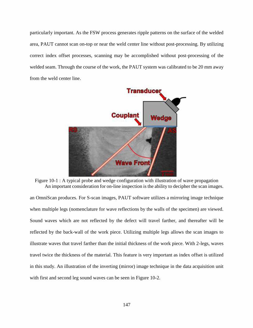
147

particularly important. As the FSW process generates ripple patterns on the surface of the welded

area, PAUT cannot scan on-top or near the weld center line without post-processing. By utilizing

correct index offset processes, scanning may be accomplished without post-processing of the

welded seam. Through the course of the work, the PAUT system was calibrated to be 20 mm away

from the weld center line.

Figure 10-1 : A typical probe and wedge configuration with illustration of wave propagation

An important consideration for on-line inspection is the ability to decipher the scan images.

an OmniScan produces. For S-scan images, PAUT software utilizes a mirroring image technique

when multiple legs (nomenclature for wave reflections by the walls of the specimen) are viewed.

Sound waves which are not reflected by the defect will travel farther, and thereafter will be

reflected by the back-wall of the work piece. Utilizing multiple legs allows the scan images to

illustrate waves that travel farther than the initial thickness of the work piece. With 2-legs, waves

travel twice the thickness of the material. This feature is very important as index offset is utilized

in this study. An illustration of the inverting (mirror) image technique in the data acquisition unit

with first and second leg sound waves can be seen in Figure 10-2.

148

Figure 10-2 : (a) PAUT S-scan Image displaying the effect of SDH at larger depth, with

associated schematic of first and second legs with SDH defect (b).

It can be seen that the initial defect image is at a depth of 7.3 mm in Figure 10-2(a). An

apparent second defect at a distance of 9.4 mm is also observed. The second defect image is located

at a distance that exceeds the thickness of the work piece (8.32 mm thickness for this experiment).

The defect’s actual depth is evaluated by the operator taking the difference of the depth given from

the image and work piece thickness. The resulting value is then subtracted from the work piece

thickness, which is the location similar to the first leg defect depth. In summary, due to the many

elements in a PAUT transducer, signals emitted from certain elements may not be influenced by a

defect; consequently, the first leg signals from those elements have not been redirected. These

signals are then reflected off the bottom surface of the specimen which re-directs the signal that

results in reflecting off the defect. This is illustrated in Figure 10-2(b) for the defect at the larger

depth.

149

10.3. PAUT vs. X-Ray Radiography for Post-Weld Inspection

A comparison of the abilities of PAUT and X-ray radiography to detect various forms and

sizes of defects in weldments has been carried out in this study. The FS welded plates were

analyzed employing PAUT and compared with X-ray radiography to illustrate sizing capabilities

when utilizing a calibrated PAUT system (note the x-ray images below are inverted for better

quality). These FS welds were executed utilizing varying weld schedule parameters (plunge or

forge force, feedrate, and spindle rotational speed). Weld schedules were designed in a way to

purposely produce defects. Four defect types are presented below. Defects presented in this study

include surface cavities (SC), wormhole (WH), internal voids (IV), and incomplete penetration

(IP). SCs are surface defects whereas WH and IV are internal defects. IP is a defect located at the

root of a weld caused by unconsolidated material on the seam line. Each defect type has a different

formation mechanism and are directly related to the process parameters utilized during welding.

Firstly, a SC formed by lack of material in the weld seam during plunge stage of a FSW is

presented. Secondly a WH defect is presented followed by another SC, often considered a

trenching (TR) defect, is shown. Thereafter, an IV is shown. Lastly, IP defects are described. In

FSW, typical defect locations of each defect can be observed in Figure 10-3 with anticipated legs

which will find the defects.

Figure 10-3 : Illustration of PAUT system with various legs indicating where FSW defects may

occur.

150

Figure 10-4 illustrates a FS weld that has incurred a large defect located on the AS of the

weld. A-scan image can be seen with associated S-scan image. The S-scan image depicts a

snapshot of the defect with accurate estimates of its size and location. It is observed that the defect

is found by second leg signals, as the depth of the defect is greater than the workpiece thickness,

i.e., 8.32 mm, and less than doubled thickness, i.e., 16.64 mm. Figure 10-5 illustrates a

representation of the X-ray image compared with B-scan and C-scan of the PAUT system.

Furthermore, in Figure 10-6 and Figure 10-7 a WH defect is shown. In a similar fashion, a SC

defect is presented in Figure 10-8 and Figure 10-9. These defects were as well detected by the

second leg signals, as the wedge/transducer system is not scanning near or on-top of the defect. In

Figure 10-6, it is noted that the WH was also found by third leg signals, as the defects depth is

greater than 16.64 and less than 24.96 mm. It can be seen that as the signal propagates further

through the specimen, the defect depth has larger error. These defects were found accurately with

X-ray radiography and PAUT. Note there was no post-processing of the panels for these tests. The

X-ray image compares very well with PAUT scans and shows that the two NDE techniques

correlate very well for large defects, which is expected; however, it can be said that defects of this

size and shape will most likely not occur in the production line.

Figure 10-4 : Optical image of cross-section, enlarged defect image, PAUT A-Scan and S-Scan

image (second leg) of FS welded panel with surface cavity (Observed by Second Leg).

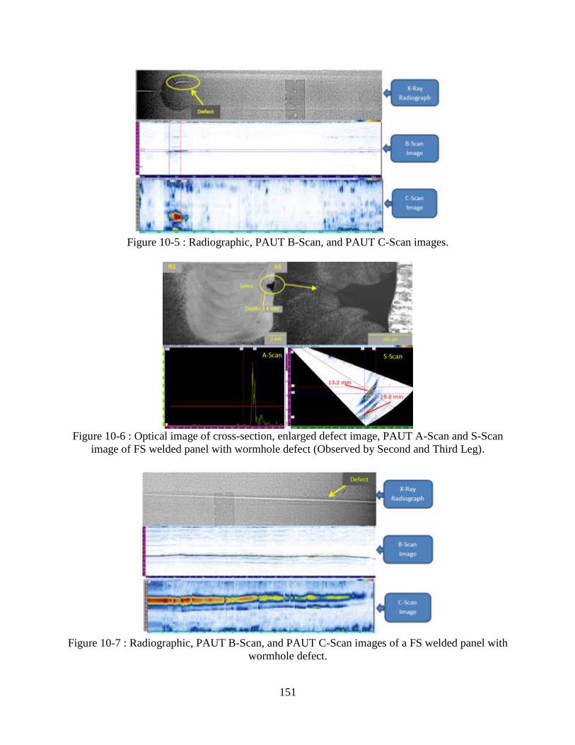
151

Figure 10-5 : Radiographic, PAUT B-Scan, and PAUT C-Scan images.


image of FS welded panel with wormhole defect (Observed by Second and Third Leg).

Figure 10-7 : Radiographic, PAUT B-Scan, and PAUT C-Scan images of a FS welded panel with

wormhole defect.

152


image of FS welded panel with SC defect (Observed by Second Leg).

Figure 10-9 : Radiographic, PAUT B-Scan, and PAUT C-Scan images of a FS welded panel with

SC defect.

An internal void defect is shown below in Figure 10-10 and Figure 10-11. In this FS weld,

two defects were found by the PAUT system; however, both defects were not found by x-ray

radiography. The smaller defect on the right in Figure 10-11 is analyzed here. The defect was

measured to be in the range of 0.15 mm in length and height. It is seen that the A-scan amplitude

does not reach 80% due to calibrating the system with a larger defect size. The intensity of the

reflected sound wave decreased giving maximum amplitude of ≈ 68%. It is observed that the X-

ray image does not detect the small defect.

153


image of FS welded panel with internal void (Observed by Second Leg).

Figure 10-11 : Radiographic image, PAUT B-Scan image, and C-Scan image of FSW panel with

internal void.

One challenging defect for NDE techniques to observe is IP. As this defect can be

detrimental for industrial applications, many studies have analyzed said defects for all major

welding processes; however, few pertaining to IP for FSW by employing ultrasonic techniques

can be found in the open literature. Lamarre et at. [256] employed a triple NDT approach including

ultrasonic pulse echoes, ultrasonic attenuation measurements, and eddy currents to analyze FS

welded specimens. It is stated that the triple NDT technique detects FSW defects including KBs

(IP defects). Alternatively, it was shown that ultrasonic C-scan images are difficult to observe IP;

however, utilizing a noise ratio of parent and weld material a better indication of IP can be

154

obtained. A high noise ratio indicates a kissing bond is present. Mandache et al. [247] compared

multiple NDE techniques (pulsed eddy current, conventional eddy current, PAUT, laser generated

ultrasonic waves with synthetic aperture focusing technique (SAFT), liquid die penetrant) to

analyze IP defects where a retractable pin tool was employed to vary the depth of penetration on a

2.56 mm thick panel. Employing a 10 MHz-16 element probe, it was possible to detect IP defects

with lengths greater than 0.2 mm from the root of the weld. In their study however, post-processing

of FS welded specimens was conducted, whereas in our study no post-processing was carried out

in order to correlate with on-line scanning. Bird et al. [257] developed a method to determine the

forging depth of FS welds by material noise ratio analysis which was able to measure penetration

better than 0.5 mm. Furthermore, in that study it was stated that employing ultrasonic amplitude

rejection for conventional defects, it was possible to discover voids with a through wall size of 0.1

mm. A study by the same research group of the previous study developed statistical signal

processing algorithms [258] which have the ability to identify weld nugget and root. Laser

ultrasonics composed of a Nd:YAG laser in conjunction with a photorefractive interferometer was

employed in [259] to detect internal defects and residual stresses. It was shown that such system

can detect IP defects as well.

Throughout the FS experimental program carried out in our research multiple IP defects

were found, as can be seen in Table 10-1. In the present study X-ray radiography had difficulty in

detecting IP defects. Alternatively, PAUT was able to discover IP defects; however, an increase in

gain value was needed in order to provide A-scan signal peak amplitude values near acceptable

limits with the aforementioned calibration, which originally allowed 80% A-scan peak amplitude

for 0.79 mm defects. Even with the increase in gain, the signal to noise ratio of the system was still

adequate to accurately observe defects. Few IP defects could not be discovered by the PAUT

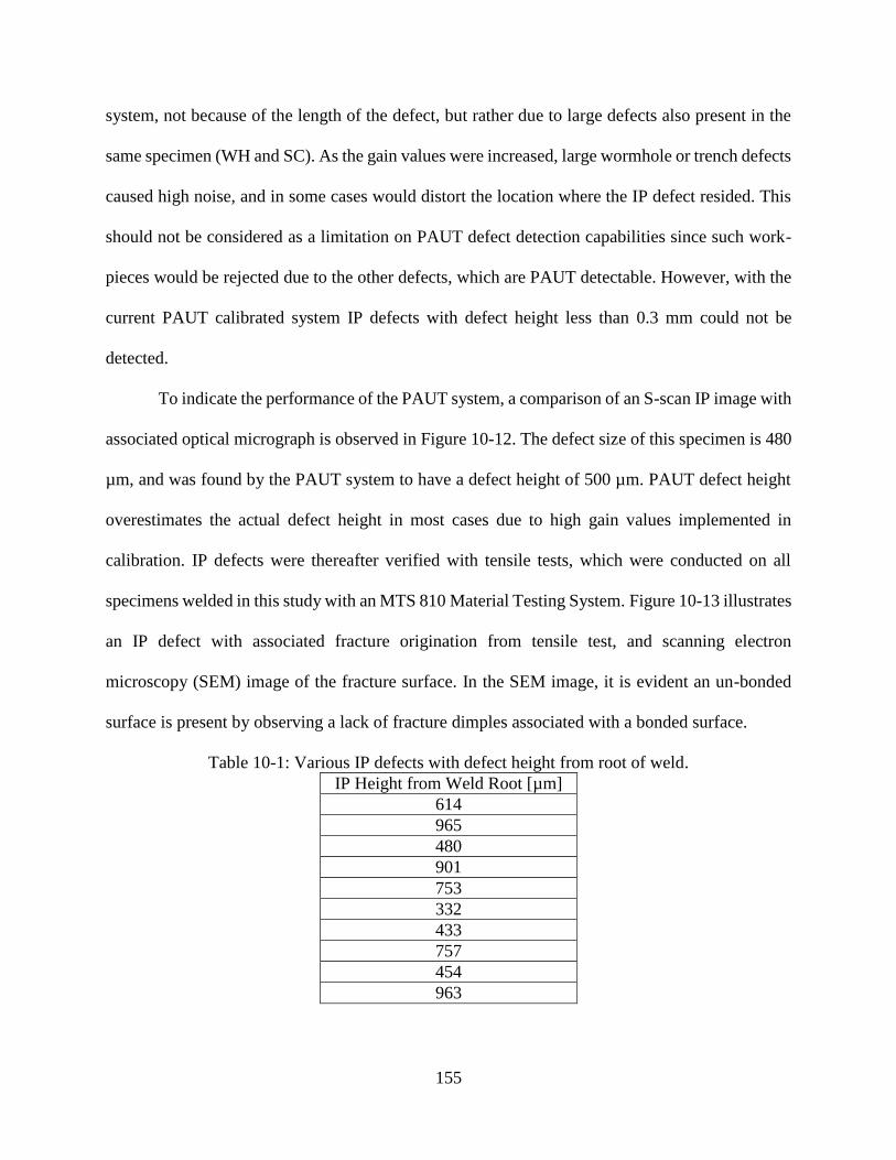
155

system, not because of the length of the defect, but rather due to large defects also present in the

same specimen (WH and SC). As the gain values were increased, large wormhole or trench defects

caused high noise, and in some cases would distort the location where the IP defect resided. This

should not be considered as a limitation on PAUT defect detection capabilities since such work-

pieces would be rejected due to the other defects, which are PAUT detectable. However, with the

current PAUT calibrated system IP defects with defect height less than 0.3 mm could not be

detected.

To indicate the performance of the PAUT system, a comparison of an S-scan IP image with

associated optical micrograph is observed in Figure 10-12. The defect size of this specimen is 480

µm, and was found by the PAUT system to have a defect height of 500 µm. PAUT defect height

overestimates the actual defect height in most cases due to high gain values implemented in

calibration. IP defects were thereafter verified with tensile tests, which were conducted on all

specimens welded in this study with an MTS 810 Material Testing System. Figure 10-13 illustrates

an IP defect with associated fracture origination from tensile test, and scanning electron

microscopy (SEM) image of the fracture surface. In the SEM image, it is evident an un-bonded

surface is present by observing a lack of fracture dimples associated with a bonded surface.

Table 10-1: Various IP defects with defect height from root of weld.

IP Height from Weld Root [µm]

614

965

480

901

753

332

433

757

454

963

156

Figure 10-12 : Optical image (left) of IP defect of length 480 µm and associated S-scan image

(right) of IP defect.

Figure 10-13 : A) Optical micrograph of IP defect, B) Optical image of tensile tested specimen

indicating fracture origination; C) SEM image indicating un-bonded area.

157

10.4. On-line PAUT

The ultimate goal of this study is to develop an online PAUT system that can detect various

FSW associated defects in real-time, thus expediting the inspection process and any remedy

measures that need to be taken such as adjusting weld schedules. There are many challenges in the

path to developing such an online system. This section addresses major challenges that were

investigated as part of this study; namely, high temperature and geometric constraints due to weld

fixtures. Finally, a demonstration of the proposed system is presented for some preliminary welds.

10.4.1 High Temperature Ultrasonics

HT studies on material velocity effects for PAUT on AAs for practical applications are, to

the authors’ knowledge, not readily available in open literature. Presented here is a review of the

few works that have been obtained. An early investigation of steels at high temperatures was

conducted in Ref. [260] utilizing conventional ultrasonic techniques. At 400°C a system was

created to mount piezoelectric arrays on steel in an industrial plant. It is stated that the system

effectively detected 1 mm side drilled holes at room temperature and 400°C. Subbaratnam et al.

[261] investigated ultrasonic time of flight diffraction (TOFD) in austenitic stainless steel. TOFD

tests evaluated at 149.85°C resulted in degradation of ultrasonic signals which was compensated

with an increase in gain values above what was required at ambient conditions. Similar trends were

observed in Johnson et al. [262], in which various AA’s (AA-1100, AA-2024-T351, AA-6061-T6,

AA-7075-T6) longitudinal ultrasonic velocities were measured as temperature of the specimens

was increased to solidus temperature. The work employed a Nd:YAG laser with pulses of 15 ns

with energy 700 mJ to excite ultrasonic waves. It is stated that at high temperatures (approximately

greater than 400°C) linear temperature dependence deviates. Development towards creating a

flexible transducer array at 150°C was conducted in Ref. [263]. A study by Tariq et al. [264]

158

examined various AAs including AA-2219 which illuminated that ultrasonic testing can be

conducted to correlate hardness values to material velocity and attenuation. The study states that

the material velocity of AA-2219 with a hardness (HV) of 138 correlates with a longitudinal

velocity, with a 4 MHz probe, of 6.354 mm/µs.

Employing the knowledge gained from the post-weld FSW analysis, a method to

incorporate FSW working conditions was employed for real time PAUT scanning. Firstly, PAUT

transducers are quite sensitive to heat. Typically the elements in a transducer are warranty rated

by the manufacturer from 5°C to 45°C. This is a leading cause why PAUT is seldom employed for

high temperature (HT) applications. Consequently, as mentioned in the literature a change in

temperature will cause a change in the ultrasonic velocity which poses issues for accurate defect

detection. For this reason, experiments were conducted to determine approximate temperature

ranges near the weld seam during FSW tests. K-type thermocouples and infrared imaging

techniques were employed and determined a maximum temperature of 312°C was reached 20 mm

away from the weld seam for the welding configuration. Consequently, to circumvent these high

temperatures in order to prevent damage to the sensitive piezoelectric elements a wedge was

designed by the authors and fabricated from vespel material (temperature rated: 287.8°C constant

to 482.2°C intermittent) by Sonatest. As this material is rated near the eutectic melting temperature

of binary aluminum-copper alloys (548°C [93]), this material was deemed suitable for the FSW

application. The wedge was further designed with a water inlet and outlet for cooling around the

transducer casing to ensure piezoelectric element safety. Furthermore, inlets were inserted to allow

a steady flow of couplant to the workpiece during scanning, see Figure 10-14.

The effectiveness of the newly designed and fabricated wedge was first tested in a

laboratory setting for a simulated controlled environment at ambient and elevated temperatures

159

(25.0°C, 100°C, 200°C, and 300°C). The experiments entailed three trials per temperature, and

utilized a different calibration file for east trial. Temperature readings were taken with K-type

thermocouples and Midi Logger GL820 acquisition system with a sampling rate of 200 ms. A

Thermo-Scientific 2200 Hot Plate was employed to heat the AA-2219-T87 material used for

calibration. In order to pump coolant and couplant through the wedge by the inlets and outlet

channel, two Master-Flex pumps were employed. Couplant is required to induce transmission of

ultrasonic waves from wedge to workpiece, and the coolant is required to maintain a safe operating

temperature for the piezoelectric elements in the transducer. Figure 10-15 illustrates the

experimental setup.

Figure 10-14 : Custom PAUT HT wedge/transducer unit.

Figure 10-15 : Illustration of HT PAUT for SDH AA-2219 specimen of 8.13 mm thickness.

160

Table 10-2 summarizes the experimental results at ambient conditions. It is observed that

with appropriate calibration procedures accurate defect sizing and location was obtained, similar

to conventional PAUT wedges. The effects at elevated temperatures can be seen in Table 10-3.

Figure 10-16 illustrates two S-scan images of a similar defect at varying temperatures (ambient

and 300°C). It was observed that the location of the defect increased in distance as the temperature

increased, due to the change in ultrasonic velocity as the material heats. It is observed that at 300°C

the maximum depth change was found to be 1.2 mm. This value appears small, and indicates that

at 300°C there is minimal change for our PAUT configuration. One reason for this small change

is due to the unconventional wedge material that is utilized. According to ASME standard [265]

high-temperature materials up to 540°C can be measured with appropriate HT instruments. For

steel, it is claimed the rule of thumb for apparent thickness measurements with elevated

temperatures increases by a factor of 1% per 55°C. A comparison of defect depth variation with

temperature can be seen in Figure 10-17. At room temperature, error in depth measurement is

small compared to when an increase in temperature occurs. With an increase in temperature, defect

depth increases. Defect depth measurement variation also increases when the temperature and

defect location increases. Furthermore, the attenuation has increased at higher temperatures, which

can be observed by the reduction in A-scan peak amplitude. At room temperature 80% A-scan

peak amplitude (as calibrated) is obtained whereas at 300°C a decrease in A-scan peak amplitude

is obtained; consequently, the gain value should be increased to compensate for the loss in signal

intensity. When a material’s temperature increases, the atoms inside are in an elevated energy state

which increases interatomic spacing which impedes transmission. Consequently, at these

temperatures a calibration of the software must take place in order to compensate for these high

temperatures with a change in material velocity. To improve this study, and to devise appropriate

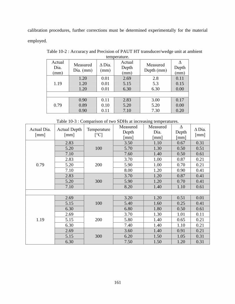
161

calibration procedures, further corrections must be determined experimentally for the material

employed.

Table 10-2 : Accuracy and Precision of PAUT HT transducer/wedge unit at ambient

temperature.

Actual

Dia.

(mm)

Measured

Dia. (mm)

Δ Dia.

(mm)

Actual

Depth

(mm)

Measured

Depth (mm)

Δ

Depth

(mm)

1.19

1.20 0.01 2.69 2.8 0.11

1.20 0.01 5.15 5.3 0.15

1.20 0.01 6.30 6.30 0.00

0.79

0.90 0.11 2.83 3.00 0.17

0.89 0.10 5.20 5.20 0.00

0.90 0.11 7.10 7.30 0.20

Table 10-3 : Comparison of two SDHs at increasing temperatures.

Actual Dia.

[mm]

Actual Depth

[mm]

Temperature

[°C]

Measured

Depth

[mm]

Measured

Dia.

[mm]

Δ

Depth

[mm]

Δ Dia.

[mm]

0.79

2.83

100

3.50 1.10 0.67 0.31

5.20 5.70 1.30 0.50 0.51

7.10 7.60 1.40 0.50 0.61

2.83

200

3.70 1.00 0.87 0.21

5.20 5.90 1.00 0.70 0.21

7.10 8.00 1.20 0.90 0.41

2.83

300

3.70 1.20 0.87 0.41

5.20 5.90 1.20 0.70 0.41

7.10 8.20 1.40 1.10 0.61

1.19

2.69

100

3.20 1.20 0.51 0.01

5.15 5.40 1.60 0.25 0.41

6.30 6.80 1.80 0.50 0.61

2.69

200

3.70 1.30 1.01 0.11

5.15 5.80 1.40 0.65 0.21

6.30 7.40 1.40 1.10 0.21

2.69

300

3.60 1.40 0.91 0.21

5.15 6.20 1.50 1.05 0.31

6.30 7.50 1.50 1.20 0.31

162

Figure 10-16 : Comparison of A- and S-scan images of 1.19 mm diameter SDH at a depth of 6.3

mm. Case A) conducted at room temperature, and case B) conducted at 300°C. A change in

depth of 1.2 mm occurred with an increase in temperature to 300°C with an increase in

attenuation (80% down to 64% A-scan peak amplitude).

Figure 10-17 : Effect of temperature on defect measurement for HT PAUT system for SDH of

diameter 0.79 mm (top) and 1.19 mm (bottom).

10.4.2 FSW Fixture

A FSW fixture is a key factor in determining weld quality. The fixture rigidly holds the

material to be welded in place and also acts as a heat sink. In order for the development of an on-

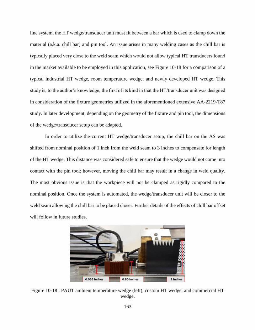
163

line system, the HT wedge/transducer unit must fit between a bar which is used to clamp down the

material (a.k.a. chill bar) and pin tool. An issue arises in many welding cases as the chill bar is

typically placed very close to the weld seam which would not allow typical HT transducers found

in the market available to be employed in this application, see Figure 10-18 for a comparison of a

typical industrial HT wedge, room temperature wedge, and newly developed HT wedge. This

study is, to the author’s knowledge, the first of its kind in that the HT/transducer unit was designed

in consideration of the fixture geometries utilized in the aforementioned extensive AA-2219-T87

study. In later development, depending on the geometry of the fixture and pin tool, the dimensions

of the wedge/transducer setup can be adapted.

In order to utilize the current HT wedge/transducer setup, the chill bar on the AS was

shifted from nominal position of 1 inch from the weld seam to 3 inches to compensate for length

of the HT wedge. This distance was considered safe to ensure that the wedge would not come into

contact with the pin tool; however, moving the chill bar may result in a change in weld quality.

The most obvious issue is that the workpiece will not be clamped as rigidly compared to the

nominal position. Once the system is automated, the wedge/transducer unit will be closer to the

weld seam allowing the chill bar to be placed closer. Further details of the effects of chill bar offset

will follow in future studies.

Figure 10-18 : PAUT ambient temperature wedge (left), custom HT wedge, and commercial HT

wedge.

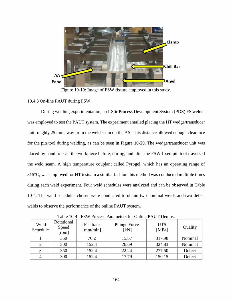
164

Figure 10-19: Image of FSW fixture employed in this study.

10.4.3 On-line PAUT during FSW

During welding experimentation, an I-Stir Process Development System (PDS) FS welder

was employed to test the PAUT system. The experiment entailed placing the HT wedge/transducer

unit roughly 25 mm away from the weld seam on the AS. This distance allowed enough clearance

for the pin tool during welding, as can be seen in Figure 10-20. The wedge/transducer unit was

placed by hand to scan the workpiece before, during, and after the FSW fixed pin tool traversed

the weld seam. A high temperature couplant called Pyrogel, which has an operating range of

315°C, was employed for HT tests. In a similar fashion this method was conducted multiple times

during each weld experiment. Four weld schedules were analyzed and can be observed in Table

10-4. The weld schedules chosen were conducted to obtain two nominal welds and two defect

welds to observe the performance of the online PAUT system.

Table 10-4 : FSW Process Parameters for Online PAUT Demos.

Weld

Schedule

Rotational

Speed

[rpm]

Feedrate

[mm/min]

Plunge Force

[kN]

UTS

[MPa] Quality

1 350 76.2 15.57 317.98 Nominal

2 300 152.4 26.69 324.83 Nominal

3 350 152.4 22.24 277.50 Defect

4 300 152.4 17.79 150.15 Defect

165

Figure 10-20 : Custom PAUT HT wedge/transducer unit scanning during FSW.

The above experiments confirmed that the PAUT HT wedge/transducer unit performed well. The

wedge/transducer was able to assess the weld seam in the high temperature environment. Due to

the position of the wedge/transducer and butt-joint configuration, before the pin tool passed the

scanning area to make the weld a large defect is signaled by the PAUT system due to the un-

welded seam. The high frequency waves reflecting off the wall have the appearance of a large

defect. For the defect free experiments, once the pin tool traversed the weld seam material was

consolidated providing no defect signals. However, when defects are welded into the workpiece

the PAUT system is able to capture them. Figure 10-21 illustrates the S-scan images of the un-

welded seam, nominal weld without defect, and weld with defect. As discussed previously,

multiple legs are employed to scan the entire welded area. Consequently, care must be applied in

interpreting the results as the distance for scanning in these experiments employed three legs,

which can have adverse effects on correctly interpreting defect signals.

In image (c) of Figure 10-21, only signals generated at large angles could determine the

defect due to the distance the probe was placed from the weld seam, as indicated by Figure 10-22.

Here the first defect image was found by the second leg, and thereafter the second defect image

was found by the third leg. The back-wall was not found in image shown in Figure 10-21(b) due

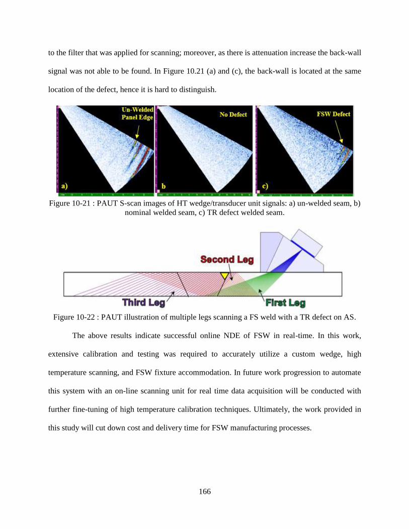
166

to the filter that was applied for scanning; moreover, as there is attenuation increase the back-wall

signal was not able to be found. In Figure 10.21 (a) and (c), the back-wall is located at the same

location of the defect, hence it is hard to distinguish.

Figure 10-21 : PAUT S-scan images of HT wedge/transducer unit signals: a) un-welded seam, b)

nominal welded seam, c) TR defect welded seam.

Figure 10-22 : PAUT illustration of multiple legs scanning a FS weld with a TR defect on AS.

The above results indicate successful online NDE of FSW in real-time. In this work,

extensive calibration and testing was required to accurately utilize a custom wedge, high

temperature scanning, and FSW fixture accommodation. In future work progression to automate

this system with an on-line scanning unit for real time data acquisition will be conducted with

further fine-tuning of high temperature calibration techniques. Ultimately, the work provided in

this study will cut down cost and delivery time for FSW manufacturing processes.

167

10.5. Conclusions

This chapter presented a systematic study of PAUT for both post-weld and online

inspection. Moreover, the capability of PAUT in detecting various forms of defective FS welds

has been investigated and compared with X-ray radiography. One of the objectives of this study

was to increase understanding of post-weld inspection with PAUT on FS welded specimens.

PAUT inspection is complex and requires significant time and understanding in order to be applied

effectively. For these reasons, and due to a lack of literature of current PAUT methods on FS

welds, a necessary study was conducted to illustrate the subtleties of PAUT operation with respect

to the FSW technique. As the newly developed FSW process expands in industry, post-weld

inspection will be heavily relied upon. It has been shown that the PAUT technique is an excellent

choice for this undertaking and also more reliable than X-ray radiography. The importance of A-

scan amplitude, index offset, TCG calibration, PAUT image analysis, and defect sizing were

discussed. Furthermore, IP defects can be detrimental to aerospace industries as they are difficult

to detect with PAUT and X-ray radiographic NDE techniques. IP defects are able to be discovered

with increase in gain compared to the system calibrated for typical scanning procedures.

Furthermore, successful implementation of a wedge/transducer unit for high temperature

application has been shown. With an increase in temperature, PAUT software calibration is

required to compensate for material property changes. For the first time, PAUT has been applied

real time during FSW.

As the work progresses, an on-line scanning system will be developed and employed to

automate NDE sensing of FSW which will greatly aid manufacturing processes. Another study

will attempt to correlate welding schedules with defects for the purpose of predicting whether a

168

defective weld will be produced for a certain welding setting and determining optimal friction stir

welding conditions.

169

CHAPTER 11 : ON-LINE HIGH TEMPERATURE PHASED ARRAY

ULTRASONIC INSPECTION OF FIXED PIN FRICTION STIR WELDS

AND ITS IMPACT ON WELD QUALITY

Every honest researcher I know admits he's just a professional amateur. He's doing whatever he's

doing for the first time. That makes him an amateur. He has sense enough to know that he's

going to have a lot of trouble, so that makes him a professional.

-Charles Franklin Kettering

11.1. Introduction

Phased array ultrasonic testing (PAUT) has developed into a refined technique for weld

inspection. Unlike conventional ultrasonic testing (UT), PAUT offers the ability to inspect welds

at multiple angles with a single probe. PAUT has proven to be a versatile technique to evaluate

weld defects without causing damage to the part or rendering the workplace inoperable due to

hazardous conditions.

A specific welding technique that PAUT has been applied to in industry and academic

research is friction stir welding (FSW). FSW, a thermomechanical, grain refining, solid-state

process, is a reliable joining technique that has proven to obtain consistent high strength properties.

This is evident in the aerospace industry where FSW is employed for space vehicle fabrication.

NASA employs FSW for constructing their Orion crew module and Space Launch System (SLS)

core stage propellant tankage. Other entities such as United Launch Alliance (ULA), SpaceX, and

Blue Origin have also implemented FSW in construction of their rocket systems [3-5].

PAUT is capable to determine the different defects characteristic of FSW. PAUT is utilized

frequently to the extent that codes and standards have been produced to dictate operating

procedures as observed in ASTM E2700-14. In academic research, PAUT has been tested to

observe its capabilities as seen in [69, 247, 256, 257, 266-270]. In refs. [69, 256, 268, 269], PAUT

was found to perform well when inspecting volumetric defects in FS welds. In refs. [257, 270], the

authors identify PAUT’s capability to find challenging defects such as joint line remnants (JLR)

170

and entrapped oxide defects. Utilizing techniques of ultrasonic signal ratio analysis and amplitude

rejection it was possible to discover defects. In another study, the incomplete penetration (IP)

defect was investigated [247]. In that study it is indicated that PAUT can detect IP corresponding

to a length of 0.2 mm; however, it was observed that the kissing bond defect was not able to be

discovered due to the defect’s orientation. Ref. [266] evaluated the capabilities of several NDT

techniques and identified that PAUT was best suited for automated NDE processes, and will

ultimately replace manual NDE techniques. PAUT was also able to identify interface defects in a

hybrid lap joint study in ref. [267].

In industry, welded components for FSW are typically large which postures difficulties to

non-destructively test in a timely manner. On-line PAUT inspection during the welding process

would be the most economical practice; however, this is not conducted as high temperatures (HTs)

during welding can damage PAUT transducers. FSW also poses geometric limitations due to

workpiece fixturing which limits space for PAUT units. For this reason, methods to evaluate FS

welds at HTs on-line during the weld process is developed in this work to aid manufacturing

efficiency.

The main focus of the research in the literature listed previously aimed to create methods

to implement PAUT on FS welded structures off-line and identify specific defect types. The work

in this chapter differs from those as the aim here is to create a new application for PAUT and

incorporate the process for real-time inspection. This study also provides the framework for HT-

PAUT inspection utilizing two varying scanner system designs. Furthermore, the impact that the

HT-PAUT systems have on joint quality and microstructure are identified which can aid in paving

the future development for on-line HT-PAUT systems.

171

The remaining sections in this chapter are organized as follows: Section 11.2 illustrates the

experimental conditions employed in this work. In Section 11.3, the development of a custom HT-

PAUT wedge-transducer unit is presented and HT-PAUT features are discussed. Furthermore, two

varying on-line HT-PAUT scanning systems are presented illustrating the capabilities of each.

Section 11.4 provides defects observed on-line during the welding process. Thereafter, the impact

the PAUT on-line scanning systems have on microstructure is presented and identification of pros

and cons of each scanning system is discussed in Section 11.4. The last section concludes the work.

11.2. Experimental Conditions

Welded specimens in this work were fabricated at the NASA Michoud Assembly Facility

(MAF) in New Orleans, Louisiana [34, 121, 201, 229]. MAF houses the National Center for

Advanced Manufacturing (NCAM) which contains state-of-the-art FSW machines including

Process Development System (PDS) and Universal Weld System (UWS) platforms. In this work,

the PDS platform was employed only compared to the work in the other chapters. The material

employed included AA-2219-T87 panels with dimensions 609.6 mm long, 152.4 mm wide and

8.13 mm thick. Two panels were welded in a typical butt-joint configuration with a fixture that

utilized a steel anvil. Steel bars were placed on the advancing side (AS) and retreating side (RS)

38.1 mm away from weld centerline and each held in place with four clamps. Side compression

screws were used on the RS. Before welding, the panels were lightly ground to remove the oxide

layer and wiped with an alcohol solution. The welds employed a 0° lead angle with zero index-

offset from the centerline, and joined with a two-piece fixed pin tool. The pin tool’s shoulder,

made from H13 steel, has a 30.48 mm diameter with 0.76 mm deep counter clockwise (CCW)

spiral scroll of 2.92 mm pitch. The pin, which is interchangeable, is an MP159 cone of 10.16 mm

diameter at shoulder with 18 TPI UNC LH threads of length 7.11 mm. The pin has a 10° taper

172

angle. The experimental setup can be observed in Figure 11-1 with the welding system and pin

tool.

Figure 11-1: A) Fixed pin tool and B) I-Stir PDS machine employed in this study, and C) the

FSW process during experimentation at the NASA Michoud Assembly Facility.

The welded joints were tested during and after welding with PAUT. PAUT instrumentation

included an Olympus OMNIScan MX2 system with a 5 MHz – 32 element transducer. The

couplant employed during testing was the HT rated Pyrogel grade 7. Welded joints were thereafter

sectioned with a metal-cutting saw into tensile and macrograph coupons. These coupons were

destructively tested in tension with an MTS 810 Material Test System. Sectioned coupons were

polished to 0.05 microns and etched with Keller’s reagent and inspected via optical techniques.

11.3. Design of Two On-Line HT-PAUT FSW Systems

11.3.1. HT-PAUT Considerations

The work in this Chapter builds upon knowledge gained from refs. [121, 229]. In ref. [121],

the methods to evaluate FS welded structures were determined. It was observed that at HTs sound

173

velocity in the wedge and components vary which affects focal law calculations that can lead to

positioning errors when locating defects. Ultrasonic signal attenuation is another factor that is

required to account for during operation, and thus a proper time corrected gain (TCG) calibration

must be conducted. An outcome of that work was the development of a custom HT wedge made

from vespel which has an operating range of 350°C. The custom wedge was designed to be small

and versatile to accommodate FSW fixtures. Furthermore, the couplant employed in that study

(Pyrogel grade 7) had an operating temperature of 315°C and was found to be suitable for the FSW

application.

In the literature, there are few efforts that pertain to HT-PAUT. The Olympus Corporation

has developed an HT wedge that can withstand temperatures in the range of 150°C [271]. In that

study an amorphous thermoplastic polyetherimide resin called ULTEM™ was employed. It was

determined that probes with frequencies over 5 MHz should not be used with ULTEM wedges due

to the center frequency shift. Another HT-PAUT study by EclipseScientific inspected defects at

temperatures up to 350°C [272]. In that work an algorithm was developed to correct focal law

element time delays for inspection at temperatures with shear planar waves. Another company

named TUVRheinland has stated that they can detect defects with PAUT at temperatures in the

range of 400°C; however, little details are available most likely due to its proprietary nature [273].

The HT wedge system developed here differs from the aforementioned works as our application

is to inspect FSW defects on-line, which to the author’s knowledge has not been conducted.

Furthermore, the required operating temperatures are required to be greater than 150°C, and also

needs the profile of the wedge/transducer unit to be minimal which is why a custom system was

developed.

174

11.3.2. On-Line Sensing System Designs

After developing the HT-PAUT capabilities for FSW, an automated system that could

inspect FSW joints during the weld process was developed. This was accomplished by

constructing a system that can attach the HT-PAUT unit to the PDS welding platform as observed

in [229]. In that study, a scanning system was designed and tested with 9 varying weld schedules

where defects were able to be detected. The first design, titled On-Line Scanner System #1 (OLSS-

1), entailed mounting the HT-PAUT unit to a bracket that connects to the FS welder. The scanner

system was designed to be fastened to the welder’s adapter rings that are positioned above the tool

shoulder adapter and casing. Connecting the scanning system to the weld machine allows

versatility by utilizing the weld system to move the HT-PAUT unit. This feature eliminates travel

speed calibrations and will ensure that the HT-PAUT unit will have a constant scanning distance

relative to the pin tool.

OLSS-1 utilizes a spring loaded system to compensate for the distance that the weld head

travels in the downward direction, which also acts as the mechanism to keep the wedge in intimate

contact with the workpiece surface. OLSS-1 incorporates multiple degrees of freedom to

compensate for changes in the pin tool design or shoulder adapter geometry. The OLSS-1 can be

grouped into four subassemblies that include mounting, adjustment, sliding, and transducer/wedge

as observed in Figure 11-2.

While in operation, the on-line scanner system allows the HT-PAUT unit the ability to

transmit ultrasonic waves behind the pin tool after the faying surfaces of the workpieces are joined.

Although, placing the HT-PAUT unit behind the pin tool causes an issue with the build-up of

material at the start of the weld during the plunge phase for fixed pin FSW. To circumvent the HT-

PAUT unit from riding over this material, a sliding mechanism was designed so the HT-PAUT

175

unit could be placed before the weld head (Sliding Subassembly). As the weld head moves to the

distance that the HT-PAUT unit requires for scanning, a stopper pushes the unit in tandem with

the weld head.

Figure 11-2: OLSS-1 design illustrating the 4 subassemblies of the system (left) and the OLSS-1

attached to the PDS FS welder at the NASA Michoud Assembly Facility (right).

During development, it was known that the created HT-wedge system would require an

adjustment to the FSW fixture. The adjustment to accommodate the OLSS-1 required the fixture’s

chill bar, the component of the fixture which acts as a heat sink and fastening system for the

workpieces, to be shifted roughly twice the distance away from the weld seam compared to

nominal conditions as observed in Figure 11-3. In Figure 11-3A, the nominal FSW fixture

configuration is shown where the chill bar is placed roughly 38.1 mm away from the joint center

line. In Figure 11-3B, the chill bar was required to be placed 65.2 mm away from the joint center

line to accommodate OLSS-1.

176

After development of OLSS-1, a second scanner system was developed to illustrate that

various scanner designs can be instituted to accommodate a HT-PAUT unit and illustrate the

adaptability of the HT-PAUT unit. The major differences in the design can be observed in the

mechanism which allows movement of the HT-PAUT unit with the PDS welder. OLSS-2 employs

a new mechanism based upon an alternative chill bar design to prevent the offset seen in OLSS-1,

and can be observed in Figure 11-3C. The chill bar for the OLSS-2 was designed to allow the HT-

PAUT unit to reside inside the chill bar, which prevents the HT-PAUT unit to be mechanically

fastened to the welder. In order to circumvent this an alternative method to fix the HT-PAUT unit

to the welder was established. The alternative method employs HT rated magnets that are fastened

to the HT-PAUT unit and a magnetic fastening subassembly that is attached to the PDS welder as

observed in Figure 11-4. The HT-PAUT unit subassembly utilizes two brackets that attach to the

HT-wedge which each hold one HT-magnet rated to 44.5 N maximum pull. The FSW magnetic

fastening subassembly holds another two HT-magnets which are rated to 71 N maximum pull.

Figure 11-3: Variation of FSW fixture employed during experimentation: A) Nominal FSW

fixture configuration, B) FSW fixture with chill bar offset, C) and FSW fixture with alternative

chill bar assembly.

177

Figure 11-4: OLSS-2 design illustrating the 4 subassemblies of the system. The hole cut-outs in

the magnetic fastening and HT-PAUT transducer/wedge subassemblies illustrate the locations

where HT magnetics are placed, which will act as the mechanism to move the wedge with the

friction stir welder.

In both scanner designs, the probe was placed on the AS of the weld. This was decided

based upon the fact that the majority of internal and surface defects in FS typically occur on the

AS. Placing the HT-PAUT unit on the AS allows the wedge to be closer to typical FSW defects

which provides better detection capabilities.

11.4. Defect Observations and HT-PAUT Impact on Microstructure

11.4.1. On-Line Detection of FSW Defects

In order to test both OLSSs, weld schedules were chosen to obtain defective joints that

include trenching (TR) and wormhole (WH) defects. The weld schedules utilized to test both

systems can be observed in Table 11-1. The schedules were based upon prior knowledge gained

from the works in refs. [34, 121, 229]. In those studies, a process parameter map was created based

178

upon an experimental FSW program where 90 weld schedules were conducted which resulted in

a process parameter map that employs plunge force on the ordinate and a pin speed ratio (PSR) on

the abscissa as seen in Figure 11-5. The PSR is the relationship 2𝜋𝑟∙𝜔

𝑉 where r is the pin tool’s

radius, ω is the spindle rotational speed, and V is the feedrate.

Table 11-1: Weld schedules conducted with both OLSSs to review performance of analyzing

defects.

OLSS ω

[RPM]

V

[mm/min]

Plunge Force

[kN] Defects

1 450 152.40 18.24-22.69 TR/WH

1 450 152.40 22.69-23.58 TR/WH

2 450 152.40 18.24-24.46 TR/WH

2 450 152.40 24.46-26.69 TR/WH

Figure 11-5: Process parameter map of weld schedules classified as hot, cold, and nominal

plotted with plunge force vs. PSR. The hot class of welds obtained small internal voids (IV) and

underfill/flash (UF/F) defects which exhibited a decrease in toughness. The cold class of welds

exhibited trenching (TR), wormholes (WHs), and incomplete penetration (IP) and lowest

mechanical properties. The nominal class indicates welds with no observable defects which

exhibit best strength and toughness.

During testing, the plunge force was varied to vary the size and location of defects. It was

observed that at low plunge forces large TR defects were obtained. As the plunge force was

increased, the TR defect’s thickness and width decreased. In several cases, the crown surface of

179

the weld consolidates successfully; however, just below the crown surface an internal cavity, or

wormhole (WH), formed. Increasing the plunge force further successfully consolidated the joint

with no defects.

The OLSSs were able to detect the defects obtained during experimentation. In Figure 11-6

the OLSS-1 can be observed during operation where a TR defect formed. Figure 11-6 also

illustrates a TR defect with associated A- and S-Scan images obtained from OLSS-1. In Figure

11-7 the OLSS-2 is shown during operation where a WH defect formed with associated A-and S-

Scan images.

Figure 11-6: OLSS-1 in operation during FSW discovering a TR defect (Top) with associated

PAUT A- (Bottom Left) and S-scan (Bottom Right) images.

180

Figure 11-7: OLSS-2 in operation during FSW discovering a WH defect (Top) with associated

PAUT A- (Bottom Left) and S-scan (Bottom Right) images.

The two systems illustrate that with an adequate scanning system, PAUT with HT

adjustments can detect defects on-line during the welding process. However, each system has its

strengths and weaknesses pertaining to providing the most suitable conditions for HT-PAUT.

OLSS-1 was found to allow the HT wedge to be placed closer to the weld seam which improves

signal attenuation and resolution characteristics. However, this causes the panel on the AS to have

clamping issues, which will be further discussed in the next section. On the other hand, OLSS-2

provided smoother conditions for the wedge to traverse along the weld seam. It was found that for

the OLSS-1 if the spring tension and wedge guide length was not optimized the wedge could skip

across the panel, momentarily losing defect detection capabilities. The powerful HT magnets of

the OLSS-2 allowed for stable scanning conditions which ensure reliable scans. OLSS-2 however

was found to have an increase in signal attenuation, or signal amplitude loss, as the HT-PAUT unit

was required to be placed farther away from the weld seam compared to OLSS-1. This is observed

181

in Figure 11-7 where the peak A-Scan amplitude was found to achieve only 68% for the largest

WH defect found. Similarly, low A-Scan amplitudes were observed when small TR defects were

present, and in some cases only reached 30% amplitude intensity.

11.4.2. On-Line HT-PAUT Weld Quality Impact

PAUT requires the deposition of couplant to transmit ultrasonic waves from the wedge to

the workpiece. Depositing couplant will act as a heat sink which may influence the microstructure

of the weld. Moreover, the change in chill bar configuration will vary weld quality as the clamping

conditions and thermal properties are altered. In order to determine these impacts on the current

FSW configuration, 4 weld schedules were conducted with nominal, OLSS-1, and OLSS-2

conditions. Weld schedules were chosen based upon the process parameter map in Figure 11-5,

and were chosen at 4 different PSRs where the plunge force was varied from 17.79 kN, 22.24 kN,

26.69 kN, and 31.14 kN as observed in Table 11-2.

Table 11-2: FSW weld schedules conducted with I-Stir PDS with associated defect

identification (DF - defect free, IP – Incomplete Penetration, Pl. Force – Plunge Force, Sch. –

Schedule, Tough. – Toughness, TR - Trenching defect).

Sch. ω

[RPM]

V

[mm/min] PSR

Pl.

Force

[kN]

Config. UTS

[MPa]

Tough.

[MJ/m³]

Avg.

SZ

Grain

Size

[µm]

Defects

1 300 228.60 41.89 31.14

Nominal 347.30 42.12 6.17 DF

OLSS #1 345.20 32.81 7.35 IP

OLSS #2 346.36 31.19 7.88 IP

2 400 203.20 62.83 26.69

Nominal 346.57 31.90 6.14 DF

OLSS #1 292.96 11.81 6.41 IP

OLSS #2 311.84 17.70 8.31 IP

3 300 101.60 94.25 22.24

Nominal 354.21 46.24 6.13 DF

OLSS #1 336.72 32.16 5.42 IP

OLSS #2 337.95 36.96 7.45 IP

4 400 101.60 125.6 17.79

Nominal 358.12 33.45 6.22 DF

OLSS #1 141.89 2.14 6.55 TR

OLSS #2 178.20 2.51 7.58 TR/WH

182

Table 11-2 identifies the mechanical properties of UTS and toughness for each weld

schedule with the associated average grain size in the stirred zone (SZ). It is observed in all cases

that the mechanical properties decreased when the OLSS conditions were employed compared to

nominal conditions. A major reason for the decrease in the mechanical properties is the formation

of IP, WH, and TR defects as observed in Figure 11-8. It was observed that schedule #4 obtained

the largest deviation in mechanical properties, where schedule #1 was observed to show the least

variation. Schedule #4 produced a severe TR defect with the OLSS-1 configuration whereas when

the OLSS-2 configuration was employed TR and WH defects were present. It is evident that

schedule #4 has the lowest tolerances for configuration variation compared to nominal conditions.

This leads to the conclusion that weld schedules with lower plunge forces lead to a decrease in

fixture variation; however, this is a general statement as these results could vary if the spindle

rotational speed and feedrate were also varied. Schedule #1 was observed to have incomplete

penetration at the root of the weld. During tensile testing, the unconsolidated material opened to

reveal the defect; however, the defect could not propagate further as material that was successfully

joined prevented total failure of the joint. The test continued until the specimen failed in the HAZ

with a near 45° shear failure as observed in Figure 11-9. This phenomenon occurred as well in

schedules #2 and #3; however, in those cases the fracture varied in few cases where propagation

occurred through the SZ on the AS. It is also illustrated that the ‘onion ring’ [173] layering of the

nominal configuration welds compared to the OLSS configurations vary indicating that the

eccentric pumping motion of the pin tool has changed. As FSW is a solid-state joining process

where the material in the SZ is both heated and deformed, this causes temperature-induced and

mechanically induced variations in structure which could cause differential polishing or etching

within the recrystallized weld nugget grain structure [274] as observed in Figure 11-8 .

183

Figure 11-8: Transverse cross-sections of FSW joints comparing 4 weld schedules with nominal,

OLSS-1, and OLSS-2 fixture conditions. In each transverse section, the RS is on the left and the

AS is on the right.

Figure 11-9: Select fracture specimens from schedule #1 from OLSS-1 weld configuration.

After welding, it was observed that for cases welded with OLSS-1 there was a prominent

indentation in the panel at the AS as observed in Figure 11-10. The cause of this feature is due to

the chill bar offset for OLSS-1’s configuration. This feature in few cases was the cause of failure

184

during tensile testing as it acts as a stress riser. However, in cases such as in schedule #1 and

schedule #3 failure did not occur at that location but in the SZ and HAZ. On the other hand, the

joints created with OLSS-2’s configuration obtained a similar feature on the RS but was less

pronounced where failure never originated from that location during tensile testing. The

indentation in Figure 11-10 was from schedule #4 with OLSS-1 which was the most severe case.

Figure 11-10: Transverse section of schedule #4 with OLSS-1 configuration where the variation

in fixture conditions caused indentation at the AS of the panel.

The average grain sizes were obtained for each weld schedule, and are listed in Table 11-2.

For the nominal welds, there was little variation between the average grain sizes. The cases with

the OLSSs however varied from their nominal counterparts. The trend for OLSS-1 shows that the

grain size slightly increases compared to nominal conditions. In one case it was found that the

grain size decreased (schedule #3). The increase could stem from the fact that the chill bar was

placed roughly twice the distance away from the weld seam compared to nominal conditions, and

less heat was pulled from the weld. The resultant excess heat provided a mechanism for the grains

to grow larger. Furthermore, in OLSS-1 couplant is displaced onto the panel at the AS. With this

configuration the couplant is not constrained to only under the wedge. During operation, the

couplant pump was set to 0.1 mL/min to ensure sufficient couplant was provided for HT-PAUT

operation. At this rate, for slow feedrates the deposition of couplant was expelled at a rate too

quickly which allowed the couplant to pass over the weld seam which could be the reason why

schedule #3 produced the smallest average grain size. On the other hand, the average grain sizes

185

for OLSS-2 was larger in all cases compared to the nominal and OLSS-1 conditions. In this

configuration, the chill bar wall had a thickness of 8.13 mm which is less than half of the nominal

chill bar thickness (25.4 mm). Thus, even though this edge is closer to the weld seam less heat is

still pulled away from the weld compared to nominal conditions. Furthermore, the chill bar in this

configuration constrains the couplant’s location which is farther away from the weld seam

compared to OLSS-1. This combination lends itself to allowing excessive heat in the weld causing

the grains to be larger than the previous two cases.

The two OLSSs developed in this work can be utilized as a stepping stone for future

development of HT-PAUT OLSSs. Here, the first attempt to construct this type of system was

conducted to provide insight into the methods and design required to successfully form FSW joints.

Advantages and disadvantages of each OLSS can be observed in Table 11-3, which highlight

conclusions made from the previous two sections. In future development, combining the

knowledge gained form this study could provide the framework for a system that could be utilized

in production environments. The improvements of this technique could be found by utilizing two

OLSSs on the AS and RS of the weld, development of a system that limits the couplant to under

the wedge only and cleans the couplant off the panel as the wedge traverses the seam, incorporate

a more robust fixture that is designed for HT-PAUT specifically, improve detection capabilities

by optimizing wedge design, and create a system that can provide real-time feedback to the FSW

to automatically adjust process parameters to correct for defects as observed in [229].

11.5. Conclusion

PAUT is seldom conducted to analyze weld quality on-line during welding processes. In

this work, development of two systems to incorporate PAUT on-line during the FSW welding

process was conducted. The technology created in this work, to the author’s knowledge, is the only

186

one of its kind and indicates that HT-PAUT could be a viable NDE technique for FSW once

optimized. The two scanner designs proposed here were able to successfully identify TR and WH

defects.

The HT-PAUT technique is relatively new, especially for application for on-line weld

detection. For this reason, analysis of the impact HT-PAUT on weld quality was conducted to

demonstrate to engineers and designers the factors that have to be incorporated for production

usage. It was shown that attention to the application of couplant to the workpiece, location of the

wedge near the weld seam, placement of the chill bar, and attachment systems all need to be

considered.

Table 11-3: Advantages and Disadvantages of each OLSS developed in the study.

Advantages Disadvantages

OLSS-1

Wedge front closer to weld

seam, allowing better

resolution imaging

Variable distance adjustment

away from pin tool

TR and WH defects were

able to be discovered readily

Chill bar is required to be located too far

away for current fixture design

Couplant is not constrained to only

under the wedge

If system installed improperly, HT-

PAUT unit has the tendency to skip on

the workpiece surface

Grain size inconsistencies

Decreases the weld schedule variation

OLSS-2

Placement of probe with

magnets allows smooth

operation for HT-PAUT unit

Chill bar placement helped

mitigated warping of the

panel away from weld seam

Confinement of couplant so it

does not spread to the weld

seam

Wedge front farther away from weld

seam, leading to signal attenuation and

low resolution imaging

Grain size variation from nominal

conditions

Decreases the weld schedule variation

187

CHAPTER 12 : CONCLUSION

12.1. Overview

In this dissertation, multiple studies have been carried out to improve the manufacturing

process of FSW by developing techniques to aid understanding of weld input parameters and their

impact on the resulting weld quality. Through the development of process parameter relationships

to defects/quality and development of an on-line NDE system, progression to decrease cost and

improve efficiency for FSW fabrication was accomplished. In brief, a summary of the work

executed in this doctoral program is described below in Section 12.2. Lastly, Section 12.3.

discusses studies which could build upon this work.

12.2. Synopsis of Work Completed

Through an extensive experimental FSW study, over 100 weld schedules have been

conducted to develop FSW theory on the impact input parameters have on weld quality.

Furthermore, development of techniques to improve FSW manufacturing efficiency by NDE on-

line weld quality inspection was accomplished.

At the onset of the study, the author was trained in the operation of FSW systems at the

NASA Michoud Assembly Facility. This allowed for the unique opportunity to allow for full

operation and versatility during experimentation. Learning the operation of the machines provided

insight into the manufacturing of parts, and allowed for direct interaction with weld and new NDE

technology development.

The weld material utilized through the program was AA-2219-T87 with thickness 8.13

mm, an aerospace grade alloy employed for rocket propellant tankage and human crew capsule

production. After welds were completed, mechanical properties of the joints were obtained and a

classification system was developed. Characteristic defects were also observed and categorized

188

based upon shape and weld schedule. Analysis of these traits led to a new empirical relation, coined

empirical force index or EFI, which takes into consideration the three process parameters of FSW

and the dimension of the pin employed during welding. The EFI can be employed to predict

process parameter trends and the quality of a FS weld. Furthermore, a new process parameter

window methodology was created which more accurately depicts all three process parameters onto

a 2-dimensional plot compared to conventional practices. In an effort to create a weld quality

classification model, it was found that weld force signals can be utilized to accurately determine

weld quality. Employing weld signal features with K-NN and a metaheuristic technique it is

possible to predict weld quality with up to 100% accuracy. An analytical FSW model was also

developed that suggests defects in FS welds may be suppressed by adjusting the plunge force to

maintain a fixed relation between mean pressure under the tool shoulder to metal flow stress at

welding temperature. Lastly, a new NDE methodology was created that entails a HT-PAUT on-

line sensing system to discover defects in FS welds. This technology, to the author’s knowledge,

is the first of its kind. The on-line scanner system developed, which is modular and versatile, was

successfully tested with two varying design concepts. This technology could serve NASA and

other FSW manufacturing entities by improving manufacturing efficiency.

Achievements of the doctoral program include successfully lodging of a patent application,

publication of a NASA technical briefing, an anticipated 5 journal papers which the writer is the

lead author, and multiple journal articles where the writer is the second author. A summary of

select accomplishments can be observed below:

85 weld schedules categorized based upon a three class system (Nominal, Hot, Cold) with

production-type FSW conditions where 40 schedules were found to be nominal, 20

schedules were hot, and 25 schedules were cold

Development of a weld processing window where the FSW input parameters of plunge

force, spindle rotational speed, and feedrate were incorporated into a 2-dimensional plane

189

Employing process parameters and EFI, a classification model accuracy of 93.16% was

achieved. Incorporating weld signal features, process parameters, and the EFI, perfect

classification accuracy (100%) was obtained

Experimental data was analyzed in terms of a simplified physical model yielding

temperature/plunge force upper and lower bounds separating a nominal, defect-free

parameter window from hot/high pressure defect and cold/low pressure defect regions.

Furthermore, it is concluded that defect suppression requires control of all three variables

to maintain defect-free window conditions

A custom low-profile wedge that incorporates cooling and couplant channels for high

temperature phased array inspection was developed. High temperature impacts to defect

sizing and detection were incorporated in focal law calibrations

Two on-line sensing systems were successfully built and tested to allow for on-line real

time inspection of FSW joint quality where 7 defect free and 7 defective welds were tested

with nominal and on-line sensing system conditions

Furthermore, the data that the author acquired has been utilized for 3 PhD and 3 masters degrees.

Additionally, during the author’s graduate program multiple opportunities were available which

provided the author valuable experience. These opportunities included:

Chosen to be the NCAM/LSU representative at the Manufacturing Defense Conference

(DMC 2016)

Chosen to be the LSU representative at the Fabrication Technology Conference 2016

Participate in the NSF-LSU Innovation Corps (I-Corps) Program

Act as teaching assistant for several courses including welding engineering, machine

design laboratory, and machine design lecture

Participate as an Undergraduate Project Technical Team Lead for the following projects:

- Construction of a Rotating-Bending Fatigue Machine

- Construction of a Nill-Ductility Weld Tester

- Construction of a HT-PAUT system for pipe inspection

12.3. Discussion of Future FSW Work

A multitude of weld data has been gathered in this doctoral program which could be utilized

for future FSW studies. The data compiled includes welded material, weld force signal data, PAUT

FS weld data, HT-PAUT FS weld data, and x-ray radiography FS weld data. With over 100 weld

190

schedules, further analysis of the process parameter space can be conducted to reveal defect

formation mechanisms. For example, a review of a series of welds at increasing ratios of spindle

rotational speed and feedrate that crosses the defect-free zone and show the decline in cold weld

type defects and the rise of hot weld type defects with a corresponding sequence of weld strength

identification would be informative. Furthermore, analyzing a similar set of welds at increasing

plunge force showing a similar defect development and a similar sequence of weld strength would

be useful to illustrate the impact process parameters have on defect formation. Additionally, a

future study could build off of this work by reviewing weld microstructure to correlate grain size

of the boundary between hot/nominal and cold/nominal regions and identify which produces best

mechanical properties. This could aid in optimization of process parameter selection by identifying

whether high or low ratios of spindle rotational speed and feedrate produces best weld quality.

Another study could include conducting additional FS welds with a different weld configuration

to test the developed EFI and process parameter selection methods utilized in this work.

Comparing defects and the defect formation mechanisms of this work with another pin tool

configuration would be insightful.

This work provides the framework for HT-PAUT inspection of FS welds. Further work to

develop the on-line sensing system could be conducted by developing a FSW fixture tailored to

HT-PAUT, optimizing wedge material and focal law calibration to obtain the best system for

inspection, and development of a scanner design that incorporates the advantageous qualities of

the designs from Chapter 11. The data and knowledge gained from this study could also lead to

development of a sophisticated control system for FSW machines that utilize FSW force signals

and PAUT feedback information to automatically adjust weld process parameters if a defect is

found during welding. In this work, HT-PAUT was only focused on FSW. The knowledge gained

191

from this study could be utilized to develop other on-line PAUT systems for other joining

processes.

192

REFERENCES

[1] Cornu J. Advanced welding systems. 1st ed. Springer-Verlag Berlin Heidelberg; 1988.

[2] Hartley P, Hartley D. FSW Implementation on the space shuttle's external tank.

https://ntrs.nasa.gov/search.jsp?R=20020048545 2017-11-04T05:12:14+00:00Z; 2002.

[accessed 24 January 2016]

[3] United Launch Alliance. Response to request for information for commercial space

transportation services. ATLS-07-10416; 2007.

[4] SpaceX. Falcon 9 Structure. http://www.spacex.com/falcon9; 2013. [accessed 15 January

2016]

[5] SpaceFlght Insider. Bezos Releases new details about blue origin’s florida facility.

http://www.spaceflightinsider.com/organizations/blue-origin/bezos-releases-new-details-

blue-origins-florida-facility/; 2016. [accessed 10 March 2016]

[6] Honda. Honda FSW technology. http://world.honda.com/automobile-

technology/FSW/topic3/; 2016. [accessed 10 March 2016]

[7] Kallee S. The welding institute: friction stir welding in series production. http://www.twi-

global.com/technical-knowledge/published-papers/friction-stir-welding-in-series-

production-october-2004/; 2004. [accessed 12 March 2016]

[8] Kallee S. Application of friction stir welding in the shipbuilding industry. http://www.twi-

global.com/technical-knowledge/published-papers/application-of-friction-stir-welding-in-

the-shipbuilding-industry-february-2000/; 2000. [accessed 12 March 2016]

[9] Halverson B, Hinrichs J. Friction stir welding (FSW) of littoral combat ship deckhouse

structure.https://www.scribd.com/document/228520722/Friction-Stir-Welding-of-

Littoral-Combat-Ship-Deckhouse-Structure. [accessed 12 March 2016]

[10] Christner B. Development and Testing of Friction Stir Welding (FSW) as a Joining Method

for Primary Aircraft Structure. In: Fourth international FSW symposium; 2003.

[11] The Welding Institute (TWI). Friction Stir Welding of Airframe Structures. http://www.twi-

global.com/industries/aerospace/joining-of-airframe-structures/friction-stir-welding-of-

airframe-structures/. [accessed 12 March 2016]

[12] Khaled T. An Outsiders Look at FSW. Federal Aviation Administration; 2005.

[13] Charit I. The role of friction stir welding in nuclear fuel plate fabrication.

http://citeseerx.ist.psu.edu/viewdoc/download;jsessionid=148C7DF8696E57B6B09BF18

D3FEE6D55?doi=10.1.1.584.8230&rep=rep1&type=pdf ; 2009. [accessed 6 March 2016]

193

[14] Burkes D, Medvedev P, Chapple M, Charit I. The role of friction stir welding in nuclear fuel

platefabrication.https://www.researchgate.net/publication/255641412_The_Role_of_Frict

ion_Stir_Welding_in_Nuclear_Fuel_Plate_Fabrication ; 2004. [accessed 6 March 2016]

[15] Ribton C. Friction stir welding contains nuclear waste. Manufacturers' Monthly 2005; 46-46.

[16] Mishra R, Mahoney M. Friction stir welding and processing. ASM International; 2007.

[17] Thomas W, Nicholas, E, Needham J, Murch M, Dawes C. Friction stir butt welding. U.S.

Patent No. 5 460 317; 1991.

[18] Mishra R, Ma Z. friction stir welding and processing. Mater Sci Eng: R 2005; 50:1-78.

[19] Liu H, Li J, Duan W. Friction stir welding characteristics of 2219-T6 aluminum alloy assisted

by external non-rotational shoulder. Int J Adv Manu Technol 2013; 64:1686-1694.

[20] Li J, Liu H. Effects of tool rotation speed on microstructures and mechanical properties of

AA2219-T6 welded by the external non-rotational shoulder assisted friction stir welding.

Mater Design 2013; 43:299-306.

[21] Li J, Liu, H. Characteristics of the reverse dual-rotation friction stir welding conducted on

2219-T6 aluminum alloy. Mater Design 2013; 45:148-154.

[22] MTS. ISTIR Friction Stir Welding Solutions.

http://www.mts.com/cs/groups/public/documents/library/mts_003906.pdf. [accessed 6

April 2015]

[23] Liu G, Xin R, Li J, Liu D, Liu Q. Fracture localisation in retreating side of friction stir welded

magnesium alloy. Sci Technol Weld Joi 2015; 20:378-384.

[24] Darvazi A, Iranmanesh M. Thermal modeling of friction stir welding of stainless steel 304L.

Int J Adv Manu Technol 2014; 75:1299-1307.

[25] Song S, Kim B, Yoon T, Kim N, Kim I, Kang C. Effect of welding parameters on weld

formation and mechanical properties in dissimilar Al alloy joints by FSW. Mater Transac

2010; 51:1319-1325.

[26] Bowen A. Texture development in high strength aluminium alloys. Mater Sci Technol 1990;

6:1058-1071.

[27] Randle V. On the relationship between grain boundary misorientation and grain boundary

plane - Response to 'Current issues in recrystallisation: a review'. Materials Science and

Engineering A-Structural Materials Properties Microstructure and Processing 1999; 259:

138-140.

194

[28] Seidel T, Reynolds A. Visualization of the material flow in AA2195 friction-stir welds using

a marker insert technique. Metall Mater Transac A 2001; 32:2879.

[29] Heinz B, Skrotzki B. Characterization of a friction-stir-welded aluminum alloy 6013. Metall

and Materi Trans B 2002; 33: 489-498.

[30] Su J, Nelson T, Mishra R, Mahoney M. Microstructural investigation of friction stir welded

7050-T651 aluminium. Acta Mater 2003; 51:713-729.

[31] Davis JR, Committee ASMIH, Aluminum and Aluminum Alloys, ASM International; 1993.

[32] Sato Y, Kokawa H, Enomoto M, Jogan S, Hashimoto T. Precipitation sequence in friction stir

weld of 6063 aluminum during aging. Metall and Mat Trans A 1999; 30:3125-3130.

[33] Threadgill P, Leonard A, Shercliff H, Withers PJ. Friction stir welding of aluminium alloys.

Int Mater Rev 2009; 54:49-93.

[34] Dewan M, Huggett D, Liao T, Wahab M, Okeil A. Prediction of tensile strength of friction

stir weld joints with adaptive neuro-fuzzy inference system (ANFIS) and neural network.

Mater Design 2016; 92:288-299.

[35] Mahoney M, Rhodes C, Flintoff J, Bingel W, Spurling R. Properties of friction-stir-welded

7075 T651 aluminum. Metall and Mat Trans A 1998; 29:1955-1964.

[36] Sato Y, Urata M, Kokawa H. Parameters controlling microstructure and hardness during

friction-stir welding of precipitation-hardenable aluminum alloy 6063. Metall and Mat

Trans A 2002; 33:625-635.

[37] Sabari S, Malarvizhi S, Balasubramanian V. Influences of tool traverse speed on tensile

properties of air cooled and water cooled friction stir welded AA2519-T87 aluminium alloy

joints. J Mater Process Technol 2016; 237:286-300.

[38] Liu H, Hu Y, Peng Y, Dou C, Wang Z. The effect of interface defect on mechanical properties

and its formation mechanism in friction stir lap welded joints of aluminum alloys. J Mater

Process Technol 2016; 238:244-254.

[39] Yazdipour A, Heidarzadeh A. Effect of friction stir welding on microstructure and mechanical

properties of dissimilar Al 5083-H321 and 316L stainless steel alloy joints. J Alloy Compd

2016; 680:595-603.

[40] Jata K, Sankaran K, Ruschau J. Friction-stir welding effects on microstructure and fatigue of

aluminum alloy 7050-T7451. Metall and Mat Trans A 2000; 31:2181-2192.

[41] Di S, Yang X, Luan G, Jian B. Comparative study on fatigue properties between AA2024-T4

friction stir welds and base materials. Mater Sci Engin A 2006; 435–436:389-395.

195

[42] Cho J, Lee B, Moon Y, Van Tyne C. Investigation of residual stress and post weld heat

treatment of multi-pass welds by finite element method and experiments. J. Mater. Process.

Technol. 2004; 155–156:1690-1695.

[43] Ipekoglu G, Erim S, Cam G. Investigation into the Influence of Post-Weld Heat Treatment on

the Friction Stir Welded AA6061 Al-Alloy Plates with Different Temper Conditions.

Metallurgical and Materials Transactions a-Physical Metallurgy and Materials Science

2014; 45A:864-877.

[44] Xu W, Liu J, Zhu H. Analysis of residual stresses in thick aluminum friction stir welded butt

joints. Mater Design 2011; 32:2000-2005.

[45] Srinivasan P, Arora, K., Dietzel, W., Pandey, S., Schaper, M. Characterisation of

microstructure, mechanical properties and corrosion behaviour of an AA2219 friction stir

weldment. J. Alloy. Compd. 2010; 492:631-637.

[46] Xu W, Liu, J., Zhu, H. Pitting corrosion of friction stir welded aluminum alloy thick plate in

alkaline chloride solution. Electrochimica acta 2010; 55:2918-2923.

[47] Nandan R, Debroy T, Bhadeshia H. Recent advances in friction-stir welding - Process,

weldment structure and properties. Prog Mater Sci 2008; 53:980-1023.

[48] Rhodes C, Mahoney M, Bingel W, Spurling R, Bampton C. Effects of friction stir welding on

microstructure of 7075 aluminum. Scripta Materialia 1997; 36:69-75.

[49] Jata K, Semiatin S. Continuous dynamic recrystallization during friction stir welding of high

strength aluminum alloys. Scripta Materialia 2000; 43:743-749.

[50] Morton T. Defects in 2021 Aluminum Alloy Welds. Weld Journal 1971; 7:304-312.

[51] Rudy JF, Rupert EJ. Effects of porosity on mechanical properties of aluminum welds.

Welding Research Supplement 1970; 49: 322s-336s.

[52] Lawrence F, Munse W, Burk J. Effects of porosity on the fatigue properties of 5083 aluminum

alloy weldments, Welding Research Council; 1975.

[53] Greenberg H. Applications of fracture toughness parameters to structural metals. Gordon and

Breach, New York; 1966.

[54] Youshaw R. Tensile properties of HY 80 steel welds containing defects correlated with

ultrasonic and radiographic evaluation. Weld Journal 1972; 4:198-206.

[55] Halmshaw R, Introduction to the non-destructive testing of welded joints. Abington

Publishing Abington, Cambridge, England; 1998.

196

[56] ASNT. ANSI/ASNT CP-189: ASNT Standard for Qualification and Certification of

Nondestructive Testing Personnel in, The American Society for Non-destructive Testing

Arlingate Lane, Columbus, OH 43228-0518, USA; 2011.

[57] Rivero I. Fundamentals of nondestructive testing at Texas Tech University. Mater Eval 2006;

64:765-768.

[58] ASME Boiler and Pressure Vessel Code (BPVC). in: Section V - Nondestructive Examination

ASME Boiler and Pressure Vessel Committee on Nondestructive Examination, Two Park

Avenue, New York, NY 10016, USA; 2013.

[59] American Welding Society (ASW). D1.1/D1.1M. Structural Welding Code – Steel. in,

American Welding Society (AWS); 2010.

[60] American Welding Society (AWS). D1.2/D1.2M: Structural Welding Code - Aluminum. in,

American Welding Society; 2008.

[61] American Welding Society (AWS). Specification for Friction Stir Welding of Aluminum

Alloys for Aerospace Applications. Miami, Florida 33126, 200X.

[62] Bray D, Mcbride D, Nondestructive testing techniques. Wiley; 1992.

[63] Olympus Corp. Phased Array Testing: Basic Theory for Industrial Applications, First Edition

ed., Olympus NDT, 48 Woerd Avenue, Waltham, MA, USA, 2010.

[64] Olympus-Ndt, Introduction to Phased Array Ultrasonic Technology Applications: R/D Tech

Guideline, First ed., Olympus NDT, Waltham, MA, USA, 2004.

[65] Choqueuse D, Lamarre A. Use of phased array ultrasonic equipment for fatigue crack

characterization for underwater inspection of offshore structures. in: Proceedings of the

8th International Offshore and Polar Engineering Conference ISOPE, Montreal, Canada,

1998, pp. 86-89.

[66] Crowther P. Practical experience of phased array technology for power station applications.

Insight: NDT Cond Monit 2004; 46: 525-528.

[67] Moles M, Dube N, Jacques F. Ultrasonic phased arrays for thick section weld inspections. in:

Joining of Advanced and Specialty Materials VI - Proceedings from Materials Solutions

2003 on Joining of Advanced and Specialty Materials, October 13, 2003 - October 15,

2003, ASM International, Pittsburgh, PA, United states, 2004, pp. 112-118.

[68] Birks A, Green R, Mcintire P. Nondestructive Testing Handbook, 2nd ed., American Society

for Nondestructive Testing, Columbus, OH; 1991.

197

[69] Li B, Shen Y, Hu W. The study on defects in aluminum 2219-T6 thick butt friction stir welds

with the application of multiple non-destructive testing methods. Mater Design 2011; 32:

2073-2084.

[70] Olympus-Ndt, Advances in Phased Array Ultrasonic Technology Applications, Olympus

NDT, Waltham, MA, USA, 2007.

[71] Astm-E2491. Standard Guide for Evaluating Performance Characteristics of Phased-Array

Ultrasonic Testing Instruments and Systems. in, ASTM International, West

Conshohocken, PA, 2008.

[72] Wooh S, Shi Y. Optimum beam steering of linear phased arrays. Wave Motion 1999; 29:245-

265.

[73] Bruce W, Paul D. Ultrasonic arrays for non-destructive evaluation: A review. NDTE

International 2006; 39:525-541.

[74] Joseph L. A baseline and vision of ultrasonic guided wave inspection potential. J Press Vessel

Technol 2002; 124(3):273-282.

[75] Rose J. Guided wave nuances for ultrasonic nondestructive evaluation. IEEE Trans. Ultrason

Ferroelectr. Freq. 2000; 47:575-583.

[76] Rose J, Ultrasonic waves in solid media, Cambridge University Press; 2004.

[77] Azar L, Shi Y, Wooh S. Beam focusing behavior of linear phased arrays. NDTE International

2000; 33:189-198.

[78] Achenbach J. Wave propagation in elastic solids. North-Holland Publishing Co., New York,

NY; 1984.

[79] Auld B. Acoustic fields and waves in solids. 2nd ed., Kreiger Publishing Co., FL; 1990.

[80] Wooh S, Shi Y. Influence of phased array element size on beam steering behavior. Ultrasonics

1998; 36:737-749.

[81] Lupien V. Phased array ultrasonic probe design: from art to science through optimization.

AIP Publishing 2004; 700:761-768.

[82] Roberts R. Efficient design of ultrasonic phased array transducer surface geometry. AIP

Publishing 2006; 820:797-804.

[83] Satyanarayan L, Sridhar C, Krishnamurthy C, Krishnan B. Simulation of ultrasonic phased

array technique for imaging and sizing of defects using longitudinal waves. Int J Press Vess

Pipe 2007; 84:716-729.

198

[84] Na X, Zhenggan Z. Numerical simulation and experiment for inspection of corner-shaped

components using ultrasonic phased array. NDTE International 2014; 63:28-34.

[85] Dewan M, Liang J, Wahab M, Okeil A. Effect of post-weld heat treatment and electrolytic

plasma processing on tungsten inert gas welded AISI 4140 alloy steel. Mater Design 2014;

54:6-13.

[86] General Electric. Introduction to the overview of “Industrial Radiography”- Image forming

techniques. In: General Electric(GE) Inspection Technologies; 2007.

[87] ASTM-International. ASTM E1032 - 12 : Standard test method for radiographic examination

of weldments. In: ASTM International, West Conshohocken, PA; 2012.

[88] NASA. NASA's Michoud Assembly Facility - Building the journey to mars.

https://www.nasa.gov/sites/default/files/atoms/files/michoud_fact_sheet_aug2016.pdf;

2016 [accessed 2 March 2016]

[89] NASA. Super lightweight external tank 8-40341, FS-2005-04-025-MSFC

https://www.nasa.gov/sites/default/files/113020main_shuttle_lightweight.pdf;2005

[accessed 2 March 2016]

[90] Louisiana State University. LSU College of Engineering history.

http://new.eng.lsu.edu/about/about/history [accessed 2 January 2017]

[91] ASTM-International. ASTM E3-11, Standard guide for preparation of metallographic

specimens. In: ASTM International, West Conshohocken, PA; 2011.

[92] ASTM-International. ASTM E407-07, Standard practice for microetching metals and alloys.

In: ASTM International, West Conshohocken, PA; 2007.

[93] Oberg E, Jones F, Horton H, Ryffel H. Temper designations for aluminum alloys. In:

Machinery's Handbook (29th Edition) & Guide to Machinery's Handbook, Industrial Press.

[94] Lakshminarayanan A, Malarvizhi S, Balasubramanian V. Developing friction stir welding

window for AA2219 aluminium alloy. Transac Nonferr Metal Soc China 2011; 21:2339-

2347.

[95] Balaji S, Mahapatra M. Experimental study and modeling of friction stir welding process to

produce optimized AA2219 butt welds for aerospace application. Proc Inst Mech Eng Part

B-J. Eng Manuf 2013; 227:132-143.

[96] Arora K, Pandey S, Schaper M, Kumar R. Effect of process parameters on friction stir welding

of aluminum alloy 2219-T87. Int J Adv Manuf Technol 2010; 50:941-952.

199

[97] Nunes A, Mcclure J. Torque and plunge force during the plunge phase of friction stir welding.

In: Proceedings of the 7th International Conference on Trends in Welding Research,

Callaway Gardens Resort, Pine Mountain, Georgia, USA; 2005. pp. 241-246.

[98] Xu W, Liu J, Luan G, Dong C. Temperature evolution, microstructure and mechanical

properties of friction stir welded thick 2219-O aluminum alloy joints. Mater Design 2009;

30:1886-1893.

[99] Li B, Shen Y, Hu W. The study on defects in aluminum 2219-T6 thick butt friction stir welds

with the application of multiple non-destructive testing methods. Mater Design 2011;

32:2073-2084.

[100] Liu H, Chen Y, Feng J. Effect of zigzag line on the mechanical properties of friction stir

welded joints of an Al-Cu alloy. Scripta Materialia 2006; 55:231-234.

[101] Schneider J, Nunes A. Quantifying the material processing conditions for an optimized FSW

process. In: Proceedings of the 7th International Conference on Trends in Welding

Research, Callaway Gardens Resort, Pine Mountain, Georgia, USA; 2005.

[102] Liu H, Zhang H, Pan Q, Yu L. Effect of friction stir welding parameters on microstructural

characteristics and mechanical properties of 2219-T6 aluminum alloy joints. Int J Mater

Form 2012; 5:235-241.

[103] Xu W, Liu J, Luan G, Dong C. Microstructure and mechanical properties of friction stir

welded joints in 2219-T6 aluminum alloy. Mater Design 2009; 30:3460-3467.

[104] Xu W, Liu J, Zhu H, Fu L. Influence of welding parameters and tool pin profile on

microstructure and mechanical properties along the thickness in a friction stir welded

aluminum alloy. Mater Design 2013; 47:599-606.

[105] Chen Y, Liu H, Feng J. Friction stir welding characteristics of different heat-treated-state

2219 aluminum alloy plates. Mater Sci Engin: A 2006; 420:21-25.

[106] Babu S, Elangovan K, Balasubramanian V, Balasubramanian M. Optimizing friction stir

welding parameters to maximize tensile strength of AA2219 aluminum alloy joints. Metal

Mater Inter 2009; 15:321-330.

[107] Elangovan K, Balasubramanian V, Babu S. Developing an empirical relationship to predict

tensile strength of friction stir welded AA2219 aluminum alloy. J Mater Engin Perform

2008; 17:820-830.

[108] Elangovan K, Balasubramanian V. Influences of tool pin profile and welding speed on the

formation of friction stir processing zone in AA2219 aluminium alloy. J Mater Process

Technol 2008; 200:163-175.

200

[109] Elangovan K, Balasubramanian V. Influences of pin profile and rotational speed of the tool

on the formation of friction stir processing zone in AA2219 aluminium alloy. Mater Sci

Engin A-Structural Materials Properties Microstructure and Processing 2007; 459:7-18.

[110] Arora K, Pandey S, Schaper M, Kumar R. Microstructure evolution during friction stir

welding of aluminum alloy AA2219. J Mater Sci Technol 2010; 26:747-753.

[111] Chen Y, Feng J, Liu H. Precipitate evolution in friction stir welding of 2219-T6 aluminum

alloys. Mater Characterization 2009; 60:476-481.

[112] Rajakumar S, Balasubramanian V. Establishing relationships between mechanical properties

of aluminium alloys and optimised friction stir welding process parameters. Mater Design

2012; 40:17-35.

[113] Xu W, Liu J, Chen D, Luan G, Yao J. Improvements of strength and ductility in aluminum

alloy joints via rapid cooling during friction stir welding. Mater Sci Engin A-Structural

Materials Properties Microstructure and Processing 2012; 548:89-98.

[114] Paglia C, Buchheit R. Microstructure, microchemistry and environmental cracking

susceptibility of friction stir welded 2219-T87. Mater Sci Engin A-Structural Materials

Properties Microstructure and Processing 2006; 429: 107-114.

[115] Long T, Tang W, Reynolds A. Process response parameter relationships in aluminium alloy

friction stir welds. Sci Technol Weld Joi 2007; 12:311-317.

[116] Sun G, Niu J, Wang D, Chen S. Fatigue experimental analysis and numerical simulation of

FSW joints for 2219 Al–Cu alloy. Fatigue Frac Engin Mater Struc 2015; 38:445-455.

[117] Xu W, Liu J, Chen D. Influence of test temperature on the tensile properties along the

thickness in a friction stir welded aluminum alloy. J Mater Sci Technol 2015; 31:953-961.

[118] Venkata R, Madhusudhan R, Srinivasa R. Influence of tool pin profile on microstructure and

corrosion behaviour of AA2219 Al–Cu alloy friction stir weld nuggets. Defence Technol

2015; 11:197-208.

[119] Nadammal N, Kailas S, Szpunar J, Suwas S. Microstructure and crystallographic texture

evolution during the friction-stir processing of a precipitation-hardenable aluminum alloy.

JOM 2015; 67:1014-1021.

[120] Doude H, Schneider J, Patton B, Stafford S, Waters T, Varner C. Optimizing weld quality

of a friction stir welded aluminum alloy. J. Mater. Process. Technol. 2015; 222:188-196.

[121] Huggett D, Dewan M, Wahab M, Okeil A, T Liao. Phased array ultrasonic testing for post-

weld and on-line detection of friction stir welding defects. Res. Nondestruct. Eval. 2016;

1-24.

201

[122] Chen Y, Feng J, Liu H. Stability of the grain structure in 2219-O aluminum alloy friction

stir welds during solution treatment. Mater Characterization 2007; 58:174-178.

[123] Xu W, Liu J, Chen D, Luan G. Low-cycle fatigue of a friction stir welded 2219-T62

aluminum alloy at different welding parameters and cooling conditions. Int J Adv Manuf

Technol 2014; 74:208-218.

[124] Prevey P, Mahoney M. Improved fatigue performance of friction stir welds with low

plasticity burnishing: residual stress design and fatigue performance assessment. In:

Thermec 2003 Trans Tech Publications Ltd, Zurich-Uetikon; 2003. pp. 2933-2939.

[125] Liu H, Chen Y, Feng J. Effect of heat treatment on tensile properties of friction stir welded

joints of 2219-T6 aluminium alloy. Mater Sci Technol 2006; 22:237-241.

[126] Chen Y, Liu H, Feng J. Effect of post-weld heat treatment on the mechanical properties of

2219-O friction stir welded joints. J Mater Sci 2006; 41:297-299.

[127] Feng J, Chen Y, Liu H. Effects of post-weld heat treatment on microstructure and mechanical

properties of friction stir welded joints of 2219-O aluminium alloy. Mater Sci Technol

2006; 22:86-90.

[128] Xu W, Liu J. Microstructure and pitting corrosion of friction stir welded joints in 2219-O

aluminum alloy thick plate. Corrosion Sci 2009; 51:2743-2751.

[129] Surekha K, Murty B, Rao P. Effect of processing parameters on the corrosion behaviour of

friction stir processed AA 2219 aluminum alloy. Solid State Sci 2009; 11:907-917.

[130] Rao K, Ram G, Stucker B. Effect of friction stir processing on corrosion resistance of

aluminum-copper alloy gas tungsten arc welds. Mater Design 2010; 31:1576-1580.

[131] Paglia C, Buchheit R. A look in the corrosion of aluminum alloy friction stir welds. Scripta

Materialia 2008; 58:383-387.

[132] Priya R, Sarma, V, Rao K. Effect of post weld heat treatment on the microstructure and

tensile properties of dissimilar friction stir welded AA 2219 and AA 6061 alloys. Transac

Indian Inst Metals 2009; 62:11-19.

[133] Rietz W. Friction-stir welding–heavy inclusions in bi-metallic welds of Al 2219/2195.

https://ntrs.nasa.gov/search.jsp?R=20080036591; 2008 [accessed 7 February 2016]

[134] Dilip J, Koilraj M, Sundareswaran V, Ram G, Rao S. Microstructural characterization of

dissimilar friction stir welds between AA2219 and AA5083. Transac Indian Inst Metal

2010; 63:757-764.

[135] Skinner M, Edwards R. Improvements to the FSW process using the self-reacting

technology. In: Thermec 2003; 2003. pp. 2849-2854.

202

[136] Koilraj M, Sundareswaran V, Vijayan S, Rao S. Friction stir welding of dissimilar aluminum

alloys AA2219 to AA5083-optimization of process parameters using taguchi technique.

Mater Design 2012; 42:1-7.

[137] Venkateswarlu D, Mandal N, Mahapatra M, Harsh S. Tool design effects for FSW of

AA7039. Weld Journal 2013; 92:S41-S47.

[138] Malarvizhi S, Balasubramanian V. Effect of welding processes on AA2219 aluminium alloy

joint properties. Nonferr Metal Soc China 2011; 21:962-973.

[139] Malarvizhi S, Balasubramanian V. Fatigue crack growth resistance of gas tungsten arc,

electron beam and friction stir welded joints of AA2219 aluminium alloy. Mater Design

2011; 32:1205-1214.

[140] Lei X, Deng Y, Yin Z, Xu G. Tungsten inert gas and friction stir welding characteristics of

4-mm-thick 2219-T87 plates at room temperature and −196 °C. J Mater Engin Perform

2014; 23:2149-2158.

[141] Malarvizhi S, Balasubramanian V. Influences of welding processes and post-weld ageing

treatment on mechanical and metallurgical properties of AA2219 aluminum alloy joints.

Weld World 2012; 56:105-119.

[142] Cao G, Kou S. Friction stir welding of 2219 aluminum: Behavior of theta(Al2Cu) particles.

Welding Journal 2005; 84:1S-8S.

[143] Chen S, Wang L, Yu Y. The dissymmetry of friction stir welding joints and variable polarity

plasma arc welding joints study. Rare Metal Mat Eng 2011; 40:84-89.

[144] Liu H, Zhang H, Yu L. Effect of welding speed on microstructures and mechanical properties

of underwater friction stir welded 2219 aluminum alloy. Mater Design 2011; 32:1548-

1553.

[145] Zhang H, Liu H, Yu L. Microstructural evolution and its effect on mechanical performance

of joint in underwater friction stir welded 2219-T6 aluminium alloy. Sci Technol Weld Joi

2011; 16:459-464.

[146] Liu H, Zhang ., Yu L. Homogeneity of mechanical properties of underwater friction stir

welded 2219-T6 aluminum alloy. J Mater Engin Perform 2010; 20:1419-1422.

[147] Liu H, Zhang H, Huang Y, Yu L. Mechanical properties of underwater friction stir welded

2219 aluminum alloy. Nonferr Metal Soc China 2010; 20:1387-1391.

[148] Zhang H, Liu H, Yu L. Microstructure and mechanical properties as a function of rotation

speed in underwater friction stir welded aluminum alloy joints. Mater Design 2011;

32:4402-4407.

203

[149] Zhang H, Liu H. Mathematical model and optimization for underwater friction stir welding

of a heat-treatable aluminum alloy. Mater Design 2013; 45:206-211.

[150] Liu H, Feng X. Effect of post-processing heat treatment on microstructure and

microhardness of water-submerged friction stir processed 2219-T6 aluminum alloy. Mater

Design 2013; 47:101-105.

[151] Huang Y, Han B, Lv S, Feng J, Liu H, Leng J, Li Y. Interface behaviours and mechanical

properties of filling friction stir weld joining AA 2219. Sci Technol Weld Joi 2012; 17:

225-230.

[152] Han B, Huang Y, Lv S, Wan L, Feng J, Fu G. AA7075 bit for repairing AA2219 keyhole by

filling friction stir welding. Mater Design 2013; 51:25-33.

[153] Li P, Xu Z, Yu C, Lu H, Yao J, Chen G. Mechanical properties and microstructure analysis

of refilling friction stir welding on 2219 aluminum alloy. Acta Metall Si. Engl Letter 2012;

25:225-234.

[154] Li B, Shen, Y. Abnormal particle-coarsening phenomena in friction stir repair welding of a

2219-T6 Al alloy: formation mechanisms. Proceed Inst Mech Engin B: J Engin Manuf

2011; 226:371-376.

[155] Li B, Shen Y. The investigation of abnormal particle-coarsening phenomena in friction stir

repair weld of 2219-T6 aluminum alloy. Mater Design 2011; 32:3796-3802.

[156] Li J, Liu H. Design of tool system for the external nonrotational shoulder assisted friction

stir welding and its experimental validations on 2219-T6 aluminum alloy. Int J Adv Manuf

2013; 66:623-634.

[157] Li J, Liu H. Effects of welding speed on microstructures and mechanical properties of

AA2219-T6 welded by the reverse dual-rotation friction stir welding. Int J Adv Manuf

2013; 68:2071-2083.

[158] Huang Y, Wan L, Lv S, Liu H, Feng J. Gradient micro-structured surface layer on aluminum

alloy fabricated by in situ rolling friction stir welding. Mater Design 2013; 52:821-827.

[159] Huang Y, Wan L, Lv S, Zhang J, Fu G. In situ rolling friction stir welding for joining

AA2219. Mater Design 2013; 50:810-816.

[160] Lee C, Choi D, Lee W, Park S, Yeon Y, Jung S. Microstructures and mechanical properties

of double-friction stir welded 2219 Al alloy. Mater Transactions 2008; 49:885-888.

[161] Surekha K, Murty B, Rao K. Microstructural characterization and corrosion behavior of

multipass friction stir processed AA2219 aluminium alloy. Surf Coat Technol 2008; 202:

4057-4068.

204

[162] Yang Y, Dong H, Kou S. Liquation tendency and liquid-film formation in friction stir spot

welding. Weld Journal 2008; 87:202S-211S.

[163] Li J, Liu H. Effects of the reversely rotating assisted shoulder on microstructures during the

reverse dual-rotation friction stir welding. J Mater Sci Technol 2015; 31:375-383.

[164] Li J, Liu H. Optimization of welding parameters for the reverse dual-rotation friction stir

welding of a high-strength aluminum alloy 2219-T6. Int J Adv Manu Technol 2015; 76:

1469-1478.

[165] Rajakumar S, Muralidharan C, Balasubramanian V. Influence of friction stir welding process

and tool parameters on strength properties of AA7075-T6 aluminium alloy joints. Mater

Design 2011; 32:535-549.

[166] Schneider J, Nunes A, Brendel M. The Influence of friction stir weld tool form and welding

parameters on weld structure and properties: nugget bulge in self-reacting friction stir

welds. In: 8th International Symposium on Friction Stir Welding, MARITIM Seehotel

Timmendorfer Strand, Germany; 2010.

[167] Colligan K. Relationships between process variables related to heat generation in friction

stir welding of aluminum. In: Friction Stir Welding and Processing IV Symposia, John

Wiley & Sons, Inc.; 2007. pp. 39–54.

[168] Peel M, Steuwer A, Preuss M, Withers P. Microstructure, mechanical properties and residual

stresses as a function of welding speed in aluminium AA5083 friction stir welds. Acta

Mater. 2003; 51:4791-4801.

[169] Boz M, Kurt A. The influence of stirrer geometry on bonding and mechanical properties in

friction stir welding process. MaterDesign 2004; 25:343-347.

[170] Zhao Y, Lin S, Wu L, Qu F. The influence of pin geometry on bonding and mechanical

properties in friction stir weld 2014 Al alloy. Mater Letters 2005; 59:2948-2952.

[171] Rhodes C, Mahoney M, Bingel W, Calabrese M. Fine-grain evolution in friction-stir

processed 7050 aluminum. Scripta Materialia 2003; 48:1451-1455.

[172] Klages H. The “Lazy S” Feature in Friction Stir Welding of AA2099 Aluminum-Lithium

Alloy.https://calhoun.nps.edu/bitstream/handle/10945/3120/07Dec_Klages.pdf?sequence

=1; 2007 [accesed 9 March 2016].

[173] Krishnan K. On the formation of onion rings in friction stir welds. Mater Sci Engin A-

Structural Materials Properties Microstructure and Processing 2002; 327:246-251.

[174] Sato Y, Kokawa H, Enomoto M, Jogan S. Microstructural evolution of 6063 aluminum

during friction-stir welding. Metall and Mat Trans A 1999; 30:2429-2437.

205

[175] Oosterkamp A, Oosterkamp D, Nordeide A. 'Kissing Bond' phenomena in solid-state welds

of aluminum alloys. Welding Journal 2004; 83:225s - 231s.

[176] Sato Y, Takauchi H, Park S, Kokawa H. Characteristics of the kissing-bond in friction stir

welded Al alloy 1050. Mater Sci Engin A 2005; 405:333-338.

[177] Colligan K. Material flow behavior during friction stir welding of aluminum. Welding

Journal 1999; 78:229s-237s.

[178] Kim Y, Fujii H, Tsumura T, Komazaki T, Nakata K. Three defect types in friction stir

welding of aluminum die casting alloy. Mater Sci Engineering A-Structural Materials

Properties Microstructure and Processing 2006; 415:250-254.

[179] Payton L. Metal cutting theory and friction stir welding. In: 7th International Conference on

Trends in Welding Research, May 16, 2005 - May 20, 2005, ASM International, Pine

Mountain, GA, United States; 2005, pp. 257-260.

[180] Arbegast W. A flow-partitioned deformation zone model for defect formation during friction

stir welding. Scripta Materialia 2008; 58:372-376.

[181] Kandukuri S, Arbegast W, Patnaik A, Allen C. Development of design curves for tensile

strength and fatigue characteristics of 7075-T73 aluminum FSW butt joints. In: Friction

Stir Welding and Processing IV Symposium, Orlando, Florida; 2007.

[182] Nunes A. Prolegomena to the study of friction stir welding. In: Materials Science &

Technology 2010 Houston, TX, USA; 2010. pp. 2651-2664.

[183] Querin J, Schneider J. Developing an alternative heat indexing equation for FSW. Welding

Journal 2012; 91:76S-82S.

[184] Dehghani M, Amadeh A, Akbari M. Investigations on the effects of friction stir welding

parameters on intermetallic and defect formation in joining aluminum alloy to mild steel.

Mater Design 2013; 49:433-441.

[185] Pew J, Nelson T, Sorensen C. Torque based weld power model for friction stir welding. Sci

Technol Weld Joi 2007; 12:341-347.

[186] Hamilton C, Dymek S, Sommers A. Characteristic temperature curves for aluminum alloys

during friction stir welding. Welding Journal 2010; 89:189s-194s.

[187] Nunes A. Metal flow in friction stir welding. In: Materials Science and Technology

2006/ASM International, The Minerals, Metals and Materials Society, Cincinnati, OH,

USA; 2006.

206

[188] Nunes A. The Evolution of friction stir welding theory at marshall space flight center. In:

Ninth International Friction Stir Welding Symposium NASA Marshall Space Flight

Center; Huntsville, AL, United States; 2012. pp. 1-33.

[189] Gratecap F, Girard, M, Marya S, Racineux G. Exploring material flow in friction stir

welding: tool eccentricity and formation of banded structures. Int J Mater Form 2011; 5:99-

107.

[190] Doude H, Schneider J, Nunes A. Influence of the tool shoulder contact conditions on the

material flow during friction stir welding. Metall Mater Transac A-Physical Metallurgy

and Materials Science 2014; 45:4411-4422.

[191] Schneider J, Beshears R, Nunes A. Interfacial sticking and slipping in the friction stir

welding process. Mater Sci Engin A 2006; 435-436:297-304.

[192] Karthikeyan L, Senthilkumar V, Padmanabhan K. On the role of process variables in the

friction stir processing of cast aluminum A319 alloy. Mater Design 2010; 31:761-771.

[193] Cavaliere P, De Santis A, Panella F, Squillace A. Effect of welding parameters on

mechanical and microstructural properties of dissimilar AA6082–AA2024 joints produced

by friction stir welding. Mater Design 2009; 30:609-616.

[194] Kumar K, Kailas S. On the role of axial load and the effect of interface position on the tensile

strength of a friction stir welded aluminium alloy. Mater Design 2008; 29:791-797.

[195] Elangovan K, Balasubramanian V, Valliappan M. Influences of tool pin profile and axial

force on the formation of friction stir processing zone in AA6061 aluminium alloy. Int J

Adv Manu Technol 2008; 38:285-295.

[196] Elangovan K, Balasubramanian V, Babu S. Predicting tensile strength of friction stir welded

AA6061 aluminium alloy joints by a mathematical model. Mater Design 2009; 30:188-

193.

[197] Schmidt H, Hattel J, Wert J. An analytical model for the heat generation in friction stir

welding. Model Simul Mater Sci Engin 2004; 12:143-157.

[198] Vilaça P, Quintino L, Dos Santos JF. iSTIR—Analytical thermal model for friction stir

welding. J Mater Process Technol 2005; 169:452-465.

[199] Stewart M, Adams G, Nunes A, Romine P. A combined experimental and analytical

modeling approach to understanding friction stir-welding. In: Developments in Theoretical

and Applied Mechaninics, SECTAM XIX; 1998. pp. 472-487.

[200] Gould J, Ditzel P. Preliminary modeling of the friction stir-welding process. In: Conference

on Joining of High Performance Materials, Columbus, Ohio; 1996. pp. 297.

207

[201] Aziz S, Dewan M, Huggett D, Wahab M, Okeil A, T Liao. Impact of friction stir welding

(FSW) process parameters on thermal modeling and heat generation of aluminum alloy

joints. Acta Metall Sinica (Eng Letters) 2016; 29:869-883.

[202] Neto D, Neto P. Numerical modeling of friction stir welding process: a literature review. Int

J Adv Manuf Technol 2013; 65:115-126.

[203] Solomatine D, See L, Abrahart R. Data-driven modelling: concepts, approaches and

experiances. In: Practical hydroinformatics, Heidelberg: Springer-Verlag; 2008. pp.17-30

[204] Liu Y, Zhang Y. Iterative Local ANFIS-based human welder intelligence modeling and

control in pipe GTAW process: A data-driven approach. IEEE/ASME Transac Mecha

2015; 20:1079-1088.

[205] Casalino G, Campanelli S, Minutolo F. Neuro-Fuzzy model for the prediction and

classification of the fused zone levels of imperfections in Ti6Al4V alloy butt weld. Adv

Mater Sci Eng 2013; 7.

[206] Liao T. Improving the accuracy of computer-aided radiographic weld inspection by feature

selection. NDTE International 2009; 42:229-239.

[207] Liao T, Li D. Two manufacturing applications of the fuzzy K-NN algorithm. Fuzzy Set Sys

1997; 92:289-303.

[208] Liao T. Classification of welding flaw types with fuzzy expert systems. Expert Sys Appl

2003; 25:101-111.

[209] Gao X, Wen Q, Katayama S. Analysis of high-power disk laser welding stability based on

classification of plume and spatter characteristics. Transac Nonferr Metal Soc China 2013;

23:3748-3757.

[210] You D, Gao X, Katayama S. Data-driven based analyzing and modeling of MIMO laser

welding process by integration of six advanced sensors. Int J Adv Manu Technol 2016; 82:

1127-1139.

[211] Martin O, Pereda M, Santos J, Galan J. Assessment of resistance spot welding quality based

on ultrasonic testing and tree-based techniques. J Mater Process Technol 2014; 214: 2478-

2487.

[212] Gao X, Liu G. Elucidation of metallic plume and spatter characteristics based on SVM

during high-power disk laser welding. Plasma Sci Technol 2015; 17:32-36.

[213] Zhang Z, Chen H, Xu Y, Zhong J, Lv N, Chen S. Multisensor-based real-time quality

monitoring by means of feature extraction, selection and modeling for Al alloy in arc

welding. Mech Sys Sig Process 2015; 60-61:151-165.

208

[214] Yu J. Quality estimation of resistance spot weld based on logistic regression analysis of

welding power signal. Int J Precis Eng Manuf 2015; 16:2655-2663.

[215] Boldsaikhan E, Corwin E, Logar A, Arbegast W. The use of neural network and discrete

Fourier transform for real-time evaluation of friction stir welding. Applied Soft Comp

2011; 11:4839-4846.

[216] Das B, Pal S, Bag S. Weld quality prediction in friction stir welding using wavelet analysis.

Int J Adv Manu Technology 2017; 89:711-725.

[217] Zhang Q, Mahfouf M, Panoutsos G, Beamish K, Norris I. Multiple characterisation

modelling of friction stir welding using a genetic multi-objective data-driven fuzzy

modelling approach. In: 2011 IEEE International Conference on Fuzzy Systems (FUZZ-

IEEE 2011); 2011. pp. 2288-2295.

[218] Bhat N, Kumari K, Dutta S, Pal S, Pal S. Friction stir weld classification by applying wavelet

analysis and support vector machine on weld surface images. J Manuf Process 2015; 20,

Part 1:274-281.

[219] Das B, Pal S, Bag S. Torque based defect detection and weld quality modelling in friction

stir welding process. J Manuf Process 2017; 27:8-17.

[220] De Filippis L, Serio L, Facchini F, Mummolo G, Ludovico A. Prediction of the vickers

microhardness and ultimate tensile strength of AA5754 H111 friction stir welding butt

joints using artificial neural network. Materials 2016; 9:915.

[221] Baraka A, Panoutsos G, Cater S. A real-time quality monitoring framework for steel friction

stir welding using computational intelligence. J Manuf Process 2015; 20:137-148.

[222] Bozkurt Y, Kentli A, Uzun H, Salman S. Experimental investigation and prediction of

mechanical properties of friction stir welded aluminium metal matrix composite plates.

Mater Sci-Medzg 2012; 18:336-340.

[223] Das B, Bag S, Pal S. Probing weld quality monitoring in friction stir welding through

characterization of signals by fractal theory. J Mech Sci Technol 2017; 31:2459-2465.

[224] Das B, Pal S, Bag S. Monitoring of friction stir welding process using weld image

information. Sci Technol Weld Joi 2016; 21:317-324.

[225] Kumar U, Yadav I, Kumari S, Kumari K, Ranjan N, Kesharwani R, Jain R, Kumar S, Pal S,

Chakravarty D, Pal S. Defect identification in friction stir welding using discrete wavelet

analysis. Adv Engin Soft 2015; 85:43-50.

[226] Das B, Bag S, Pal S. Defect detection in friction stir welding process through characterization

of signals by fractal dimension. Manuf Letters 2016; 7:6-10.

209

[227] Soundararajan V, Atharifar H, Kovacevic R. Monitoring and processing the acoustic

emission signals from the friction-stir-welding process. Proceed Inst Mech Engin B: J

Engin Manuf 2006; 220:1673-1685.

[228] Teimouri R, Baseri H. Forward and backward predictions of the friction stir welding

parameters using fuzzy-artificial bee colony-imperialist competitive algorithm systems. J

Intell Manuf 2015; 26:307-319.

[229] Huggett D, Wahab M, Liao T, Okeil A. On-line detection of friction stir welded joints by

high temperature phased array ultrasonic testing and control of weld process parameters.

In: SME 2017 12th International Manufacturing Science and Engineering Conference, Los

Anglels, California, Unitesd States; 2017.

[230] Roberts J. Weld quality classification from sensory signatures in friction-stir-welding (FSW)

using discrete wavelet transform and advanced metaheuristic techniques. Dissertation,

Louisiana State University; 2016.

[231] Wong T. Performance evaluation of classification algorithms by k-fold and leave-one-out

cross validation. Pattern Recog 2015; 48:2839-2846.

[232] Liao T, Daftardar S. Model based optimisation of friction stir welding processes. Sci Technol

Weld Joi 2009; 14:426-435.

[233] Murugananth M. Metaheuristic multiobjective optimization in steel welds. Mater Manu

Process 2009; 24:230-239.

[234] Karaboga D. An idea based on honey bee swarm for numerical optimization. Tech. Rep.-

TR06 Erciyes University. http://mf.erciyes.edu.tr/abc/pub/tr06_2005.pdf; 2005. [accessed

10 July 2017]

[235] Schiezaro M, Pedrini H. Data feature selection based on artificial bee colony algorithm.

EURASIP J Image Video Process 2013; 2013:47.

[236] Uzer M, Yilmaz N, Inan O. Feature selection method based on artificial bee colony algorithm

and support vector machines for medical datasets classification. Sci World J 2013; 10.

[237] Sabet M. A hybrid approach for effective feature selection using neural networks and

artificial bee colony optimization. In: The 3rd International Conference on Machine Vision

(ICMV); 2010.

[238] Yavuz G, Aydin D. Angle modulated artificial bee colony algorithms for feature selection.

App Comput Intell Soft Comp 2016; 2016:6.

[239] Prasartvit T, Banharnsakun A, Kaewkamnerdpong B, Achalakul T. Reducing bioinformatics

data dimension with ABC-kNN. Neurocomputing 2013; 116:367-381.

210

[240] Karaboga D, Basturk B. A powerful and efficient algorithm for numerical function

optimization: artificial bee colony (ABC) algorithm. J Glob Optim 2007; 39:459-471.

[241] Hill R, The Mathematical Theory of Plasticity, Clarendon Press; 1998.

[242] Nunes A. Control of structure in conventional friction stir welds through a kinematic theory

of mettal flow. In: Minerals, Metals, and Materials Society (TMS) Conference, San

Francisco, CA; 2009.

[243] Leonard A, Lockyer S. Flaws in friction stir welds. In: 4th International Symposium on

Friction Stir Welding, Park City, Utah, USA; 2003.

[244] Ditchburn R, Burke S, Scala C. NDT of welds: state of the art. NDTE International 1996;

29:111-117.

[245] Rosado L, Santos T, Piedade M, Ramos P, Vilaça P. Advanced technique for non-destructive

testing of friction stir welding of metals. Measurement 2010; 43:1021-1030.

[246] Rosado L, Santos T, Ramos P, Vilaca P, Piedade M. A differential planar eddy currents

probe: fundamentals, modeling and experimental evaluation. NDTE International 2012;

51:85-93.

[247] Mandache C, Levesque D, Dubourg L, Gougeon P. Non-destructive detection of lack of

penetration defects in friction stir welds. Sci Technol Weld Joi 2012; 17:295-303.

[248] Santos T, Vilaca P, Dos Santos J, Quintino L. Computational tools for modeling FSW and

an improved tool for NDT. Weld World 2009; 53:99-108.

[249] Santos T, Vilaca P, Miranda R. Electrical conductivity field analysis for evaluation of FSW

joints in AA6013 and AA7075 alloys. J Mater Process Technol 2011; 211:174-180.

[250] Smith R. The potential for friction stir weld inspection using transient eddy currents. Insight

2005; 47:133-143.

[251] Deuster G. Reasons for crack closure and possibilities for detection and sizing by NDE. Int

J Press Vess Piping 1988; 35:173-188.

[252] Ditchburn R, Ibrahim M. Ultrasonic phased arrays for the inspection of thick-section welds.

In: Maritime Platforms Division, DSTO Defence Science and Technology Organisation,

Fishermans Bend, Victoria, Australia; 2009.

[253] Schmmer L. Fundamentals of ultrasonic phased arrays. Mod Physics Letter B 2008; 22: 917-

921.

[254] Carpentier C, Rudlin, J. Manual ultrasonic inspection of thin metal welds. In: 11th European

Conference on Non-Destructive Testing (ECNDT 2014), Prague, Czech Republic; 2014.

211

[255] Schneider C, Bird C. Reliability of manually applied phased array inspection. In: 4th

European-American Workshop on Reliability of NDE-We.4.A.2, Berlin, Germany; 2009.

[256] Lamarre A, Dupuis O, Moles M. Complete inspection of friction stir welds in aluminum

using ultrasonic and eddy current arrays. In: Proceedings of the 7th International

Conference on Trends in Welding Research, Callaway Gardens Resort, Pine Mountain,

Georgia, USA; 2005.

[257] Bird C. Ultrasonic phased array inspection technology for the evaluation of friction stir

welds. Insight - NDT Testing Cond Monit 2004; 46:31-36.

[258] Kleiner D, Bird C. Signal processing for quality assurance in friction stir welds. Insight 2004;

46:85-87.

[259] Levesque D, Dubourg L, Blouin A. Laser ultrasonics for defect detection and residual stress

measurement of friction stir welds. Nondestruct Test Eval 2011; 26:319-333.

[260] Kirk K, Mcnab A, Cochran A, Hall I, Hayward G. Ultrasonic arrays for monitoring cracks

in an industrial plant at high temperatures. IEEE Trans. Ultrason Ferroelectr Freq Control

1999; 46:311-319.

[261] Subbaratnam R, Abraham S, Menaka M, Venkatraman B, Raj B. Time of flight diffraction

testing of austenitic stainless steel weldments at elevated temperatures. Mater Eval 2008;

66:332-337.

[262] Johnson W, Mauer F, Pitchure D, Norton S, Grinberg Y, Bendec F. Temperature and

annealing dependence of the longitudinal ultrasonic velocity in aluminum-alloys. J Mater

Research 1993; 8:1558-1566.

[263] Shih J, Wu K, Jen C, Chiu C, Tzeng J, Liaw J. Applications of flexible ultrasonic transducer

array for defect detection at 150 degrees C. Sensors 2013; 13:975-983.

[264] Tariq F, Naz N, Baloch R, Faisal A. Characterization of material properties of 2xxx series

Al-alloys by non destructive testing techniques. J Nondestruct Eval 2012; 31:17-33.

[265] ASME. Article 23 ultrasonic standards. In: SE-797 The Satndard Practice for Measuring

Thickness by Manual Ultrasonic Pulse-Echo Contact Method; 1998.

[266] Aldahir D. Nondestructive evaluation of friction stir welds in aerospace applications.

https://ntrs.nasa.gov/archive/nasa/casi.ntrs.nasa.gov/20020066657.pdf ; 2002 [accessed 15

June 2016].

[267] Fortunato J, Anand C, Braga D, Groves R, Moreira P, Infante V. Friction stir weld-bonding

defect inspection using phased array ultrasonic testing. Int J Adv Manu Technol 2017; 1-

10.

212

[268] Oiwa N, Kida K, Iwaki T, Okada T, Ishikawa T, Eguchi N, Nanba K. A test of phased array

ultrasonic testing of aluminium alloy friction stir welded joints. Weld Intern 2008; 22:511-

517.

[269] Olympus Corporation. Phased-array examination of friction stir welds.

https://www.olympus-ims.com/en/applications/inspection-friction-stir-welds-ultrasonic-

phased-array/;2017 [accessed 18 July 2017].

[270] Bird C, Dupuis O, Lamarre A. New developments of ultrasound phased array for the

evaluation of friction stir welds. http://www.twi-global.com/technical-

knowledge/published-papers/new-developments-in-ultrasound-phased-array-for-the-

evaluation-of-friction-stir-welds-march-2003/; 2003 [accessed 18 July 2017]

[271] Olympus Corporation. Ultrasonic phased array wedge for inspecting high-temeprature parts

up to 150C. https://www.olympus-ims.com/en/applications/ultrasonic-phased-array-

wedge-for-inspecting-high-temperature-parts-up-to-150c/; 2017 [accessed 18 July 2017]

[272] Marvasti M, Sinclair A. Phased array inspection at elevated temperatures. In: 2014 IEEE

International Ultrasonics Symposium; 2014, pp. 854-857.

[273] Tuvrheinland. High Temperature NDT Inspection Services and Overview.

https://www.tuv.com/usa/en/high-temperature-ndt-inspection.html [accessed 23 June

2016]

[274] Schneider J, Nunes A. Characterization of plastic flow and resulting microtextures in a

friction stir weld. Metall and Materi Trans B 2004; 35:777-783.

213

APPENDIX : SUPPLEMENTAL DATA

Figure A-1: Design of FSW pin tool shoulder.

Figure A-2 : Design of FSW pin.

214

Table A-1: The initial 66 weld schedules tested in the doctoral research with associated quality

classification (Nominal = 1, Cold = 2, Hot = 3) with associated weld schedule, pin speed ratio,

UTS, and EFI. Defects have the following nomenclature: WH = wormhole; IP = incomplete

penetration; TR = trenching; UF = Underfill. (Referenced by Chapters 6,7, and 8) .

Number RPM Feedrate

[mm/min]

Plunge

Force

[kN]

Pin

Speed

Ratio

EFI

[kN]

UTS

[Mpa]

Toughness

[MJ/m³] Quality

1 300 152.40 24.47 62.83 0.98 310.24 32.90 1

2 200 152.40 33.36 41.89 1.06 323.31 42.18 1

3 350 76.20 15.57 146.61 0.99 331.68 44.89 1

4 350 118.62 19.57 94.18 0.98 362.08 41.91 1

5 200 152.40 31.14 41.89 0.99 353.98 40.07 1

6 300 203.20 26.69 47.12 0.91 339.66 37.80 1

7 350 88.90 15.57 125.66 0.91 356.36 41.78 1

8 350 76.20 14.46 146.61 0.92 359.96 48.57 1

9 350 76.20 16.68 146.61 1.06 347.61 44.52 1

10 300 130.56 24.47 73.34 1.06 333.45 36.08 1

11 300 101.60 22.24 94.25 1.11 326.33 39.64 1

12 300 76.20 17.79 125.66 1.04 328.14 36.55 1

13 400 101.60 17.79 125.66 1.04 313.99 45.51 1

14 400 76.20 15.57 167.55 1.07 318.59 27.52 1

15 350 88.90 17.79 125.66 1.04 326.84 37.48 1

16 350 152.40 22.24 73.30 0.97 335.87 43.85 1

17 350 152.40 20.02 73.30 0.87 320.25 30.79 1

18 350 152.40 24.47 73.30 1.06 324.41 33.72 1

19 400 76.20 14.68 167.55 1.01 355.87 33.52 1

20 400 76.20 13.34 167.55 0.91 333.74 30.89 1

21 250 76.20 20.91 104.72 1.11 335.62 35.87 1

22 300 203.20 31.14 47.12 1.06 320.65 31.23 1

23 300 228.60 33.36 41.89 1.06 337.37 37.80 1

24 300 228.60 31.14 41.89 0.99 327.46 35.02 1

25 400 228.60 24.47 55.85 0.91 343.43 47.42 1

26 400 228.60 26.69 55.85 1.00 352.29 33.76 1

27 300 152.40 21.13 62.83 0.84 288.12 11.59 2

28 350 152.40 17.79 73.30 0.77 172.95 4.67 2

29 350 152.40 15.57 73.30 0.68 166.63 4.07 2

30 200 152.40 26.69 41.89 0.85 283.38 15.01 2

31 300 203.20 21.13 47.12 0.72 178.06 2.38 2

32 300 203.20 24.47 47.12 0.83 279.81 11.84 2

(table cont’d)

215

Number RPM Feedrate

[mm/min]

Plunge

Force

[kN]

Pin

Speed

Ratio

EFI

[kN]

UTS

[Mpa]

Toughness

[MJ/m³] Quality

33 300 152.40 20.02 62.83 0.80 279.06 9.13 2

34 300 203.20 22.24 47.12 0.76 315.00 17.54 2

35 300 203.20 20.02 47.12 0.68 237.74 4.03 2

36 350 152.40 17.79 73.30 0.77 153.50 2.33 2

37 450 76.20 14.46 188.50 1.06 150.93 1.51 2

38 200 152.40 27.58 41.89 0.88 267.75 15.08 2

39 300 101.60 16.01 94.25 0.80 167.38 6.56 2

40 300 76.20 14.23 125.66 0.83 157.56 5.76 2

41 300 101.60 17.79 94.25 0.89 176.95 7.20 2

42 200 135.38 26.69 47.15 0.91 192.24 6.74 2

43 200 203.20 33.36 31.42 0.91 267.32 15.94 2

44 250 170.18 26.69 46.89 0.91 268.33 15.34 2

45 450 152.40 18.24 94.25 0.91 293.75 17.62 2

46 250 76.20 17.79 104.72 0.94 289.94 11.87 2

47 450 152.40 33.36 94.25 1.66 260.17 9.09 3

48 450 152.40 28.91 94.25 1.44 290.59 10.83 3

49 450 152.40 35.59 94.25 1.77 211.72 4.12 3

50 225 152.40 37.81 47.12 1.29 320.40 33.95 3

51 300 152.40 33.36 62.83 1.33 292.16 22.05 3

52 350 152.40 28.91 73.30 1.26 317.89 22.36 3

53 300 101.60 24.47 94.25 1.22 309.77 23.14 3

54 350 88.90 22.24 125.66 1.30 306.69 22.46 3

55 300 152.40 27.80 62.83 1.11 295.15 19.53 3

56 300 152.40 27.58 62.83 1.10 324.27 26.43 3

57 350 76.20 17.79 146.61 1.13 317.33 27.42 3

58 350 152.40 26.69 73.30 1.16 314.44 31.65 3

59 350 88.90 20.02 125.66 1.17 314.44 28.54 3

60 200 152.40 36.48 41.89 1.16 315.53 22.00 3

61 400 76.20 16.90 167.55 1.16 326.49 47.10 3

62 300 76.20 22.24 125.66 1.30 336.01 24.07 3

63 250 76.20 23.58 104.72 1.25 322.09 30.47 3

64 300 203.20 33.36 47.12 1.14 315.43 42.82 3

65 300 228.60 35.59 41.89 1.14 335.06 30.14 3

66 400 228.60 28.91 55.85 1.08 341.18 23.04 3

216

Table A-2: Quality classification with associated weld schedule, pin speed ratio, EFI, and X-Force Wavelet Features (Select data is

presented here, the entire data set will be made available to public if funding agency agrees to release).

Wavelet Features of X-Force, Window 1

Num. RPM Feedrate

[mm/min]

Plunge

Force

[kN]

Pin

Speed

Ratio

EFI

[kN] WF 1 WF 2 WF 3 WF 4 WF 5 Quality

1 300.00 152.40 21.13 62.83 0.87 0.0013 0.0038 0.0005 0.0001 0 2

2 300.00 152.40 24.47 62.83 1.01 0.0016 0.0006 0.0071 0.002 0.0009 1

3 350.00 152.40 17.79 73.30 0.80 0.0365 0.0063 0 0.0076 0.0038 2

4 350.00 152.40 15.57 73.30 0.70 0.023 0.0078 0.0092 0.0002 0.0101 2

5 200.00 152.40 26.69 41.89 0.88 0.074 0.0279 0.0033 0.0001 0.0016 2

6 200.00 152.40 33.36 41.89 1.10 0.5096 1.6194 4.1275 5.7191 24.3126 1

7 450.00 152.40 33.36 94.25 1.71 0.0657 0.261 0.6624 0.0495 0.0003 3

8 450.00 152.40 28.91 94.25 1.49 0.164 0.221 1.9316 0.0307 0.119 3

9 450.00 152.40 35.59 94.25 1.83 0.0344 0.1343 0.3605 0.735 0.011 3

10 300.00 203.20 21.13 47.12 0.74 0.1657 0.4024 1.2995 0.3135 0.0492 2

Table A-3: Quality classification with associated weld schedule, pin speed ratio, EFI, and Y-Force Wavelet Features (Select data is

presented here, the entire data set will be made available to public if funding agency agrees to release).

Wavelet Features of Y-Force, Window 1

Number RPM Feedrate

[mm/min]

Plunge

Force

[kN]

Pin

Speed

Ratio

EFI


1 300.00 152.40 21.13 62.83 0.87 0.0094 0.0014 0.0274 0.0077 0.0009 2

2 300.00 152.40 24.47 62.83 1.01 0.0061 0.016 0.0043 0.0007 0.0003 1

3 350.00 152.40 17.79 73.30 0.80 0.0693 0.0491 0.0002 0.0261 0.0145 2

4 350.00 152.40 15.57 73.30 0.70 0.0417 0.0298 0.0029 0 0.0034 2

5 200.00 152.40 26.69 41.89 0.88 0.0752 0.0003 0.0015 0.0001 0.0021 2

6 200.00 152.40 33.36 41.89 1.10 0.1512 0.5686 1.3644 2.4082 6.3846 1

7 450.00 152.40 33.36 94.25 1.71 0.0535 0.1483 0.2872 0.0002 0.0254 3

8 450.00 152.40 28.91 94.25 1.49 0.257 1.2951 0.0684 0.0046 0.0179 3

(table cont’d)

217

Wavelet Features of Y-Force, Window 1

9 450.00 152.40 35.59 94.25 1.83 0.2579 1.0236 3.2396 3.8241 0.1033 3

10 300.00 203.20 21.13 47.12 0.74 0.1413 0.4645 0.9784 0.2266 0.2907 2

Table A-4: Quality classification with associated weld schedule, pin speed ratio, EFI, and Plunge Force Wavelet Features (Select

data is presented here, the entire data set will be made available to public if funding agency agrees to release).

Wavelet Features of Plunge Force,

Window 1

Number RPM Feedrate

[mm/min]

Plunge

Force

[kN]

Pin

Speed

Ratio

EFI


1 300.00 152.40 21.13 62.83 0.87 0.0005 0.0001 0.0032 0.0007 0.0002 2

2 300.00 152.40 24.47 62.83 1.01 0.0003 0.0016 0.001 0.0003 0.0004 1

3 350.00 152.40 17.79 73.30 0.80 0.0012 0.0008 0 0.0001 0.0001 2

4 350.00 152.40 15.57 73.30 0.70 0.0024 0.0026 0.0012 0 0.0015 2

5 200.00 152.40 26.69 41.89 0.88 0.0128 0 0.0008 0 0.0009 2

6 200.00 152.40 33.36 41.89 1.10 0.0002 0.0003 0.0004 0 0 1

7 450.00 152.40 33.36 94.25 1.71 0.0003 0.0005 0.001 0.0001 0 3

8 450.00 152.40 28.91 94.25 1.49 0.0003 0.0008 0.0013 0 0 3

9 450.00 152.40 35.59 94.25 1.83 0 0 0.0001 0.0001 0 3

10 300.00 203.20 21.13 47.12 0.74 0.0002 0.0002 0.0004 0.0001 0 2

Table A-5: Quality classification with associated weld schedule, pin speed ratio, EFI, and Rotational Speed Wavelet Features

(Select data is presented here, the entire data set will be made available to public if funding agency agrees to release).

Wavelet Features of Rotational Speed,

Window 1

Number RPM Feedrate

[mm/min]

Plunge

Force

[kN]

Pin

Speed

Ratio

EFI


1 300.00 152.40 21.13 62.83 0.87 0.0026 0.0027 0.0085 0.003 0 2

2 300.00 152.40 24.47 62.83 1.01 0.025 0.0823 0.198 0.047 0.0433 1

3 350.00 152.40 17.79 73.30 0.80 0.1631 0.1112 0.0009 0.0081 0.0013 2

(table cont’d)

218

Wavelet Features of Rotational Speed,

Window 1

4 350.00 152.40 15.57 73.30 0.70 0.0583 0.0408 0.0003 0 0.0007 2

5 200.00 152.40 26.69 41.89 0.88 0.179 0.1069 0.0635 0 0.0609 2

6 200.00 152.40 33.36 41.89 1.10 2.5883 7.2243 13.5473 1.2495 1.6578 1

7 450.00 152.40 33.36 94.25 1.71 0.5032 1.32 3.1739 0.2163 0.0004 3

8 450.00 152.40 28.91 94.25 1.49 5.1294 1.73 23.8277 0.047 0.0368 3

9 450.00 152.40 35.59 94.25 1.83 0.2578 0.9887 2.5092 3.906 0.004 3

10 300.00 203.20 21.13 47.12 0.74 0.4339 1.1813 4.0631 0.8472 0.4385 2

Table A-6: Quality classification with associated weld schedule, pin speed ratio, EFI, and Feedrate Wavelet Features (Select data

is presented here, the entire data set will be made available to public if funding agency agrees to release).

Wavelet Features of Feedrate, Window 1

Number RPM Feedrate

[mm/min]

Plunge

Force

[kN]

Pin

Speed

Ratio

EFI


1 300.00 152.40 21.13 62.83 0.87 0.0028 0.0026 0.0036 0.0013 0.0004 2

2 300.00 152.40 24.47 62.83 1.01 0.0059 0.0089 0.004 0.0005 0.0003 1

3 350.00 152.40 17.79 73.30 0.80 0.0085 0.0015 0.0002 0.0035 0.0029 2

4 350.00 152.40 15.57 73.30 0.70 0.0104 0.0071 0.0069 0.0004 0.0023 2

5 200.00 152.40 26.69 41.89 0.88 0.0053 0.0019 0.0003 0 0.0001 2

6 200.00 152.40 33.36 41.89 1.10 0.0001 0.0001 0.0001 0 0 1

7 450.00 152.40 33.36 94.25 1.71 0.0001 0.0004 0.0009 0 0 3

8 450.00 152.40 28.91 94.25 1.49 0.0001 0.0001 0.0001 0 0 3

9 450.00 152.40 35.59 94.25 1.83 0.0007 0.002 0.0052 0.0077 0.0001 3

10 300.00 203.20 21.13 47.12 0.74 0.0006 0.002 0.0046 0.0011 0.0003 2

219

VITA

Daniel James Huggett was born in Hammond, Louisiana, in 1990. Daniel began his academic

career at Southeastern Louisiana University (SLU) where he achieved his B.S. in Physics and

Minor in Mathematics (2012). Daniel was inducted into the Phi Kappa Phi Honor Society, Sigma

Pi Sigma Physics National Honor Society, and received several physics departmental awards.

Daniel is currently pursuing a PhD in Mechanical Engineering at Louisiana State University (LSU)

while working at NASA’s Kennedy Space Center as a Pathways Program Engineer. Daniel’s

doctoral research focuses on friction stir welding (FSW) and non-destructive evaluation (NDE)

technology. Major goals of his doctoral work is to investigate key features of FSW processes and

create new technological advanced systems to improve manufacturing efforts for NASA’s space

program. Daniel has also participated in internships with NASA at the Stennis Space Center and

Marshall Space Flight Center.

Documents

Friction Stir Welding Manufacturing Advancement by On-Line