GeoJoumal 7.5 4 1 3 - 4 2 5 (~ 1983 by D. Reidel Publishing Company 0343-2521/83/0075-041351,95

413

Fresh and Brackish Ground-Water under Coastal Areas and Islands

Meinardi, C.R., National Institute for Water Supply, POB 150,

NL-2260 AD Leidschendam, The Netherlands

Abstract: Brackish ground-water bodies under coastal areas and islands often show a regular pattern as to the form and salt content. Two types of theories give an explanation, the Badon Ghijben/Herzberg (BGH) approach, based on density differences; and theories on mixing phenomena, like diffusion and disperson. The underlying assumptions of both approaches and their respective merits are discussed. The BGH approach is particularly suited to coastal strips and small islands, whereas the mixing theories give better results for more inland areas. This conclusion is illustrated by a number of case studies, two of them concerning the lowlands of the Netherlands and two others dealing with small oceanic islands. The theoretical aspects of the problem of maximum yield of individual wells and drains situated above brackish ground-water are introduced and some solutions are presented.

Theor ies on Brackish Ground-Water

Many aquifers in coastal areas contain brackish ground-water with salinities varying from nearly sea water to purely fresh water. In such cases it is important to know the distribution of brackish water in the aquifers.

As brackish ground-water bodies often show a rather regular pattern as to the form and salt content, many investigators have tried to explain the origin of the salt and its distribution in a quantitative way. Basically, they followed two lines of thought. The first one is the Badon Ghijben/

Herzberg (BGH) approach, where use is made of the density difference between fresh water and sea water. In this approach, both water types are considered to be not mixed and a sharp interface exists. In the second approach, theories on mixing of fresh and saline water are adapted to ground- water. These studies result in the explanation of a transition zone with varying salinities. For practical applications it is usually necessary to neglect density differences.

At first sight the two approaches seem so entirely different that they should mutually exclude each other. Nevertheless, in hydrogeological practice, both types of

theories can be applied. Pending the situation, each type has its merits. Underneath small islands and coastal strips often a relatively sharp transition exists between fully fresh ground- water and ground-water of nearly sea water salinity and with

a relatively high density. There, the BGH theory may yield

satisfactory results. In inland areas, however, the entire aquifer may contain water with a gradually varying, but rather low, salt content. Then the theories on mixing can be fruitfully applied.

In the following pages the underlying assumptions of both theories will be discussed and some practical

elaborations for simple cases given. An aspect of great practical interest is the maximum yield of wells and drains, before upconing of underlying brackish ground-water occurs. The existing theories will be briefly explained. Finally, case studies will be presented, two of them dealing with the Netherlands lowlands where mixing theories have been applied, and the other two with small oceanic islands where sharp interfaces between fresh and saline ground-water exist. Symbols and abbreviations used in the equations are included at the end.

414 GeoJoumal 7.5/1983

_- L . , L .

s a l t

Fig 1 strip.

Water table aquifer, infinite

The Badon Ghijben/Herzberg Hypothesis

Introduction

Fresh ground-water in coastal zones is mostly present in the form of lenses of limited dimensions. Many factors determine the configuration of such lenses, among which are: The geo- logical structure; climatological factors, notably, rainfall and evaporation; the infiltration capacity of the upper soil layers; topographical features of the particular area concerned; and the amount of ground-water withdrawn.

A powerful means to estimate the form of a flesh water lens is to use the assumptions of BGH. Essentially, these authors assume that sea water and fresh water are not mixed and that fresh ground-water is floating on a static body of salt water, where the piezometric level is equal to mean sea level (msl). Under such conditions a relation can be derived between the fresh ground-water head above mean sea level and the depth of the interface between fresh and salt water (Fig 1).

This relation is:

(h + H) Of = H. 9s (1)

where h H

Pf' Ps

or

P f - . h

Ps - P f

= flesh ground-water head above msl (m) = depth of the interface below msl (m) = densities of flesh and saline water

respectively (kg.m-3)

(2)

The practical consequence is that the depth of the interface can be estimated from observed fresh water heads. For purely fresh water (pf = 1.0) and sea water (Ps = 1.025),

the depth of the interface is about 40 times the fresh water head (H = 40 h).

A further step is to assume flow in the fresh water lens under the Dupuit-Forchheimer (DF) assumption, stating that: - Flow of ground-water above the water table may be

neglected.

- Fresh ground-water heads are constant along any vertical (isostatic pressure).

The ground-water flow problem within the fresh lens can then be solved, using as input variables: The amount of recharge, the density difference, the topographical features of the island concerned, and the hydrogeological constants. For simple hydrogeological structures, analytical solutions can be derived for both the fresh water heads and the depth of the interface. In more complicated situations a numerical approach will yield a solution. A number of authors (Bear 1972, Fetter 1972) have shown that solutions under the DF assumptions will only slightly deviate from solutions taking into account curvilinear flow lines (non-isostatic pressure). For cases with few field data, the DF assumptions will be sufficient.

If indeed no mixing would occur between fresh and saline ground-water, then most problems concerning the quantity of fresh ground-water could straight-forwardly be solved by using the BGH relation and the DF assumptions. The quality of the fresh ground-water might then be derived from the quality of the recharge (= precipitation) and the relevant processes occurring during and after infiltration. Some mixing, however, will always occur, resulting in a transition zone between purely fresh water and pure sea water. For small areas, surrounded by sea, the fresh lenses generally are thin; most of the theoretical fresh water lens may be occupied by a transition zone. For larger areas the actual lens containing fully fresh ground-water is smaller than the theoretical lens.

To compute the actual configuration of fresh water lenses, taking into account a transition zone, a number of

Geodournal 7.5/1983 415

authors (Lloyd et al. 1980; Hunt 1979) have proposed various approaches. Essentially two groups of solutions can be distinguished:

1. No quantified explanation is given for the salt distri- bution in the transition zone; the BGH ratio (thickness of lens/fresh water head above msl is adapted, i.e. reduced, and the lens computed with the reduced BGH ratio is taken to contain fully fresh ground-water.

2. Theory is applied as if both fluids were not mixed and thereafter the salt distribution around the computed interface is explained by hydrodynamic dispersion. Two different assumptions are possible. Either the computed interface is taken as the place where the salt content equals that of sea water (Hunt 1979), or a 50 % mixing is assumed at the interface (Bear and Todd 1960; Vacher and Ayers 1980).

Clearly, none of the above approximations represents the theoretically exact solution. Dependent on the particular situation, however, each of them may be more or less successfully applied.

Configuration of fresh ground-water lenses

Santing and Todd (1963) and van Dam (1972) have dealt with a number of theoretical cases for one aquifer. They state the B G H and DF assumptions as follows: - the aquifer is homogeneous and isotropic; - a sharp interface exists; - the vertical velocity component in the aquifer is neglected; - the saline water is under static conditions. The form of the areas may be circular or approximating an infinite strip. The aquifer may be confined, or unconfined. For a water table aquifer in an infinite strip (Fig 1), the basic equations are:

Darcy:

where

dh Qx = -k. (H + h)~-x

Qx = freshwater flow per m strip (m2/day) k = permeability (m/day) x = coordinate, starting at the divide (m)

(3)

Continuity: dQx = f'dx where f = ground-water recharge (m/day)

BGH: h - s - -H= A.H Pf

where k = relative density of brackish water (dimension less)

The differential equation becomes:

dH - L x dx k(t + k )A

with the boundary conditions: x = @ : Q = O x = L : H = O

The solutions is:

H2 = f(L 2 - x2)/(k(l + A) A) (7)

Q× = f" x (8)

For a water table aquifer under a circular island (Fig 2), the solution may be derived in the same way:

H 2 = f (R 2 - r 2 ) / ( 2 k ( 1 + A) A) (9)

Qr = f . = r 2 (10) with r = radial coordinate, starting at the centre (m)

R = radius of the island (m) Qr = radial flow of fresh water (m3/day)

For any given area, the unknowns in Eq. (7) and (9) are A , f, and k, meaning that if those are known the form of the fresh water lens can be computed from the geographical

features of the area. Fet ter (1972) elaborated the case of two-dimensional

flow, in an x and y direction under the BGH and DF assumptions. He arrived at the following partial differential equation:

~2h2 ~2h2 - 2f

x --2 + ~ = k (i + IIA) (ii)

For one-dimensional flow, and after some reworking, Eq. (11) reduces to Eq. (6). Fetter (1972) indicyted how to solve Eq. (11) for multi layered aquifers - that is a system of superimposed layers with different permeabilities. For an infinite strip and water table conditions, he has given an analytical solution.

For one-dimensional flow, and after some reworking, Eq. (11) reduces to Eq. (6). Fetter (1972) indicated how to solve

(4) Eq. (11) for multilayered aquifers - that is a system of superimposed layers with different permeabilities. For an infinite strip and water table conditions, he has given an

analytical solution.

(5) Further, Fetter demonstrated how the general diffe- rential equation can be used to provide numerical solutions for islands with an irregular shape. In that case he used the appropriate differential equation and covered the island with a nodal grid. Further discussion would fall beyond the scope of this article.

Vacher and Ayers (1980) discuss the case of a vertically stratified aquifer underneath an infinite strip, as shown in

(6) Fig 3.

416 GeoJoumal 7.5/1983

s a l t r ~ l

. J v I O

Fig 2 Water table aquifer, radial symmetrical situation.

sea 1 v ! v ' f

X " - x - - O

Fig 3 Two zones of different permeabilities (k 1 and k2) in an infinite strip.

Vacher and Ayers reached an analytical solution for water table conditions, including the position of the ground- water divide. This solution also has the property that for a given geographical situation (expressed by the values of A and B in Fig 3), the unknowns are f , ,~, kl and k2. If the latter are known, or can be estimated, the position of the interface may be calculated. Of course, for kl = k2 the position of the interface follows from Eq. (7). But also for kl << k2, or the reverse kl ~ k2, Eq. (7) may be used as a first estimate. In such cases the ground-water divide approx- imately will be situated in the middle of the zone of low permeability. With this approximation the position of the interface and of the water table may be determined. The same arguments hold for circular islands. Cases can be imagined where a more pervious coastal zone surrounds a less pervious core. The appropriate equations can be easily derived from the above.

T h e f o r m o f the trans i t ion z o n e

Knowledge of the form of the transition zone between fully fresh and saline ground-water necessitates an insight in the mechanism causing the mixing of fresh and saline water. The fact that a mixing zone occcurs has since long been established. Many authors have tried to explain the origin of this zone by the mixing activity of tides, variations in recharge, and the like. Evidently, the hydrological processes affecting fresh water lenses are not static but transient. Relatively large fluctuations will occur in the fresh water heads when compared with the average position above mean sea level. Consequently, under the assumption of static saline water even larger fluctuations in the position of the interface could be computed. This shifting of the interface might cause a transition zone. Nevertheless, no satisfactory theory has been developed yet to fully explain the form of the transition zone - including the salt distribution in it - from this phenomenon. On the contrary, also the saline water will in reality be liable to pressure variations, meaning that tidal fluctuations or the like will not be the main factors causing a transition zone to develop.

Bear and Todd (1960) were the first to recognize that hydrodynamic dispersion will largely be responsible for the form of the transition zone. They developed the following equation for the distribution of salt in the vertical direction.

where

( z - H)

C ( z ) = ½ (i - erf 2/(D.~

C(z) = relative concentration of salt,

( 12 )

C __

e - ef

cs - cf (13)

with the subscripts s and f related to salt and fresh water respectively:

GeoJoumal 7.5/1983 417

c = chloride (salt) concentration of ground-water (ppm) cf = chloride (salt) concentration of fresh water (ppm) Cs = chloride (salt) concentration of sea water (ppm) 400

z = vertical coordinate, heading downward (m) H = depth of the interface below reference level (m) 600 D = a dispersivity coefficient,

having the dimension of m 8 0 0

x = an equivalent distance representing the total traveled distance in the direction of flow (m)

erf = the error function. :~ 19o0 D and x are parameters depending on the particular

, ' r

hydrogeological situation. They cannot be determined easily, ~- 0- 1200

but it may be assumed that they are constant for any

particular location. This assumption has the important consequence that C(z) for one particular location will have 14oo

the form of a complementary error function, erfc(x) =

1 - erf(x). Hence, the vertical distribution of the relative salt 16oo concentration will plot as a straight line on normal probability paper (Fig 4). The relative concentrations should be placed on the probability scale and the depths on the linear scale. This again means that only a limited number of observations (minimum2) are needed to fully determine all salt concentrations in a vertical. Field observations have shown the likelihood of this hypothesis (Todd and Meyer 1971; Vacher and Ayers 1980).

Theories on Mixing of Fresh and Saline Ground-Water

Hydrodynamical dispersion

Theoretically, a mathematical description can be given (Bear 1972). A complication arises due to the fact that dispersion factors are not uniform in every direction, but should be represented as a tensor. For very simple cases only, it is possible to arrive at an analytical solution. Such a solution, presented by Verruijt (1971), is of interest for the present subject. The assumptions under which this solution has been derived are: - Flow takes place in an isotropic porous medium. - Flow is independent of differences in density and viscosity

caused by dispersion. - Dispersion has reached a steady state, i.e. concentrations

are time-independent. Verruijt has dealt with steady dispersion across an

interface with uniform flow parallel to the interface. He arrived at a solution for the case in which the fluids on both sides of the interface are flowing at the same rate:

Z C = ½ (i - erf ~ ) (14)

,~¢,/TOP OF AQUIFER

O

O DATA POINT NOTE : [ 19 ODD ppm CHLORIDE = 1OO% SEA WATER

I

I0.1 Io. h 12 I10 120 150 IBo 190 PERCENT SEA WATER (PROBABILITY SCALE)

Fig 4 Example of the vertical salt distribution (after Todd and Mey- er, 1971).

3._9o

25

1 2 o Y

15

1_..,.90

__go

J f

1

/

J

Io 15oo I,ooo

~ C ._.0.?. -----

__.-C=0,3 ~

- - C = 0 . 4

15OO ~2000

X

Fig 5 Concentration of tracer when both the fresh and saline water are moving (after Verruijt, 1971); C = relative salt concentration.

where C = relative salt concentration Z = dimensionless coordinate, heading upward,

perpendicular to the interface and starting at the interface in its original position

Z = zl((k + 2~)X)% X = dimensionless coordinate in the direction of

flow, X = X / ( X + 2~ ) in which x and z are the actual coordinates (m) and ~ and /z are dispersion constants (m) in the order of magnitude of the subsurface inhomogeneities. Elaboration of Eq. (14) yields Fig 5. Note that lateral dispersion, perpendicular to the flow direction, transports salt ions away from the interface.

Eq. (14) has the same form as Eq. (12); the difference is that now the whole distribution can be computed also in the

418 GeoJoumal 7.5/1983

x-direction if the direction of flow and the magnitude of ~. and Ix are known. Verruijt assumed that ~. and Ix would have the order of magnitude of the grain size ( o l ram). In that case no transition zone of practical significance would develop. Meinardi (1975) argued, however, that ~. and Ix will have larger values, say in the order of magnitude of 1 m, and then the transition zone might get a noticeable width. Recently~ many authors confirmed the fact that under field conditions these dispersivity factors will be much larger than grain size. A practical consequence of Verruijt's solution is that it explains why the transition zone widens in the direction of flow, a feature often observed in the field.

Verruijt (1971) also considered the case where only the fresh fluid at the upper side of the interface flows at an uniform rate. For larger values of X he arrives at the following solution:

horizontal ground-water flow. Molecular diffusion is a very slow process, still active after millions of years, whereas transport of salt in the aquifer is relatively fast. Hence, after thousands of years the flux of salt ions from below will reach a quasi steady-state with regard to the transport in the aquifer system. The derived equation for the salt distribution in the aquifer system is:

C = I - erf Z V Z2 (17)

2 ~/(X-L) V((X-L). ~) " exp 4(X-L)

which may be approximated by:

Z C-- 1 - erf 2#(X-L)

(for X>>I and X>>(V 2 + L)) (18)

z v C = 1 - e r f 2¢X / r X e x p ( ) (15)

where velocity V = a,v (k/( 7k + 2 Ix)) ½, with (actual velocity in m/s) = q/p, q being specific discharge (m/s) and p = porosity (dimensionless), rr = a constant having the dimension of m - l - s ( ct is a transfer coefficient determining the flux of ions over the interface), and exp = the exponential function (exp x = ex). For large values of X and small values of V, Eq. (15) will reduce to:

Z C = i - erf'2---f;--'Ya (16)

Verruijt 's two theoretical cases both may have their merits in the practical situation. For thin transition zones, it may be assumed that also the saline water will flow at a certain rate. Then Eq. (14) may be valid. For thick transition zones and permeabili ty decreasing with depth (as often occurs), Eq. (15) may better suit. It should be noted that in the second approach (the saline water being at rest) the relative con- centrations divided by two will plot as a straight line on probabili ty paper.

Meinardi (1975), in applying Verruijt 's theory, commented that with the saline ground-water being at rest no steady-state dispersion can be possible in practical situations. The fact is that by delivering salt ions the saline water will ever become more depleted of salt in time. Theoretically, also the stagnant saline water becomes flushed by diffusion, although at a very slow rate. Taking into account very long time increments (geological time scale), Meinardi adapted Verruijt 's theory to a quasi-stationary state. The adaption had to fit a situation where impervious marine sediments deposited a long time ago, gradually loose their salt by molecular diffusion to a superimposed aquifer system with

and for small values of L by Eq. (16):

Z C = 1 - erf

2¢X

In these equations V and L are constant for the given period where hydrodynamical dispersion is considered, but they change with regard to the diffusion process. The other parameters are conform to the ones defined before. The constants V and L cannot be computed, but neither could C~: in Verruijt 's solution. They have to be found empirically. An interesting aspect of the approximations is that the velocity V vanishes from the equatiOn; only the direction, but not the rate of flow has to be known.

The conclusion is, that the Verruijt's theory still may be used, but that the point x = 0 will shift a certain lenght L, depending on time, in the direction of flow. The practical consequence of this conclusion is that the geological age of the aquifers concerned plays a role. Geologically old areas will have a relatively large fresh water lens, whereas for younger areas the Verruijt 's theory may be valid straight away.

A theoretical drawback of these theories is that they are based on infinite thickness of a fresh water layer. In practice the fresh water layer will be thin and no flux of salt ions will be possible across the water table. This may be a minor drawback for situations where the computed concentrations remain small at the position of the water table, such as often will be the case.

Molecular diffusion

Mazure and later Volker (1961) were the first ones to recognize the importance of chloride transport by molecular diffusion in practically stagnant ground-water. They used the differential equation describing molecular diffusion in one dimensional cases:

GeoJoumal 7.5/1983 419

where:

C

Z

t

D*

D* ~)2c ~c

~Sz 2 ~t

= chloride concentration (mg C1

= depth (m) = time (year) = a diffusion factor for diffusion through pores

in granular sediments (m2/year), which is strongly dependent on

temperature.

(20) C ; c - c f C s _ C f

0 0,2 0,4 0 6 0,8 1 0 o l I I i I i

TO4 Year

10~. ~eer

, oo

'°°1 \ \ \ \1 lc=C_-Cf--er, " \ \ \ \1

:::j ._c. 55/1 Of particular interest is the solution for the following initial and boundary conditions: t = o, o < zkz: c = Cs, t ~o, z = o : c = cf. The solution is:

C =(c - cf)/(c s - cf)=erf(z/2/(D*.t))(21)

where C is the relative salt concentration, defined in Eq. (13). Taking D* = 0.025 m2/yr (a value holding for the

temperature of 20 ° C), c can be computed for given values of cs and cf. Results are presented in Fig 6. It appears that molecular diffusion needs a very long time in desalinating a layer of certain thickness; or to put it in another way, a layer with stagnant saline ground-water will deliver chloride to a superimposed layer with fresh water for a very long period and at a very low rate.

The Maximum Yield of Individual Wells and Drains above Brackish Ground-Water

The technical means to withdraw ground-water are either of a vertical type (wells) or of a horizontal type (drains). The capacity of an individual well or a drain to deliver ground- water depends on technical construction and the local hydrogeological situation. For a properly constructed well or drain the hydrogeological conditions will be restrictive.

Generally, the yield of a well or drain is determined by the hydraulic properties of an aquifer (transmissivity, ground-

water head, etc.), and the quality of the pumped water is given by the composition of the ground-water. In the case of coastal zones with a thin fresh water lens, mostly the upconing of brackish ground-water from below Will be the limiting factor.

A number of investigators have done much research on the upconing of saline water underneath drains and wells. Bear and Dagan in a number of publications have laid a sound theoretical basis for the case of a sharp interface between the fresh and saline ground-water. Schmorak and Mercado (1969) have further elaborated on cases with a transition zone instead of a sharp interface. They used both

Fig 6 The effect of molecular diffusion, according to Eq. (20).

theoretical considerations and field data to establish an empirical relation between pumping rate and the salt content of the pumped water. As such, their nomograms can probably only be used in cases where the transition zone has about the same form as in their field data. However, this may often be the case.

Both from the theoretical considerations of Bear and

Dagan and from the field experiments of Schmorak and Mercado, the following behaviour of the interface can be derived: At low pumping rates the interface will rise at a linear rate with Q (well discharge) up to a certain critical value of Q. Above that value an accelerated rate of rise occurs up to the situation where the first brackish ground-water reaches the well or drain. The critical rise of the interface Hcr belonging to the critical value of Q can be expressed as a percentage of the original depth H of the interface below the well or drain. Different authors advise different values, but for practical purposes a value of H c r = 0.5 H seems to be appropriate. In words: Underneath a well or drain the rise of the interface should be limited to half the original distance between the interface and the well or drain.

Bear and Dagan (1964) calculated the following cases:

a) For a drain in an infinite aquifer

Q max = k. k. (H - Her)/O.097 (22)

H = ½H: cr

Q max = 5.1 k.A.H (23)

4 2 0 GeoJoumal 7.511983

E

ua

Q:

z

== =, co

=[

=[ i

10 5

10 4

lOj

,oJ

Yl I fllfl.':l I

~.~:"

I I ///,ff I

N / #

/ !/I.'/: / / k / I U / I J . ' ~ :

I # sYL/? ' I I I / 1111.,': =4%~ I ~ I s " , ( , ' :

1' 2" /1/1/4: d ~ ' & i i / I / ; " L' t,;'.f 117t..//7'/1

I / ; ..

t I I l i o.aT- , i ,

ho I,oo H- in i t ia l d is tance be tween c e n t e r of the in te r face and b o t t o m o f t h e w e n ( rn )

Fig 7 Well design nomogram according to Schmorak and Mercado (1969). The thick line represents the result of Eq. (26); 6 = percen- tage of pumped salt water.

where Q max = yield of the drain in m3/day per m drain; k =

permeabili ty in m/day; A = (Ps - Pf)/Pf (dimensionless); H = original depth between drain and interface in m; Her -- critical rise of the interface (m).

b) For a drain at the upper boundary of a confined aquifer

Q max = =.k.A

H = ~H: cr

Q max = 2.3 k.A.H.

(H - H )/In 2 cr

c) For a well in an infinite aquifer

Q max = 2 =.H.H cr

H = ~H cr

Q m a x = "g.H2. A . k .

. k . A

where t) max = yield of the well in m3/day.

In practical situations drains will often be situated in an unconfined aquifer just below the water table. In such cases Q max will take a value in between the theoretical cases a and b. Mostly, however, the water table drawdowns will be small, meaning that Eq. (25) is more appropriate. Drilled wells have to penetrate to a certain depth in an aquifer. Eq. (27) may constitute a reasonable approximation.

The studies of Schmorak and Mercado (1969) ultimately resulted in the nomogram of Fig 7, where 6 is the percentage of sea water pumped by the well. In the nomogram the result of Eq. (27) has been represented by the thick line. This thick line more or less corresponds with 6 = 3 %. Hence for Cs, representing the sea water concentration, the resulting concentration of the pumped water (Cp) will be about 600 ppm. The conclusion is that in practical situations Eq. (27) may be used, with the interface at the centre of the transition zone, where:

C - Cf ( - 0.5). c s - cf

Case Studies

The lowlands of the Netherlands

Although Badon Ghijben developed his hypothesis for the Netherlands coastal dunes, his approach did not suit the situation in other parts of the country. The main reason is that more inland generally no sharp interface between fresh and saline ground-water is present. Instead, salt contents gradually vary. In other words: the transition zone at places occupies the full aquifer system with a thickness of hundred metres and more. Therefore, later investigators made use of mixing theories. The studies of Volker (1961) and Meinardi (1975) are exponents of the latter approach.

Investigations in the Zuiderzee area ( Volker 1961)

The reclamation of the former Zuiderzee (now IJsselmeer or (24) Lake Yssel) led to extensive hydrogeological investigations in

that area, some of them also concerning the quality of the ground-water. Theories were developed by Mazure and

(25) Volker (1961) on the different chloride contents of the ground-water of the upper and the lower layers. They stated that transport of the chloride ions has almost exclusively been

(26) accomplished by molecular diffusion. Volker solved the differential equation and boundary conditions as described before in Eq. (20) and (21). He considered two situations.

(27) The first one consists of a fresh soil, suddenly covered by salt water; and the second one of a saline soil, where the covering salt water suddenly is replaced by fresh water.

Geodoumal 7.5/1983 421

Fig 8 Vertical chloride distribution under the bottom of the former Zuider Sea (after Volker, 1961).

N ° r ~ l a n ~

[ 0,. . 3.0~

Crconten t in p.p.m.

0 11000 13000 15000 [7000

~ E 8 o o - -

~ o 10 °

a ~ 14 before enclosure

1, Central part of Lake Yssel

CI content in p.p.mz._.~.

0 11000 13000 15000[7000

i ' 2 ° /

l O

1 2

2, S W part of Lake Yssel

Using Eq. (21), Volker was able to calculate the chloride concentration in the upper 15 m under the IJsselmeer as a result of diffusion of chloride from the sea water into the underground during the existence of the Zuiderzee (between about A.D. 1300 and 1932) and a reverse process after the enclosure (when Zuider Sea became Lake IJssel). For the calculation, a value of the diffusion factor D* had to be determined by laboratory experiments. Surprisingly, D* turned out to be equal for both sandy and (not too heavy) clayey layers, the mean value being 0.015 m2 per year. The calculated chloride concentration at different depths (Fig 8) appeared to be in close agreement with measured values. Volker repeated certain measurements, thus making it possible to follow the process of molecular diffusion in the course of time. Again, the measured values were in accordance with theory. As molecular diffusion is effective under all circumstances, ground-water moving or not, the existence of an additional transport mechanism of chloride ions, e.g. by infiltration of sea water, is not likely. So theories trying to explain the chloride concentration in the upper layers below of the bottom of the IJsselmeer from other phenomena than diffusion are probably not correct.

The success of his explanation for the upper layers led Volker to a similar hypothesis for the deeper layers. The chloride concentration of the ground-water in the deeper layers (which are of fluviatile origin from 20 m below msl to 300 m below msl) is characterized by its continuous increase with depth. At great depth, a mighty reservoir of chloride is available in thick marine layers of early Pleistocene and Tertiary age. In the absence of ground-water flow during at least the Pleistocene period following the Saalian glaciation (about 200 000 years ago), measured chloride concentrations at different depths might be explained by molecular diffusion.

Against this second part of the theory a number of arguments can be raised, the main one being: If the diffusion factor D* is the same for lithologically different layers and geological history being essentially the same for the whole western part of the Netherlands, chloride concentration profiles with depth should be the same everywhere. This is not the case, however; a general trend indicates that salt

contents in a horizontal plane increase in the direction of ground-water flow. Such a phenomenon points to hydrodynamical dispersion as a factor in the transport of chloride ions.

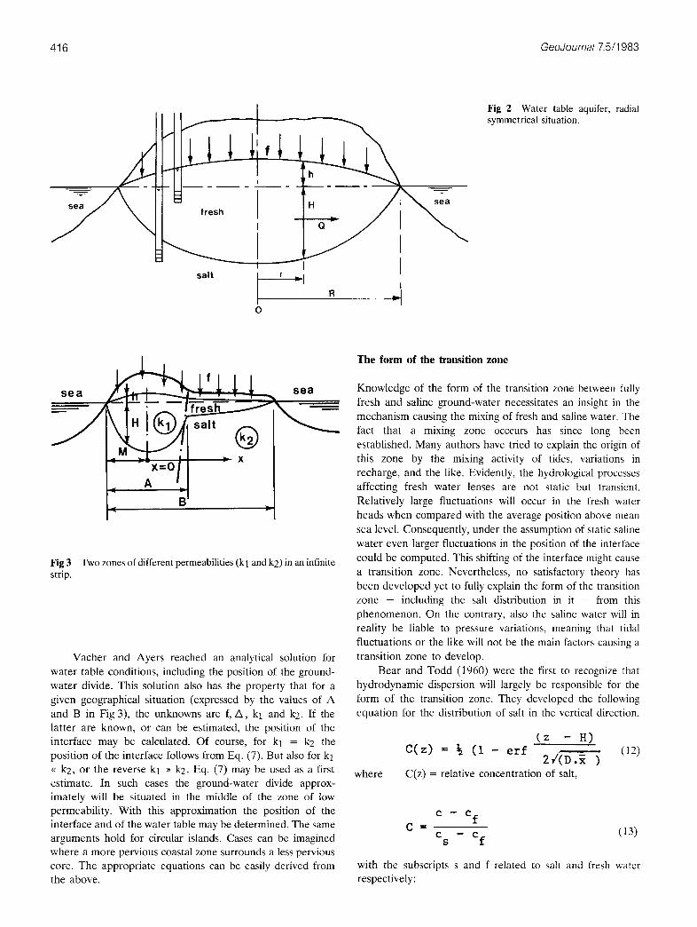
Investigations in the Guelders Valley (Meinardi 1975)

Almost everywhere in the Netherlands the occurrence of brackish ground-water has been observed. Shallow brackish ground-water is present in the areas of Holocene marine transgressions, but in the rest of the country, where the brackish water is at greater depths, the origin of the salt has to be sought in older marine sediments. Almost the whole Netherlands are underlain by marine Tertiary sediments. However, the top of the brackish ground-water bodies does not coincide with the top of the marine sediments; sometimes it is higher and sometimes lower. On the other hand, the undulations of the top of the brackish ground-water correspond with ground-water recharge and discharge areas, such that this top is lying deeper in recharge areas and is elevated below discharge areas. Furthermore, the chloride contents generally increase gradually with depth.

In view of the above situation, Meinardi (1975) conceived the idea that the salt distribution in the inland areas might largely be explained by lateral dispersion caused by a mainly horizontal ground-water flow in the aquifer system above the marine base. To verify this hypothesis, he applied Eq. (18) to regional ground-water flow (horizontal dimensions in kilometres and depth in hundreds of metres). For the investigation in the Guelders Valley (Fig 9), the following schematization and assumptions were used: - Conform to hydrogeology, the subsurface is schematized

into two layers: a shallow aquifer system where ground- water flow occurs and an impervious base. The boundary, at a depth of 350 m below msl, determines the value Z = 0 in Eq. (18).

- Instead of the dispersion coefficients A and ~, a size d (m) of the inhomogeneities in the underground has been taken into account, such that & + 2 g = d and in 3, = 0.125 d. The value of d is not know beforehand, it has to be found by trial and error, or by optimization techniques.

- As a first estimate of the basic chloride content in the stagnant salt water the value of c s = 15 000 mg C1-/1 has been chosen.

From Fig 9 we can deduce some qualitative proof that chloride distribution results from hydrodynamical dispersion: 1. The highest levels of the interface follow very closely the

ground-water divide between ground-water flow from the Veluwe and from the Utrecht Hills.

2. The tops of the interface are on the same level all along this divide, corresponding to equal length of flow lines arriving from the Veluwe.

3. The interface shows a steep slope at the side of the Utrecht Hills and a less steep one at the other side. By far the shortest flow lines originate in the Utrecht Hills.

4 2 2 GeoJoumal 7 . 5 / 1 9 8 3

!::-'.'.'. ":':'4 .-.':-:':~!:':'" :" ~ I " " , - V / r ' / . :.:-:.:.: . . . . >..:-:.:.:.: . . . . . . . . '.f-~/~,.,,~'/Z

~ i ~ / , - / , ~ . . : . : . : . : . : . ' . ....... • • , ,

A I / l l l r l - / / / / A HILLS • UTRECHT %

. . . . . . . . ,o

I ~ ~ \ " ' , , i . ~ C

a b

i 2oJ 5- ,i

3eo_electvlcal sur~ Gr~J~water surve IN.O) =ontours of CI~-IN3~p N.A.P_ m} N.A.p=Refer~nce level= mean sea I~Vel

' ~ . \ .

d

F i g 9 Data from the Guelders Valley.

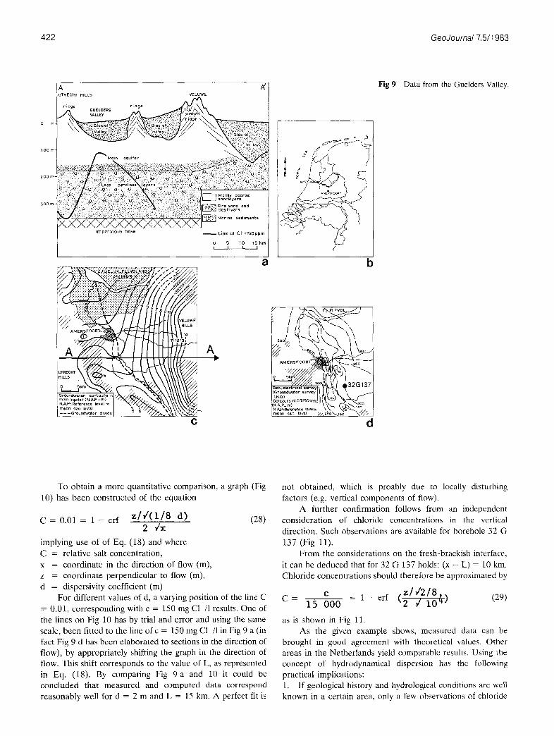
To obtain a more quantitative comparison, a graph (Fig 10) has been constructed of the equation

C = 0.01 = 1 - erf z / ¢ ' ( 1 / 8 d ) (28) 2 ,/x

implying use of of Eq. (18) and where C = relative salt concentration, x = coordinate in the direction of flow (m), z = coordinate perpendicular to flow (m), d = dispersivity coefficient (m)

For different values of d, a varying position of the line C = 0.01, corresponding with c = 150 mg CI /1 results. One of the lines on Fig l0 has by trial and error and using the same scale, been fitted to the line of c = 150 mg C1 /1 in Fig 9 a (in fact Fig 9 d has been elaborated to sections in the direction of flow), by appropriately shifting the graph in the direction of flow. This shift corresponds to the value of L, as represented in Eq. (18). By comparing Fig 9 a and 10 it could be concluded that measured and computed data correspond reasonably well for d = 2 m and L = 15 km. A perfect fit is

not obtained, which is proably due to locally disturbing factors (e.g. vertical components of flow).

A further confirmation follows from an independent consideration of chloride concentrations in the vertical direction. Such observations are available for borehole 32 G

137 (Fig 11). From the considerations on the fresh-brackish interface,

it can be deduced that for 32 G 137 holds: (x - L) = 10 km. Chloride concentrations should therefore be approximated by

- i- err ( z/~/2/8~ c

C (29) 15 000 2 ~/ i0 ~"

as is shown in Fig 11. As the given example shows, measured data can be

brought in good agreement with theoretical values. Other areas in the Netherlands yield comparable results. Using the concept of hydrodynamical dispersion has the following practical implications: 1. If geological history and hydrological conditions are well known in a certain area, only a few observations of chloride

GeoJournal 7 . 5 / 1 9 8 3 4 2 3

Fig 10 Possible positions of the line representing c = 150 mg CI-/1 in sections of the Guelders Valley along the flow direction (elaboration of Eq. (28) for variable d).

400

30_~0 50

100

- - E 5-

~ ~ ~ 100 250 ;

0 01 1 er f 300

0 350

J35000 [30000 [25000 [20000 [15000 [10000 [5000 JO ~ y , (nl) distance in the direction of flow

concentrations are needed to construct the complete picture of chloride distribution in the underground of that area. 2. Reversely, as hydrodynamic dispersion is strongly connected with ground-water flow, knowledge of chloride distribution (e.g. the fresh-brackish interface) gives an indication of the hydrological system. 3. A relatively simple hydrological investigation will already give a qualitative indication of the distribution of brackish ground-water in a certain area. 4. If dissolved constituents of ground-water other than chloride are also liable to the same physical factors, an indication on the parameters involved can be deduced from the behavior of the chloride ions. In the present investigation the transversal coefficient of hydrodynamical dispersion at horizontal flow has been determined.

Oceanic islands

Small oceanic islands often represent a situation where the B G H assumption are best met.

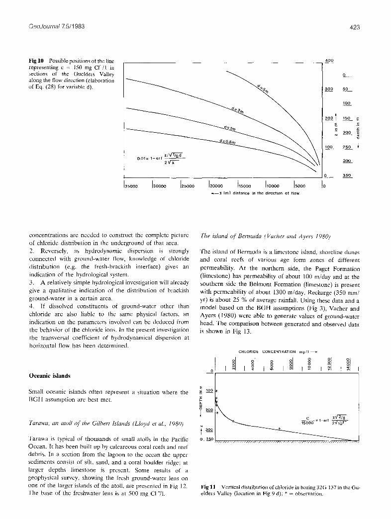
Tarawa, an atoll of the Gilbert Islands (Lloyd et al., 1980)

Tarawa is typical of thousands of small atolls in the Pacific Ocean. It has been built up by calcareous coral reefs and reef debris. In a section from the lagoon to the ocean the upper sediments consist of silt, sand, and a coral boulder ridge; at larger depths limestone is present. Some results of a geophysical survey, showing the fresh ground-water lens on one of the larger islands of the atoll, are presented in Fig 12. The base of the freshwater lens is at 500 mg CI -/1.

The island of Bermuda ( Vacher and Ayers 1980)

The island of Bermuda is a limestone island, shoreline dunes and coral reefs of various age form zones of different

permeability. At the northern side, the Paget Formation (limestone) has permeability of about 100 m/day and at the southern side the Belmont Formation (limestone) is present with permeabili ty of about 1300 m/day. Recharge (350 ram/ yr) is about 25 % of average rainfall. Using these data and a model based on the BGH assumptions (Fig 3), Vacher and Ayers (1980) were able to generate values of ground-water head. The comparison between generated and observed data is shown in Fig 13.

0

E z lO_2O

ua

N , 3oo

0 350

CHLORIDE CONCENTRATION mg/I o o o o o o

I I I I I

c z ~ 15000 = 1-erf

Fig 11 Vertical distribution of chloride in boring 32G 137 in the Gu- elders Valley (location in Fig 9 d); * = observation.

424 GeoJournat 7.5/1983

Geographical Location of Tarawa

o Guam

Papua New Guinea

"~ *~ Solomon Islands

o N e w Hebrides

5

TARAWA o !E~uator

V~ ester n %

I

X . . . . . . / 0 100 200 I t ion

T

- . -15 . . . . . depth of lens b a s e b e l o w s e a level (m)

• location ol r e s i s t i v i t y s o u d i n g s

Fig 12 Fresh ground-water lens under the Tarawa Atoll (after Lloyd et al., 1980).

1 0 elevation m

w a t e r table tao~e ....~-N

sand and silt ~ 16

-20 ~ w a b 58 64 57

l imestone

-30 base of fresh water lens

10

-40 - - 0 100 200m i i I

57 resistivity (ohm m)

SOMERSET g-Mpoe, mbrowkgs ' LENS-, / " [ --j" o, ! 2 ,

P~gg,~gg' Prospect

[Model-Observedl LP

• _< . . . . . . ~ & A . _ _ ~. & 0.05 to 009 [] ~ OAO 100.19 .. i!0.'

9 ID • > 020 " " : :

1~, [] l~ Model < Observed ~, [] () Model > Observed , : :

R=55 cm/yr R=35 cm/Y r

F i g 13 Results of a model study of Bermuda by Vacher and Ayers (1980).

S y m b o l s a n d A b r e v a t i o n s

C C

cf cp CS

D D*

d

err

erfc

exp

f

H

Hcr h

k

L

msl

mg/1

P ppm

0 q

R

r

S

t

V

V

X

R

Z

a (alpha)

- relative salt concentration A (delta)

- chloride (salt) concentration of ground-water 6 (delta) - chloride (salt) concentrat ion of fresh water k ( lambda)

- chloride (salt) concentration of pumped water ~ (mu) - chloride (salt) concentration of salt water P (rho) - dispersivity coefficient pf

- diffusion coefficient ps

- size of underground inhomogeneities

- the error function

- the complementary error function

- the exponential function

- ground-water recharge

- depth of the interface

- critical rise of the interface

- fresh ground-water head

- permeabil i ty

- length, distance

- mean sea level

- milligrams per litre (roughly equivalent to

ppm)

- porosity

- parts per million (roughly equivalent to mg/1)

- discharge, ground-water flow

- specific discharge

- radius

- polar coordinate

- second

- t ime

- dimensionless velocity

- actual velocity

- dimensionless coordinate in the direction of

flow

- coordinate in the direction of flow; horizontal

coordinate

- equivalent distance in the direction of flow

- dimensionless coordinate perpendicular to flow

- coordinate perpendicular to flow, vertical

coordinate, depth

- ion tranfer coefficient over the interface

- relative density

- percentage of pumped salt water - coefficient of the dispersion tensor - coefficient of the dispersion tensor

- density of water: - density of fresh water

- density of salt water

GeoJoumal 7.5/1983 425

References

Bear, J.: Dynamics of Fluids in Porous Media. American Elsevier, New York 1972.

Bear, J., Dagan, G.: Some Exact Solution of Interface Problems by Means of the Hodograph Method. Jour. of Geophysical Research 69, 1563- 1572 (1964)

Bear, J., Todd, D.K.: The transition zone between fresh and salt water. Water Resour. Centre Contr. 29, Berkeley, California (1960)

Dam, J.C. van: Fresh water - salt water relationships. Delft Univ. of Technology Rep. 7211, 1972.

Fetter, C.W.: Position of the Saline Interface beneath Oceanic Islands. Water Resour. Res. 8, 1307-1315, (1972)

Hunt, B.: An analysis of the ground-water resources of Tongatapu Islands, Kingdom of Tonga, Jour. of Hydrology 40, 185-196 (1979)

Lloyd, J.W. et al: A ground Water Resources Study of a Pacific Ocean Atoll - Tarawa, Gilbert Islands, Water Resour., Bull. 16, 646 -653 (1980)

Meinardi, C.R.: Brackish ground-water bodies as a result of geological history and hydrological conditions. Proc. Symposium

on Brackish Water as a Factor in Development, p. 25-39 , Beer Sheva, Israel, 1975.

Santing, G., Todd, D.K.: The development of ground-water resources with special reference to deltaic areas. UNESCO Water resources Series 24, New York, 1963.

Schmorak S., Mercado, A.: Upconing of Fresh Water - Sea Water Interface Below Pumping Wells, Field Study. Water Resour. Res. 5, 1290-1311 (1969)

Todd., D.K., Meyer, C.F.: Hydrology and geology of the Honolulu aquifer. Proc. ASCE Jour. of the Hydraulics Division, Hy 2, 2 3 3 - 2 5 6 (1971)

Vacher, H.L., Ayers, J.F.: Hydrology of small oceanic islands - utility of an estimate of recharge, inferred from the chloride concentration of the fresh water lenses. Jour. of Hydrology 45, 2 1 - 3 7 (1980)

Verruijt, A.: Steady dispension across an interface in a porous medium. Jour. of Hydrology 14, 337-347 (1971)

Volker, A.: Source of brackish groundwater in Pleistocene formations beneath the Dutch polderland. Economic Geology 56, 1045-1061 (1961)