Embed Size (px)
Citation preview

Frequency Domain Inference forSeasonally Persistent Processes
David A. Stephens
Department of Mathematics
Imperial College London
5th January, 2006
Joint work with Sofia Olhede and Emma McCoyDepartment of Mathematics, Imperial College London.
Seasonally Persistent Processes – p.1

Outline
Motivation and Notation
ARMA models
Frequency Domain Inference and The Whittle Likelihood
Persistence
Gegenbauer models
A Whittle likelihood for Seasonal Processes
Some results
Some examples
Seasonally Persistent Processes – p.2
Some real data examples
Farallon data
Carinae data
SOI data
CO2 data
Quebec Births Data
Seasonally Persistent Processes – p.3

Example : Farallon data
732 obs. monthly mean temperature at Farallon Islands, Ca,1920-1981
0 200 400 600
1011
1213
1415
16
Months (since 1920)
Mon
thly
mea
n te
mp
(C)
Figure 1:
Seasonally Persistent Processes – p.4

Example : Carinae data
1182 consecutive 10-day mean light intensities of the S.Carinæ variable star.
0 200 400 600 800 1000 1200
67
89
10
Index
Ave
rage
Inte
nsity
Figure 2:
Seasonally Persistent Processes – p.5

Example : SOI data
1688 monthly values of SOI (normalized pressure differenceTahiti/Darwin: www.cru.uea.ac.uk)
0 500 1000 1500
−4−2
02
4
Months (since 1866)
SO
I
Figure 3:
Seasonally Persistent Processes – p.6

Example : Quebec Births data
Daily number of births, in Quebec, January 1, 1977 toDecember 31, 1990.
0 1000 2000 3000 4000 5000
150
200
250
300
350
Days (since 1/1/77)
Num
ber o
f Birt
hs
Figure 4:
Seasonally Persistent Processes – p.7

Example : Quebec Births data
Weekly aggregates (from R.J. Hyndman’s Time Series DataLibrary, http://www-personal.buseco.monash.edu.au/)
0 200 400 600
1400
1600
1800
2000
2200
Months (since 1/77)
Wee
kly
Num
ber o
f Birt
hs
Figure 5:
Seasonally Persistent Processes – p.8

Example : CO2 data
468 monthly observations atmospheric concentrations of CO2
from 1959 to 1997 (from R)
Months (since 1959)
Con
cent
ratio
n (p
pm)
1960 1970 1980 1990
320
330
340
350
360
Figure 6:
Seasonally Persistent Processes – p.9

Example : CO2 data
First differences (not the only transformation possible ... )
Months (since 1959)
1st D
iffer
ence
(ppm
)
1960 1970 1980 1990
−2−1
01
2
Figure 7:Seasonally Persistent Processes – p.10

Modelling Context
Discrete time process {Xt}, zero mean
Time series data {xt : t = 1, . . . , N}Parametric models, Gaussian residual errors
Stationarity (after pre-processing)
require
likelihood-based inference about system parameters,
prediction/forecasting.
Need
likelihood,
inference mechanism.
Seasonally Persistent Processes – p.11

Time Domain modelling
Most commonly, but not exclusively, data collected in the timedomain
finance, banking, econometrics
climatology
earth sciences
computing systems, internet traffic, pageview statisticsetc.
Natural to seek inferences and make predictions in the timedomain.
Seasonally Persistent Processes – p.12

Autocovariance
In the time domain, raw data plots are not that informative;the stationary process is characterized by its autocovariancesequence (acvs)
γk = E[XtXt+k] k ∈ Z
Determination of underlying structure is more straightforwardafter inspection of the acvs/autocorrelation sequence.
Seasonally Persistent Processes – p.13

ACF plot comparison
0 10 20 30 40 50
−0.
20.
00.
20.
40.
60.
81.
0
Lag
AC
F
Farallon data
0 10 20 30 40 50
0.0
0.2
0.4
0.6
0.8
1.0
Lag
AC
F
SOI data
Seasonally Persistent Processes – p.14

Starting Point: ARIMA Models
{Xt} with zero mean follows an ARIMA(p, d, q) model if
Φ(B)∆dXt = Θ(B)ǫt,
B is the backward shift operator, so that BXt = Xt−1.
∆d = (1 −B)d, where d is the positive, integer-valuedlevel of differencing required to achieve stationarity.
{ǫt} is a zero mean Gaussian error process with varianceσ2
ǫ .
yields a Gaussian likelihood in the time domain.
Seasonally Persistent Processes – p.15

The process is specified by the AR and MA polynomials
Φ(B) = 1 − φ1B − ...− φpBp Θ(B) = 1 + θ1B + ...+ θqB
q
with real-valued parameters φj 6= 0, θj 6= 0.
Sufficient conditions for stationarity and invertibility of thedifferenced series Yt = ∆dXt are that the roots of the twopolynomial equations
Φ(z) = 0 Θ(z) = 0
lie outside the unit circle. Under these conditions, ARMAprocesses have infinite AR and MA representations.
Seasonally Persistent Processes – p.16

Parameterization
Under the restrictions of stationarity/invertibility, theparameter space for general (p, q) is a region in R
p+q that isnot straightforward.
This makes inference (e.g. MCMC) difficult to implement.
Can use a reciprocal root parameterization (Huerta and West(1999)): write
Φ(z) =
p∏
j=1
(1 − ζ1jz) Θ(z) =
q∏
j=1
(1 − ζ2jz),
where (ζ11, ..., ζ1p) and (ζ21, ..., ζ2q) are complex-valuedparameters.
Seasonally Persistent Processes – p.17

For both Φ and Θ, the reciprocal roots are either real, orappear in complex conjugate pairs. Denote by
(p1, p2), and (q1, q2) the number of real and complexconjugate pairs (so that p = p1 + 2p2, q = q1 + 2q2).
For the complex roots, for r = 1, 2
ζrj = αrjei2πωrj = αrj cos 2πωrj + iαrj sin 2πωrj ;
ζrj+1 = αrje−i2πωrj = αrj cos 2πωrj − iαrj sin 2πωrj.
For stationarity/invertibility:
0 ≤ α1j, α2j < 1 0 ≤ ω1j, ω2j < 1/2.
Seasonally Persistent Processes – p.18

MCMC Inference in the Time Domain
Using this parameterization, it is possible to implement(transdimensional) MCMC in a reasonably straightforwardfashion.
Model space defined by p, q,
Birth/Death moves to change dimension,
Metropolis-Hastings moves on θ and φ,
Can incorporate different degrees of differencing.
However computation of Gaussian likelihood requiresinversion of potentially large covariance matrix. This canbe prohibitive.
Seasonally Persistent Processes – p.19

Frequency Domain RepresentationSpectral representation of the acvs of {Xt}:
γk =
∫ 1/2
−1/2
exp {2πikf} dSI(f) =
∫ 1/2
−1/2
exp {2πifk}S(f)df.
SI(f) is a non-decreasing function on (−1/2, 1/2),
derivative S(f), the Spectral Density Function (SDF)
S(f) gives a decomposition of the variance of the processinto contributions of different frequencies.
S(f) =∞∑
k=−∞
γk exp {−2πifk} .
Seasonally Persistent Processes – p.20

SDF for ARMA processes
The stationary ARMA(p, q) process {Xt} has SDF
S(f) = σ2ǫ
|Θ(ei2πf )|2|Φ(ei2πf )|2 = σ2
ǫ
q∏
j=1
∣
∣1 − ζ2jei2πf∣
∣
2
p∏
j=1
|1 − ζ1jei2πf |2.
This function is
bounded
bounded away from zero.
Seasonally Persistent Processes – p.21

The Periodogram
At the Fourier frequencies, fj = j/N , j = 0, . . . , N/2, defineperiodogram, I, by
I(fj) = |Z(fj)|2 j = 0, . . . , N/2
where Z is the Discrete Fourier Transform (DFT) of {Xt}
Z(fj) =1√N
N−1∑
t=0
Xte−i2πtfj = Aj + iBj
I(fj) =1
N
[
N−1∑
t=0
X2t + 2
N−1∑
t=1
t−1∑
s=0
XtXs cos (2πj(t− s)/N)
]
Seasonally Persistent Processes – p.22

The periodogram is a natural non-parametric estimator for S
I(fj) and I(fk), j 6= k are asymptotically independent
I asymptotically unbiased for S (in most cases)
inconsistent
always finite valued.
Behaviour as N → ∞ illustrates problem; the grid of Fourierfrequencies has O(N) components, so the learning rate iszero (we essentially have just a data transformation).
Seasonally Persistent Processes – p.23
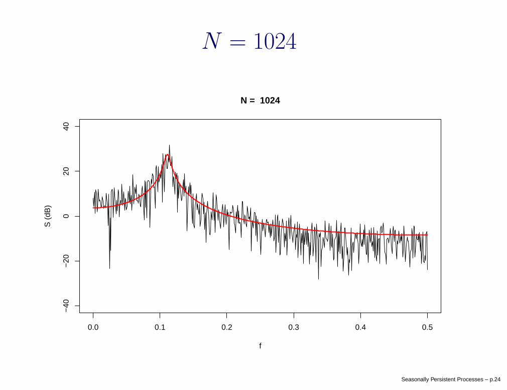
N = 1024
0.0 0.1 0.2 0.3 0.4 0.5
−40
−20
020
40
f
S (
dB)
N = 1024
Seasonally Persistent Processes – p.24

0.0 0.1 0.2 0.3 0.4 0.5
−40
−20
020
40
f
S (
dB)
N = 2048
0.0 0.1 0.2 0.3 0.4 0.5
−40
−20
020
40
f
S (
dB)
N = 4096
0.0 0.1 0.2 0.3 0.4 0.5
−40
−20
020
40
f
S (
dB)
N = 8192
0.0 0.1 0.2 0.3 0.4 0.5
−40
−20
020
40
f
S (
dB)
N = 16384
Seasonally Persistent Processes – p.25

Examples Revisited
0.0 0.1 0.2 0.3 0.4 0.5
−30
−20
−10
010
20
Frequency
Per
iodo
gram
(dB
)
Farallon
0.0 0.1 0.2 0.3 0.4 0.5
−20
−10
010
Frequency
Per
iodo
gram
(dB
)
SOI
Seasonally Persistent Processes – p.26
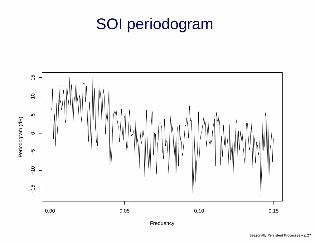
SOI periodogram
0.00 0.05 0.10 0.15
−15
−10
−5
05
1015
Frequency
Per
iodo
gram
(dB
)
Seasonally Persistent Processes – p.27

Likelihood Inference
See Chan and Palma (2004) for a recent summary:
exact time domain
approximate time domain
AR approximation
MA approximation
QML
exact frequency domain
approximate frequency domain
Most exact methods are at least O(N 2) per likelihoodevaluation in computation.
Seasonally Persistent Processes – p.28

The Whittle Likelihood
Motivation: Approximate the Gaussian time-domain likelihoodusing a spectral approximation to covariance matrix Σ
(Whittle (1951, 1953), Grenander and Szëgo (1958))
1
NlogL(θ, φ) = − 1
2Nlog |Σ(θ, φ)| − 1
2NXT Σ(θ, φ)−1X
≈ − 1
2N
{
N∑
j=1
log S(ωj; θ, φ) +
N∑
j=1
I(ωj)
S(ωj; θ, φ)
}
where ωj = 2πfj = 2πj/N .
Seasonally Persistent Processes – p.29

Statistical Properties
For models with bounded spectra, for N large,
I(fj)/S(j/N)L= Uj, j = 0, . . . ,M = N/2
Uj ∼ χ22/2 ≡ Exp(1) i.i.d., j = 1, . . . ,M − 1,
U0, UM ∼ χ21
These properties facilitate likelihood-based inference via theWhittle approximation.
ML estimates of SDF parameters are consistent andasymptotically normally distributed.
Seasonally Persistent Processes – p.30

Seasonally Persistent ProcessesIt is plausible in many contexts that {Xt} has a seasonalcomponent
calendar-based data collection (annual, quarterly,monthly, or weekly cycles)
high dependence at specific lags
using seasonal differencing e.g. for monthly data
Yt = (1 −B12)Xt = Xt −Xt−12
removes an annual seasonal component.
Seasonal processes are not stationary before differencing,and have SDFs with singularities (poles) that render the SDFnot integrable.
Seasonally Persistent Processes – p.31

Persistence : A process {Xt} with acvs {γk} can also exhibitpersistence, that is,
long-range dependence if, ∀a > 0
limk→∞
a−k
γk
= 0
that is, the acf is slowly decaying.
long-memory if the acvs is absolutely divergent∑
k
|γk| = ∞
in practice, diagnosed by observing large autocorrelationat high lags, spectral power near frequency zero.
Seasonally Persistent Processes – p.32

Constructing Persistent ProcessesLet {Wt} be an i.i.d. Gaussian sequence with variance 1. Letδ ∈ (−1/2, 1/2), and write
(1 − B)δ =∞∑
k=0
ck(−δ)(−B)k ck(d) =Γ(k + d)
Γ(k + 1)Γ(d)
and set Xt = (1 −B)−δWt.
This fractional differencing yields a process that is stationaryif δ < 1/2, long-memory if 0 < δ < 1/2 and long-rangedependent if −1/2 < δ < 1/2. For k large,
γk ∼ k−(1−2δ)
The persistence is associated with frequency zero.Seasonally Persistent Processes – p.33

Periodograms for different δ.
0.0 0.1 0.2 0.3 0.4 0.5
01
02
03
04
05
06
0
f
10
log
10(I)
d = 0.1
0.0 0.1 0.2 0.3 0.4 0.5
01
02
03
04
05
06
0
f
10
log
10( I)
d = 0.2
0.0 0.1 0.2 0.3 0.4 0.5
01
02
03
04
05
06
0
f
10
log
10(I)
d = 0.3
0.0 0.1 0.2 0.3 0.4 0.5
01
02
03
04
05
06
0
f
10
log
10( I)
d = 0.4
Seasonally Persistent Processes – p.34

Seasonal Persistence
Similar construction: replace {ck} sequence by {gk} suchthat, for some λ0 ∈ (0, 1/2),
Xt = (1 − 2 cos(2πλ0)B +B2)−δWt
Recursion for {gk} given by g−1 = 0, g0 = 1 and for k > 0
gk =
(
2
k + 1
)
(δ + k) cos(2πλ0) −(
2δ + k − 1
k + 1
)
gk−1
but no simple explicit form.
{gk} are coefficients of the Gegenbauer polynomials (seeGray, Zhang, Woodward (1989), Lapsa(1997)).
Seasonally Persistent Processes – p.35

This procedure yields a process {Xt} that has persistenceassociated with the frequency λ0, and is stationary
if δ < 1/2 when λ0 6= 0, or
if δ < 1/4 when λ0 = 0
SDF has relatively straightforward form
S(f) =1
(2 |cos(2πf) − cos(2πλ0)|)2δ
with
S(f) → 1
(2 |sin(2πλ0)|)2δ
1
|2πf − 2πλ0|2δf → λ0
Seasonally Persistent Processes – p.36

ACV/ACF less straightforward
σ2Xγk =
Γ(1 − 2δ)√π21/2+2δ
{sin(2πλ0)}1/2−2δ
[
P2δ−1/2k−1/2 (cos(2πλ0)) + (−1)kP
2δ−1/2k−1/2 (− cos(2πλ0))
]
where P µν (x) is the associated Legendre function of the first
kind.
A recursion formula for P µν (x) gives the acvs to arbitrary lag.
(ν − µ+ 1)P µν+1(x) = (2ν + 1)P µ
ν (x) − (ν + µ)P µν−1(x)
Seasonally Persistent Processes – p.37

Gegenbauer Models
Characteristic singularity (pole) in the spectrum at λ0.
0.0 0.1 0.2 0.3 0.4 0.5
−5
05
1015
2025
f
S(f
) (d
B)
0.10.20.30.4
λ0 =0.14
Seasonally Persistent Processes – p.38

Example: λ0 = 0.14, δ = 0.4
0 100 200 300 400 500
−4
−2
02
4
Time
X
Data
0 10 20 30 40 50
−0.
50.
00.
51.
0
Lag
AC
F
ACF
Seasonally Persistent Processes – p.39

Theoretical ACF
With δ = 0.4, large autocorrelation at high lag separation.
0 100 200 300 400 500
−1.
0−
0.5
0.0
0.5
1.0
Lag
AC
F
Seasonally Persistent Processes – p.40

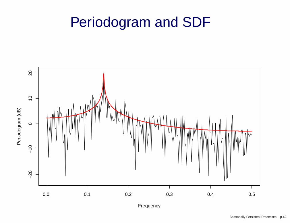
Periodogram
0.0 0.1 0.2 0.3 0.4 0.5
−20
−10
010
20
Frequency
Per
iodo
gram
(dB
)
Seasonally Persistent Processes – p.41
Periodogram and SDF
0.0 0.1 0.2 0.3 0.4 0.5
−20
−10
010
20
Frequency
Per
iodo
gram
(dB
)
Seasonally Persistent Processes – p.42

The Whittle Likelihood for SP process
The distributional assumptions central to the construction ofthe Whittle likelihood break down for Fourier frequenciesnear to spectral poles.
Recall that the periodogram is finite at the pole λ0, where theSDF is not finite.
When the pole is at λ0 = 0 (standard long-memory), it ispossible to deduce distributional properties for theperiodogram evaluated at the Fourier frequencies.
Seasonally Persistent Processes – p.43

For example, Hurvich and Beltrao (1993): when the pole is atλ0 = 0.
the periodogram values should not treated as i.i.dexponential random variables
asymptotically, the periodogram values are distributed aweighted combination of two independent χ2
1 randomvariables.
the asymptotic relative bias in the periodogram is positivefor most values of the δ parameter.
We attempt to re-evaluate these results for general λ0.
Seasonally Persistent Processes – p.44

Relabelling the Fourier frequencies
We attempt to quantify the (relative) bias in the periodogramat Fourier frequencies near to λ0.
The bias will depend on the distance between the Fourierfrequency and λ0.
For any fixed λ0, the distance from the pole to the nearestFourier frequency depends on sample size N .
Intuitively, as the distance decreases, the bias increases.
For convenience, we re-label the Fourier frequencies, so thatf ′
j is the j th closest Frequency to the pole.
Seasonally Persistent Processes – p.45

The grid of Fourier frequencies m/N for integer m, and theirrelation to the Fourier frequencies closest to the pole. Hereω1/(2π) = m/N and ω2/(2π) = (m− 1)/N .
00
λ0 m/N(m−1)/N(m−2)/N
|c1,N
(λ0)|/N|c
2,N(λ
0)|/N
λSeasonally Persistent Processes – p.46

Quantifying the relative bias
The crucial factor determining the magnitude of the bias is thedistance between the periodogram ordinates and λ0.
THEOREM : For (relabelled) Fourier frequency f ′j, the j th
closest to the pole at λ0, for large N
E
(
I(
f ′j
)
S(
f ′j
)
)
=2
π
∫ ∞
−∞
sin2 {u/2 − πcj,N (λ0)}{u− 2πcj,N (λ0)}2
∣
∣
∣
∣
2πcj,N(λ0)
u
∣
∣
∣
∣
2δ
du
plus terms that are o(1), where cj,N(λ0) = j −Nλ0.
Seasonally Persistent Processes – p.47

Bias for various values of (c, δ)
The bias varies from minimal to considerable.
0.10.2
0.30.4
0.51
1.52
2.53
0
2
4
6
8
10
δ
Expected Value of Normalized Periodogram
c
Figure 7:
Seasonally Persistent Processes – p.48

Demodulation
The Demodulated DFT (DDFT) or offset DFT (Pei and Ding(2004)) of Xt, with demodulation via frequency λ is denotedZλ, and is defined for fj = j/N by
Zλ (fj) =1√N
N−1∑
t=0
Xte−2iπ(fj+λ)t = Aλ,j + iBλ,j, j = 0, . . . ,M.
The demodulated periodogram at frequency fj withdemodulation via λ is denoted Iλ(fj), and is defined via theordinary periodogram I by
Iλ(fj) = I(fj + λ) = |Zλ(fj)|2 = A2λ,j(j) +B2
λ,j.
Seasonally Persistent Processes – p.49

Demodulation simplifies the calculation of distributionalproperties of periodogram values near the spectral pole.
THEOREM : For a Gegenbauer (λ0, δ) process with SDF
S (f) = S†(f) |f − λ0|−2δ
where S† is a bounded SDF, the expected value of theperiodogram evaluated at the pole λ0, after demodulation byλ0, is
(2πN)2δ{−2S†(λ0)Γ(−1 − 2δ)} cos{π(1/2 + δ)}π−1 + o(1)
which is O(N 2δ).
Seasonally Persistent Processes – p.50

A Whittle Likelihood Adjustment
Using the previous theorem, and demodulation, we canconstruct an adjusted Whittle likelihood to estimate theparameters in the SPP.
For a Gegenbauer model with parameters (λ0, δ), construct ademodulated Whittle likelihood as follows:
Compute the DDFT of sample data with demodulation viaλD = λ0 − [Nλ0]/N ; this aligns a new Fourier gridprecisely with λ0.
Seasonally Persistent Processes – p.51

This yields periodogram values
I(λ0 + J1/N), . . . I(λ0 + J2/N)
where J1 = −[Nλ0] and J2 = (N/2) − [Nλ0].
Construct a likelihood under the model where
I(λ0 + j/N) ∼ Exp(ηj)
give independent contributions, and
ηj =|j|2δχ{j 6=0}
Q(δ)χ{j=0}N 2δS†(λ0 + j/N)
where Q(δ) = −Γ (−1 − 2δ) cos{π (1/2 + δ)}22δ+1π2δ−1.
Seasonally Persistent Processes – p.52

This likelihood is bounded on (0, 1/2) × (0, 1/2).
It is not continuous in λ0 due to the demodulation, but thediscontinuities are O(1), hence ignorable.
Numerical maximization yields ML estimates.
Theoretical properties of the estimators are notstraightforward to establish.
In particular, the behaviour of the the estimator of λ0 isnon-standard.
Seasonally Persistent Processes – p.53

Asymptotic Properties of the Estimators
For the adjusted likelihood, we can establish
N -consistency for λ̂0, N 1/2-consistency for δ̂
asymptotic normality of δ̂
asymptotic distribution of λ̂0 is scaled Cauchy
Simulation studies verify that demodulated likelihood yieldsestimators that seem to have better small sampleperformance than the classic Whittle likelihood when λ0 isunknown.
Seasonally Persistent Processes – p.54

Sampling distribution of estimator
Simulation study: 1000 reps., N = 4096, λ0 = 1/7, δ = 0.4λ0
λ0
Fre
quen
cy
0.1420 0.1425 0.1430 0.1435
010
020
030
040
050
0
δ
δ
Fre
quen
cy
0.36 0.38 0.40 0.42 0.44
050
100
150
Seasonally Persistent Processes – p.55

Small sample properties
A simulation study: λ0 = 0.15, δ = 0.1, 0.2, 0.3, 0.4, N = 406,1000 replicate data sets.
Adjusted Whittle Classic Whittle
δ Mean SD Mean SD
0.1 0.104 0.0294 0.100 0.0283
0.2 0.199 0.0312 0.194 0.0316
0.3 0.298 0.0313 0.297 0.0325
0.4 0.399 0.0291 0.405 0.0330
Seasonally Persistent Processes – p.56
Non likelihood estimation
Geweke-Porter-Hudak (GPH); semi-parametric,generalized least-squares using periodogram nearsingularity.
Giraitis-Hidalgo-Robinson; minimize the discrepancymeasure
G (δ, λ0) =1
M
M∑
j=0
I(j/N)
SGHR (j/N ;λ0, δ).
over a “fine grid" of values for λ0.
also common to choose λ̂0 equal to the Fourier frequencyat which the periodogram achieves its maximum value(Hidalgo-Soulier).
Seasonally Persistent Processes – p.57
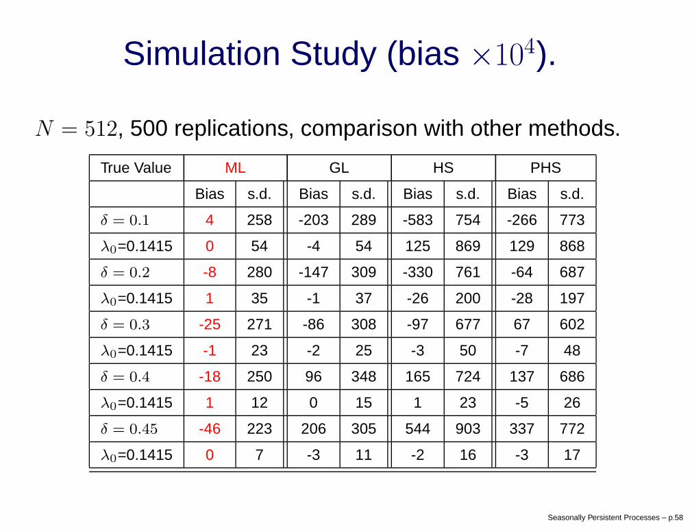
Simulation Study (bias ×104).
N = 512, 500 replications, comparison with other methods.
True Value ML GL HS PHS
Bias s.d. Bias s.d. Bias s.d. Bias s.d.
δ = 0.1 4 258 -203 289 -583 754 -266 773
λ0=0.1415 0 54 -4 54 125 869 129 868
δ = 0.2 -8 280 -147 309 -330 761 -64 687
λ0=0.1415 1 35 -1 37 -26 200 -28 197
δ = 0.3 -25 271 -86 308 -97 677 67 602
λ0=0.1415 -1 23 -2 25 -3 50 -7 48
δ = 0.4 -18 250 96 348 165 724 137 686
λ0=0.1415 1 12 0 15 1 23 -5 26
δ = 0.45 -46 223 206 305 544 903 337 772
λ0=0.1415 0 7 -3 11 -2 16 -3 17
Seasonally Persistent Processes – p.58

Examples revisited: Farallon Data
0.1 0.2 0.3 0.4
0.1
0.2
0.3
0.4
λ0
δ
Log−likelihood surface for Farallon data (Adjusted Whittle)
0.1 0.2 0.3 0.4
0.1
0.2
0.3
0.4
λ0
δ
Log−likelihood surface for Farallon data (Classic Whittle)
Figure 7:
Seasonally Persistent Processes – p.59

Posterior Distributions : λ0
Adjusted (N=444)
farbayes0.lam
Fre
quen
cy
0.075 0.080 0.085 0.090 0.095
010
020
030
040
0
Classic (N=444)
farclassic0.lam
Fre
quen
cy
0.075 0.080 0.085 0.090 0.095
050
100
150
200
250
300
Adjusted (N=440)
farbayes1.lam
Fre
quen
cy
0.075 0.080 0.085 0.090 0.095
010
020
030
0
Classic (N=440)
farclassic1.lam
Fre
quen
cy
0.075 0.080 0.085 0.090 0.095
050
100
150
Seasonally Persistent Processes – p.60
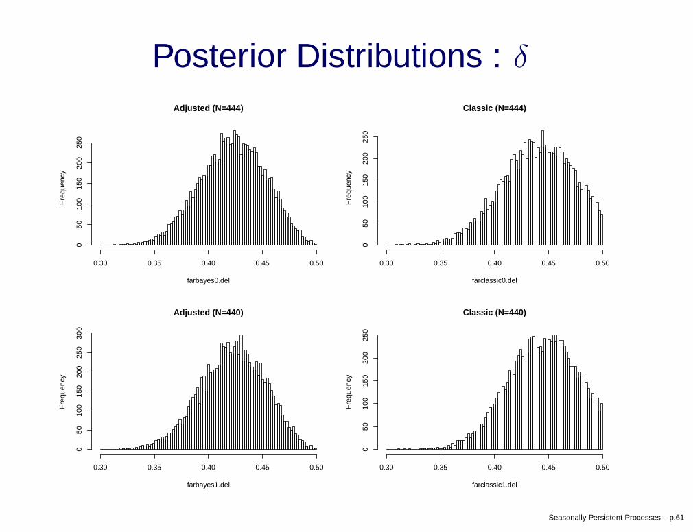
Posterior Distributions : δAdjusted (N=444)
farbayes0.del
Fre
quen
cy
0.30 0.35 0.40 0.45 0.50
050
100
150
200
250
Classic (N=444)
farclassic0.del
Fre
quen
cy
0.30 0.35 0.40 0.45 0.50
050
100
150
200
250
Adjusted (N=440)
farbayes1.del
Fre
quen
cy
0.30 0.35 0.40 0.45 0.50
050
100
150
200
250
300
Classic (N=440)
farclassic1.del
Fre
quen
cy
0.30 0.35 0.40 0.45 0.50
050
100
150
200
250
Seasonally Persistent Processes – p.61

Examples revisited: SOI data (N = 1688)
0.1 0.2 0.3 0.4
0.1
0.2
0.3
0.4
λ0
δ
Log−likelihood surface for SOI data (Adjusted Whittle)
0.1 0.2 0.3 0.4
0.1
0.2
0.3
0.4
λ0
δ
Log−likelihood surface for SOI data (Classic Whittle)
Figure 7:
Seasonally Persistent Processes – p.62

GARMA Models
The spectrum of a k-factor GARMA model;
S(f) = σ2ǫ
q∏
j=1
∣
∣
(
1 − ζ2jei2πf)∣
∣
2
p∏
j=1
|(1 − ζ1jei2πf )|21
k∏
j=1
[
4 {cos(2πf) − ψj}2]δj
,
where ψj = cos(2πλ0j) parameterizes the location of the jthsingularity in the spectrum.
Use variable dimension MCMC to carry out inference andprediction.
Seasonally Persistent Processes – p.63

Examples revisited: Carinae data
0.0 0.1 0.2 0.3 0.4 0.5
−40
−30
−20
−10
010
20
Frequency
Per
iodo
gram
(dB
)
Carinae
Figure 7:
Seasonally Persistent Processes – p.64
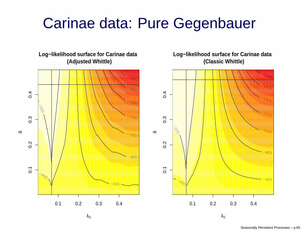
Carinae data: Pure Gegenbauer
0.1 0.2 0.3 0.4
0.1
0.2
0.3
0.4
λ0
δ
Log−likelihood surface for Carinae data (Adjusted Whittle)
0.1 0.2 0.3 0.4
0.1
0.2
0.3
0.4
λ0
δ
Log−likelihood surface for Carinae data (Classic Whittle)
Figure 7:
Seasonally Persistent Processes – p.65

GARMA fit using MCMC
••••••
•
•
•••••••
•
••
•
••
•
••••
•
••••••
•
••••••••
•••••
••••
•
•••
••
••••
•••••
•
•••••
••••
••
•
•
•
•••••
•
•••
•
•
•••••
•
••••••••••
•
••••••••
•
•
•••••
•
••••
••••
•
••••••••
•
••••
••
••
•
•••
••
••
••••
••
•
•••
•
••••••••••
•
•
•
•
•
•
••
••
•
••••••
•
•
•
•••
•••
•
••
••••
••
•
•••
•
••
•••
•
•
•••••••••••
••
•
••••••
•
••••••
•••
••
•
•
•••
••
••
•
•
••
•
•••••••••••
•
•
••
••••
•
•
•
•••••••••
••••••••••••••••
••
•
•••
•
••••
••••••••
•
•••
•
•
••••
••
•
•
•
••
•
••
••
•
•
••
•
••••
••••
•
••••••
•
••
••
••••••
••
•
••
•••••••
••••••
••••••••
••
••
••
•••••
•
••
•
•••
•••
•
•••••
•
••
••
•
•••••••
•••••
•
•
•
•••••••••••
•
•
•••
••••
••
•
••
•
•
•••
•
•••
•
•••
••••••••••
•
••••
•
••
•
•
•
•
•
•
•
•
•
•••
•
•••
•
•••••••••••••
•••••••
•
••
••••
•
••
•
••
•
••••••••
•••••
••••
•
frequency
dB
0.0 0.1 0.2 0.3 0.4 0.5
-60
-40
-20
0
MedianQuartiles2.5th & 97.5th Quantiles
Spectral Density: Posterior Summary
Spectral Density: Posterior Samples
Seasonally Persistent Processes – p.66

Extensions
Whittle adjustments for multiple Gegenbauer models
modelling harmonics
adjustments to current semiparametric methods
adjusted continuous Whittle likelihood
MCMC inference, model selection, imputation of missingvalues, prediction
prediction (forecasting) required in time domain
inference in frequency domain ?
achieved using data augmentation technique inMCMC.
Seasonally Persistent Processes – p.67