Frequency Domain Based Analysis and Design of Norm-Optimal

Frequency Domain Based Analysis and Design ofNorm-Optimal Iterative Learning Control

by

Xinyi Ge

A dissertation submitted in partial fulfillmentof the requirements for the degree of

Doctor of Philosophy(Mechanical Engineering)

in The University of Michigan2017

Doctoral Committee:

Professor Jeffrey L. Stein, Co-ChairDr. Tulga Ersal, Co-ChairAssociate Professor Brent GillespieProfessor Jing Sun

Xinyi Ge

[email protected]

ORCID iD: 0000-0002-4005-4252

c© Xinyi Ge 2017

All Rights Reserved

ACKNOWLEDGEMENTS

Foremost, I would like to express my sincere gratitude to my advisors, Prof. Jeffrey

L. Stein and Dr. Tulga Ersal. Without their excellent guidance, constant support

and remarkable patience, I don’t think I would ever have finished this work. I am

honored to have been their student and deeply grateful for all I have learned from

them.

Besides my advisors, I also want to convey my warm and sincere thanks to the

rest of my committee members, Prof. Brent Gillespie and Prof. Jing Sun, for their

insightful comments and valuable suggestions towards my research. I believe that

their insightful feedbacks have led this dissertation to be more thorough and complete.

I also wish to express my gratitude to my fellow lab mates in for the stimulating

discussions and for all the fun we have had along my Ph.D journey.

I also would like to thank all my friends in my life. I value their friendship very

much and it is their support all the way long that has brought where I am today.

Thank you all very much!

Finally, I must express my very profound gratitude to my parents and to my fiancee

for providing me with unfailing support and continuous encouragement throughout

my years of study and through the process of researching and writing this thesis.

This accomplishment would not have been possible without them. Thank you and I

always love you!

ii

TABLE OF CONTENTS

ACKNOWLEDGEMENTS . . . . . . . . . . . . . . . . . . . . . . . . . . ii

LIST OF FIGURES . . . . . . . . . . . . . . . . . . . . . . . . . . . . . . . v

ABSTRACT . . . . . . . . . . . . . . . . . . . . . . . . . . . . . . . . . . . ix

CHAPTER

I. Introduction . . . . . . . . . . . . . . . . . . . . . . . . . . . . . . 1

1.1 Brief Introduction to Iterative Learning Control . . . . . . . . 11.2 An Overview of ILC Literature . . . . . . . . . . . . . . . . . 21.3 Focus of This Work . . . . . . . . . . . . . . . . . . . . . . . 61.4 Thesis Contributions and Outline . . . . . . . . . . . . . . . . 11

II. Background of NO-ILC . . . . . . . . . . . . . . . . . . . . . . . 13

2.1 System Representation . . . . . . . . . . . . . . . . . . . . . . 132.2 Derivation of NO-ILC Updating Law . . . . . . . . . . . . . . 152.3 Monotonic Convergence . . . . . . . . . . . . . . . . . . . . . 152.4 Modeling Error . . . . . . . . . . . . . . . . . . . . . . . . . . 172.5 NO-ILC in Frequency Domain . . . . . . . . . . . . . . . . . 18

III. Model Uncertainty Formulation . . . . . . . . . . . . . . . . . . 19

3.1 Model Uncertainty . . . . . . . . . . . . . . . . . . . . . . . . 193.2 Frequency Domain RMC Criterion . . . . . . . . . . . . . . . 233.3 Existing Graphical Interpretation on RMC . . . . . . . . . . 273.4 Conclusion . . . . . . . . . . . . . . . . . . . . . . . . . . . . 29

IV. RMC Analysis and Design Tools . . . . . . . . . . . . . . . . . . 31

4.1 Diagonal Weighting Matrices Design . . . . . . . . . . . . . . 324.1.1 RMC of NO-ILC without Q-Filter . . . . . . . . . . 32

iii

4.1.2 RMC of NO-ILC with Q-Filter . . . . . . . . . . . . 354.1.3 Design Guideline . . . . . . . . . . . . . . . . . . . 384.1.4 Simulation Examples . . . . . . . . . . . . . . . . . 40

4.2 Frequency Dependent Weighting Matrices Design . . . . . . . 514.2.1 RMC Analysis . . . . . . . . . . . . . . . . . . . . . 524.2.2 Design Guideline . . . . . . . . . . . . . . . . . . . 544.2.3 Simulation Examples . . . . . . . . . . . . . . . . . 57

4.3 Conclusion . . . . . . . . . . . . . . . . . . . . . . . . . . . . 64

V. Fundamental Trade-off of NO-ILC and Its Optimality . . . . 65

5.1 Fundamental Trade-off Between Robustness, Convergence Speedand Steady State Error . . . . . . . . . . . . . . . . . . . . . 66

5.1.1 Robustness . . . . . . . . . . . . . . . . . . . . . . . 665.1.2 Convergence Speed . . . . . . . . . . . . . . . . . . 675.1.3 Steady State Error . . . . . . . . . . . . . . . . . . 685.1.4 Expressing the Fundamental Trade-off for NO-ILC . 695.1.5 Simulation Example . . . . . . . . . . . . . . . . . . 70

5.2 Optimality of NO-ILC . . . . . . . . . . . . . . . . . . . . . . 765.2.1 Without Q-Filter . . . . . . . . . . . . . . . . . . . 775.2.2 With Q-Filter . . . . . . . . . . . . . . . . . . . . . 81

5.3 Conclusion . . . . . . . . . . . . . . . . . . . . . . . . . . . . 84

VI. Optimization Formulation towards NO-ILC Design . . . . . . 85

6.1 Design for Optimal Nominal Performance . . . . . . . . . . . 866.1.1 Problem Setup . . . . . . . . . . . . . . . . . . . . . 866.1.2 Optimization Setup to Design the Filters . . . . . . 876.1.3 Least Squares Setup to Obtain the Weighting Matrices 89

6.2 Design for Optimal Performance Under Uncertainties . . . . . 916.2.1 Disadvantage of the Nominal Performance Based De-

sign . . . . . . . . . . . . . . . . . . . . . . . . . . . 916.2.2 Design Against Uncertainties . . . . . . . . . . . . . 92

6.3 Summary of Design Procedure . . . . . . . . . . . . . . . . . 946.4 Simulation Examples . . . . . . . . . . . . . . . . . . . . . . . 95

6.4.1 Example 1 . . . . . . . . . . . . . . . . . . . . . . . 956.4.2 Example 2 . . . . . . . . . . . . . . . . . . . . . . . 99

6.5 Conclusion . . . . . . . . . . . . . . . . . . . . . . . . . . . . 100

VII. Concluding Remarks and Future Work . . . . . . . . . . . . . . 103

APPENDICES . . . . . . . . . . . . . . . . . . . . . . . . . . . . . . . . . . 107

BIBLIOGRAPHY . . . . . . . . . . . . . . . . . . . . . . . . . . . . . . . . 116

iv

LIST OF FIGURES

Figure

1.1 Shooting athlete can improve shooting accuracy by repetitive practice 2

1.2 A standard progression in the error and control signal over severaliterations with the use of ILC . . . . . . . . . . . . . . . . . . . . . 3

2.1 Formulation of modeling error in the (a) time and (b) frequency domain 17

3.1 Example model uncertainty expressed on the Bode plot . . . . . . . 20

3.2 Model uncertainty in Fig. 3.1 expressed on the Nyquist Plot at fre-quency of (a) ω1 and (b) ω2 . . . . . . . . . . . . . . . . . . . . . . 21

3.3 Comparison of the proposed and traditional model uncertainty for-mulations . . . . . . . . . . . . . . . . . . . . . . . . . . . . . . . . 23

3.4 An illustration of ui+1 and ui+1(z) obtained through Eq. (3.3) . . . 24

3.5 Graphical interpretation of Eq. (3.9) . . . . . . . . . . . . . . . . . 28

4.1 Geometric representation of RMC region of NO-ILC without Q-filter 34

4.2 Geometric representation of RMC region of NO-ILC with Q-filter . 37

4.3 Illustration of the benefits of the proposed approach: (a) the uncer-tainty regions and (b) the RMC disks resulting from the traditionaland proposed uncertainty formulations. . . . . . . . . . . . . . . . . 39

4.4 Achieving RMC for the example model uncertainty regions at twofrequencies . . . . . . . . . . . . . . . . . . . . . . . . . . . . . . . . 40

4.5 Bode plot of G (z), Go (z), Gmax (z), Gmin (z) and uncertainty regionfor Example 1 . . . . . . . . . . . . . . . . . . . . . . . . . . . . . . 42

v

4.6 RMC disks with different λ values and uncertainty region at a fre-quency of 13.23 rad/s on the Nyquist plot for Example 1 . . . . . . 43

4.7 Tracking results of NO-ILC with λ = 9 and λ = 16 in Example 1 . . 44


4.9 RMC disks with two NO-ILC designs and uncertainty region at afrequency of 1.05 rad/s on the Nyquist plot for Example 2 . . . . . 46

4.10 Tracking results of NO-ILC with λ = 46.24, β = 0 and λ = 32.49,β = 1 in Example 2 . . . . . . . . . . . . . . . . . . . . . . . . . . . 47

4.11 FFT of the noise signal and Bode plot of W1(z) and Wn(z) . . . . . 48

4.12 Tracking results of NO-ILC with λ = 46.24, β = 0 in Example 2when measurement noise exists . . . . . . . . . . . . . . . . . . . . . 49


4.14 RMC disks with two NO-ILC designs and uncertainty region at afrequency of 294.87 rad/s on the Nyquist plot for Example 3 . . . . 51

4.15 Tracking results of NO-ILC with λ = 0, β = 22.09 and λ = 30,β = 30.25 in Example 3 . . . . . . . . . . . . . . . . . . . . . . . . . 52

4.16 RMC region example for (a) W3(ejθ) = 0, and (b) W3(ejθ) 6= 0 . . . 54

4.17 Illustration of how the RMC region changes with respect to W1(ejθ),W2(ejθ) and W3(ejθ) . . . . . . . . . . . . . . . . . . . . . . . . . . 55

4.18 Achieving RMC for the example modeling uncertainty region: (a) atω1 and (b) at ω2 . . . . . . . . . . . . . . . . . . . . . . . . . . . . . 57


4.20 RMC disks for Example 1 at different frequencies: (a) 3.72 rad/s (b)16.63 rad/s . . . . . . . . . . . . . . . . . . . . . . . . . . . . . . . . 60

4.21 Monotonic convergence of tracking error and input difference in theiteration domain for Example 1 . . . . . . . . . . . . . . . . . . . . 61

vi


4.23 RMC disk for Example 2 at different frequencies: (a) 7.90 rad/s (b)31.51 rad/s . . . . . . . . . . . . . . . . . . . . . . . . . . . . . . . . 63

4.24 Tracking error and input difference in iteration domain for Example 2 63

5.1 Illustration of the trade-off between (a) convergence speed and ro-bustness, and (b) steady state error and robustness . . . . . . . . . 70

5.2 Performance surface for NO-ILC . . . . . . . . . . . . . . . . . . . . 71

5.3 (a) Robustness at different frequency for W2,1(z) and W2,2(z) and (b)2 norm of tracking error in iteration domain . . . . . . . . . . . . . 72

5.4 (a) Robustness at different frequencies for W3,1(z) and W3,2(z) and(b) 2 norm of tracking error in iteration domain . . . . . . . . . . . 74

5.5 Comparison of the tracking error for Go,Ex2 with different W3(z) de-signs at 27.48 rad/s after 10th iteration . . . . . . . . . . . . . . . . 76

5.6 Illustration of allowable model uncertainties and the vectorGo

(ejθo)L(ejθo)

on the complex plane at a particular frequency θo . . . . . . . . . . 79

5.7 Trade-off between robustness and convergence speed for general LTIILC updating laws when Q-filter is disabled . . . . . . . . . . . . . 81

6.1 Two examples illustrating that better nominal performance does notnecessarily mean better performance against model uncertainty . . . 92

6.2 Bode plot of the real system, nominal model and uncertainty range 96

6.3 Mesh points of the (a) edges of uncertainty region and (b) uncertaintyregion at 15 rad/s . . . . . . . . . . . . . . . . . . . . . . . . . . . . 97

6.4 RMC disks for Design 1 and Design 2 at (a) 15 rad/s and (b) 73.2rad/s . . . . . . . . . . . . . . . . . . . . . . . . . . . . . . . . . . . 97

6.5 Tracking performance against (a) nominal plant and (b) real plant . 98

6.6 Bode plot of the real system, nominal model and uncertainty range 99

6.7 RMC disks for different α values at 1.47 rad/s . . . . . . . . . . . . 101

vii

6.8 Design for optimal performance under uncertainties (a) tracking errorand (b) tracking difference . . . . . . . . . . . . . . . . . . . . . . . 101

viii

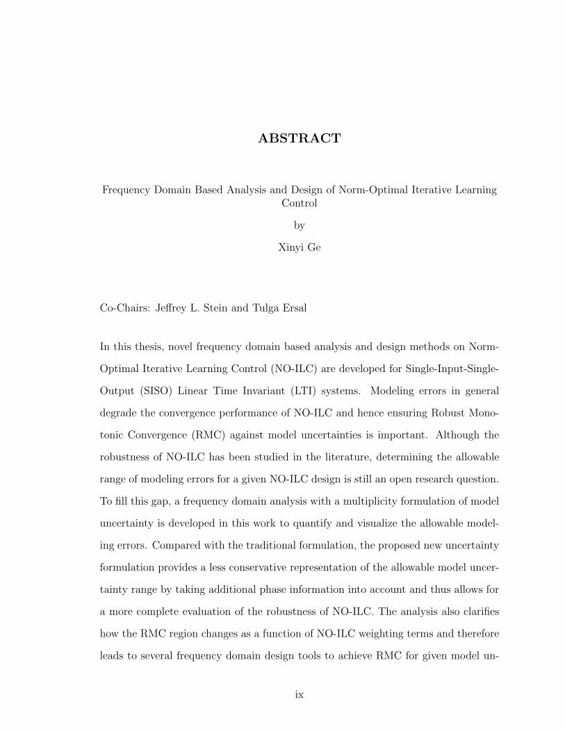
ABSTRACT

Frequency Domain Based Analysis and Design of Norm-Optimal Iterative LearningControl

by

Xinyi Ge

Co-Chairs: Jeffrey L. Stein and Tulga Ersal

In this thesis, novel frequency domain based analysis and design methods on Norm-

Optimal Iterative Learning Control (NO-ILC) are developed for Single-Input-Single-

Output (SISO) Linear Time Invariant (LTI) systems. Modeling errors in general

degrade the convergence performance of NO-ILC and hence ensuring Robust Mono-

tonic Convergence (RMC) against model uncertainties is important. Although the

robustness of NO-ILC has been studied in the literature, determining the allowable

range of modeling errors for a given NO-ILC design is still an open research question.

To fill this gap, a frequency domain analysis with a multiplicity formulation of model

uncertainty is developed in this work to quantify and visualize the allowable model-

ing errors. Compared with the traditional formulation, the proposed new uncertainty

formulation provides a less conservative representation of the allowable model uncer-

tainty range by taking additional phase information into account and thus allows for

a more complete evaluation of the robustness of NO-ILC. The analysis also clarifies

how the RMC region changes as a function of NO-ILC weighting terms and therefore

leads to several frequency domain design tools to achieve RMC for given model un-

ix

certainties. Along with this frequency domain analysis, rather than some qualitative

understanding in the literature, an equation quantitatively characterizing the funda-

mental trade-off of NO-ILC with respect to robustness, convergence speed and steady

state error at each frequency is presented, which motivates the proposed loop-shaping

like design methods for NO-ILC to achieve different performance requirements at vari-

ous frequencies. The proposed analysis also demonstrates that NO-ILC is the optimal

solution for general LTI ILC updating laws in the scope of balancing the trade-off

between robustness, convergence speed and steady state error.

x

CHAPTER I

Introduction

1.1 Brief Introduction to Iterative Learning Control

The concept of Iterative Learning Control (ILC) can be attributed to a learning

process over a repeated motion. For instance, a shooting athlete aims to shoot the

center of the target but the initial attempt is not that satisfying as shown in Fig. 1.1.

The athlete learns from this bad result and adjusts the shooting angle so that the

next attempt gives a better score. The same learning process repeats every time the

athlete makes an attempt and eventually the athlete is able to find the best shooting

angle that makes the bullet go right into the center of the target.

Similarly, ILC is a control strategy to improve the tracking performance in systems

that repeat the same operation many times. Using the tracking error and control input

from the previous iterations of the repeated motion, ILC generates the feed-forward

control signal for the subsequent iterations. In the literature, ILC is often interpreted

as feedback control in the iteration domain due to the fact that learning controller

uses the information from past trials. The standard progression in the tracking error

and control input signals over several iterations with the use of ILC is shown in Fig.

1.2. Before the start of each iteration, the ILC learning algorithms use the tracking

error and control input signals from previous iterations to generate an updated control

input signal for the current iteration to improve system performance. Ideally over

1

Figure 1.1: Shooting athlete can improve shooting accuracy by repetitive practice

several iterations, this feed-forward control input is optimized such that the tracking

error is minimized.

1.2 An Overview of ILC Literature

Since the initial proposition of ILC (Arimoto et al., 1984), a lot of theoretical

developments and application based researches have been published in the literature.

ILC has been successfully applied in areas where repetitive motions show up naturally,

for example, robotics (Arimoto et al., 1984; Oh et al., 1988; Norrlof , 2002; Tayebi ,

2004; Bouakrif et al., 2013), manufacturing (Bristow and Alleyne, 2006; Mishra et al.,

2007; Barton and Alleyne, 2008; De Roover and Bosgra, 2000; Sahoo et al., 2007) and

chemical processes (Lee et al., 2000; Gorinevsky , 2002). Recently, it has also found

applications in network-integrated systems for the purpose of eliminating communi-

cation delays, e.g., in network control systems (Pan et al., 2006; Liu et al., 2009a)

and networked hardware-in-the-loop simulations (Ersal et al., 2014; Ge et al., 2014).

After more than 30 years of development, several books (Ahn et al., 2007c; Bien

and Xu, 2012; Xu and Tan, 2003; Xu et al., 2007; Owens , 2016) and survey papers

2

Figure 1.2: A standard progression in the error and control signal over several itera-tions with the use of ILC

(Bristow et al., 2006; Ahn et al., 2007a; Xu, 2011; Li et al., 2013; Wang et al., 2009;

Lee and Lee, 2007; Longman, 2000), focusing on different aspect of ILC, have been

published, which are recommended materials as a starting point if one is particularly

interested in a certain aspect of ILC.

The inherent assumptions in ILC are the invariance of the plant dynamics (e.g.,

the initial condition, system parameters and exogenous disturbances are iteration

invariant) and the repeatability of the control task in iteration domain. The relax-

ations of these assumptions have been explored in the ILC literature. For example,

the relaxation of iteration-invariant tracking trajectory assumption can be found in

(Xu and Xu, 2004; Chi et al., 2008; Chien et al., 2008; Gao and Mishra, 2014; Al-

tin and Barton, 2015; Van Zundert et al., 2015). The handling of initial condition

shift problem in ILC is explored in (Xu and Yan, 2005; Sun and Wang , 2001, 2003;

Chi et al., 2008). The non-repetitiveness of disturbance issue has also be explored

in (Chen and Moore, 2002b; Heinzinger et al., 1992). The issue of iteration-varying

system parameters has also attracted a lot of attention for researchers and adaptive

3

ILC and high-order internal model ILC are common and effective methods to deal

with this issue (Yin et al., 2010; Chien and Yao, 2004; Choi and Lee, 2000; French

and Rogers , 2000).

Even though a large portion of the work in the ILC literature explores the first-

order ILC algorithms, (i.e., ILC updating laws that use input and tracking information

from one iteration before), high-order ILC algorithms (i.e., ILC updating laws that

use input and tracking information from more than one iterations before) have also

attracted a lot of interests in the ILC community. By incorporating more information

from previous iterations, the high-order ILC has the potential to better address the

stochastic and non-repetitive factors (Bien and Huh, 1989; Chen et al., 1998; Moore

and Chen, 2002; Phan and Longman, 2002; Norrlof and Gunnarsson, 2002b; Owens

and Feng , 2006; Hatonen et al., 2006).

Most ILC research is done in temporal domain, however, recently for specific

robotics and manufacturing applications, spatial ILC has become an active research

area to address the spatial behavior of the system (Bristow and Alleyne, 2006; Sahoo

et al., 2007; Moore et al., 2007; Cichy et al., 2011).

In terms of handling system types, ILC can be divided into two categories, i.e.,

ILC for nonlinear systems and ILC for linear systems.

For nonlinear systems, the ILC problems in general can be classified into two

categories depending on four major types (Xu, 2011): information availability, system

types, nonlinearities, design and analysis tools. The first category generally refers to

linear ILC design for globally Lipschitz continuous systems, in which output tracking

is the control objective. In this case, the system output information is available

and the relative degree is assumed to be zero, and ILC can be formulated into a

contraction mapping problem (Xu, 1997; Wang , 1998; Liu et al., 2009b; Yin et al.,

2010; Bouakrif , 2011). For the second category, nonlinear ILC updating laws are

applied to locally Lipschitz continuous systems, in which state tracking is the control

4

objective. The system state dynamics are indispensable in ILC design and analysis,

where Lyapunov approach or composite energy function approach is often used. In

this case, adaptive ILC appears as a common ILC design methodology (Chien and

Yao, 2004; Choi and Lee, 2000; French and Rogers , 2000; Tayebi , 2004; Wang et al.,

2004).

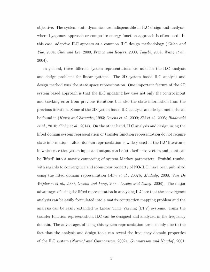
In general, three different system representations are used for the ILC analysis

and design problems for linear systems. The 2D system based ILC analysis and

design method uses the state space representation. One important feature of the 2D

system based approach is that the ILC updating law uses not only the control input

and tracking error from previous iterations but also the state information from the

previous iteration. Some of the 2D system based ILC analysis and design methods can

be found in (Kurek and Zaremba, 1993; Owens et al., 2000; Shi et al., 2005; Hladowski

et al., 2010; Cichy et al., 2014). On the other hand, ILC analysis and design using the

lifted domain system representation or transfer function representation do not require

state information. Lifted domain representation is widely used in the ILC literature,

in which case the system input and output can be ’stacked’ into vectors and plant can

be ’lifted’ into a matrix composing of system Markov parameters. Fruitful results,

with regards to convergence and robustness property of NO-ILC, have been published

using the lifted domain representation (Ahn et al., 2007b; Madady , 2008; Van De

Wijdeven et al., 2009; Owens and Feng , 2006; Owens and Daley , 2008). The major

advantages of using the lifted representation in analyzing ILC are that the convergence

analysis can be easily formulated into a matrix contraction mapping problem and the

analysis can be easily extended to Linear Time Varying (LTV) systems. Using the

transfer function representation, ILC can be designed and analyzed in the frequency

domain. The advantages of using this system representation are not only due to the

fact that the analysis and design tools can reveal the frequency domain properties

of the ILC system (Norrlof and Gunnarsson, 2002a; Gunnarsson and Norrlof , 2001;

5

Norrlof and Gunnarsson, 2005) but also due to the fact that some classical feedback

design methodologies can be leveraged into the ILC design, e.g., plant inversion (Harte

et al., 2005), H∞ and µ synthesis (De Roover and Bosgra, 2000).

1.3 Focus of This Work

This work focuses on the frequency domain analysis and design on a particular

ILC algorithm, Norm-Optimal Iterative Learning Control (NO-ILC), for Linear Time

Invariant (LTI) systems. Under the scope of LTI ILC on LTI systems, ILC design

problems can mainly be classified into four categories (Bristow et al., 2006): (1)

PD-type learning, (2) learning based on plant inversion, (3) H∞ based methods, (4)

quadratically optimal designs.

For the first category, PD-type learning (Chen and Moore, 2002a; Bristow et al.,

2006) in the iteration domain is analogous to PD control in the time domain and is one

of the widely used learning algorithms due to its ease of implementation. However,

it requires ad-hoc tuning and even though it can ensure asymptotic stability, its

transient performance may be unacceptable (Bristow et al., 2006). For the second

category, learning based on plant inversion (Bristow et al., 2006; Harte et al., 2005)

uses the inversion of the system model to update the ILC input sequence, providing

a systematic design. However, plant inversion may not work for non-minimum phase

systems. For the third category, H∞ methods (Bristow et al., 2006; De Roover and

Bosgra, 2000) offer a systematic approach to ILC design. However, all the above

mentioned design methodologies are causal and thus do not take full advantage of

the non-causal learning potential of the ILC paradigm (Donkers et al., 2008; Norrlof

and Gunnarsson, 2005; Goldsmith, 2002). For causal ILC updating laws, it has been

reported in the literature that there exist equivalent feedback realizations for causal

ILC designs (Goldsmith, 2002), therefore causal ILC updating laws are subject to

the fundamental limitations of feedback, i.e., the water-bed effect (Freudenberg and

6

Looze, 1985).

For the last category, the learning functions, so called NO-ILC, are designed in

the lifted system representation to minimize a quadratic next-iteration cost crite-

rion. NO-ILC realizes non-causal control by minimizing a cost criterion similar to

the traditional linear quadratic control concept. Due to its non-causal nature, NO-

ILC potentially has the ability to bypass the water-bed limitation and, therefore, is

gaining attention as a powerful approach. Recently, it has recently been applied to

many areas, including, but not limited to, chemical processes (Lee et al., 2000), man-

ufacturing (Barton and Alleyne, 2011; Barton et al., 2011; Janssens et al., 2013), and

networked hardware-in-the-loop simulation (Ge et al., 2014). Recognizing its advan-

tages, this thesis focuses on NO-ILC, especially on its frequency domain properties,

and develops novel frequency domain based design approaches.

In NO-ILC the learning law is synthesized via minimization of a quadratic cost

function, which was originally formulated by Amann (Amann et al., 1996) and Lee

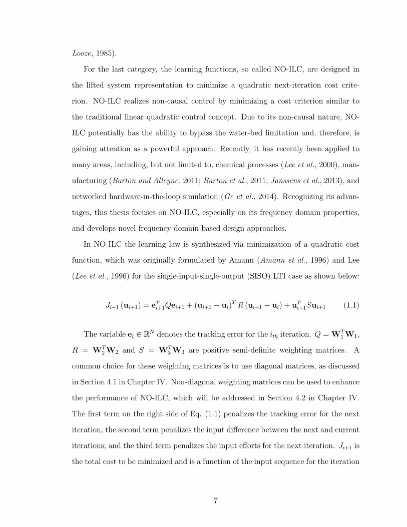
(Lee et al., 1996) for the single-input-single-output (SISO) LTI case as shown below:

Ji+1 (ui+1) = eTi+1Qei+1 + (ui+1 − ui)T R (ui+1 − ui) + uTi+1Sui+1 (1.1)

The variable ei ∈ RN denotes the tracking error for the ith iteration. Q = WT1 W1,

R = WT2 W2 and S = WT

3 W3 are positive semi-definite weighting matrices. A

common choice for these weighting matrices is to use diagonal matrices, as discussed

in Section 4.1 in Chapter IV. Non-diagonal weighting matrices can be used to enhance

the performance of NO-ILC, which will be addressed in Section 4.2 in Chapter IV.

The first term on the right side of Eq. (1.1) penalizes the tracking error for the next

iteration; the second term penalizes the input difference between the next and current

iterations; and the third term penalizes the input efforts for the next iteration. Ji+1 is

the total cost to be minimized and is a function of the input sequence for the iteration

7

i+ 1.

With the system perfectly known, asymptotic stability and monotonic stability

can be established as discussed in (Amann et al., 1996; Lee et al., 1996; Norrlof and

Gunnarsson, 2002a). Asymptotic stability guarantees the asymptotic convergence of

the tracking error, but does not provide any limits on the tracking error during the

transient phase in the iteration domain. In fact, the tracking error in this transient

phase can be large enough to make a practical implementation infeasible (Bristow

et al., 2006). Therefore, monotonic convergence is often preferred to guarantee that

the tracking error will reduce with each iteration, thereby avoiding large transient

errors. In practice, a modeling error always exists, i.e., the model used to build the

NO-ILC updating law is always different from the real system due to, for example, un-

modeled dynamics. This modeling error can be estimated or identified to be within

a certain range, but is in general not known exactly. Since NO-ILC is a model-based

approach, modeling errors can degrade its performance. Therefore, the robustness of

NO-ILC is an important topic and is one of the main focuses of this work.

Robustness of ILC algorithms in general has been subject to prior research. In

(Ahn et al., 2005, 2007b), the Schur stability radius in designing a general robust

ILC has been investigated, assuming there exist interval uncertainties in the Markov

parameters of the systems. However, this approach leads to conservative results with

respect to the stipulated model uncertainty. In (Harte et al., 2005; Owens et al., 2009),

the Robust Monotonic Convergence (RMC) of inverse-based ILC and gradient-based

ILC has been studied. However, these algorithms are only special forms of NO-ILC

and can only handle positive real modeling errors due to the absence of Q-filters. In

(Van De Wijdeven et al., 2009), the RMC of finite time interval ILC is investigated.

In particular, µ analysis is adopted to check the RMC condition for ILC with an

uncertainty formulation. For a given upper bound on the model uncertainty and a

given ILC design, this tool provides a means for checking RMC.

8

For the specific context of NO-ILC, the RMC has been studied to a certain degree

in the literature (Donkers et al., 2008; Gorinevsky , 2002; Van De Wijdeven et al.,

2009; Owens , 2016). Specifically, RMC criteria in both time and frequency domain

have been derived, based on which numerous design and tuning approaches have been

proposed. However, determining the allowable range of modeling error for a given

NO-ILC design is not a research question that has been fully answered. Even though

the existing tools can be utilized in an attempt to answer this question, this would

not only require a trial-and-error process, but also give conservative evaluations of

the RMC range. This would lead to a conservative filter design for NO-ILC in terms

of convergence speed and steady state tracking error; i.e., convergence speed may be

unnecessarily slow or an unnecessary steady state tracking error may be introduced.

Therefore, it is important to know how the range of the allowable modeling error

is affected by the weighting terms in the cost function of NO-ILC to enable more

aggressive designs against modeling uncertainties.

Besides robustness, as mentioned above, convergence speed and steady state error

are also important concerns since a too robust solution leading to poor convergence

speed or unnecessary steady state error is not preferred. For the convergence speed,

inverting the plant, i.e., setting R = 0 and S = 0 in Eq. (1.1), in general achieves

the fastest convergence speed, since theoretically the ILC output convergences after

one iteration of learning. However, this method is usually not feasible due to the

existence of model uncertainties as well as the non-minimum phase nature of some

systems.

As for the steady state error, the trade-off between steady state error and ro-

bustness has been addressed in the literature qualitatively: increasing S provides

additional robustness at the expense of a larger steady state error (Donkers et al.,

2008; Gorinevsky , 2002). However, due to the specific uncertainty formulation used,

it has been reported that R does not affect the robustness of NO-ILC (Donkers et al.,

9

2008; Gorinevsky , 2002).

The work reviewed so far focuses on the problem of analyzing the RMC, conver-

gence speed, or steady state error of NO-ILC for a given design of weighting matrices.

The dual problem, i.e., the design and tuning of NO-ILC weighting matrices for a

desired level of robustness, convergence speed, or steady state error has also been

subject to prior investigation. However, majority of the design and tuning tools use

diagonal matrices (Gunnarsson and Norrlof , 2001; Bristow , 2008; Lee et al., 2000;

Donkers et al., 2008), which limits the design freedom in adjusting the trade-off be-

tween robustness, convergence speed, and steady state error. In (Gorinevsky , 2002),

a loop shaping technique is proposed to address the design of a non-diagonal S matrix

to balance the robustness and steady state error trade-off. Other design and tuning

methods using time varying weighting matrices have also been proposed (Barton and

Alleyne, 2011).

In light of this literature review, several gaps are identified.

• An analysis tool that completely evaluates the allowable model uncertainties

against the NO-ILC weighting matrices has not been fully developed.

• A design technique that allows for the design of NO-ILC according to different

robustness, convergence speed and steady state error requirements at different

frequencies does not yet exist.

• An analytical equation that quantitatively characterizes the fundamental trade-

off between robustness, convergence speed and steady state error has not yet

been established.

The objective of this research is to provide fundamental analysis tools for the

frequency domain properties of NO-ILC, which leads to novel design methodologies

for NO-ILC to adjust the trade-off between robustness, convergence speed and steady

state error at different frequencies.

10

1.4 Thesis Contributions and Outline

Through an infinite time horizon analysis, the main contributions of this work can

be summarized as follows:

• This work presents a new model uncertainty formulation for NO-ILC. Unlike

the conventional uncertainty formulation, which leads to the conclusion that R

does not affect the robustness (Donkers et al., 2008; Gorinevsky , 2002), the new

formulation used in this work yields that the robustness is affected by both R

and S but in different manners.

• Based on the above uncertainty formulation, this work both mathematically

and graphically presents how the weighting terms in the cost function affect the

robustness of NO-ILC. This leads to several new graphical design methodologies

for the weighting matrices to achieve the RMC requirement.

• An analytical equation is derived to quantitatively characterize the fundamental

trade-off between robustness, convergence speed and steady state error of NO-

ILC in frequency domain. This equation can be helpful during the design process

to satisfy a desired robustness requirement while ensuring fast convergence and

small steady state error at different frequencies. This equation also reveals the

optimality of NO-ILC among general ILC updating laws in the scope of LTI

systems.

• Based on the analysis on allowable model uncertainty and fundamental trade-off

for NO-ILC, two optimization based formulations are proposed to systematically

design the weighting matrices for NO-ILC, which eliminate the manual tuning

process and avoid unnecessarily conservative designs.

The rest of this thesis is organized as follows: Chapter II reviews the background

of NO-ILC, including different system representations, derivation of the NO-ILC up-

11

dating law, definition of monotonic convergence and formulation of modeling error.

Chapter III discusses the proposed model uncertainty formulation and how this un-

certainty is visualized on the Bode and Nyquist plots. Then the frequency domain

Robust Monotonic Convergence (RMC) criterion is revisited and the its validity to-

wards infinite time horizon is addressed. Chapter IV presents two novel RMC analysis

and design tools for NO-ILC, one with diagonal weighting matrices design and the

other one with frequency dependent weighting matrices design. Both analysis meth-

ods offer graphical interpretations of the allowable model uncertainty region on the

Nyquist plot and lead to novel design guidelines. Chapter V develops an analytical

equation that characterizes the fundamental trade-off of NO-ILC between robustness,

convergence speed and steady state error at each frequency. In addition, the chapter

demonstrates that NO-ILC is the optimal solution under the scope of general LTI ILC

updating laws for LTI systems in terms addressing the trade-off between robustness,

convergence speed and steady state error at each frequency. Chapter VI presents two

different formulations for the design of NO-ILC weighting matrices as an optimization

problem to eliminate the manual tuning process and avoid unnecessarily conservative

designs. Chapter VII summarizes the contributions of this thesis and lays out several

potential future research directions.

12

CHAPTER II

Background of NO-ILC

In this chapter, background of NO-ILC is reviewed. First, three different system

realizations and the transformations between them are presented. Next, the derivation

of the NO-ILC updating law in the lifted domain is reviewed. Then, monotonic

convergence and modeling error are discussed. Finally, the frequency domain NO-

ILC updating law is presented.

2.1 System Representation

Consider a discrete SISO LTI system with the following state-space realization:

xi(t+ 1) = Axi(t) +Bui(t)

yi(t) = Cxi(t) +Dui(t)

(2.1)

The matrices A, B, C, D are assumed to be time and iteration invariant. The

variables i ∈ [0, k] and t ∈ [0, N−1] denote the iteration and time index, respectively,

with N being the number of time steps in each iteration. The state variables, inputs

and outputs are given by xi(t) ∈ Rn, ui(t) ∈ R, yi(t) ∈ R, respectively, where n

denotes the number of state variables.

Beside the state-space realization, the transfer function realization can also be

13

used to represent a LTI system:

yi(z) = G(z)ui(z) + d(z) (2.2)

Here, yi(z) and ui(z) are the z-transforms of the control output and input of the sys-

tem, respectively. G(z) is a rational transfer function and is equal to C(zI − A)−1B+

D. d(z) is the z-transform of the free response.

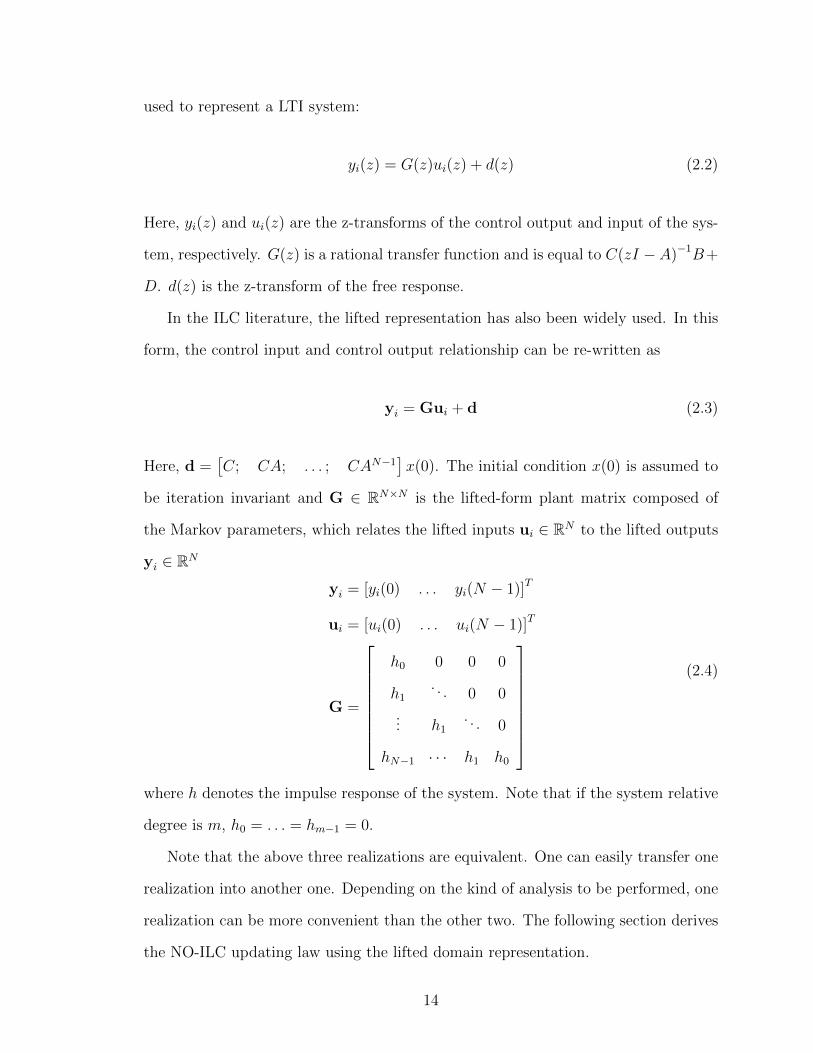
In the ILC literature, the lifted representation has also been widely used. In this

form, the control input and control output relationship can be re-written as

yi = Gui + d (2.3)

Here, d =[C; CA; . . . ; CAN−1

]x(0). The initial condition x(0) is assumed to

be iteration invariant and G ∈ RN×N is the lifted-form plant matrix composed of

the Markov parameters, which relates the lifted inputs ui ∈ RN to the lifted outputs

yi ∈ RN

yi = [yi(0) . . . yi(N − 1)]T

ui = [ui(0) . . . ui(N − 1)]T

G =

h0 0 0 0

h1. . . 0 0

... h1. . . 0

hN−1 · · · h1 h0

(2.4)

where h denotes the impulse response of the system. Note that if the system relative

degree is m, h0 = . . . = hm−1 = 0.

Note that the above three realizations are equivalent. One can easily transfer one

realization into another one. Depending on the kind of analysis to be performed, one

realization can be more convenient than the other two. The following section derives

the NO-ILC updating law using the lifted domain representation.

14

2.2 Derivation of NO-ILC Updating Law

The control goal of NO-ILC is to find the input sequence so that the total cost

shown in Eq. (1.1) is minimized. This can be done by setting ∂Ji+1∂ui+1

= 0, which

translates to the following updating law:

ui+1 = Qui + Lei (2.5)

where the so-called Q-filter Q ∈ RN×N and the learning gain L ∈ RN×N are given by

(Amann et al., 1996; Lee et al., 1996)

Q = (GToQGo +R + S)−1(GT

oQGo +R)

L = (GToQGo +R + S)−1GT

oQ

(2.6)

where Go ∈ RN×N is the lifted domain representation of the nominal plant. Weighting

matrices Q, R and S not only provide the design freedom to ensure convergence of the

NO-ILC in the presence of plant uncertainties but also affect the convergence speed

and steady state tracking error performance of NO-ILC, which are addressed in later

chapters.

2.3 Monotonic Convergence

One property of interest is the monotonic convergence, i.e., the tracking perfor-

mance is improved every time the experiment is repeated. Monotonic convergence

can be analyzed from the tracking error dynamics in the iteration domain:

ei+1 = yd − yi+1 = yd −Gui+1 = yd −G (Qui + Lei)

= yd −GQG−1Gui −GLei

= yd −GQG−1 (yd − ei)−GLei

(2.7)

15

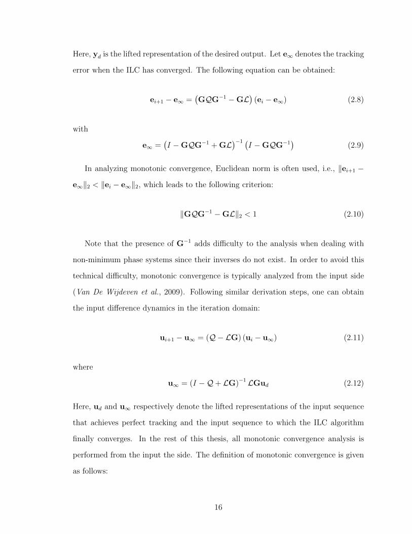
Here, yd is the lifted representation of the desired output. Let e∞ denotes the tracking

error when the ILC has converged. The following equation can be obtained:

ei+1 − e∞ =(GQG−1 −GL

)(ei − e∞) (2.8)

with

e∞ =(I −GQG−1 + GL

)−1 (I −GQG−1

)(2.9)

In analyzing monotonic convergence, Euclidean norm is often used, i.e., ‖ei+1 −

e∞‖2 < ‖ei − e∞‖2, which leads to the following criterion:

‖GQG−1 −GL‖2 < 1 (2.10)

Note that the presence of G−1 adds difficulty to the analysis when dealing with

non-minimum phase systems since their inverses do not exist. In order to avoid this

technical difficulty, monotonic convergence is typically analyzed from the input side

(Van De Wijdeven et al., 2009). Following similar derivation steps, one can obtain

the input difference dynamics in the iteration domain:

ui+1 − u∞ = (Q−LG) (ui − u∞) (2.11)

where

u∞ = (I −Q+ LG)−1 LGud (2.12)

Here, ud and u∞ respectively denote the lifted representations of the input sequence

that achieves perfect tracking and the input sequence to which the ILC algorithm

finally converges. In the rest of this thesis, all monotonic convergence analysis is

performed from the input the side. The definition of monotonic convergence is given

as follows:

16

G

(z)e

U (z)oG

(z)iu (z)iy

(z)G

(a) (b)

oG

eUiu iy

Figure 2.1: Formulation of modeling error in the (a) time and (b) frequency domain

Definition II.1. The ILC system is monotonic convergent from the input side if

‖ui+1−u∞‖2 < ‖ui−u∞‖2 for all i ∈ [1, k] and for any desired output trajectory yd.

Therefore, the necessary and sufficient condition for monotonic convergence from

the input side naturally follows:

‖Q − LG‖2 < 1 (2.13)

2.4 Modeling Error

In a real control application, the exact lifted-form plant matrix, G, is always

unknown due to some modeling error. The available information is the nominal plant,

Go, and possibly the range of the modeling error. To investigate the robustness of

the NO-ILC algorithm, modeling error is incorporated as shown in Fig. 2.1 (Owens

et al., 2009; Harte et al., 2005).

Proposition II.2. Both Ue and Ue(z) denote the modeling error, which represent a

stable causal LTI SISO system. The relative degree of Go(z) is assumed to be smaller

than or equal to that of G(z), with G(z) = Ue(z)Go(z). If G, Go and Ue are lifted

matrix representations of these systems, then G = UeGo.

In the presence of modeling error, plugging G = UeGo into Eq. (2.13), the Robust

Monotonic Convergence (RMC) criterion is shown as following:

‖Q − LUeGo‖2 < 1 (2.14)

17

2.5 NO-ILC in Frequency Domain

Instead of analyzing the updating law in the time domain, this thesis performs

an analysis in the frequency domain. Frequency domain analysis has been a well-

established tool in the literature (Donkers et al., 2008; Gorinevsky , 2002; Gunnarsson

and Norrlof , 2001; Norrlof and Gunnarsson, 2002a, 2005) for infinite time horizon

analysis, i.e., N → ∞, and is adopted in this work as well to provide insights about

the performance of NO-ILC that can be useful in determining the weighting matrices

for NO-ILC. This thesis considers LTI systems; therefore, W1, W2 and W3 can be

considered as lifted representations of LTI filters. Thus, for the remainder of this

work, the following frequency-domain updating law is considered:

ui+1(z) = Q(z)ui(z) + L(z)ei(z)

Q(z) =Go(z

−1)Q(z)Go(z) +R(z)

Go(z−1)Q(z)Go(z) +R(z) + S(z)

L(z) =Go(z

−1)Q(z)

Go(z−1)Q(z)Go(z) +R(z) + S(z)

(2.15)

where weighting filters Q(z) = W1(z−1)W1(z), R(z) = W2(z−1)W2(z) and S(z) =

W3(z−1)W3(z) are zero phase filters and W1(z), W2(z) and W3(z) are causal LTI

filters.

Note here Q, L, Q, R, S and GTo are just lifted representations of Q(z), L(z),

Q(z), R(z), S(z) and Go(z−1). These notations are frequently used in the rest of the

thesis.

18

CHAPTER III

Model Uncertainty Formulation

In this chapter, a new model uncertainty formulation is proposed. Given the upper

and lower bounds of uncertainty, the uncertainty region on the Bode plot is transferred

to the Nyquist plot. Then, the frequency domain RMC criterion is revisited, where

its validity is addressed and the shortcomings of the existing graphical interpretation

are laid out.

3.1 Model Uncertainty

The modeling error Ue(z) is in general unknown, but belongs to a certain range,

which can be estimated or obtained, for example, through frequency response tests.

The following paragraphs discuss the uncertainty range transformation between the

Bode plot and Nyquist plot.

Fig. 3.1 shows the frequency response of the nominal plant (indicated as the solid

green curve) and the upper/lower bounds of model uncertainty region (indicated

as the dashed blue curves, denoted as Gmax(z) = Ue,max(z)Go(z) and Gmin(z) =

Ue,min(z)Go(z)). Thus, the real system G(z) = Ue(z)Go(z) can be any curve within

19

-150

-100

-50

0

10-1

100

101

102

103

104

-270

-225

-180

-135

-90

-45

0

Mag

nit

ude

(dB

)P

has

e (d

eg)

Frequency (rad/s)

Uncertainty Bounds

System Model

Uncertainty Range

1ω

1ω

2ω

2ω

( )maxG z

( )minG z

Figure 3.1: Example model uncertainty expressed on the Bode plot

the shaded region. Therefore, the following relationships hold:

∣∣Ue,min

(ejθ)∣∣ ≤ ∣∣Ue (ejθ)∣∣ ≤ ∣∣Ue,max

(ejθ)∣∣

]Ue,min

(ejθ)≤]Ue

(ejθ)≤]Ue,max

(ejθ) (3.1)

where |·| and ] denote the magnitude and phase of a complex number, respectively.

θ = Tsω, where Ts is the time step size and ω is the frequency.

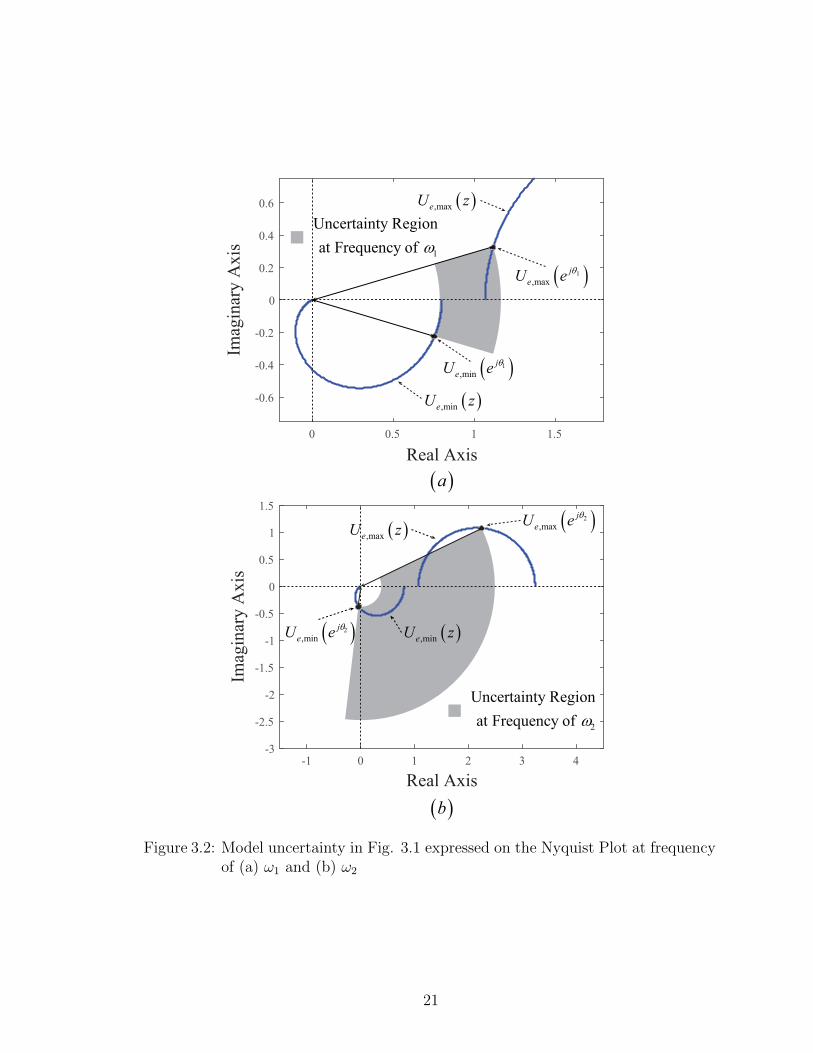
At each frequency ω, according to Eq. (3.1), the range of Ue(ejθ) can be interpreted

on the Nyquist plot. As an example, the model uncertainty regions corresponding to

the two frequencies ω1 and ω2 shown in Fig. 3.1 are shown as the gray regions in Fig.

3.2.

The novelty of the proposed uncertainty formulation and its significance can be

stated in detail as follows. The robust control literature proposes the uncertainty

formulation G(z) = Go(z)(1 + wI(z)∆(z)), where wI(z) is the weighting for uncer-

tainty and |∆(z)|∞ ≤ 1. Here |·|∞ denotes the H∞ norm. This formulation, which

incorporates magnitude information only, has been widely adopted into the ILC lit-

20

0 0.5 1 1.5

-0.6

-0.4

-0.2

0

0.2

0.4

0.6

Real Axis

Imag

inar

y A

xis

-1 0 1 2 3 4-3

-2.5

-2

-1.5

-1

-0.5

0

0.5

1

1.5

Imag

inar

y A

xis

Real Axis

( )a

( )b

( )1

,min

j

eU eθ

( )1

,max

j

eU eθ

( ),mineU z

( ),maxeU z

( )2

,max

j

eU eθ

( )2

,min

j

eU eθ

( ),maxeU z

( ),mineU z

2

Uncertainty Region

at Frequency of ω

1

Uncertainty Region

at Frequency of ω

Figure 3.2: Model uncertainty in Fig. 3.1 expressed on the Nyquist Plot at frequencyof (a) ω1 and (b) ω2

21

erature. It represents an uncertainty region in the Nyquist plot that is a disk cen-

tered at (1, 0) with a radius of∣∣wI(ejθ)∣∣ at each frequency. Using the uncertainty

formulation of G(z) = Go(z)(1 + wI(z)∆(z)) leads to the conclusion that the term

(ui+1 − ui)T R (ui+1 − ui) in the NO-ILC cost function, Eq. (1.1), does not affect the

robustness of NO-ILC (Gorinevsky , 2002; Donkers et al., 2008). The proposed un-

certainty formulation in this thesis incorporates not only the magnitude information

but also the phase information. With this proposed uncertainty formulation, it is

shown that the term (ui+1 − ui)T R (ui+1 − ui) in Eq. (1.1) actually affects the RMC

region, but in a different manner compared with the term uTi Qui (details are given

in Chapter IV). Also, given the upper and lower bounds for the uncertainty region

shown in Fig. 3.1, using G(z) = Go(z)(1 + wI(z)∆(z)) leads to a more conservative

uncertainty region representation on the Nyquist plot compared with the proposed

one, since using this traditional uncertainty formulation to represent the proposed

uncertainty shown in Fig. 3.1 leads to an uncertainty region that is a disk centered

at (1, 0) with radius of∣∣wI(ejθ)∣∣ that encloses the gray region in Fig. 3.2.

As an example, consider the model uncertainty shown in Fig. 3.1 at the frequency

of ω2. Using the proposed uncertainty formulation leads to an uncertainty region

shown as the dark gray region in Fig. 3.3. Using the traditional uncertainty formula-

tion, G(z) = Go(z)(1 +wI(z)∆(z)), leads to an uncertainty region shown as the light

gray disk in Fig. 3.3. The proposed uncertainty formulation incorporates both mag-

nitude and phase information, while the traditional uncertainty formulation just uses

the magnitude information. Thus, the proposed formulation leads to a less conserva-

tive uncertainty region representation. How this helps to achieve a less conservative

robust monotonic convergent NO-ILC design is discussed in Chapter IV.

22

-2 0 2 4 6-4

-3

-2

-1

0

1

2

3

4

Real Axis

Imag

inar

y A

xis

1

( )2j

Iw e

θ

( ),maxeU z

( ),maxeU z

( )2

,min

j

eU e

θ

( ),mineU z Proposed

Formulation

Traditional

Formulation

Figure 3.3: Comparison of the proposed and traditional model uncertainty formula-tions

3.2 Frequency Domain RMC Criterion

This work focuses on an infinite time horizon analysis, i.e., N → ∞. For an

infinite time horizon, the following monotonic convergence criterion has been widely

used in the literature:

|Q(z)−G(z)L(z)|∞ < 1 (3.2)

This criterion was originally proven in (Norrlof and Gunnarsson, 2002a) for causal

Q(z) and L(z) and has also been stated as an appropriate convergence criterion for

infinite time horizon analysis in the literature for NO-ILC (Gunnarsson and Norrlof ,

2001; Donkers et al., 2008), which has non-causal Q(z) and L(z). A detailed discus-

sion on the validity of the above frequency domain monotonic convergence criterion

for an infinite time horizon analysis is shown in the coming paragraphs. The differ-

ence between the time and frequency domain non-causal ILC updating law is pointed

out first for the infinite time horizon case. Then, the validity of using Eq. (3.2) as

23

N

1( )iu z

+ 1i+u

Figure 3.4: An illustration of ui+1 and ui+1(z) obtained through Eq. (3.3)

the RMC criterion for an infinite time horizon analysis of NO-ILC is discussed.

Recall that the input for the next iteration ui+1 and ui+1(z) are obtained through

the following updating laws:

ui+1 = Qui + Lei

ui+1(z) = Q(z)ui(z) + L(z)ei(z)

(3.3)

where Q and L are the lifted representations of the non-causal Q(z) and L(z). One

important difference between ui+1 and ui+1(z) is the fact that ui+1 denotes a signal

that only exists in the positive time interval, whereas ui+1(z) denotes a signal that has

components in the negative time interval, as well, since Q(z) and L(z) are non-causal.

This difference is illustrated in Fig. 3.4. For the rest of this section, Z{·} and Z−1{·}

are used to denote the two sided z-transform and inverse z-transform of a signal. For

a signal, the notation g denotes only its causal portion, while g(z) denotes the two

sided z-transform of this signal. Thus, Z{g} is not equal to g(z) unless the signal is

causal.

Monotonic convergence is defined as ‖ui+1 − u∞‖2 < ‖ui − u∞‖2. The input and

tracking error from the current iteration must be causal signals, since these are the

signals collected from a physical system. Thus, ui(z) = Z{ui} and ei(z) = Z{ei}.

Using Parseval’s Theorem, it is straightforward to show that Eq. (3.2) is the

criterion for Eq. (3.4).

∥∥Z−1{ui+1(z)} − Z−1{u∞(z)}∥∥

2<∥∥Z−1{ui(z)} − Z−1{u∞(z)}

∥∥2

(3.4)

24

Eq. (3.4) indicates that ui+1(z) will monotonically converge to u∞(z). However,

once ui+1(z) is truncated into ui+1, is Eq. (3.2) still an appropriate monotonic con-

vergence criterion for the non-causal ILC updating laws in the infinite time horizon

analysis?

When Q (z) = 1, it can be shown that Eq. (3.2) is a valid criterion for ‖ui+1 −

u∞‖2 < ‖ui − u∞‖2. To this end, the causality of u∞(z) plays a critical role.

Let ud(z) be the causal and stable ideal input sequence that can go through the

physical system G(z) so that G(z)ud(z) = r(z), where r(z) is the tracking reference.

u∞(z) is the input sequence when the algorithm converges and it can be derived from

Eq. (3.3) as follows:

u∞(z) =G(z)L(z)

1−Q(z) +G(z)L(z)ud(z) (3.5)

For NO-ILC, when Q(z) = 1, u∞(z) is causal since u∞(z) = ud(z) from the above

equation and ud(z) is causal. When Q(z) 6= 1, u∞(z) becomes non-causal.

In the case when u∞(z) is causal, i.e., Q(z) = 1 for NO-ILC, since ui(z) is causal,

too, as discussed in the previous section, Eq. (3.4) can be rewritten into

∥∥Z−1{ui+1(z)} − u∞∥∥

2< ‖ui − u∞‖2 (3.6)

Since the signal ui+1−u∞ is the causal portion of the signal Z−1{ui+1(z)} − u∞, the

following relationship is true:

‖ui+1 − u∞‖2 ≤∥∥Z−1{ui+1(z)} − u∞

∥∥2

(3.7)

Therefore,

‖ui+1 − u∞‖2 ≤∥∥Z−1{ui+1(z)} − u∞

∥∥2< ‖ui − u∞‖2 (3.8)

Thus, Eq. (3.2) is the criterion for ‖ui+1−u∞‖2 < ‖ui−u∞‖2 when u∞(z) is causal,

25

i.e., Q (z) = 1.

When Q (z) 6= 1, Eq. (3.2) can be used as an approximation for an infinite time

horizon analysis according to the following argument. The small portion of the signal

that lies in the negative time interval (the portion of the blue curve that lies in the

negative time interval in Fig. 3.4) can be neglected since the portion in the positive

time interval will dominate when N → ∞. Thus, Eq. (3.2) can be an appropriate

monotonic convergence criterion for non-causal ILC updating laws for the infinite time

horizon analysis, if one is mindful of the fact that NO-ILC is always implemented in

a finite time horizon. In particular, since the analysis is performed in the infinite

time horizon, it is reasonable to expect some errors at the beginning and end of each

iteration. The errors at the beginning are due to the fact that the non-causal portion

of ui+1(z) is truncated, since inputs in the negative time interval cannot be fed to a

physical system. The errors at the end are due to the fact that the time does not go

to infinity. Nevertheless, when N is sufficiently large, the frequency domain analysis

provides a good approximation of time domain results.

As a conclusion, for NO-ILC, when Q(z) = 1, Eq. (3.2) can be rigorously jus-

tified as a valid RMC criterion for infinite time horizon analysis. Otherwise, Eq.

(3.2) should be used as an approximation. As the time horizon becomes larger, this

approximation becomes better, because the signals in the positive time interval will

dominate the signals in the negative time interval.

It is very important to note that, in practice, NO-ILC is always implemented in

finite time horizon. The time domain convergence criterion is ||Q − LG||2 < 1. It

has been pointed out in (Van De Wijdeven et al., 2009) that the frequency domain

convergence criterion, Eq. (3.2), implies the time domain convergence criterion only

when L(z) is causal. For NO-ILC, however, the learning gain L(z) is non-causal.

Thus, Eq. (3.2) can only be used as an approximation since the time horizon is

always finite in practice. Nevertheless, the frequency domain interpretation still gives

26

useful insights in terms of designing NO-ILC when N is sufficiently large, i.e, the time

horizon is significantly longer than the length of the non-zero impulse responses of

G(z), W1(z), W2(z) and W3(z). For example, among all the simulation tests that the

author has performed to date, a value of N that is five times longer than the length

of the non-zero impulse responses of all the filters, the frequency domain analysis and

design approach served as a good approximation.

Therefore, it would be prudent to leave some safety margin and not design the

RMC disk, which will be discussed in Chapter IV, too tight around the uncertain

region on the Nyquist plot.

3.3 Existing Graphical Interpretation on RMC

Substituting the uncertainty formulation, G(z) = Ue(z)Go(z), and NO-ILC up-

dating law, Eq. (2.15), into the monotonic convergence criterion, Eq. (3.2), the

following expression can be obtained for all θ ∈ [0, 2π]:

∣∣∣∣∣1−∣∣W1

(ejθ)∣∣2∣∣Go

(ejθ)∣∣2

|W1 (ejθ)|2|Go (ejθ)|2 + |W2 (ejθ)|2Ue(ejθ)∣∣∣∣∣

< 1 +

∣∣W3

(ejθ)∣∣2

|W1 (ejθ)|2|Go (ejθ)|2 + |W2 (ejθ)|2(3.9)

Note that Ue(ejθ) is a complex number; worst case scenario of Eq. (3.9) for a

particular θ in the complex plane is shown in Fig. 3.5. With modeling error Ue(z),

the causal LTI filters, W1(z),W2(z) and W3(z), should be chosen so that the green

vector in Fig. 3.5 lies within the red circle.

This graphical interpretation helps with the qualitative understanding of the ro-

bustness of NO-ILC; similar interpretations can be found in (Gunnarsson and Nor-

rlof , 2001; Norrlof and Gunnarsson, 2005). However, using the above interpretation

to design or tune a robust monotonic convergent NO-ILC is a challenge for the fol-

27

Re1

Im

( ) ( )

( ) ( ) ( )( )

2 2

2 2 2

1

1 2

1j

e

j j

o

j j j

o

W e G e

W e G

U e

e W e

θ θ

θ

θ θ θ

−

+

( )

( ) ( ) ( )

2

2

3

1

2

2

21

j

j j j

o

W e

W e G e W e

θ

θ θ θ

+

+

Figure 3.5: Graphical interpretation of Eq. (3.9)

lowing reasons. In real applications, the modeling error Ue(z) is not known exactly,

but only its range is known. Hence, Fig. 3.5 must include not only one, but a set

of vectors that cover the modeling error range. Furthermore, the appearance of Fig.

3.5 depends on W1(z), W2(z), W3(z), Go(z) and Ue(z). This implies two challenges.

First, a new figure must be created for each frequency. Second, because both the

radius of the circle and the vectors depend on the NO-ILC design parameters W1(z),

W2(z) and W3(z), the radius of the circle and the vectors cannot be adjusted inde-

pendently. Because of these reasons, using the graphical interpretation in Fig. 3.5

for design would lead to an ad-hoc and time consuming process.

Therefore, a new graphical interpretation is needed that decouples the complex

geometric interdependencies in Fig. 3.5 and helps visualize what the allowable range

of modeling error for RMC is for a specific design of W1(z), W2(z) and W3(z). The

following chapter addresses this gap using a frequency domain analysis.

On the other hand, from analysis in the time domain, the RMC criterion is pro-

posed in (Donkers et al., 2008; Van De Wijdeven et al., 2009). The results in (Van De

Wijdeven et al., 2009) are useful for checking RMC for specific model uncertainties and

28

ILC filter designsQ(z) and L(z). However, no design guidelines are suggested. Hence,

using this tool to address the gap identified above would require a trial-and-error pro-

cess of applying RMC criterion to various W1(z), W2(z) and W3(z) designs until a

design that yields a satisfactory performance is found. Furthermore, the argument in

(Donkers et al., 2008; Gorinevsky , 2002) has stated that (ui+1 − ui)T R (ui+1 − ui) in

Eq. (1.1) does not influence the RMC properties of NO-ILC. However, through the

analysis in this thesis, a stronger statement is obtained; namely, increasing R influ-

ences RMC positively. Hence, the existing techniques give a conservative evaluation

of the RMC range, whereas the analysis provided in this work aims to provide a more

complete evaluation, as well as a less conservative systematic design process.

3.4 Conclusion

In this chapter, a new model uncertainty formulation is proposed. Unlike the

traditional uncertainty formulation which does not incorporate the phase information,

the proposed uncertainty formulation incorporates both the magnitude and phase

information. The incorporation of this additional phase information not only provides

a less conservative representation of the uncertainty region but also, more importantly,

leads to a more aggressive NO-ILC design as discussed in the next chapter.

The proposed uncertainty formulation is initially formulated on the Bode plot.

This chapter presents a method to transfer the uncertainty region from the Bode plot

to the Nyquist plot at each frequency. Then the frequency domain RMC criterion

is revisited. The validity of this criterion is addressed for the infinite time horizon

analysis. Even though this frequency domain RMC criterion is only an approximation

since NO-ILC is always implemented in finite time horizon, the infinite time horizon

analysis still provides useful insights towards some frequency domain properties of

NO-ILC. Finally, the shortcomings of the existing graphical interpretation are laid

out, which motivates new frequency domain analysis and design methodologies for

29

NO-ILC.

30

CHAPTER IV

RMC Analysis and Design Tools

In this chapter, the frequency domain RMC analysis and design methodologies are

addressed. New graphical interpretations that characterize the allowable modeling

errors for NO-ILC are presented, with the understanding of which the RMC design

guidelines naturally follow. The discussions can be divided into two parts.

For the first part, Section 4.1, diagonal weighting matrices analysis and design

methodologies for NO-ILC are addressed. Setting the weighting matrices Q, R and

S to I, λI and βI respectively, where I denotes the identity matrix, and adjusting

the λ and β values for the RMC requirement is a common choice when designing

NO-ILC. With respect to the equivalent frequency domain realization, this indicates

W1(z) = 1, W2(z) =√λ and W3(z) =

√β. In this part, the allowable modeling

error region on the Nyquist plot is characterized with and without the Q-filter. Then

a design guideline is proposed. Finally, some simulation examples are presented to

demonstrate the utility of the theoretical results.

For the second part, Section 4.2, the analysis and design methodologies for non-

diagonal weighting matrices for NO-ILC are addressed. Unlike the previous case in

which W1(z), W2(z) and W3(z) are just constant gains, the magnitudes of∣∣W1

(ejθ)∣∣,∣∣W2

(ejθ)∣∣ and

∣∣W3

(ejθ)∣∣ are adjusted at different frequencies. This leads to a fre-

quency dependent weighting matrices design. Compared with the previous design

31

approach discussed in Section 4.1, this frequency dependent design approach bet-

ter addresses the fundamental trade-off between robustness, convergence speed and

steady state error, which is discussed in Chapter V. First, the effect of the weighting

filters W1(z), W2(z) and W3(z) affect the RMC region on the Nyquist plot is dis-

cussed. Then design guidelines for this approach are proposed, followed with some

simulation examples.

4.1 Diagonal Weighting Matrices Design

In this section, the allowable region of the modeling error Ue(z) is interpreted

through the Nyquist plot for a robust monotonic convergent NO-ILC as a function

of λ and β. Before going into the detailed analysis, note that, with W1(z) = 1,

W2(z) =√λ and W3(z) =

√β, Eq. (3.2) can be re-written into Eq. (4.1) for all

θ ∈ [0, 2π], where Re{·} denotes the real part of a complex number. From now on,

Eq. (4.1) serves as the criterion for RMC and the following two sections discuss the

interpretation of this criterion with β = 0 and β 6= 0; i.e., with and without the

Q-filter.

( ∣∣Go

(ejθ)∣∣2

|Go (ejθ)|2 + λ+ β

)2∣∣Ue (ejθ)∣∣2 +

( ∣∣Go

(ejθ)∣∣2 + λ

|Go (ejθ)|2 + λ+ β

)2

− 2

(∣∣Go

(ejθ)∣∣2 + λ

) ∣∣Go

(ejθ)∣∣2

|Go (ejθ)|2 + λ+ βRe{Ue

(ejθ)} < 1 (4.1)

4.1.1 RMC of NO-ILC without Q-Filter

In this section, the allowable modeling error region is analyzed for the RMC

condition. With the Q-filter disabled, the corresponding allowable error with respect

to a specific λ value is illustrated visually on the Nyquist plot. The results show that

the RMC region expands as λ increases, but there are certain modeling errors that

cannot be accommodated with using λ only.

32

With β = 0, Criterion (4.1) can be simplified as follows. For all θ ∈ [0, 2π]

α2 (θ)∣∣Ue (ejθ)∣∣2 − 2α (θ) Re{

(Ue(ejθ))} < 0 (4.2)

where α (θ) is defined as

α (θ) ,

∣∣Go

(ejθ)∣∣2

|Go (ejθ)|2 + λ∈ (0, 1] (4.3)

Proposition IV.1. The NO-ILC with the updating law of Eq. (2.15) with β = 0

cannot be robust monotonic convergent for the uncertain plant formulated in Propo-

sition II.2, if Re{Ue(ejθ)} is negative for any θ ∈ [0, 2π].

Proof. See Appendix A for the proof.

The above proposition illustrates the fundamental limitation of using only λ. If

Re{Ue(ejθ)} is negative for any θ ∈ [0, 2π], it is not possible to satisfy Criterion (3.2)

by using λ only. Nevertheless, increasing λ still helps enlarge the RMC region as

discussed below.

Proposition IV.2. With the updating law of Eq. (2.15), if NO-ILC with λ = λ0 and

β = 0 has RMC against the modeling error Ue (z), NO-ILC still has RMC for at least

the same modeling error Ue (z) for λ′ > λ0 and β = 0.


Previous results in the literature have stated that increasing λ would not affect

the robustness of NO-ILC (Donkers et al., 2008; Gorinevsky , 2002; Van De Wijdeven

et al., 2009). The results above more specifically show that increasing λ does not

affect the RMC in a negative way. It is further shown in the following that increasing

λ actually enlarges the RMC region of NO-ILC.

33

Re

Im

Re

Im

1λ

2λ

3λ

1 2 3λ λ λ< <

1

a

1

a

1

a

Figure 4.1: Geometric representation of RMC region of NO-ILC without Q-filter

To better understand the impact of λ, an analysis is developed that helps to

visualize the RMC region of NO-ILC with β = 0. Towards this end, the following

definitions are introduced:

a , supθ∈[0,2π]

α (θ) ; x (θ) , Re{Ue(ejθ)}; y (θ) , Im{Ue

(ejθ)} (4.4)

where Im{·} denotes the imaginary part of a complex number. With these definitions,

a sufficient condition for Criterion (4.2), which will be proved in Lemma IV.3, can

be stated as:

2ax (θ)− a2(x2 (θ) + y2 (θ)

)> 0 ⇔

(x (θ)− 1

a

)2

+ y2 (θ) <

(1

a

)2

(4.5)

The above inequality describes a disk in the complex plane, which can be visualized

as shown in Fig. 4.1. The center of the disk is located at 1/a on the real axis and the

radius of the disk is 1/a. As λ increases, the center of the disk shifts towards right

and its radius becomes larger as shown in Fig. 4.1, with each new disk encompassing

the previous ones.

Lemma IV.3. Consider the NO-ILC as described by Eq. (2.15) with λ = λ0, β = 0,

and the modeling error Ue (z). The NO-ILC has RMC if Ue(ejθ)stays inside the disk

34

described by Eq. (4.5) for all θ ∈ [0, 2π]. Furthermore, using λ′ > λ0 would enlarge

the RMC region as shown in Fig. 4.1.


4.1.2 RMC of NO-ILC with Q-Filter

If the modeling error Ue (z) is not positive real, a case in which increasing λ while

keeping β = 0 would not help achieve RMC, the following analysis shows that using

β > 0 in NO-ILC can help the algorithm tolerate this kind of modeling error. This

additional tolerance of modeling error is shown both analytically and visually with

the help of the Nyquist plot in this section.

Define γ (θ) as follows:

γ (θ) ,

∣∣Go

(ejθ)∣∣2

|Go (ejθ)|2 + λ+ β(4.6)

With α (θ) and γ (θ) defined, Criterion (4.1) can be re-written as the following for

all θ ∈ [0, 2π]:

γ2 (θ)∣∣Ue (ejθ)∣∣2 − 2

γ2 (θ)

α (θ)Re{Ue

(ejθ)}+

γ2 (θ)

α2 (θ)− 1 < 0 (4.7)

Proposition IV.4. With the updating law of Eq. (2.15), if NO-ILC with β = 0 and

λ = λ0 has RMC against the modeling error Ue (z) as formulated in Proposition

II.2, NO-ILC still has RMC at least for the same modeling error Ue (z) for λ = λ0

and β > 0.


Even though using β adds additional robustness to the algorithm, it will poten-

tially introduce steady state error. Thus, for scenarios where the model uncertainty is

35

positive real, if avoiding unnecessary steady state error is preferred, a larger λ value

should be used instead of introducing the Q-filter.

Proposition IV.5. With the updating law of Eq. (2.15), if NO-ILC with β = β0 and

λ = λ0 has RMC against the modeling error Ue (z) formulated as in Proposition

II.2, NO-ILC still has RMC at least for the same modeling error Ue (z) for λ′ ≥ λ0

and β′ ≥ β0.


Note that the results in (Donkers et al., 2008; Gorinevsky , 2002; Van De Wijdeven

et al., 2009) state that adding a Q-filter enhances the robustness of NO-ILC, but λ

does not affect the robustness of NO-ILC. However, the above results show that both

λ and β affect the robustness indeed. The way λ and β affect the RMC region is

different, which has not yet been pointed out in the literature and is addressed next.

Similar to the case without the Q-filter, the effect of λ and β on the RMC region

of NO-ILC can be visualized in the complex plane. To this end, Eq. (4.1) can be

re-written, after some manipulation, as follows:

(x (θ)− 1

α (θ)

)2

+ y2 (θ) <

(1

γ (θ)

)2

, ∀θ ∈ [0, 2π] (4.8)

With q defined as

q , supθ∈[0,2π]

∣∣Go

(ejθ)∣∣2

|Go (ejθ)|2 + λ+ β= sup

θ∈[0,2π]

γ (θ) (4.9)

a sufficient condition for Eq. (4.8), which will be proved in Lemma IV.6, is obtained

as follows: (x (θ)− 1

a

)2

+ y2 (θ) <

(1

q

)2

, ∀θ ∈ [0, 2π] (4.10)

Eq. (4.10) describes a disk centered at 1/a with a radius of 1/q as shown in Fig.

4.2. The center of the disk is affected by λ and the radius is affected by both λ and β.

36

Re

Im

Re

Im

Re

Im

1β

2β

3β

1/ a

1/ q

1λ

2λ

3λ

1 2 3

1 2 3

λ λ λ

β β β

= =

< <

1 2 3

1 2 3

λ λ λ

β β β

< <

= =

Figure 4.2: Geometric representation of RMC region of NO-ILC with Q-filter

Since a is smaller than q according to their definitions in Eq. (4.4) and Eq. (4.9), this

disk encloses certain areas in the left half plane of the complex plane. Increasing λ

or β enlarges the area enclosed by the disk. Increasing β, however, helps cover more

area in the left half plane, which cannot be achieved by increasing λ alone.

Lemma IV.6. Consider the NO-ILC as described by Eq. (2.15) with λ = λ0 and

β = β0, as well as the modeling error Ue (z) as formulated in Proposition II.2.

The NO-ILC has RMC against the modeling error if Ue(ejθ)stays inside the disk

described by Eq. (4.10) for all θ ∈ [0, 2π]. Furthermore, using λ′ > λ0 or β′ > β0

would enlarge the RMC region as shown in Fig. 4.2.


Instead of providing equations that are used to check the RMC condition for given

weighting parameter values to a specific model uncertainty formulation as in (Donkers

et al., 2008; Gorinevsky , 2002; Van De Wijdeven et al., 2009), this work specifically

gives the allowable modeling error boundary with respect to the weighting parameter

values of NO-ILC, which offers a design guideline for picking λ and β in NO-ILC as

will be discussed in the next section. More importantly, this work explicitly points

out how the design parameters λ and β affect the RMC region differently; i.e., the

disk center is affected by λ, while the radius of the disk is related to both λ and β.

37

As shown in Fig. 4.2, with β = 0 the disk always lies in the right half plane; on the

other hand, with β 6= 0 the disk can cover certain areas in the left half plane. With

this frequency domain tool, one can determine the appropriate λ and β values if the

range of the modeling error is given.

To give a better illustration of the comparisons between the proposed and tra-

ditional analysis on RMC of NO-ILC, consider the scenario illustrated in Fig. 4.3.

Fig. 4.3a compares the different model uncertainty formulations. The proposed un-

certainty formulation leads to an uncertainty region shown as the dark gray region,

while the traditional uncertainty formulation leads to an uncertainty region shown as

the light gray region, which is due to the fact that the proposed uncertainty formula-

tion method incorporates additional phase information; compared with the traditional

one, a less conservative uncertainty region can be obtained. Furthermore, using the

traditional uncertainty formulation leads to the conclusion that λ does not affect the

robustness of NO-ILC (Donkers et al., 2008; Gorinevsky , 2002). The RMC disk de-

sign using the traditional uncertainty formulation is shown as the blue region in Fig.

4.3b. When the proposed uncertainty formulation is used, however, the RMC disk

can be designed as the green disk shown in Fig. 4.3b. Even though both designs

ensure RMC, the traditional uncertainty formulation leads to a NO-ILC design with

steady state error, because the disk goes into the left half plane. In contrast, a design

without steady state error ensues with the proposed uncertainty formulation. There-

fore, the proposed design approach can help avoid unnecessary steady state error in

this scenario.

4.1.3 Design Guideline

The above analysis has shown how λ and β affect the RMC region. Based on this

analysis, some guidelines for designing λ and β are summarized as follows:

• Formulate the uncertain system and mesh the frequency range. Then obtain

38

Re

Im

1 2 Re

Im

1 2

( )a ( )b

Uncertainty Region with

Proposed Formulation


Traditional Formulation

RMC Disk Design with


RMC Disk Design with


Figure 4.3: Illustration of the benefits of the proposed approach: (a) the uncertaintyregions and (b) the RMC disks resulting from the traditional and proposeduncertainty formulations.

the uncertainty region for each frequency on the Nyquist plot as discussed in

Chapter III.

• For all frequencies, if the gray regions always lie in the right half plane on

the Nyquist plot, pick β = 0. Perform an initial design of λ according to the

Eq. (4.4) that characterizes the center and radius of the RMC disk. Increase

or decrease λ until the RMC region encloses the uncertainty regions over all

frequencies.

• If the uncertainty region goes to the left half plane at some frequencies, β cannot

be zero. First perform an initial design of λ and β according to Eq. (4.4) and

Eq. (4.9). If the leftmost point of the RMC disk needs to be shifted towards

the left, increase β. Otherwise, decrease β. If a larger disk is needed, increase

the value of λ. Otherwise, decrease λ.

For example, considering the RMC design problem against the gray model un-

certainty shown in Fig. 4.4 at two specific frequencies ω1 and ω2, λ and β need to

be designed so that the gray uncertainty regions lie inside the green RMC disk as

shown in Fig. 4.4. Note that Fig. 4.4 illustrates the design criterion for only two

39

-0.5 0 0.5 1 1.5 2 2.5 3 3.5

-1.5

-1

-0.5

0

0.5

1

1.5

Imag

inar

y A

xis

Real Axis

( ),maxeU z

( ),mineU z

1

Uncertainty Region

at Frequency of ω

2

Uncertainty Region

at Frequency of ωRMC

Disk

Figure 4.4: Achieving RMC for the example model uncertainty regions at two fre-quencies

frequencies. For the purpose of RMC against all possible modeling errors, Ue(z), it

must be ensured that the design criterion is valid for all frequencies.

4.1.4 Simulation Examples

The frequency domain analysis presented above provides insights into the RMC

of NO-ILC against model uncertainties. The three examples given in this section

illustrate how the proposed tool in the frequency domain is useful towards designing

the appropriate weighting parameters to achieve RMC of NO-ILC against specified

model uncertainties. All the continuous transfer functions given in this section are

discretized with a sampling frequency of Ts = 0.01s in the implementation. The total

running steps N is 3000.

Specifically, the first example demonstrates the utility of the proposed methodol-

ogy against a positive real model uncertainty. At the same time, it also compares the

proposed approach to the traditional approach and shows how unnecessary steady

state error can be avoided with the proposed approach. The second example, using

40

a positive real model uncertainty as well, illustrates a scenario that the design of

the weighting parameters for RMC relates to a trade-off between the convergence

speed and steady state error. In this example, the effect of measurement noise is

also explored and the effectiveness of the two proposed noise compensation methods

is demonstrated. The third example demonstrates the utility of the proposed design

methodology against non-positive real uncertainties.

4.1.4.1 Example 1

Consider a system with the following nominal plant and modeling error:

Go (s) =s+ 20

s+ 5; Ue (s) = 1.4

(0.19s+ 1) (0.033s+ 1)

(0.08s+ 1) (0.05s+ 1)(4.11)

Let the upper and lower bounds of the model uncertainty be

Ue,max (s) = 3s+ 5

s+ 10; Ue,min (s) = 0.3

s+ 20

s+ 10(4.12)

Fig. 4.5 shows the nominal model Go (z), real plant G (z) and the uncertainty

region on the Bode plot. The dashed blue lines indicate the upper and lower bounds

Gmax (z) and Gmin (z). The gray region represents all possible uncertain plants. The

green curve indicates the nominal model Go (z) and the red dotted line shows the real

plant G (z), which lies inside the uncertainty region.

The Nyquist plots of Ue,max (z) and Ue,min (z) are shown as the blue curves in Fig.

4.6. The real modeling error Ue (z) is shown as the red curve. The black dots on

the above three curves represent the values of Ue,max (z), Ue,min (z) and Ue (z) at the

frequency of 13.27 rad/s. The dark gray region shows the corresponding uncertainty

region with the proposed uncertainty formulation at this frequency. The two green

disks represent the RMC disk for two NO-ILC designs with λ = 9 and λ = 16. β = 0

is picked as zero for both designs since the modeling uncertainty is positive real. Both

41

Mag

nit

ud

e (d

B)

-20

-10

0

10

20

10-1

100

101

102

103

Ph

ase

(deg

)

-60

-30

0

Bode Diagram

Frequency (rad/s)

( )minG z

( )maxG z

Uncertainty Bounds

System Model

Uncertainty Range

Real System

Figure 4.5: Bode plot of G (z), Go (z), Gmax (z), Gmin (z) and uncertainty region forExample 1

designs ensure that the RMC disk encloses the uncertainty region over all frequencies.

The tracking performances for both designs are shown in Fig. 4.7 with tracking

error and input difference defined as:

Tracking Error∆= yd − yi

Input Difference∆= ui − u∞

(4.13)

The tracking reference yd is a sinusoid of 15 rad/s with a magnitude of 1. In Fig.

4.7, the red dashed line shows the tracking error and input difference in the iteration

domain with a design of λ = 16, whereas the blue solid line shows the tracking

error and input difference in the iteration domain with a design of λ = 9. Since the

uncertainty region lies inside the RMC disk over all frequencies, the input differences

are monotonic convergent for both cases. Tracking errors are monotonic convergent

for both cases as well. Perfect tracking is achieved for both cases since the Q-filter is

disabled.

42

Real Axis

-1 -0.5 0 0.5 1 1.5 2 2.5 3 3.5 4

Imag

inar

y A

xis

-2

-1.5

-1

-0.5

0

0.5

1

1.5

2

9λ = 16λ =

( ),maxeU z

( ),mineU z

( )eU z

RMC Disk for RMC Disk for





Figure 4.6: RMC disks with different λ values and uncertainty region at a frequencyof 13.23 rad/s on the Nyquist plot for Example 1

Note that for robust monotonic convergent NO-ILC designs, usually the one with

a larger λ value leads to slower convergence, which is demonstrated in this example.

However, this is not always true. The detailed analysis can be found in Chapter VI.

As a comparison, if the traditional uncertainty formulation is used for this exam-

ple, a Q filter has to be used. To see this, consider the frequency of 13.23 rad/s as

an example. The light gray disk in Fig. 4.6 indicates the corresponding uncertainty

region with the traditional uncertainty formulation at this frequency, which goes into

the negative half plane, which bears two consequences. First, the traditional uncer-

tainty formulation gives a more conservative result than what the proposed one yields.

Second, if the traditional NO-ILC design methodology, which does not recognize the

impact of λ towards the robustness, is used to design against the uncertainty formu-

lated in the traditional sense, it is found that the smallest β value that guarantees

RMC in this case is about 1.4. The results of using λ = 0 and β = 1.4 are shown

as the green dashed line in Fig. 4.7. Even though this design gives a monotonic

43

0 10 20 30 40 50 60 700

5

10

15

20

25

30

35

40

0 10 20 30 40 50 60 700

2

4

6

8

10

12

2 N

orm

of

Input

Dif

fere

nce

2 N

orm

of

Tra

ckin

g E

rror

16, 0λ β= =

9, 0λ β= =

16, 0λ β= =

9, 0λ β= =

0, 1.4λ β= = 0, 1.4λ β= =

Iteration Number Iteration Number

Figure 4.7: Tracking results of NO-ILC with λ = 9 and λ = 16 in Example 1

convergent result, there is a significant steady state error as well as large oscillations

in the tracking error. Also note that the convergence speed is slower compared with

the proposed design. This demonstrates the significance of the proposed uncertainty

formulation and design approach over the traditional ones. Note that the monotonic

convergence of ||ui − u∞||2 does not necessarily imply the monotonic convergence of

||ei||2, especially in the presence of steady state error, which can be seen in Fig. 4.7.

4.1.4.2 Example 2

Consider a system with the same nominal plant as the previous example, but with

different modeling error:

Go (s) =s+ 20

s+ 5; Ue (s) = 0.95

(0.45s+ 1)2

(1.5s+ 1) (2.5s+ 1)(4.14)

Let the upper and lower bounds of the modeling uncertainty be

Ue,max(s) = 1.30.15s+ 1

0.1s+ 1; Ue,min(s) =

0.8 (0.45s+ 1)2

(1.5s+ 1) (3s+ 1)(4.15)

The Bode plot of the nominal model Go (z), real plant G (z) and the uncertainty

44

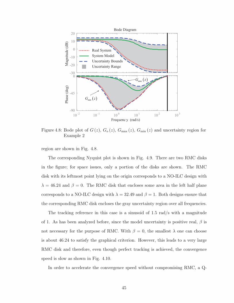
Mag

nit

ud

e (d

B)

-30

-20

-10

0

10

20

10-2

10-1

100

101

102

103

Ph

ase

(deg

)

-90

-45

0

Bode Diagram

Frequenc y (rad/s)

Uncertainty Bounds

System Model

Uncertainty Range

Real System

( )minG z

( )maxG z


region are shown in Fig. 4.8.

The corresponding Nyquist plot is shown in Fig. 4.9. There are two RMC disks

in the figure; for space issues, only a portion of the disks are shown. The RMC

disk with its leftmost point lying on the origin corresponds to a NO-ILC design with

λ = 46.24 and β = 0. The RMC disk that encloses some area in the left half plane

corresponds to a NO-ILC design with λ = 32.49 and β = 1. Both designs ensure that

the corresponding RMC disk encloses the gray uncertainty region over all frequencies.

The tracking reference in this case is a sinusoid of 1.5 rad/s with a magnitude

of 1. As has been analyzed before, since the model uncertainty is positive real, β is

not necessary for the purpose of RMC. With β = 0, the smallest λ one can choose

is about 46.24 to satisfy the graphical criterion. However, this leads to a very large

RMC disk and therefore, even though perfect tracking is achieved, the convergence

speed is slow as shown in Fig. 4.10.

In order to accelerate the convergence speed without compromising RMC, a Q-

45

0 0.5 1 1.5 2

Real Axis

-1.4

-1.2

-1

-0.8

-0.6

-0.4

-0.2

0

0.2

0.4

Imag

inar

y A

xis ( ),mine

U z

( )eU z

( ),maxeU z

RMC Disk for46.24, 0λ β= =

Uncertainty

Region

RMC Disk for32.49, 1λ β= =

Figure 4.9: RMC disks with two NO-ILC designs and uncertainty region at a fre-quency of 1.05 rad/s on the Nyquist plot for Example 2

filter can be introduced. With β > 0, λ can be smaller according to the expression of

radius 1/q and center 1/a of the RMC disk. Here, λ = 32.49 and β = 1 are picked as

an example. With this design, the algorithm converges faster, but at the expense of

a steady state tracking error as shown in Fig. 4.10. Note, as mentioned before, that

the monotonic convergence of ||ui − u∞||2 does not necessarily imply the monotonic

convergence of ||ei||2, especially in the presence of steady state error, which can be

seen in Fig. 4.10.

Hence, this example illustrates the utility of the developed NO-ILC design method

in adjusting the trade-off between convergence speed and steady state tracking error

while ensuring RMC.

The effect of noise is also explored in this example. For the same system model

and uncertainties, consider a scenario that a colored noise exists in the output mea-

surement channel. This colored noise is obtained by passing a white noise through a

46

Iteration Number

0 200 400 600 800 1000

2 N

orm

of

Tra

ckin

g E

rror

0

5

10

15

20

25

30

35

40

Iteration Number

0 200 400 600 800 1000

2 N

orm

of

Input

Dif

fere

nce

0

10

20

30

40

50

60

70

80

46.24, 0λ β= =

32.49, 1λ β= =

46.24, 0λ β= =

32.49, 1λ β= =

Figure 4.10: Tracking results of NO-ILC with λ = 46.24, β = 0 and λ = 32.49, β = 1in Example 2

high pass filter Wn(z) as shown in Eq. (4.16). The Fast Fourier Transform (FFT) of

this colored noise is shown in Fig. 4.11.

Wn(s) =s

s+ 100; W1(s) =

20

s+ 20(4.16)

In the following, three design options are considered to tolerate this noise. All

three designs use λ = 46.24 and β = 0 as the weighting parameters for NO-ILC.

Here, ei and em,i are used to denote the real tracking error and measured tracking

error (with noise) in the ith iteration.

Design Option 1 and Design Option 2 use the same Q-filter and learning gain

as the previous scenario where measurement noise does not exist. Design Option 1

simulates a scenario in which no action is taken towards the existing measurement

noise and the noisy tracking error, em,i, is directly used in the updating law:

ui+1 = Qui + Lem,i (4.17)

Design Option 2 simulates the case in which the noisy measured tracking error

47

0 50 100 150 200 250 300 350

Frequency (rad/s)

0

0.02

0.04

0.06

0.08

0.1

0.12

0.14

Mag

init

ud

e

FFT of Noise Signal

-60

-40

-20

0

20

Mag

nit

ud

e (d

B)

10 0 10 1 10 2 10 3

-180

-90

0

90

Ph

ase

(deg

)

Bode Diagram

Frequency (rad/s)

( )n

W z

1( )W z

Figure 4.11: FFT of the noise signal and Bode plot of W1(z) and Wn(z)

is filtered through a low-pass filter W1(s) as shown in Eq. (4.16) and the filtered

tracking error signal ef,i is used in the updating law:

ui+1 = Qui + Lef,i with Ef,i(s) = W1(s)Em,i(s) (4.18)

Design Option 3 uses a different Q-filter and learning gain compared with the two

previous designs. Given the fact that noise occurs in the output measurement at high

frequencies, the cost function is manipulated as follows:

Ji+1 (ui+1) = ‖ef,i+1‖22 + λ ‖ui+1 − ui‖2

2 + β ‖ui+1‖22 (4.19)

where ef,i+1 = W1em,i+1 with W1 representing the lifted matrix form of W1(z). Thus,

the same low-pass filter W1(z) is used as the one used in Design Option 2, but this

time the low-pass filter is incorporated into the cost function. The ILC updating law

48

0 200 400 600 800 1000

Iteration Number

0

5

10

15

20

25

30

35

40

2 N

orm

of

Tra

ckin

g E

rror

965 980 995

0.2

0.6

1

1.4

Option 1Option 2Option 3

0 5 10 15 20 25 30

Time (s)

-0.1

-0.08

-0.06

-0.04

-0.02

0

0.02

0.04

0.06

Tra

ckin

g E

rror

for

Las

t It

erat

ion

Figure 4.12: Tracking results of NO-ILC with λ = 46.24, β = 0 in Example 2 whenmeasurement noise exists

therefore becomes:

ui+1 = Qui + Lem,i

Q = (GTo WT

1 W1Go + λI + βI)−1(GTo WT

1 W1Go + λI)

L = (GTo WT

i W1Go + λI + βI)−1GTo WT

1

(4.20)

For the three design options, the 2 norm of the tracking errors in the iteration

domain are shown in Fig. 4.12. The tracking errors for the last iteration are also

shown in the right figure in Fig. 4.12.

By comparing the tracking results of Design Option 1 to the tracking results of

the scenario without measurement noise, in which case the tracking error converges

to zero as shown in Fig. 4.10, it is obvious that the measurement noise degrades the

system performance in the sense that it introduces some steady-state error. Both

Design Option 2 and 3 demonstrate improvements towards attenuating the effects

induced by noise, with a smaller steady state error achieved by Design Option 3.

49

-60

-40

-20

0

20

10-2

10-1

100

101

102

103

-180

-135

-90

-45

0

Uncertainty Bounds

System Model

Uncertainty Range

Real System

( )maxG z

( )minG z

Frequency (rad/s)

Phas

e (d

eg)

Mag

nit

ude

(dB

)

Bode Diagram


4.1.4.3 Example 3

This example illustrates a scenario in which the phase uncertainty at high fre-

quencies is larger than ± 90 degree. Consider the following system and modeling

error:

Go(s) =s+ 20

s+ 5; Ue(s) =

0.95

1.5s+ 1(4.21)

Let the upper and lower bounds of the model uncertainty be:

Ue,max(s) = 1.10.12s+ 1

0.1s+ 1; Ue,min(s) =

0.8

2.5s+ 1(4.22)

The Bode plot of the nominal model Go(z), real plant G(z) and the uncertainty

region are shown in Fig. 4.13.

The corresponding Nyquist plot is shown in Fig. 4.14. The two RMC disks

designed in the figure correspond to a NO-ILC design with λ = 0, β = 22.09 and

λ = 0, β = 30.25. Both designs ensure that the corresponding RMC disk encloses

50

-2 -1 0 1 2 3 4 5

Real Axis

-3

-2

-1

0

1

2

3

Imag

inar

y A

xis

30.25β =

Uncertainty

Region

( ),maxeU z( ),mineU z

( )eU z

RMC Disk for

RMC Disk for

22.09β =

Figure 4.14: RMC disks with two NO-ILC designs and uncertainty region at a fre-quency of 294.87 rad/s on the Nyquist plot for Example 3

the gray uncertainty region over all frequencies. In this case, λ can be picked as zero

since |Ue,max(ejθ)− 1| is smaller than 1 for all frequencies.

The tracking reference in this case is a sinusoid of 0.3 rad/s with a magnitude

of 0.1. Comparing the tracking results for the two designs as shown in Fig. 4.15,

it is confirmed that both designs guarantee RMC. Note that for robust monotonic

convergent NO-ILC design, usually the one with a larger β value leads to a larger

steady state error, which is demonstrated in this example. However, this is not always

true. The detailed analysis can be found in Chapter VI.

4.2 Frequency Dependent Weighting Matrices Design

In this section, instead of analyzing the robustness property of NO-ILC for a

diagonal weighting matrices design, a more general case is studied, i.e., non-diagonal

weighting matrices design. In this case, the weighting filters W1(z), W2(z) and W3(z)

are no longer constrained as constant gains. Furthermore, the graphical interpretation

51

0 2 4 6 8 102.4

2.6

2.8

3

3.2

3.4

3.6

3.8

4

0 2 4 6 8 100

0.05

0.1

0.15

0.2

0.25

0.3

0.35

0.4

2 N

orm

of

Tra

ckin

g E

rror

2 N

orm

of

Input

Dif

fere

nce

Iteration Number Iteration Number

0, 30.25λ β= =

0, 22.09λ β= =

0, 30.25λ β= =

0, 22.09λ β= =

Figure 4.15: Tracking results of NO-ILC with λ = 0, β = 22.09 and λ = 30, β = 30.25in Example 3

derived in Section 4.1, Eq. (4.10), is only a sufficient condition for the NO-ILC RMC

criterion, Eq. (3.2) whereas in this section, a graphical interpretation that is sufficient

and necessary for Eq. (3.2) is derived, which leads to RMC regions that can vary

over different frequencies. With this additional freedom in design, this new design

technique better addresses the fundamental trade-off of NO-ILC between robustness,

convergence speed and steady state error at difference frequencies, which is clarified

along with the discussion in Chapter V.

4.2.1 RMC Analysis

By plugging in G(z) = Ue(z)Go(z) into the RMC criterion, Eq. (3.2), the following

inequality can be obtained:

(L(ejθ)Go(e

jθ))2∣∣Ue(ejθ)∣∣2 +Q2(ejθ)− 1

− 2(Q(ejθ)L(ejθ)Go(e

jθ))

Re{Ue(ejθ)} < 0,∀θ ∈ [0, 2π] (4.23)

52

Note that both Q(ejθ) and L(ejθ)Go(ejθ) are real numbers and x(θ), y(θ) are defined

in Eq. (4.4). Then, Eq. (4.23) can be expressed as:

(x (θ)− c (θ))2 + y2 (θ) < r2 (θ) ,∀θ ∈ [0, 2π] (4.24)

where c (θ) and r (θ) are defined as:

c (θ)∆=

∣∣W1


(ejθ)∣∣2 +

∣∣W2

(ejθ)∣∣2

|W1 (ejθ)|2|Go (ejθ)|2

r (θ)∆=

∣∣W1


(ejθ)∣∣2 +

∣∣W2

(ejθ)∣∣2 +

∣∣W3

(ejθ)∣∣2

|W1 (ejθ)|2|Go (ejθ)|2

(4.25)

Note that Eq. (4.24) describes a disk, centered at c(θ) with a radius of r(θ). At

each frequency, as long as the possible Ue(ejθ) lies inside the disk enclosed by Eq.

(4.24), the NO-ILC updating law will have RMC against this modeling error. Note

that:

r (θ)− c (θ) =

∣∣W3

(ejθ)∣∣2

|W1 (ejθ)|2|Go (ejθ)|2(4.26)

If W3(ejθ) = 0, then r(θ) = c(θ), meaning the disk at this frequency θ cannot

cover any area of the left half of the complex plane, as shown in Fig. 4.16a. This

means that, at any frequency θ, as long as the real part of model uncertainty is

positive, i.e., Re{Ue(ejθ)} > 0, W3(ejθ) can be zero. This is an important insight

when designing NO-ILC since W3(ejθ) = 0 leads to zero steady state error at this

frequency, as discussed in later sections.

At any frequency θ, if the real part of model uncertainty is not positive, W3(ejθ)

cannot be zero if RMC is desired. If W3(ejθ) 6= 0, then r(θ) > c(θ), which means the

disk can cover some area in the left half plane as shown in Fig. 4.16b. This additional

coverage of the left half plane furnishes additional robustness, but at the expense of

a steady state error in the iteration domain, as discussed in Chapter V.

For a specific frequency, θ, the location and size of the RMC disk with respective

53

Re

Im

( )c θ

( )r θ

(a)

Re

Im

( )r θ

( )c θ

(b)

Figure 4.16: RMC region example for (a) W3(ejθ) = 0, and (b) W3(ejθ) 6= 0

to W1(ejθ), W2(ejθ) and W3(ejθ) are shown in Fig. 4.17:

1. When W2(ejθ) is held constant and W3(ejθ) = 0, increasing∣∣W1(ejθ)

∣∣ shifts the

center of the disk to the left and, at the same time, shrinks the disk. This is

shown in Fig. 4.17a.

2. When W1(ejθ) is held constant and W3(ejθ) = 0, increasing∣∣W2(ejθ)

∣∣ shifts the

center of the disk to the right and, at the same time, enlarges the disk. This is

shown in Fig. 4.17b.

3. Note that for both cases above, the disk does not enclose any region in the left

half plane. When W1(ejθ) and W2(ejθ) are held constant, increasing∣∣W3(ejθ)

∣∣increases the radius of the disk, keeping the disk center unchanged. Thus, the

disk can cover a certain area in the left half plane. This is shown in Fig. 4.17.c.

4.2.2 Design Guideline

Understanding the above analysis, a procedure for designing W1(z), W2(z) and

W3(z) can be laid out as follows:

1. Generate the upper and lower bound of the model uncertainty, Ue,max

(ejθ)

and

Ue,min

(ejθ), on the Bode plot as shown in Chapter III. Sample the frequency

54

Re

Im

( ) ( )

( ) ( )

( ) ( )

1 2

3 3

1 2

2 2

1 2

1 1

0j j

j j

j j

W e W e

W e W e

W e W e

θ θ

θ θ

θ θ

= =

=

<

( )1

1

jW e

θ( )2

1

jW e

θ

(a)

Re

Im

( ) ( )

( ) ( )

( ) ( )

1 2

3 3

1 2

2 2

1 2

1 1

0j j

j j

j j

W e W e

W e W e

W e W e

θ θ

θ θ

θ θ

= =

<

=

( )1

2

jW e

θ ( )2

2

jW e

θ

(b)

Re

Im

( ) ( )

( ) ( )

( ) ( )

1 2

3 3

1 2

2 2

1 2

1 1

j j

j j

j j

W e W e

W e W e

W e W e

θ θ

θ θ

θ θ

<

=

=

( )1

3

jW e

θ ( )2

3

jW e

θ

(c)

Figure 4.17: Illustration of how the RMC region changes with respect to W1(ejθ),W2(ejθ) and W3(ejθ)

range of the system using m ∈ N+ points {θ1, · · · , θm}. Ideally, m would be

infinity, but for practical purposes m can be picked sufficiently large. Transform

the uncertainty region onto the Nyquist plot at each frequency as shown in

Chapter III, θi for i ∈ [1,m].

2. For each frequency θi, design W1

(ejθi), W2

(ejθi)

and W3

(ejθi)

according to

Eq. (4.25) so that the RMC disk encloses the uncertainty region on the Nyquist

plot. To avoid a too conservative design, i.e., to avoid too slow convergence and

unnecessary steady state errors, the RMC disk should be as small as possible and

the leftmost point of the RMC disk should be as close to zero as possible. This

requires some tuning on the chosen W1 (z), W2 (z) and W3 (z) as is discussed

in the following bullet. Alternatively, the design of the weighting filters can

be formulated as an optimization problem to avoid manual tuning, as will be

addressed in Chapter VI.

3. For any frequency θi, set W3

(ejθi)

to zero if the uncertainty region lies in the

right half plane. If the disk needs to be enlarged towards the right hand side,

55

either increase W2

(ejθi)

or decrease W1

(ejθi)

. If the disk needs to be enlarged

to cover more area in the left half plane, increase W3

(ejθi).

As a comparison, with diagonal weightings in the cost function, i.e., Q = I,

R = λI and S = βI (or equivalently W1(z) = 1, W2(z) =√λ and W3(z) =

√β),

the degree of freedom for shaping the RMC region at different frequencies is very

limited. When W1(z), W2(z) and W3(z) are constant for all frequencies, a design

that is too conservative towards robustness over a certain frequency range is likely to

occur, which ultimately sacrifices the convergence speed and steady state error in this

frequency range as discussed in Chapter V. In contrast, this non-diagonal/frequency-

dependent filter design gives the opportunity to shape the RMC region at different

frequencies. This motivation for a frequency dependent weighting filter design will be

further obvious when the fundamental trade-off analysis at each frequency is presented

in the next chapter.

As a conclusion, the filters W1(z), W2(z) and W3(z) need to be designed so that

for every frequency, the possible modeling error, Ue(ejθ), which is unknown but lies

inside an uncertainty range, is guaranteed to lie inside the RMC region. For example,

considering the RMC design problem against the gray modeling uncertainty shown

in Fig. 4.18 at two specific frequencies ω1 and ω2, W1(z), W2(z), and W3(z) need

to be designed so that the gray uncertainty region lies inside the green RMC disk as

shown in Fig. 4.18. Note that Fig. 4.18 illustrates the design criterion for only two

frequencies. For the purpose of RMC against all possible modeling errors, Ue(z), it

must be ensured that the design criterion is valid for all frequencies.

Also note that, guaranteeing RMC against upper and lower bounds of the un-

certainty region on the Bode plot only does not necessarily guarantee RMC against

all the possible uncertainties. This can be seen in Fig. 4.18b since the disk would

be much smaller if it is designed only against the upper and lower bound at this

frequency as indicated by the two black dots on the solid curves. The reason is that

56

0 0.5 1 1.5

-0.6

-0.4

-0.2

0

0.2

0.4

0.6

Real Axis

Imag

inar

y A

xis

( ),maxeU z

( ),mineU z

( )1

,min

j

eU e

θ

( )1

,max

j

eU e

θ

Uncertantity

Region

RMC Disk

(a)

-1 0 1 2 3-3

-2.5

-2

-1.5

-1

-0.5

0

0.5

1

1.5

Imag

inar

y A

xis

Real Axis

4

( ),maxeU z

( ),mineU z Uncertantity

Region

RMC Disk

( )2

,min

j

eU e

θ

( )2

,max

j

eU e

θ

(b)

Figure 4.18: Achieving RMC for the example modeling uncertainty region: (a) at ω1

and (b) at ω2

the worst-case scenario on the Bode plot does not necessarily refer to the worst-case

scenario on the Nyquist plot.

4.2.3 Simulation Examples

In this section, two simulation examples are used to demonstrate the utility of

the developed frequency-dependent filter design approach. All the systems and filters

have the sampling time Ts = 0.001s and a total time steps N = 6000. The tracking

reference signal is a sinusoid at a frequency of 15 rad/s for the first example and is

a sinusoid at a frequency of 10 rad/s for the second example. These two examples

demonstrate the utility of the graphical design technique described in Section 4.2

for a robust monotonic convergent NO-ILC in the presence of model uncertainty.

Specifically, the first example deals with a positive real model uncertainty, a case in

which the Q-filter is not necessary for RMC and therefore perfect tracking can be

achieved. The second example deals with a non-positive real model uncertainty, a

case in which the Q-filter has to be used for RMC and thus some steady state error

is introduced. Note that for all the cases, the total time horizon length N = 6000 is

picked at least five times longer than the length of the non-zero impulse response of

57

Go(z), W1(z), W2(z), W3(z), thus the infinite time horizon analysis presented in this

thesis provides a good analysis and design tool.

4.2.3.1 Example 1

Consider a nominal plant, Go(z):

Go(z) =0.9975z

z − 0.995× 10−3 (4.27)

The Bode plot of the nominal plant is shown in Fig. 4.19 indicated as the solid

curve. Suppose there exists a positive real modeling error, which lies inside the range

shown as the gray region in Fig. 4.19. The upper and lower bounds of the model

uncertainty Ue,max(z) and Ue,min(z), shown as the dashed curve in Fig. 4.19, have the

following form:

Ue,max(z) =3z − 2.976

z − 0.9763; Ue,min(z) =

0.4z − 0.392

z − 0.99(4.28)

As Fig. 4.19 illustrates, the model is accurate at the low frequency range, whereas

the model accuracy starts to degrade at frequencies above 5 rad/s. Note that the

real system, G(z) = Ue(z)Go(z), can be any transfer function that lies inside the gray

region in Fig. 4.19. In this case, three example modeling errors are picked:

Ue,1(z) = Ue,max(z)

Ue,2(z) =2.25z2 − 4.438z + 2.188

z2 − 1.961z + 0.9618

Ue,3(z) =1.364z2 − 2.678z + 1.323

z2 − 1.966z + 0.9666

(4.29)

As discussed in Section 4.2.2, W3(z) is not needed for the purpose of RMC, because

the model uncertainty is positive real. This can be seen from the uncertainty range in

the Bode plot, since the phase difference between any uncertain plant and the system

58

Mag

nit

ud

e (d

B)

-80

-60

-40

-20

0

10-1

100

101

102

103

104

Ph

ase

(deg

)

-135

-90

-45

0

Frequenc y (rad/s)

System Uncertainty Upper Bound

System Model


model never exceeds ±90 degrees. W2(z) should be designed as a low pass filter, since

the model uncertainty is large at higher frequencies. Following the design guidelines

in Section 4.2.2, the filters are designed as W1(z) = 1, W3(z) = 0 and

W2(z) =0.02z − 0.01901

z − 0.9802(4.30)

so that the possible uncertainty region lies inside the RMC disk at all frequencies. As

an example, the disk plots at two frequencies, one above and one below the reference

frequency, are shown in Fig. 4.20. Fig. 4.20a is for ω = 3.72 rad/s and Fig. 4.20b is

at ω = 16.63 rad/s. The black dots indicate the values of Ue,max(ejθ) and Ue,min(ejθ)

on the complex plane at the corresponding frequencies. The gray region in Fig.

4.20 indicates the model uncertainty range, which corresponds to the gray region in

Fig. 4.19 at this specific frequency. In both frequencies shown, the RMC criterion

is satisfied, since the green disk includes the gray region. The same holds for all

frequencies. Therefore, for all the possible modeling errors, the designed NO-ILC

59

Real Axis

Imag

inar

y A

xis

Real Axis

Imag

inar

y A

xis

-0.5 0 0.5 1 1.5 2 2.5 3 3.5

-1.5

-1

-0.5

0

0.5

1

1.5

-0.5 0 0.5 1 1.5 2 2.5 3 3.5

-1.5

-1

-0.5

0

0.5

1

1.5

( )a ( )b

( ),mineU z

( ),min

j

eU e θ

RMC

Disk

( ),maxUe z( ),maxU j

e e θ

Uncertainty

Region

RMC

Disk( ),maxUe z( ),maxU j

e e θ

Uncertainty

Region( ),mineU z

( ),min

j

eU e θ

Figure 4.20: RMC disks for Example 1 at different frequencies: (a) 3.72 rad/s (b)16.63 rad/s

algorithm will be robust monotonic convergent.

With this filter design, the tracking error in the iteration domain is shown in Fig.

4.21. Remember that the tracking error and input difference are defined as following:

Tracking Error∆= yd − yi

Input Difference∆= ui − u∞

(4.31)

As shown in Fig. 4.21, both the tracking error and input difference are monotonically

decreasing as the iteration number increases.

4.2.3.2 Example 2

In this example, the following nominal plant, Go(z), is used:

Go(z) =0.398z2 + 0.96z

z2 − 1.995z + 0.995× 10−3 (4.32)

Similar to the previous example, the Bode plots of the nominal plant and uncer-

tainty range are shown in Fig. 4.22. The lower bound of model uncertainty, Ue,min(z),

60

2 N

orm

of

Tra

ckin

g E

rror

Iteration Number

2 N

orm

of

Input

Dif

fere

nce

Iteration Number

0 5 10 15 20 25 300

5

10

15

20

25

30

35

40

0 5 10 15 20 25 300

100

200

300

400

500

600

( ),1Modeling Error:e

U z


U z


U z


U z


U z


U z

Figure 4.21: Monotonic convergence of tracking error and input difference in the it-eration domain for Example 1

in this case has the following form:

Ue,min(z) =1.178z − 0.7854

z2 − 1.96z + 0.9608× 10−3 (4.33)

The upper bound of the model uncertainty is Ue,max(z) = 1. Three example

modeling errors are picked:

Ue,1(z) = Ue,min(z)

Ue,2(z) =(4.573z2 − 7.492z + 2.964)× 10−3

z3 − 2.847z2 + 2.699z − 0.8521

Ue,3(z) =1.111z2 − 1.655z + 0.5879

z2 − 1.96z + 0.9608× 10−2

(4.34)

In this case, W3(z) is not needed for the low frequencies, because all the possible

modeling errors are in the right half plane at low frequencies. However, W3(z) is

needed at high frequencies, since some component of the possible modeling error lies

in the left half plane at high frequencies. Following the design guidelines in Section

61

−200

−150

−100

−50

0

50

Mag

nit

ude

(dB

)

100

101

102

103

104

−450

−360

−270

−180

−90

0

Phas

e (d

eg)

Frequency (rad/s)

System Uncertainty Lower Bound

System Model


4.2.2, the filters are designed as W1(z) = 1, W2(z) = 0.1 and

W3(z) = 10−3 × 0.4137z2 + 0.8274z3 + 0.0122z2 + 0.803z − 0.4015

z5 − 4.94z4z + 9.761z3 − 9.644z2 + 4.765z − 0.9418(4.35)

so that the possible modeling error lies inside the RMC disk for all frequencies.

The RMC disk plots at two example frequencies are shown in Fig. 4.23. Fig.

4.23a is at 7.90 rad/s and Fig. 4.23b is at 31.51 rad/s.

The tracking error and input difference in the iteration domain are shown in Fig.

4.24. Since the value of∣∣W3(ejθ)

∣∣ is non-zero at 10 rad/s, which is the frequency of

tracking reference signal, a steady state tracking error is expected. Also note that

the 2-norm of the input difference is decreasing monotonically, confirming that the

design has RMC against the given uncertainty range.

62

Imag

inar

y A

xis

Imag

inar

y A

xis

Real Axis

( )aReal Axis

( )b

-1 -0.5 0 0.5 1 1.5 2 2.5 3

-1.5

-1

-0.5

0

0.5

1

1.5

-1 -0.5 0 0.5 1 1.5 2 2.5 3

-1.5

-1

-0.5

0

0.5

1

1.5

RMC

Disk

Uncertainty

Region

( ),mineU z( ),min

j

eU e θ

Uncertainty

Region

RMC

Disk

( ),mineU z

( ),min

j

eU e θ

Figure 4.23: RMC disk for Example 2 at different frequencies: (a) 7.90 rad/s (b)31.51 rad/s

2 N

orm

of

Tra

ckin

g E

rror

Iteration Number0 5 10 15 20 25 30

0

5

10

15

20

25

30

35

40


U z


U z


U z

2 N

orm

of

Input

Dif

fere

nce

Iteration Number0 5 10 15 20 25 30

90

100

110

120

130

140

150

160


U z


U z


U z

Figure 4.24: Tracking error and input difference in iteration domain for Example 2

63

4.3 Conclusion

Using the new model uncertainty formulation presented in Chapter III, which

incorporates additional phase information compared with the traditional one, a fre-

quency domain analysis on the RMC of NO-ILC has been developed to explain the

relationships between RMC against the modeling errors and the NO-ILC weighting

filters.

The first section of this chapter derives a sufficient condition for the RMC cri-

terion for scalar NO-ILC wighting filters, which leads to a graphical characterization

of the allowable modeling error on the Nyquist plot. The relationship between the

RMC region and the scalar weighting filters is analyzed. The analysis points out how

the RMC region changes with respect to different NO-ILC weighting parameters λ

and β. Therefore, this tool can be used as a frequency domain design method for

robust monotonic convergent NO-ILC against model uncertainties. Three simula-

tion examples are presented to demonstrate the effectiveness of the proposed design

method.

The second section extends the analysis in the previous section in two aspects.

First, a necessary and sufficient condition is derived for the RMC criterion for

NO-ILC. Second, the scalar weighting filter design is extended to general LTI weight-

ing filter designs. The RMC region is also interpreted on Nyquist plot and the rela-

tionship between the RMC region and weighting filters is analytically characterized.

The analysis leads to a more aggressive design technique, which better addresses the

trade-off between robustness, convergence speed and steady state error at different

frequencies that is discussed in the next chapter.

64

CHAPTER V

Fundamental Trade-off of NO-ILC and Its

Optimality

The discussions in the previous chapter focus on design methodologies for RMC

against model uncertainty. However, robustness is not the only concern when design-

ing NO-ILC. Besides robustness, convergence speed and steady state error are also

important performance criterion. A good NO-ILC design should have just enough

robustness against the model uncertainty and, at the same time, maximize the con-

vergence speed and minimize the steady state error. Therefore, it is important to

understand the trade-off between robustness, convergence speed and steady state er-

ror for NO-ILC. In the literature, some qualitative statements about this trade-off

already exist. In this chapter, through the frequency domain analysis, a quantitative

characterization of this trade-off is presented for the first time.

Given the fact that NO-ILC is subject to this fundamental trade-off, it is inter-

esting to ask whether other LTI ILC updating laws can bypass this trade-off. It is

demonstrated that the answer is no. In another word, NO-ILC is the optimal solu-

tion in terms of addressing the trade-off between robustness, convergence speed and

steady state error among LTI ILC updating laws. The proof of this optimality is

presented in the second half of this chapter.

65

5.1 Fundamental Trade-off Between Robustness, Convergence

Speed and Steady State Error

Against any modeling error, Ue(z), diagonal weightings can be used in the cost

function to ensure RMC for NO-ILC; i.e., Q = I, R = λI and S = βI, which

corresponds to W1(z) = 1, W2(z) =√λ and W3(z) =

√β. However, robustness is not

the only concern, since convergence speed and steady state error are also important

factors. A fundamental trade-off exists between robustness, convergence speed and

steady state error, and using frequency dependent weightings in the cost function

helps better address this trade-off. This section shows the analytical relationship

among these three performance criteria at each frequency for any robust monotonic

convergent NO-ILC using the cost function, Eq. (1.1).

To this end, the robustness, convergence speed and steady state tracking error for

NO-ILC are first defined at each frequency.

5.1.1 Robustness

Robustness is defined as the allowable modeling error for a specific NO-ILC design.

In this work, RMC region is used to quantify the robustness of NO-ILC. As discussed

in the previous chapter, the RMC region at each frequency is a disk. Hence, the

radius of this disk is used in this work to characterize the robustness. Larger disk

radius corresponds to larger robustness. Thus, at each frequency, robustness, denoted

as RB(θ) here, is defined as the following:

RB (θ) , r (θ) =

∣∣W1


(ejθ)∣∣2 +

∣∣W2

(ejθ)∣∣2 +

∣∣W3

(ejθ)∣∣2

|W1 (ejθ)|2|Go (ejθ)|2(5.1)

Note that the robustness, RB(θ), is a number that lies in the interval [1,∞). This

is consistent with the fact that the radius of the RMC disk for NO-ILC is guaranteed

to be larger than one, because when W2(z) = W3(z) = 0, NO-ILC is the same as

66

plant inversion and the RMC disk radius in this case is one (Harte et al., 2005).

5.1.2 Convergence Speed

Convergence speed denotes how fast the input sequence converges. Before giving

the definition of convergence speed, the concept of convergence ratio is first intro-

duced. Convergence ratio, CR(θ), is a ratio defined as:

CR (θ) ,

∣∣∣∣∣ui+1

(ejθ)− u∞

(ejθ)

ui (ejθ)− u∞ (ejθ)

∣∣∣∣∣ (5.2)

where u∞(z) denotes the input sequence when ILC converges. From the frequency

domain updating law, Eq. (2.15), and considering the nominal performance, i.e.,

there is no model uncertainty, the following equation can be derived:

ui+1(z)− u∞(z) = (Q(z)− L(z)Go(z)) (ui+1(z)− u∞(z)) (5.3)

Therefore, the convergence ratio becomes:

CR(θ) =∣∣Q(ejθ)− L(ejθ)Go(e

jθ)∣∣

=

∣∣W2

(ejθ)∣∣2

|W1 (ejθ)|2|Go (ejθ)|2 + |W2 (ejθ)|2 + |W3 (ejθ)|2(5.4)

Note that the convergence ratio, CR(θ), is a number in the interval [0, 1). CR(θ) =

1 means the input sequence is not converging, while CR(θ) = 0 means the input

sequence converges infinitely fast, like a dead-beat control in the iteration domain.

The convergence speed, CS(θ), is then defined as:

CS(θ) , 1− CR(θ)

=

∣∣W1


(ejθ)∣∣2 +

∣∣W3

(ejθ)∣∣2

|W1 (ejθ)|2|Go (ejθ)|2 + |W2 (ejθ)|2 + |W3 (ejθ)|2(5.5)

67

Thus, convergence speed, CS(θ), is also a number that lies in the interval (0, 1].

CS(θ) = 0 means the input sequence is not converging, whereas CS(θ) = 1 means the

input sequence is converging infinitely fast.

Note that the definition of convergence speed, Eq. (5.5), is for steady state signals.

Transient signals always exist and the worst-case convergence ratio in terms of the 2-

norm of the input sequence is |Q(z)−L(z)Go(z)|∞ according to Parseval’s Theorem,

which has been widely used in the ILC literature to characterize the convergence

speed. However, |Q(z) − L(z)Go(z)|∞ does not provide any information about the

frequency components. In many cases, this leads to a conservative estimation of the

convergence speed.

5.1.3 Steady State Error

It is well-known in the literature that even if the nominal performance of NO-ILC

converges, a steady state error exists if Q(z) 6= 1. In this paper, the steady state

error, SSE(θ), for each frequency, θ, is defined as:

SSE(θ) ,

∣∣∣∣∣ud(ejθ)− u∞

(ejθ)

ud (ejθ)

∣∣∣∣∣ (5.6)

where ud(z) denotes the ideal input that achieves perfect tracking. Note that ud(z) is

unknown in general. However, from the frequency domain updating law, Eq. (2.15),

one can obtain the following equation:

SSE(θ) =

∣∣W3

(ejθ)∣∣2

|W1 (ejθ)|2|Go (ejθ)|2 + |W3 (ejθ)|2(5.7)

Note that the steady state error is a number in the interval [0, 1]. SSE(θ) = 0

means the input converges to the ideal one at this frequency, while SSE(θ) = 1 means

the input signal is zero. Also note that when W3(ejθ) = 0, SSE(θ) = 0, which is

consistent with the fact that there will be no steady state error if Q-filter is not used;

68

i.e., Q(z) = 1.

5.1.4 Expressing the Fundamental Trade-off for NO-ILC

In the previous sections, mathematical expressions for robustness RB(θ), conver-

gence speed CS(θ) and steady state error SSE(θ) at each frequency have been defined.

In this section, the relationship between these three terms is analytically expressed.

This relationship is a fundamental trade-off for the nominal performance of NO-ILC.

From Eq. (5.1), (5.5) and (5.7), it can be shown that the robustness, convergence

speed and steady state error at each frequency for NO-ILC satisfy the following

relationship:

1

CS(θ)RB(θ)+ SSE(θ) = 1 (5.8)

The significance of the above equation is that it quantitatively describes the trade-

off between robustness, convergence speed and steady state error of NO-ILC at each

frequency. This equation is analogous to the fundamental trade-off S(θ)+T (θ) = 1 in

feedback control, where S(θ) is the sensitivity function and T (θ) is the complementary

sensitivity function at each frequency θ. The design of NO-ILC is a design of balancing

the abovementioned trade-off.

For a NO-ILC design with W3(ejθ) = 0, SSE(θ) is zero, and the robustness and

convergence speed have an inverse relationship as shown by the solid curve in the

Fig. 5.1a. Note that, as discussed earlier, NO-ILC in this case guarantees a minimum

robustness of 1. As W3(ejθ) increases, SSE(θ) increases, which shifts the curve up, as

shown by the dashed curve in Fig. 5.1a.

For a NO-ILC design with W2(ejθ) = 0, CS(θ) is one according to Eq. (5.5). From

Eq. (5.8), it follows that RB(θ) = 1/(1− SSE(θ)) as shown by the solid curve in the

Fig. 5.1b. As W2(ejθ) increases, CS(θ) decreases, which shifts the curve up, as shown

by the dashed curve in Fig. 5.1b.

For the purpose of better visualizing the fundamental trade-off of NO-ILC char-

69

11

()

Robustness,RBθ

0 ( )Convergence Speed,CS θ

( ) 0SSE θ =

( ) 0SSE θ >

(a)

( )Steady State Tracking Error,SSE θ

11

0

()

Robustness,RBθ ( ) 1CS θ =

( ) 1CS θ <

(b)

Figure 5.1: Illustration of the trade-off between (a) convergence speed and robustness,and (b) steady state error and robustness

acterized by Eq. (5.8), a 3D Pareto plot of the three performance metrics of NO-ILC

is shown in Fig. 5.2. At each frequency, robustness, convergence speed and steady

state error lie on the Pareto surface. Note that the most aggressive NO-ILC (plant

inversion), i.e., W2(ejθ) = W3(ejθ) = 0, is at the point of the surface with SSE(θ) = 0,

CS(θ) = 1 and RB(θ) = 1.

This fundamental trade-off analysis can be used in the NO-ILC to design for

optimal performance at each frequency according to various robustness, convergence

speed and steady state error requirements.

5.1.5 Simulation Example

In this example, the nominal performance of NO-ILC is analyzed. The perfor-

mance of NO-ILC is compared between using the proposed frequency-dependent filter

design method, , as discussed in Section 4.2, and using diagonal weighting matrices,

as discussed in Section 4.1. Eq. (5.8) shows that robustness, convergence speed

and steady state error cannot be improved at the same time at a given frequency.

Therefore, the design of NO-ILC needs to balance the trade-off between the above-

mentioned quantities according to different requirements at different frequencies. This

70

SteadyState

Tracking

Error,

()

SSEθ

Converg

ence Sp

eed,( )CSθ

0

()

Robustness,RBθ

Figure 5.2: Performance surface for NO-ILC

example is built on the scenario that the diagonal weighting matrix design is required

to meet at least the robustness that has been achieved by using the proposed filter

design. The results show that either convergence speed or steady state error comes

as a sacrifice when diagonal weighting matrices are used. All the systems and filters

have the sampling time Ts = 0.001s and a total time steps N = 6000, which is at least

five times longer than the length of the non-zero impulse response of Go(z), W1(z),

W2(z), W3(z), thus the infinite time horizon analysis presented in this paper provides

a good analysis and design tool.

Two nominal plants are used in this section:

Go,Ex1(z) =0.9975z

z − 0.995× 10−3

Go,Ex2(z) =0.398z2 + 0.396z

z2 − 1.995z + 0.995× 10−3

(5.9)

Consider the first nominal plant in Eq. (5.9), Go,Ex1(z). In Section 4.2.3.1, a

71

10-2

10-1

100

101

102

103

0

0.1

0.2

0.3

0.4

0.5

0.6

0.7

0.8

0.9

1

()

1RBθ

1 rad/sω =25 rad/sω =

Frequency (rad/s)

( ) ( )2 2,2W z W z=

( ) ( )2 2,1W z W z=

(a)

0 2 4 6 8 100

5

10

15

20

25

30

35

40

Iteration Number

2NormofTrackingError ( ) ( )2 2,1 ; 25 rad/sW z W z ω= =

( ) ( )2 2,1 ; 1 rad/sW z W z ω= =

( ) ( )2 2,2 ; 25 rad/sW z W z ω= =

( ) ( )2 2,2 ; 1 rad/sW z W z ω= =

(b)

Figure 5.3: (a) Robustness at different frequency for W2,1(z) and W2,2(z) and (b) 2norm of tracking error in iteration domain

NO-ILC filter design has been proposed with:

W1(z) = 1

W2,1(z) =0.02z − 0.01901

z − 0.9802

W3(z) = 0

(5.10)

for the nominal plant Go,Ex1(z). Let W1(z) and W3(z) be the same but use W2(z) =

W2,2(z) =√λ to guarantee that its robustness at each frequency is no smaller com-

pared with the previous design. As discussed in the previous section, the robustness

at each frequency, RB (θ), is characterized using Eq. (5.1). The smallest value of√λ

in this case is 0.5, which is the DC gain of W2,1(z). The robustness, RB (θ), with

respect to different frequencies for the two designs is shown in Fig. 5.3a.

In this case, since W3(z) = 0, which means there will be no steady state error,

the results show how the robustness and convergence speed are related at different

frequencies with different W2(z) designs. At 1 rad/s, using W2(z) = W2,1(z) and

W2(z) = W2,2(z) gives the same robustness as shown in Fig. 5.3a. The convergence

speed of these two different designs is almost the same at this specific frequency as

shown in Fig. 5.3b, since the thin solid line and the thick solid line overlap with

72

each other. At the frequency of 25 rad/s, the robustness with W2(z) = W2,2(z) is

larger compared with the robustness of the design with W2(z) = W2,1(z) as shown in

Fig. 5.3a. According to the fundamental trade-off analysis in the previous section,

larger robustness at this frequency corresponds to slower convergence speed. This

is consistent with the results shown in Fig. 5.3b, since the thin dashed line (with a

design of W2(z) = W2,2(z)) converges slower than the thick dashed line (with a design

of W2(z) = W2,1(z)).

The relationship between robustness and convergence speed can also be evaluated

quantitatively according to Eq. (5.8) for this example, since the steady state error is

zero. At the frequency of 1 rad/s, (RB(θ))−1 for both designs is 0.939 as shown in

Fig. 5.3a. According to Eq. (5.8), a convergence speed of 0.939 is expected, which

corresponds to a convergence ratio of 0.061. From Fig. 5.3b, the actual converge

ratio is roughly 0.060, confirming the analysis. Similarly, at the frequency of 25 rad/s,

(RB(θ))−1 is 0.383 for W2,2(z) and is 0.560 for W2,1(z). The expected corresponding

convergence ratios are 0.617 and 0.440, respectively. The actual convergence ratios

can be calculated according to the thin and thick dashed line shown in Fig. 5.3b,

which is roughly 0.612 for W2,2(z) and is 0.447 for W2,1(z). This agreement between

the theoretical and actual values demonstrates the utility of Eq. (5.8). The minor

differences between the theoretical and actual numbers are due to the fact that the

frequency domain analysis is for an infinite time horizon, but the simulations are run

for a finite time.

Consider the second nominal plant in Eq. (5.9), Go,Ex2(z). In Section 4.2.3.2, a

NO-ILC filter design has been proposed with:

W1(z) = 1

W2(z) = 0.1

W3,1(z) = 10−3 × 0.4137z2 + 0.8274z3 + 0.0122z2 + 0.803z − 0.4015

z5 − 4.94z4z + 9.761z3 − 9.644z2 + 4.765z − 0.9418

(5.11)

73

10-2

10-1

100

101

102

103

0

0.1

0.2

0.3

0.4

0.5

0.6

0.7

0.8

0.9

1

27.48 rad/sω =

10 rad/sω =

()

1RBθ

Frequency (rad/s)

( ) ( )3 3,2WW z z=

( ) ( )3 3,1WW z z=

(a)

0 2 4 6 8 100

10

20

30

40

50

60

Iteration Number

2NormofTrackingError ( ) ( )3 3,1 ; 10 rad/sW z W z ω= =

( ) ( )3 3,1 ; 27.48 rad/sW z W z ω= =

( ) ( )3 3,2 ; 10 rad/sW z W z ω= =

( ) ( )3 3,2 ; 27.48 rad/sW z W z ω= =

(b)

Figure 5.4: (a) Robustness at different frequencies for W3,1(z) and W3,2(z) and (b) 2norm of tracking error in iteration domain

for nominal plant Go,Ex2(z). Let W1(z) and W2(z) be the same, but use W3(z) =

W3,2(z) =√β to guarantee that its robustness at each frequency is no smaller com-

pared with the previous design. The smallest value of√β in this case is 1.44. The

robustness, RB (θ), with respect to different frequencies for the two designs is shown

in Fig. 5.4a.

In this case, since W2(z) = 0.1 is quite small compared with W3(z) and Go,Ex2(z),

which means the learning will be very fast, the results can be studied to see how the

robustness and steady state error are related at different frequencies with different

W3(z) designs. At 27.8 rad/s, using W3(z) = W3,1(z) and W3(z) = W3,2(z) gives

the same robustness as shown in Fig. 5.4a. The steady state errors of these two

different designs are very close at this specific frequency as shown in Fig. 5.4b. At

frequency of 10 rad/s, the robustness with W3(z) = W3,1(z) is larger compared with

the robustness of the design with W3(z) = W3,2(z) as shown in Fig. 5.4a. According

to the fundamental trade-off analysis in the previous section, larger robustness at this

frequency corresponds to a larger steady state error. This is consistent with the results

shown in Fig. 5.4b, since the thin dashed line (with a design of W3(z) = W3,2(z))

converges to a larger steady state error than the thick dashed line (with a design of

74

W3(z) = W3,1(z)).

The relationship between robustness and steady state error can be quantitatively

investigated based on these simulation results since CS(θ) ≈ 1 in this scenario. At the

frequency of 27.48 rad/s, (RB(θ))−1 for both designs is 0.642 as shown in Fig. 5.4a.

According to Eq. (5.8), a steady state error of 0.358 is expected. From Fig. 5.4b,

the actual steady state error is 0.356 for W3,1(z) and 0.372 for W3,2(z). Similarly, at

the frequency of 10 rad/s, (RB(θ))−1 is 0.934 for W3,1(z) and 0.375 for W3,2(z). The

expected steady state errors are 0.066 and 0.625, respectively. The actual steady state

errors are roughly 0.061 for W3,1(z) and 0.624 for W3,2(z). This agreement between

the theoretical and actual values illustrates the utility of Eq. (5.8).

Fig. 5.4 shows that the learning speed for all cases is very fast because W2(z) is

small and this is consistent with Eq. (5.5). Also note that, theoretically, the steady

state error in the iteration domain for this case at frequency of 27.48 rad/s should

be the same for an infinite time horizon. Note that the frequency domain analysis

for NO-ILC is for infinite time horizon, whereas NO-ILC is always implemented in

finite time horizon in the time domain. The small difference between the red solid

line and the blue solid line in Fig. 5.4b is due to the transients in the time domain.

Since W3(z) used is different, this leads to different transients in the time domain.

Fig. 5.5 shows the error signal in the time domain for both designs at the 10th

iteration. Notice that the transients occur at both the beginning and ending due to

the zero-phase filter nature of NO-ILC. In this case, the transients with the design of

W3(z) = W3,1(z) are smaller than the transients with the design of W3(z) = W3,2(z).

Therefore, a smaller steady state error in the iteration domain is expected with the

design of W3(z) = W3,1(z) as shown in Fig. 5.4b.

In conclusion, for the nominal performance, using the proposed frequency-dependent

filter design in NO-ILC can lead to more degrees of freedom to design the NO-ILC

performance, i.e., robustness, convergence speed and steady state error, at different

75

0 1 2 3 4 5 6-0.6

-0.4

-0.2

0

0.2

0.4

0.6

0.8

Transients

Time (s)

TrackingError

( ) ( )3 3,2W z W z=

( ) ( )3 3,1W z W z=

Figure 5.5: Comparison of the tracking error for Go,Ex2 with different W3(z) designsat 27.48 rad/s after 10th iteration

frequencies compared with NO-ILC design with constant weighting matrices.

5.2 Optimality of NO-ILC

The previous section quantitatively presents the fundamental trade-off between

robustness, convergence speed and steady state error at each frequency for NO-ILC

for Single-Input-Single-Output (SISO) system. An interesting question that naturally

follows is whether this fundamental trade-off also exists for general LTI ILC updating

laws:

ui+1(z) = Q(z)ui(z) + L(z)ei(z) (5.12)

In this section, it is shown that, for general LTI ILC updating laws, there exists

some quantifiable relationship between the three performance indices at each fre-

quency. Furthermore, in the scope of LTI ILC updating laws, NO-ILC is the optimal

solution in terms of balancing the trade-off between these three performance indexes

over all the frequencies.

In this section, first, the results will be presented in a case where the Q-filter is

76

disabled in the updating law Eq. (5.12). Then, the results will be generalized to the

scenarios where the Q-filter is used.

5.2.1 Without Q-Filter

In this section, the following LTI ILC updating law will be considered:

ui+1(z) = ui(z) + L(z)ei(z) (5.13)

Since the Q-filter is disabled in this scenario, there will be no steady state error

if the ILC converges. In the following two sections, the question of how much model

uncertainty can be tolerated will be explored and then the relationship between the

robustness and convergence speed will be addressed.

5.2.1.1 How Much Uncertainty Can Be Tolerated?

In this section, the research question of how much model uncertainty can be

tolerated will be answered. Plugging Q(z) = 1 into the RMC criterion Eq. (3.2), the

following can be obtained:

∣∣1− Ue (ejθ)Go

(ejθ)L(ejθ)∣∣ < 1, ∀θ ∈ [0, 2π] (5.14)

Let the complex numbers, Go

(ejθ)L(ejθ)

and Ue(ejθ), be:

Ue(ejθ), x(θ) + jy(θ)

Go

(ejθ)L(ejθ), m(θ) + jn(θ)

(5.15)

where x(θ), m(θ) and y(θ), n(θ) denote the real and complex parts of Ue(ejθ)

and

Go

(ejθ)L(ejθ)

respectively. Substituting the above equations into Eq. (5.14) gives

77

the following:

(x(θ)− cx(θ))2 + (y(θ)− cy(θ))2 < r(θ), ∀θ ∈ [0, 2π) (5.16)

where (cx(θ), cy(θ)) and r(θ) denote the center and radius of a disk. They are functions

of m(θ) and n(θ) as shown in the following:

cx(θ) =m(θ)

m2(θ) + n2(θ)

cy(θ) = − n(θ)

m2(θ) + n2(θ)

r(θ) =1√

m2(θ) + n2(θ)

(5.17)

Thus, the allowable model uncertainty can be characterized with a disk centered

at (cx(θ), cy(θ)) with a radius of r(θ) at each frequency θ. As an example shown

in Fig. 5.6 at a particular frequency θo, the disk is illustrated as the light green

region. As long as the model uncertainty Ue(z) lies inside the green disk over all the

frequencies, RMC is achieved. The vector Go

(ejθo)L(ejθo)

is also illustrated using

the red arrow in Fig. 5.6, which is further discussed in the next section.

5.2.1.2 Relationship Between Robustness and Convergence Speed

For the scenario when the Q-filter is disabled, there will not be any steady state

error if the ILC converges, which has been well understood in the literature. There-

fore, in this section, the relationship between the robustness and convergence speed

will be investigated. First, the definitions of robustness and convergence speed will

be introduced.

The radius of the disk that describes the allowable modeling uncertainties is used

here to characterize the robustness. The definition of the robustness over different

78

Allowable Model Uncertainty

( ) ( )o oj j

oG e eθ θL

( ) ( )( ),o om nθ θ

( ) ( )1 o o

o

j jG e e

θ θ− L

( )1,0

( ) ( )( ),x o y oc cθ θ

( )or θ

Figure 5.6: Illustration of allowable model uncertainties and the vectorGo

(ejθo)L(ejθo)

on the complex plane at a particular frequencyθo

frequencies, RB (θ), is shown as following:

RB (θ) , r (θ) =1

|Go (ejθ)L (ejθ)|∈

(√2

2,∞

)(5.18)

As can be seen here, a too large learning gain L (θ) potentially leads to a very small

robustness since, according to its definition, RB(θ) =∣∣Go

(ejθ)L(ejθ)∣∣−1

. Comparing

this to NO-ILC, note that NO-ILC guarantees a minimum robustness of 1 over all

the frequencies.

For a robust monotonic convergent ILC updating law, the convergence ratio CR (θ)

at each frequency θ is defined as following:

CR (θ) ,∣∣1−Go

(ejθ)L(ejθ)∣∣ ∈ [0, 1) (5.19)

where CR (θ) = 1 means the ILC is not converging and CR (θ) = 0 means the ILC

79

converges rapidly. The definition of convergence speed CS (θ) follows immediately:

CS (θ) , 1− CR (θ) ∈ (0, 1] (5.20)

where CS (θ) = 1 means the ILC converges rapidly and CS (θ) = 0 means the ILC does

not converge. The following proposition then characterizes the relationship between

robustness and convergence speed at each frequency θ.

Proposition V.1. For a monotonic convergent ILC updating law Eq. (5.13), its

robustness and converge speed satisfy the following relationship:

1

RB (θ) CS (θ)≥ 1, ∀θ ∈ [0, 2π] (5.21)


Note that the relationship between robustness and convergence speed for NO-ILC

when the Q-filter is disabled has been previously reported in the previous section:

1

RB (θ)CS (θ)= 1, ∀θ ∈ [0, 2π] (5.22)

To this end, the optimality of NO-ILC when the Q-filter is disabled in terms of the

trade-off between robustness and convergence speed at each frequency is illustrated

in Fig. 5.7. The red curve denotes the Pareto curve for NO-ILC while the gray region

indicates the landing point for LTI ILC updating law Eq. (5.13). This demonstrates

the optimality of NO-ILC in terms of balancing the trade-off between robustness

and convergence speed at each frequency. It is worth mentioning here though that

the performance index of the ILC updating law Eq. (5.13) could potentially lie on

the the Pareto curve for certain frequencies but NO-ILC guarantees this for all the

frequencies.

80

1

1

0 ( )Convergence Speed, CS θ

()

Robust

nes

s,R

Bθ

Pareto Curve for NO-ILC

Performance Index Region

for General ILC, Eq. (6)

Figure 5.7: Trade-off between robustness and convergence speed for general LTI ILCupdating laws when Q-filter is disabled

5.2.2 With Q-Filter

In this section, the results derived in the previous sections are extended for the

general case when Q-filter is used in the ILC updating law. Similar to the previous

section, the region for the allowable model uncertainty is addressed first followed by

the derivation of the relationship between robustness, convergence speed and steady

state error.

5.2.2.1 How Much Uncertainty Can Be Tolerated?

Following the similar ideas presented in the previous section, the allowable model

uncertainty analysis is extended to a scenario where the Q-filter is used.

The frequency domain RMC criterion Eq. (3.2) can be re-written as:

∣∣Q (ejθ)− Ue (ejθ)Go

(ejθ)L(ejθ)∣∣ < 1, ∀θ ∈ [0, 2π] (5.23)

Define the complex number Q(ejθ)

as:

Q(ejθ), p(θ) + jq(θ) (5.24)

81

Pluging Eq. (5.15) and Eq. (5.24) into Eq. (5.23) gives Eq. (5.16) but with cx(θ),

cy(θ) and r(θ) equal to the followings:

cx(θ) =m(θ)p(θ) + n(θ)q(θ)

m2(θ) + n2(θ)

cy(θ) = −n(θ)p(θ)−m(θ)q(θ)

m2(θ) + n2(θ)

r(θ) =1√

m2(θ) + n2(θ)

(5.25)

As long as the model uncertainty Ue(z) lies inside the disk centered at (cx(θ), cy(θ))

with a radius of r(θ), the general ILC updating law will be monotonic convergent.

Note that the radius of the disk is only affected by the design of the learning gain

L(z) while the center of this disk is related both to the learning gain and Q-filter

Q(z).

5.2.2.2 Relationship Between Robustness, Convergence Speed and Steady

State Error

In this section, the relationship between robustness, convergence speed and steady

state error is investigated. First, the definitions of these three performance indexes

are introduced.

The definitions of the robustness and convergence speed remain unchanged:

RB(θ) , |r(θ)| = 1√m2(θ) + n2(θ)

∈ (0,∞)

CS(θ) , 1− CR(θ)

= 1−∣∣Q (ejθ)−Go

(ejθ)L(ejθ)∣∣ ∈ (0, 1]

(5.26)

82

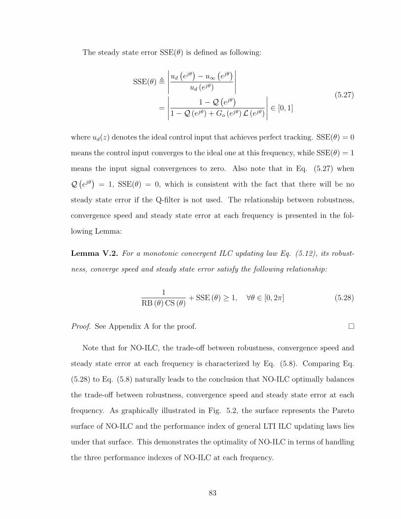
The steady state error SSE(θ) is defined as following:

SSE(θ) ,

∣∣∣∣∣ud(ejθ)− u∞

(ejθ)

ud (ejθ)

∣∣∣∣∣=

∣∣∣∣∣ 1−Q(ejθ)

1−Q (ejθ) +Go (ejθ)L (ejθ)

∣∣∣∣∣ ∈ [0, 1]

(5.27)

where ud(z) denotes the ideal control input that achieves perfect tracking. SSE(θ) = 0

means the control input converges to the ideal one at this frequency, while SSE(θ) = 1

means the input signal convergences to zero. Also note that in Eq. (5.27) when

Q(ejθ)

= 1, SSE(θ) = 0, which is consistent with the fact that there will be no

steady state error if the Q-filter is not used. The relationship between robustness,

convergence speed and steady state error at each frequency is presented in the fol-

lowing Lemma:

Lemma V.2. For a monotonic convergent ILC updating law Eq. (5.12), its robust-

ness, converge speed and steady state error satisfy the following relationship:

1

RB (θ) CS (θ)+ SSE (θ) ≥ 1, ∀θ ∈ [0, 2π] (5.28)


Note that for NO-ILC, the trade-off between robustness, convergence speed and

steady state error at each frequency is characterized by Eq. (5.8). Comparing Eq.

(5.28) to Eq. (5.8) naturally leads to the conclusion that NO-ILC optimally balances

the trade-off between robustness, convergence speed and steady state error at each

frequency. As graphically illustrated in Fig. 5.2, the surface represents the Pareto

surface of NO-ILC and the performance index of general LTI ILC updating laws lies

under that surface. This demonstrates the optimality of NO-ILC in terms of handling

the three performance indexes of NO-ILC at each frequency.

83

Note that the performance index of LTI ILC updating laws other than NO-ILC

still can lie on the Pareto curve/surface as shown in Fig. 5.6 and Fig. 5.2 for some

frequencies. The optimality of NO-ILC is that it guarantees the performance index

lies on the Pareto curve/surface over all the frequencies.

5.3 Conclusion

In this chapter, first, an analytical expression is derived to characterize the funda-

mental trade-off of NO-ILC between robustness, convergence speed and steady state

error. This equation can be leveraged to perform NO-ILC design considering the

fundamental trade-off explicitly and quantitatively. Thus, NO-ILC can be designed

according to different requirements, i.e., robustness, convergence speed and steady

state error, at different frequencies. This shows that the frequency dependent weight-

ing matrices design methodology discussed in Section 4.2 appears to be more powerful

than the diagonal weighting matrices design introduced in Section 4.1.

In the second part of this chapter, through a frequency domain analysis approach,

the allowable model uncertainty of general LTI ILC updating laws has been both

mathematically characterized and illustrated on the Nyquist plot, which helps the

RMC design if some knowledge of uncertainty range is given. In addition, the rela-

tionship between robustness, convergence speed and steady state error for general LTI

ILC updating laws is characterized at each frequency, which in turn demonstrates the

optimality of NO-ILC as the Pareto front as discussed in the first part of this chapter.

84

CHAPTER VI

Optimization Formulation towards NO-ILC Design

Chapter IV discusses the RMC analysis/design methodologies and Chapter VI

analytically lays out the fundamental trade-off of NO-ILC between robustness, con-

vergence speed and steady state error. Ideally, when designing NO-ILC, a robust

design with fast convergence and small steady state error is desired.

However, the design guidelines in Section 4.2.2 only provide general rules and

the design of the weighting matrices Q, R and S is still subject to manual tuning

at each frequency, which is ad-hoc and time consuming. So far, there is no design

method that explicitly considers the trade-off between robustness, convergence speed,

and steady state error and at the same time optimally balances that trade-off. This

chapter aims to fill this gap.

In order to fill the above identified gap, this section formulates the design of the

NO-ILC weighting matrices as an optimization problem to eliminate the manual tun-

ing process and avoid an unnecessarily conservative design. Specifically, this section

develops two optimization formulations to systematically design the weighting matri-

ces for NO-ILC, with one focusing on optimizing the nominal performance and the

other focusing on optimizing performance against all possible uncertainties.

85

6.1 Design for Optimal Nominal Performance

Even though the graphical criterion for RMC has been derived and the funda-

mental trade-off at each frequency has been laid out for NO-ILC in the previous

chapters, the filters W1(z), W2(z) and W3(z) still have to be designed manually to

satisfy the corresponding requirement at each frequency. The design guidelines are

summarized in Section 4.2.2. A systematic design approach, however, has not been

addressed yet. In this section, an optimization-based design methodology is proposed

for a systematic NO-ILC design for the purpose of ensuring RMC and at the same

time also taking the fundamental trade-off into account explicitly.

6.1.1 Problem Setup

Once the uncertainty has been formulated as described in Chapter III, the goal

is to design a NO-ILC that has RMC against all the possible modeling errors in

the uncertainty region while maximizing the convergence speed and minimizing the

steady state error. This needs to be done for all frequencies.

The graphical interpretation for RMC is to guarantee that the uncertainty region

on the Nyquist plot lies inside the RMC disk as illustrated in Fig. 4.18. Thus, at

each frequency θ, the radius r (θ) and center cx (θ) need to be appropriately chosen,

so that all edges of the uncertainty region lie inside the RMC disk.

Besides the robustness concern, the convergence speed and steady state error are

related to the radius and center of the disk as discussed in the rest of this section.

Note that the expressions for convergence speed and steady state error for nominal

performance are given as:

CS (θ) =|W1

(ejθ)|2|Go

(ejθ)|2 + |W3

(ejθ)|2

|W1 (ejθ) |2|Go (ejθ) |2 + |W2 (ejθ) |2 + |W3 (ejθ) |2

SSE (θ) =|W3

(ejθ)|2

|W1 (ejθ) |2|Go (ejθ) |2 + |W3 (ejθ) |2

(6.1)

86

which indicates that, for givenW1

(ejθ), maximizing the convergence speed is the same

as minimizing the value of∣∣W2

(ejθ)∣∣ and that minimizing the steady state tracking

error is the same as minimizing the value of∣∣W3

(ejθ)∣∣. Note that minimizing the

value of∣∣W2

(ejθ)∣∣ is equivalent to minimizing the radius of the RMC disk and the

radius is no smaller than one according to Eq. (4.25). Also, note the following

relationship:

r (θ)− cx (θ) =|W3

(ejθ)|2

|W1 (ejθ) |2|Go (ejθ) |2(6.2)

which indicates that minimizing the steady state tracking error is equivalent to min-

imizing the distance from the leftmost point on the RMC disk to the origin.

Thus, the original design problem is reformulated into a problem of designing the

appropriate radius and center of the RMC disk at various frequencies.

6.1.2 Optimization Setup to Design the Filters

In this section, the problem of designing a robust monotonic convergent NO-ILC

while maximizing convergence speed and minimizing steady state tracking error is

formulated as an optimization problem at a discrete set of points in the frequency

domain. Towards this end, after formulating the model uncertainty, the frequency

range is discretized with m points {θ1, . . . , θm}. For each frequency θi, the edges

of the uncertainty region are meshed with k points {(a1, b1) , . . . , (ak, bk)}, where aj

and bj denote the x and y coordinate of the jth meshed point on the edges of the

uncertainty region. A constrained optimization problem is then formulated at each

frequency θi as described in this section. To simplify the notation, cx,i and ri are used

to denote cx (θi) and r (θi).

87

6.1.2.1 Constrains

Two constraints are included in the optimization formulation. First, because of

the definition of the center and radius, Eq. (4.25), the following constraint holds:

ri ≥ ci ≥ 1, ∀i ∈ [1,m] (6.3)

Second, as discussed in the previous section, the edges of the uncertainty region

have to lie inside the RMC disk to achieve RMC. Mathematically, this condition is

expressed using the constraint

(aj − cx,i)2 + b2j ≤ σir

2i , ∀i ∈ [1,m], j ∈ [1, k] (6.4)

where σi ∈ (0, 1] is a safety factor introduced to compensate for the truncation error

that stems from the fact that the frequency domain analysis is for an infinite time

horizon, while in practice NO-ILC is always implemented in a finite time horizon.

Similar ideas can also be found in (Gorinevsky , 2002). The truncation error could be

small or even could be neglected for sufficiently large N , i.e., when N is significantly

larger than the length of the non-zero impulse response of Go(z), W1(z), W2(z) and

W3(z).

6.1.2.2 Cost Function

Besides RMC, faster convergence speed and smaller steady state tracking error

are also preferred. As per the discussion in Section 6.1.1, this goal is translated into

minimizing the radius while minimizing the distance from the leftmost point on the

RMC disk to the origin. Therefore, the following cost function is constructed:

Ji = αi‖ri − cx,i‖22 + ‖ri‖2

2, ∀i ∈ [1,m] (6.5)

88

where αi ≥ 0 is a tunable weighting factor. If αi is larger, the steady state error is

penalized more.

6.1.2.3 Solution Strategy

The fmincon command in Matlab is used in this thesis to solve the optimization

problem. At each frequency θi, the radius ri and center cx,i of the RMC disk is

optimized. Once the value of∣∣W1

(ejθi)∣∣ is determined (in this work it is chosen as

one), the values of∣∣W2

(ejθi)∣∣ and

∣∣W3

(ejθi)∣∣ are solved using ri, cx,i and

∣∣Go

(ejθ)∣∣

according to Eq. (4.25).

6.1.3 Least Squares Setup to Obtain the Weighting Matrices

After the optimization problem is solved,∣∣W1

(ejθi)∣∣, ∣∣W2

(ejθi)∣∣ and

∣∣W3

(ejθi)∣∣

are obtained for i ∈ [1,m]. Recall, however, that the ultimate goal is to obtain the

weighting matrices Q, R and S. This section describes how the weighting matrices

can be obtained from∣∣W1

(ejθi)∣∣, ∣∣W2

(ejθi)∣∣ and

∣∣W3

(ejθi)∣∣ using a least squares

formulation.

Note that the weighting matrices Q, R and S are lifted representations of the zero

phase filtersQ(z) = W1(z−1)W1(z), R(z) = W2(z−1)W2(z) and S(z) = W3(z−1)W3(z).

Also note that∣∣Q (ejθ)∣∣ =

∣∣W1

(ejθ)∣∣2,

∣∣R (ejθ)∣∣ =∣∣W2

(ejθ)∣∣2 and

∣∣S (ejθ)∣∣ =∣∣W3

(ejθ)∣∣2. The matrix Q and the zero-phase filter Q(z) have the following structure:

Q =

q0 q1 · · · qN−1

q1 q0 q1...

... q1. . . q1

qN−1

· · · q1 q0

∈ RN

Q(z) = · · ·+ q2z2 + q1z + q0 + q1z

−1 + q2z−2 + · · ·

(6.6)

Similar structures hold for R, R(z) and S, S(z), as well.

89

For a stable filter, qi

will be zero for some sufficiently large i, since the impulse

response of a stable system will decay to zero. Thus, for sufficiently large N , the

following relationship is true:

Q(ejθ)

=∣∣W1

(ejθ)∣∣2 ≈ N−1∑

i=−(N−1)

q|i|ejiθ =

N−1∑i=1

2qicosiθ + q0 (6.7)

For practical concerns, when N is significantly larger than the time steps that

needed for the impulse response to decay to zero, the above equation can be a good

approximation. Thus, the following least squares problem is formulated:

∣∣W1

(ejθ1)∣∣2∣∣W1

(ejθ2)∣∣2

...∣∣W1

(ejθm

)∣∣2

=

1 2 cos θ1 · · · 2 cos (N − 1) θ1

1 2 cos θ2 · · · 2 cos (N − 1) θ2

......

......

1 2 cos θm · · · 2 cos (N − 1) θm

q0

q1...

qN−1

(6.8)

To have a unique solution to this least squares problem, using m ≥ N is preferred.

Once the solution is obtained, the construction of the weighting matrix Q is complete.

R and S matrices are obtained using the same method.

This completes the description of the design methodology for optimal nominal

performance. This design methodology guarantees RMC against possible uncertain-

ties while maximizing the convergence speed and minimizing the steady steady state

error for optimal nominal performance. However, note that a better nominal perfor-

mance does not necessarily correspond to a better performance when uncertainty is

present. Therefore, the following section presents an alternative design methodology

that guarantees RMC while maximizing the convergence speed and minimizing the

steady steady state error for optimal performance under the presence of uncertainties.

90

6.2 Design for Optimal Performance Under Uncertainties

An optimal design for the nominal plant does not necessarily guarantee a good

performance for the real plant. In this section, two examples are used to demonstrate

this fact first. Then, the optimization problem formulation of the previous section

is modified to create a design method for optimal performance against uncertainties

while ensuring RMC.

6.2.1 Disadvantage of the Nominal Performance Based Design

The two examples given in this section illustrate the fact that increasing R does

not necessarily slow down the convergence speed and increasing S does not necessarily

increase the steady state error against a modeling error. All the transfer functions

are reported in continuous domain for ease of presentation, but are discretized with

a sampling time of Ts = 0.01s in the implementation. In both examples, the tracking

reference is a sinusoid with a frequency of 30.1 rad/s.

Example 1: Consider the nominal plant and the modeling error

Go(s) =s+ 1

s+ 2; Ue(s) = 1.8

s+ 11

s+ 10(6.9)

Consider two weighting matrix designs for NO-ILC. Design 1 is with Q1 = I, R1 =

S1 = 0, and Design 2 is with Q2 = R2 = I, S2 = 0, where I represents the iden-

tity matrix. Both designs in this case guarantee RMC against the modeling error

Ue(s). Considering the nominal performance for both designs, Design 1 has a faster

convergence speed, since R1 < R2. However, Design 1 converges much slower in the

presence of the modeling error as shown in Fig. 6.1(a).

Example 2: Consider the nominal plant and modeling error

Go(s) =s+ 1

s+ 2; Ue(s) = −0.2 (6.10)

91

10 15 20 25 30 35 400

5

10

15

20

25

30

35

40

Design 1

Design 2

80 10020

40

60

80

100

120

140

160

180

200Example 1 Example 2

Iteration Number Iteration Number( )a ( )b

Design 1

Design 2

2e

2e

50 0 20 40 60

Figure 6.1: Two examples illustrating that better nominal performance does not nec-essarily mean better performance against model uncertainty

Consider two weighting matrix designs for NO-ILC. Design 1 is with Q1 = I, R1 = 0,

S1 = 0.25I, and Design 2 is with Q2 = I, R2 = 0, S2 = 0.5I. Both designs in

this case guarantee RMC against the modeling error Ue(s). Considering the nominal

performance for both designs, Design 1 has a smaller steady state error, since S1 < S2.

However, Design 1 leads to a much larger steady state error when the modeling error

is present as shown in Fig. 6.1(b).

The above two examples show that improving the nominal performance of NO-ILC

does not necessarily lead to a better performance against model uncertainty. There-

fore, the performance of the design that results from the optimization formulation

developed in the previous section may have limitations. An alternative formulation is

presented in this section that aims to maximize the performance of NO-ILC against

model uncertainties.

6.2.2 Design Against Uncertainties

To ensure the robustness of NO-ILC against model uncertainty, the gray uncer-

tainty region on Nyquist plot needs to lie inside the RMC disk over all frequencies.

92

This goal is the same as the one in the nominal performance based design. To maxi-

mize the convergence speed and minimize the steady state error against all possible

model uncertainty, however, the specific goal of the optimization is modified. In

particular, the following two terms need to be minimized at each frequency θi:

CRu :=∣∣Q (ejθi)− L (ejθi)G (ejθi)∣∣2 (6.11)

SSEu :=

∣∣∣∣∣ 1−Q(ejθi)

1−Q (ejθi) + L (ejθi)G (ejθi)

∣∣∣∣∣2

(6.12)

where CRu is the convergence rate and SSEu is steady state error against the model

uncertainty. Recall that G(ejθi)

= Go

(ejθi)Ue(ejθi). Even though Ue

(ejθi)

is un-

known, its range is known as the gray region illustrated in Fig. 4.18 at frequency θi.

In this alternative formulation, this gray region is meshed uniformly with p points

{Ue,1(ejθi), · · · , Ue,p

(ejθi)} in addition to meshing the edges as in the previous for-

mulation. Let

xii = Re{Ue,ii(ejθi)}, yii = Im{Ue,ii(ejθi)}, ii ∈ [1, p] (6.13)

where Re{·} and Im{·} denote the real part and imaginary part of a complex number.

For simplicity of notation, Qi, Li and Go,i are used to denote Q(ejθi), L(ejθi)

and

Go

(ejθi), respectively. Assuming Ue

(ejθi)

has equal chance to lie anywhere inside the

uncertainty region, minimizing Eq. (6.11) and Eq. (6.12) is the same as minimizing

the following expressions:

p∑ii=1

(Qi − LiGo,i (xii + jyii)) (Qi − LiGo,i (xii − jyii)) (6.14)

p∑ii=1

1−Qi1−Qi + LiGo,i (xii + jyii)

× 1−Qi1−Qi + LiGo,i (xii − jyii)

(6.15)

93

Note the following relationship between ri, cx,i, Qi and LiGo,i:

Qi =cx,iri

; LiGo,i =1

ri(6.16)

Plugging the above equations into Eq. (6.14) and (6.15) leads to the cost function

for the optimal design against uncertainties at each frequency θi:

Ji =

p∑ii=1

(xii − cx,i)2 + yii2

ri2+ αi

p∑ii=1

(ri − cx,i)2

(xii + ri − cx,i)2 + yii2(6.17)

where αi ≥ 0 is a tunable weighting factor.

The constraint formulations and the solution strategy are the same as the previous

formulation. Hence, this design approach differs from the previous one in only two

ways: 1) the uncertainty region is meshed in addition to the edges; and 2) a different

cost function is used in the optimization.

If there is some prior knowledge about where Ue(ejθi)

is more likely to lie in the

uncertainty region, weighting factors can be introduced in Eq. (6.14) and Eq. (6.15)

to incorporate that knowledge.

6.3 Summary of Design Procedure

Step 1: Formulate the model uncertainty, pick m frequencies {θ1, · · · , θm} with

m ≥ N . For each frequency θi, mesh the edges of the uncertainty region with k points

{(a1, b1) , · · · , (ak, bk)}. Additionally, if designing for an optimal performance against

uncertainties, mesh the uncertainty region with p points {(x1, y1) , · · · , (xp, yp)} at

each frequency θi, as well.

Step 2: For each frequency θi, solve the constrained optimization with the cost

function of Eq. (6.5) for optimal nominal performance or Eq. (6.17) for optimal

performance against uncertainties and constrains of Eq. (6.4), (6.3). Based on the

94

obtained radius ri and center cx,i of the RMC disk at each frequency, determine∣∣W1

(ejθi)∣∣, ∣∣W2

(ejθi)∣∣ and

∣∣W3

(ejθi)∣∣.

Step 3: Solve the least squares problem as shown in Eq. (6.8), to obtain the

weighting matrices Q, R and S.

6.4 Simulation Examples

Two simulation examples are used to demonstrate the effectiveness of the devel-

oped design methodologies. The first example compares the performances of the two

design methodologies presented above. The second example focuses on the design for

optimal performance under uncertainties and shows how the weighing term α affects

the trade-off between convergence speed and steady state error. All the transfer func-

tions are reported in continuous domain, but are discretized in the implementation

with a sampling time of Ts = 0.01s. The number of total running steps is N = 3000.

6.4.1 Example 1

Consider the following nominal plant and modeling error:

Go(s) =s+ 20

s+ 5; Ue(s) =

(0.19s+ 1) (0.033s+ 1)

(0.08s+ 1) (0.05s+ 1)(6.18)

Let the upper and lower bounds on the Bode plot be

Ue,max(s) = 3s+ 5

s+ 10; Ue,min(s) = 0.3

s+ 20

s+ 10(6.19)

The Bode plot of the real system G(s) = Go(s)Ue(s) is shown as the dotted red curve

in Fig. 6.2. The nominal plant Go(s) is shown as the solid green curve. The upper

and lower bounds of the uncertainty region are indicated as the dashed blue lines in

Fig. 6.2 and the gray region indicates the uncertainty region.

95

Mag

nit

ud

e (d

B)

-20

-10

0

10

20

10-1

100

101

102

103

Ph

ase

(deg

)

-60

-30

0

Bode Diagram

Frequency (rad/s)

( )minG z

( )maxG z

Uncertainty Bounds

System Model

Uncertainty Range

Real System

Figure 6.2: Bode plot of the real system, nominal model and uncertainty range

Design for Optimal Nominal Performance (Design 1): The frequency range

of interest in this case is uniformly meshed into m = 3000 points {θ1, · · · , θm} with

θ1 = 0 and θm = π/Ts rad/s. For each frequency θi, the edges of the uncertainty

region are meshed with k = 100 points, with 25 points on each edge. For example,

the meshed points are shown in Fig. 6.3a at the frequency of 15 rad/s. For the

optimization setup, the safety factor σi is set to 0.9 and the weighting factor αi is

set to 100 for all i ∈ [1,m]. At each frequency θi, the radius ri and the center cx,i

are optimized. As an example, the RMC disks obtained at 15 rad/s and 73 rad/s are

shown as the green circles in Fig. 6.4a and Fig. 6.4b.

Design for Optimal Performance Under Uncertainties (Design 2): In

this example, the number of the meshing points in the uncertainty region is picked as

p = 100. As an example, the meshing of the uncertainty region at 15 rad/s is shown

in Fig. 6.3. All the other settings remain the same as in Design 1. As an example,

the RMC disks obtained at 15 rad/s and 73 rad/s are shown as the cyan circles in

Fig. 6.4a and Fig. 6.4b.

96

0 0.5 1 1.5 2 2.5 3

-1

-0.5

0

0.5

1

( ),j ja b

,max ( )eU z

( )eU z

,min ( )eU z

0 0.5 1 1.5 2 2.5 3

-1

-0.5

0

0.5

1,max ( )eU z

( )eU z

,min ( )eU z

( ),ii iix y

Real Axis Real Axis

Imag

inar

y A

xis

Imag

inar

y A

xis

( )a ( )b

Figure 6.3: Mesh points of the (a) edges of uncertainty region and (b) uncertaintyregion at 15 rad/s

2 3 5

-2

-1.5

-1

-0.5

0

0.5

1

1.5

2

Real Axis

Imag

inar

y A

xis

Real Axis

Imag

inar

y A

xis

( )a ( )b

RMC Disk for Design 1 RMC Disk for Design 2

( ) ( ),max ,min;e eU z U z

0 1 4

-2

-1.5

-1

-0.5

0

0.5

1

1.5

2

2 3 50 1 4

( )eU z ( )jeU e θ

Figure 6.4: RMC disks for Design 1 and Design 2 at (a) 15 rad/s and (b) 73.2 rad/s

97

10 15 20 25 300

5

10

15

20

25

30

35

40

Iteration Number

2 N

orm

of

Tra

ckin

g E

rror

0

5

10

15

20

25

30

35

40

2 N

orm

of

Tra

ckin

g E

rror

Iteration Number

( )a ( )b

50 10 15 20 25 3050

Tracking Performance foro

G Tracking Performance forG

2Design 2, 0.53

o− GQ L =

2Design 1, 0.37

o− GQ L =

2Design 2 4, 0.4− GQ L =

2Design 1 0, 0.8− GQ L =

Figure 6.5: Tracking performance against (a) nominal plant and (b) real plant

The tracking reference is a sinusoid of 15 rad/s. Fig. 6.5a shows the tracking

results for the nominal plant Go, whereas Fig. 6.5b shows the tracking results for

the real plant Go. For both cases, since the penalty for steady state error in the

cost function is set to a large number (αi = 100) and since the model uncertainty is

positive real (the phase of the uncertainty region never exceeds [0,−π/2] in Fig. 6.2),

the RMC disks generated by both design methods never go to the left half plane. This

corresponds to a design with no Q-filter. As a result, zero steady state tracking error

is achieved with both design formulations as shown in Fig. 6.5, and the difference

between the two formulations manifests itself in the convergence speed.

With nominal performance being its focus, Design 1 always seeks the smallest disk

that encloses the uncertainty region. Thus, the RMC disks obtained by Design 1 are

smaller than those obtained by Design 2; see Fig. 6.4 for examples at two frequencies.

As a result, Design 1 converges faster than Design 2 for the nominal plant as seen

in Fig. 6.5a. However, better nominal performance does not necessarily mean better

performance in the presence of uncertainties. Fig. 6.5b shows the tracking results of

the two design methods for the real plant. Both methods ensure RMC as expected.

98

Mag

nit

ud

e (d

B)

-30

-20

-10

0

10

20

10-2

10-1

100

101

102

103

Ph

ase

(deg

)

-90

-45

0

Bode Diagram

Frequenc y (rad/s)

Uncertainty Bounds

System Model

Uncertainty Range

Real System

( )maxG z

( )minG z

Figure 6.6: Bode plot of the real system, nominal model and uncertainty range

However, Design 2 converges faster than Design 1, which is consistent with the fact

that Design 2 specifically targets optimal performance against uncertainties.

6.4.2 Example 2

In this example, the functionality of the weighting term α is illustrated. Consider

the following nominal plant and modeling error:

Go(s) =s+ 20

s+ 5; Ue(s) = 0.95

(0.45s+ 1) (0.45s+ 1)

(1.5s+ 1) (2.5s+ 1)(6.20)

Let the upper and lower bounds on the Bode plot be

Ue,max(s) =1.95s+ 13

s+ 10; Ue,min(s) =

(3.6s+ 8) (4.5s+ 10)

(15s+ 10) (25s+ 10)(6.21)

The Bode plot of the real system, system model and uncertainty region are shown in

Fig. 6.6.

We consider the design for optimal performance under uncertainties (Design 2).

99

Similar to the previous example, the frequency range of interest is uniformly meshed

into m = 3000 points {θ1, . . . , θ2} with θ1 = 0 and θm = π/Ts rad/s. For each

frequency θi, the edges of the uncertainty region are meshed with k = 100 points,

with 25 points on each edge, and the number of the meshing points in the uncertainty

region is picked as p = 100. For the optimization setup, the safety factor σi i is set

to 0.985 and the weighting factor αi is picked from a list of {2, 4, 8, 16, 32} for all

i ∈ [1,m].

In this case, the model uncertainty is still positive real, since the phase difference

never exceeds [0,−π/2] as shown in Fig. 6.6. However, the uncertainty region does

get very close to the imaginary axis at the frequency around 1.5 rad/s; as an example,

see the gray uncertainty region in Fig. 6.7 at 1.47 rad/s. To enclose this uncertainty

region, the RMC disk can be picked either with a smaller radius but with larger area

in the negative half plane (e.g., see the RMC disk for α = 2 in Fig. 6.7), or with a

larger radius but smaller area in the negative half plane (e.g., see the RMC disk for

α = 32 in Fig. 6.7). The RMC disks generated by different α values at this frequency

are shown in Fig. 6.7 with a zoom-in view around the origin showing how much the

RMC disk goes into the negative half plane for different α values.

The tracking reference is a sinusoid of 1.5 rad/s. For different values of α, the

tracking results are shown in Fig. 6.8. All designs yield RMC, since the tracking

differences ei − e∞ are monotonic convergent as shown in Fig. 6.8b. As expected,

larger α value corresponds to more penalization on the steady state error and therefore

leads to smaller steady state error as shown in Fig. 6.8a, however, at the cost of slower

convergence speed as shown in Fig. 6.8b.

6.5 Conclusion

This chapter contributes in two aspects to the NO-ILC literature. First, an op-

timization approach is developed for designing the NO-ILC weighting matrices that

100

Real Axis

-1 0 1 2 3 4 5 6

Imag

inar

y A

xis

-2.5

-2

-1.5

-1

-0.5

0

0.5

1

1.5

2

2.5

0

-0.05 0

-0.02

0.02

2α = 4α =

8α = 16α = 32α =

( ) ( ),max ,min;e e

U z u z ( )eU z ( )je

U eθ

Figure 6.7: RMC disks for different α values at 1.47 rad/s

Tracking Error:i

−r y

0 200 400 600 800 10000

5

10

15

20

25

30

35

40

0 200 400 600 800 10000

5

10

15

20

25

30

35

40

2 N

orm

of

Tra

ckin

g D

iffe

rence

Iteration Number

( )b

2 N

orm

of

Tra

ckin

g E

rror

Iteration Number

( )a

2α =

4α =

8α =

16α =

32α =

Tracking Difference:i ∞−e e

22, 0.9697α = − GQ L =

24, 0.9830α = − GQ L =

28, 0.9911α = − GQ L =

216, 0.9950α = − GQ L =

232, 0.9966α = − GQ L =

Figure 6.8: Design for optimal performance under uncertainties (a) tracking error and(b) tracking difference

101

eliminates the manual tuning process for filter designs and systematically achieves an

optimal balance between robustness, convergence speed and steady state error. Sec-

ond, two different optimization formulations are constructed. Both formulations aim

for RMC, but the first one seeks to optimize the nominal performance, whereas the

second one seeks to optimize the performance against uncertainties. The proposed

design approach is shown through two demonstrative examples to be an effective,

systematic procedure for designing NO-ILC.

102

CHAPTER VII

Concluding Remarks and Future Work

This thesis aims to answer the question of: Can we develop analysis and design

tools that better characterize the allowable model uncertainties and better reveal the

frequency domain properties of NO-ILC?

The objective of this research is to provide fundamental analysis tools for the

frequency domain properties of Norm-Optimal Iterative Learning Control (NO-ILC),

which leads to novel design methodologies for NO-ILC to compensate the trade-off

between robustness, convergence speed and steady state error at different frequencies.

The work presented in Chapters III to VI results in the following contributions to the

NO-ILC literature:

• This work presents a new model uncertainty formulation for NO-ILC. Unlike

the conventional uncertainty formulation, which leads to the conclusion that

R does not affect the robustness (Donkers et al., 2008; Gorinevsky , 2002), the

new formulation used in this work yields that the robustness is affected by both

R and S, but in different manners. This is partially based on the following

publications:

Ge, X., J. L. Stein, and T. Ersal (2016a), A frequency domain ap-

proach for designing filters for norm-optimal iterative learning control

and its fundamental tradeoff between robustness, convergence speed

103

and steady state error, American Control Conference, pp. 384–391

Ge, X., J. L. Stein, and T. Ersal (2017a), Frequency domain analysis

of robust monotonic convergence of norm-optimal iterative learning

control, IEEE Transactions on Control System Technology, accepted

• Based on the above uncertainty formulation, this work both mathematically

and graphically presents how the weighting terms in the cost function affect the

robustness of NO-ILC. This leads to several new graphical design methodologies

for the weighting matrices to achieve the RMC requirement. This is partially

based on the following publications:





Ge, X., J. L. Stein, and T. Ersal (2017b), A frequency-dependent fil-

ter design approach for norm-optimal iterative learning control and

its fundamental trade-off between robustness, convergence speed and

steady state error, ASME Journal of Dynamic Systems, Measure-

ment and Control, submitted

• An analytical equation is derived to quantitatively characterize the fundamental

trade-off between robustness, convergence speed and steady state error of NO-

ILC in frequency domain. This equation can be helpful during the design process

to satisfy a desired robustness requirement while ensuring fast convergence and

small steady state error at different frequencies. This equation also reveals the

optimality of NO-ILC among general ILC updating laws in the scope of LTI

104

systems. And this is partially based on the following publications:





Ge, X., J. L. Stein, and T. Ersal (2017b), A frequency-dependent fil-

ter design approach for norm-optimal iterative learning control and

its fundamental trade-off between robustness, convergence speed and

steady state error, ASME Journal of Dynamic Systems, Measure-

ment and Control, submitted

Ge, X., J. L. Stein, and T. Ersal (2017d), Optimality of norm-optimal

iterative learning control, ASME Journal of Dynamic Systems, Mea-

surement and Control, to be submitted

• Based on the analysis on allowable model uncertainty and fundamental trade-off

for NO-ILC, two optimization based formulations are proposed to systematically

design the weighting matrices for NO-ILC, which eliminate the manual tuning

process and avoid unnecessarily conservative designs. And this is partially based

on the following publications:

Ge, X., J. L. Stein, and T. Ersal (2016b), Optimization based weight-

ing matrices design for norm optimal iterative learning control, Dy-

namics Systems and Control Conference

Ge, X., J. L. Stein, and T. Ersal (2017c), Optimization based weight-

ing matrices design for norm optimal iterative learning control, IEEE

Transactions on Control System Technology, to be submitted

105

Specifically, Chapter III proposes a novel model uncertainty formulation on Bode

Plot and addresses the transformation of this uncertainty between the Bode and

Nyquist plots. Then the validity of frequency domain RMC criterion is addressed and

the need for new graphical design methodology is motivated. Based on the proposed

model uncertainty formulation, Chapter IV presents two novel RMC analysis and

design tools for NO-ILC, one with diagonal weighting matrices design and the other

one with frequency dependent weighting matrices design. Both analysis methods offer

graphical interpretations of the allowable model uncertainty region on the Nyquist

plot and lead to novel design guidelines, which are less conservative compared with the

traditional NO-ILC design methods. Chapter V develops an analytical equation that

characterizes the fundamental trade-off of NO-ILC between robustness, convergence

speed and steady state error at each frequency. Furthermore, it shows that NO-ILC

is the optimal solution under the scope of general LTI ILC updating laws for LTI

systems in terms addressing the trade-off between robustness, convergence speed and

steady state error at each frequency. Chapter VI presents two different formulations

for the design of NO-ILC weighting matrices as an optimization problem to eliminate

the manual tuning process and avoid unnecessary conservative designs.

The developed analysis and design methodologies currently are for SISO systems.

One potential interesting future research direction is to extend the current analysis

and design tools to MIMO systems. As mentioned, NO-ILC is originally derived

using the lifted representation. The current research adopts the transfer function

representation to better address the frequency domain properties of NO-ILC. Another

interesting potential research direction is to explore whether adopting the state-space

representation in NO-ILC analysis/design would further reveal other properties of

NO-ILC.

106

APPENDICES

107

APPENDIX A

PROOFS FOR PROPOSITIONS AND LEMMAS

Proof of of Proposition IV.1:

Proof. Because 0 < α (θ) ≤ 1 and∣∣Ue (ejθ)∣∣2 ≥ 0, to satisfy the criterion given by

Eq. (4.2), Re{Ue(ejθ)} needs to be non-negative for all θ ∈ [0, 2π]. If Re{Ue

(ejθ)}

is negative for any θ ∈ [0, 2π], Criterion (4.2) cannot be satisfied.

Proof of Proposition IV.2:

Proof. If for λ0 the NO-ILC is robust monotonic convergent, then Re{Ue(ejθ)} > 0

for all θ ∈ [0, 2π] and the following inequality is valid:

CR0 (θ) = (α0 (θ))2∣∣Ue (ejθ)∣∣2 − 2α0 (θ) Re{Ue

(ejθ)} < 0 (A.1)

where CR (θ) stands for convergence ratio. Note that CR (θ) > −1 and CR (θ) ∈

(−1, 0) for RMC. α0 (θ) is defined as

α0 (θ) ,

∣∣Go

(ejθ)∣∣2

|Go (ejθ)|2 + λ0

(A.2)

108

If a λ′ > λ0 is chosen for NO-ILC, the RMC criterion becomes

CR′ (θ) = (α′ (θ))2∣∣Ue (ejθ)∣∣2 − 2α′ (θ) Re{Ue

(ejθ)} < 0 (A.3)

where α′ (θ) is defined as

α′ (θ) ,

∣∣Go

(ejθ)∣∣2

|Go (ejθ)|2 + λ′(A.4)

Because α0 (θ) ∈ (0, 1], from Eq. (A.1) it can be shown that

−2Re{Ue(ejθ)} < −α0 (θ)

∣∣Ue (ejθ)∣∣2 (A.5)

Substituting Eq. (A.5) into CR′, the following inequality is obtained:

CR′ (θ) < α′ (θ) (α′ (θ)− α0 (θ))∣∣Ue (ejθ)∣∣2 < 0 (A.6)

Therefore, CR′ (θ) < 0 for all θ ∈ [0, 2π].

Proof of Lemma IV.3:

Proof. If Ue(eθ)

lies inside the RMC disk for all θ ∈ [0, 2π], this means Eq. (4.5) is

valid; i.e.

a2(x2 (θ) + y2 (θ)

)− 2ax < 0 (A.7)

Substituting the definitions of x (θ) and y (θ) into the above equation gives Eq.

(A.8).

(a

α (θ)

)2 [(α (θ))2

∣∣Ue (ejθ)∣∣2 − 2α (θ) Re{Ue(ejθ)}]

+ 2a

[a

α (θ)− 1

]Re{Ue

(ejθ)} < 0,∀θ ∈ [0, 2π] (A.8)

109

Note that with β = 0 the disk lies in the right half plane; thus Re{Ue(ejθ)} ≥ 0.

Combing this observation with the fact that 1 > a ≥ α (θ) > 0, the following is

obtained:

(α (θ))2∣∣Ue (ejθ)∣∣2 − 2α (θ) Re{Ue

(ejθ)} < 0,∀θ ∈ [0, 2π] (A.9)

The above inequality is exactly the same as the RMC Criterion (4.2). Therefore,

the NO-ILC as described by Eq. (2.15) with β = 0 is robust monotonic convergent

against the modeling error Ue (z).

The above analysis shows that Eq. (4.5) is a sufficient condition for Criterion

(4.2). In addition, as per the discussion after Eq. (4.5), a larger λ value enlarges the

RMC region. Hence, using λ′ > λ0 would enlarge the RMC region.


Proof. If the modeling error Ue (z) can be tolerated with λ = λ0 and β = 0, Eq. (4.7)

holds with α (θ) = γ (θ) and can be written as Eq. (A.10).

[α (θ)

γ (θ)

]2 [γ2 (θ)

∣∣Ue (ejθ)∣∣2 − 2γ2 (θ)

α (θ)Re{Ue

(ejθ)}+

γ2 (θ)

α2 (θ)− 1

]+

[α (θ)

γ (θ)

]2(1− γ2 (θ)

α2 (θ)

)< 0,∀θ ∈ [0, 2π] (A.10)

When λ is held at the same value and β is increased from 0, according to the

definition of γ (θ) and α (θ), the following always holds: 0 < γ (θ) < α (θ) < 1.

Substituting these relationships into Eq. (A.10) implies Eq. (4.7), since the second

term in Eq. (A.10) is positive. This means this modeling error can also be tolerated

with λ = λ0 and β > 0.


110

Proof. If for λ0 and β0 the NO-ILC has RMC against Ue (z), Eq. (A.11) holds

CR0 (θ) , γ20 (θ)

∣∣Ue (ejθ)∣∣2 − 2γ2

0 (θ)

α0 (θ)Re{Ue

(ejθ)}+

γ20 (θ)

α20 (θ)

− 1 < 0, ∀θ ∈ [0, 2π]

(A.11)

where α0 (θ) and γ0 (θ) are defined in Eq. (4.3) and Eq. (4.6), respectively. Following

the definition of x (θ) and y (θ) in Eq. (4.4), after some manipulation, Eq. (A.11)

can be re-written into Eq. (A.12). Following the same argument as in Proposition

IV.1, x (θ)−(α−1

0 (θ)− γ−10 (θ)

)needs to be non-negative for all θ ∈ [0, 2π].

CR0 (θ) = γ20 (θ)

[(x (θ)−

(1

α0 (θ)− 1

γ0 (θ)

))2

+ y2 (θ)

]

− 2γ0 (θ)

[x (θ)−

(1

α0 (θ)− 1

γ0 (θ)

)]< 0,∀θ ∈ [0, 2π] (A.12)

If λ0 is increased to λ′ but β0 retains its value, the convergence ratio, CR′ (θ),

becomes Eq. (A.13):

CR′ (θ) = (γ′ (θ))2

[(x (θ)−

(1

α′ (θ)− 1

γ′ (θ)

))2

+ y2 (θ)

]

− 2γ′ (θ)

[x (θ)−

(1

α′ (θ)− 1

γ′ (θ)

)](A.13)

Note the following relationship:

1

α′ (θ)− 1

γ′ (θ)=

1

α0 (θ)− 1

γ0 (θ)= − β0

|Go (ejθ)|2(A.14)

From Eq. (A.12) it follows that

2

γ0 (θ)

(x (θ) +

β0

|Go (ejθ)|2

)>

(x (θ) +

β0

|Go (ejθ)|2

)2

+ y2 (θ) (A.15)

Substituting Eq. (A.15) into Eq. (A.13) and knowing that 0 < γ′ (θ) < γ0 (θ) ≤ 1

111

leads to Eq. (A.16) as shown in the next page. Therefore, CR′ (θ) < 0 is true for

any θ ∈ [0, 2π]. This completes the proof of the argument that if the modeling error

Ue (z) can be tolerated with certain λ and β values, NO-ILC has RMC at least for

the same Ue (z) with a larger λ value.

CR′ (θ) <

[(x (θ) +

β0

|Go (ejθ)|2

)2

+ y2 (θ)

]γ′ (θ) (γ′ (θ)− γ0 (θ)) < 0,∀θ ∈ [0, 2π]

(A.16)

Reconsider CR0 (θ) in Eq. (A.11); it can be re-written as

CR0 (θ) = γ20 (θ)

(x2 (θ) + y2 (θ)

)− 2

γ20 (θ)

α0 (θ)x+

γ20 (θ)

α20 (θ)

− 1 (A.17)

If β0 is increased to β′ but λ0 retains its value, the RMC criterion becomes the

following, for all θ ∈ [0, 2π]

CR′ (θ) = (γ′ (θ))2 (x2 (θ) + y2 (θ)

)− 2

(γ′ (θ))2

α0 (θ)x+

(γ′ (θ)

α0 (θ)

)2

< 1 (A.18)

Subtracting CR′ (θ) from CR0 (θ) gives:

CR′ (θ)− CR0 (θ) =

((γ′ (θ)

γ0 (θ)

)2

− 1

)(CR0 (θ) + 1) (A.19)

Because CR0 (θ) ∈ (−1, 0), the inequality CR′ (θ) < CR0 (θ) < 0 is true for any

θ ∈ [0, 2π]. This completes the proof of the argument that if the modeling error Ue (z)

can be tolerated with certain λ and β values, NO-ILC still has RMC at least for the

same Ue (z) with a larger β value.

Note that it has been proved that:

• Increasing λ and retaining β will not degrade the RMC region.

• Increasing β and retaining λ will not degrade the RMC region.

112

If both λ and β are increased from λ0 and β0, the following statement follows

immediately from the two statements above:

• Increasing both λ and β will not degrade the RMC region.

Combining the above three statements completes the proof.

Proof of Lemma IV.6:

Proof. If Ue(eθ)

lies inside the RMC disk for all θ ∈ [0, 2π], this means Eq. (4.10) is

valid. After some manipulations Eq. (4.10) leads to Eq. (A.20) for all θ ∈ [0, 2π] .

Since the terms T2 and T3 are positive, the term T1 must be negative, which translates

to Criterion (4.1) after plugging in the definition of x (θ), y (θ), α (θ) and γ (θ).

T1 + T2 + T3 < 0, ∀θ ∈ [0, 2π]

T1 =

[x (θ)−

(1

α (θ)− 1

γ (θ)

)]2

− 2

γ (θ)

[x (θ)−

(1

α (θ)− 1

γ (θ)

)]+ y2 (θ)

T2 =

[(1

a− 1

q

)−(

1

α (θ)− 1

γ (θ)

)][2

γ (θ)−(

1

α (θ)− 1

γ (θ)

)−(

1

a− 1

q

)]

T3 =

[x (θ)−

(1

a− 1

q

)](2

α (θ)− 2

a

)(A.20)

The above analysis shows that Eq. (4.10) is a sufficient condition for Criterion

(4.1). In addition, as per the discussion after Eq. (4.10), either a larger λ or a larger

β value enlarges the RMC region, but in a different manner. Hence, using λ′ > λ0 or

β′ > β0 would enlarge the RMC region.

113

Proof of Proposition V.1:

Proof. Note that RB−1 (θ) equals to∣∣Go

(ejθ)L(ejθ)∣∣, which is the length of the red

vector in Fig. 5.6. It is also easy to see that the length of the blue vector in Fig.

5.6 equals to the value of convergence ratio CR (θ). From geometry, the following

equation is true:

∣∣Go

(ejθ)L(ejθ)∣∣+

∣∣1−Go

(ejθ)L(ejθ)∣∣ ≥ 1,∀θ ∈ [0, 2π) (A.21)

since the shortest distance between the two points in Fig. 5.6, (0,0) and (1,0), is

the line that directly connects them, whose length is 1. The above inequality can be

re-written into:

1

RB (θ)+ CR (θ) ≥ 1, ∀θ ∈ [0, 2π) (A.22)

Substituting Eq. (5.20) into the above equation gives Eq. (5.21). This is completes

the proof.

Proof of Proposition V.2:

Proof. For simplicity, the(ejθ)

term will be omitted in the proof, i.e., Q and GoL

are used to denote Q(ejθ)

and Go

(ejθ)L(ejθ). Note that the following relationship

is true:

1− |Q −GoL| ≤ |1− (Q−GoL)| , ∀θ ∈ [0, 2π] (A.23)

For a monotonic convergent ILC updating law, |Q −GoL| < 1 for all θ ∈ [0, 2π].

Therefore, the following is true:

1

1− |Q −GoL|≥ 1

|1− (Q−GoL)|, ∀θ ∈ [0, 2π] (A.24)

114

Multiplying both sides by |GoL| gives the following inequality for all θ ∈ [0, 2π]:

|GoL|1− |Q −GoL|

≥ |GoL||1−Q+GoL|

=

∣∣∣∣ GoL1−Q+GoL

∣∣∣∣ (A.25)

Adding SSE(θ), Eq. (5.27), to both sides of the above inequality gives:

∣∣∣∣ 1−Q1−Q+GoL

∣∣∣∣+|GoL|

1− |Q+GoL|≥∣∣∣∣ 1−Q

1−Q+GoL

∣∣∣∣+

∣∣∣∣ GoL1−Q+GoL

∣∣∣∣ ≥∣∣∣∣1−Q+GoL1−Q+GoL

∣∣∣∣ = 1 (A.26)

Since RB−1(θ) = |GoL| and CS(θ) = 1− |Q −GoL| according to their definitions

Eq. (5.26), the above inequality can be re-written as Eq. (5.28). This is completes

the proof.

115

BIBLIOGRAPHY

116

BIBLIOGRAPHY

Ahn, H. S., K. Moore, and Y. Chen (2005), Schur stability radius bounds for robustiterative learning controller design, American Control Conference, pp. 178–183.

Ahn, H. S., Y. Chen, and K. L. Moore (2007a), Iterative learning control: brief surveyand categorization., IEEE Transactions on Systems Man and Cybernetics Part CApplications and Reviews, 37 (6), 1099–1121.

Ahn, H. S., K. L. Moore, and Y. Chen (2007b), Stability analysis of discrete-timeiterative learning control systems with interval uncertainty, Automatica, 43 (5),892–902.

Ahn, H. S., K. L. Moore, and Y. Q. Chen (2007c), Iterative learning control: robust-ness and monotonic convergence for interval systems, Springer.

Altin, B., and K. Barton (2015), Learning control of linear iteration varying systemswith varying references through robust invariant update laws, American ControlConference, pp. 4880–4885.

Amann, N., D. H. Owens, and E. Rogers (1996), Iterative learning control for discrete-time systems with exponential rate of convergence, IEE Proceedings-Control Theoryand Applications, 143 (2), 217–224.

Arimoto, S., S. Kawamura, and F. Miyazaki (1984), Bettering operation of robots bylearning, Journal of Robotic systems, 1 (2), 123–140.

Barton, K. L., and A. G. Alleyne (2008), A cross-coupled iterative learning controldesign for precision motion control, IEEE Transactions on Control Systems Tech-nology, 16 (6), 1218–1231.

Barton, K. L., and A. G. Alleyne (2011), A norm optimal approach to time-varyingILC with application to a multi-axis robotic testbedl, IEEE Transactions on Con-trol Systems Technology, 19 (1), 166–180.

Barton, K. L., D. J. Hoelzle, A. G. Alleyne, and A. J. W. Johnson (2011), Cross-coupled iterative learning control of systems with dissimilar dynamics: design andimplementation, International Journal of Control, 84 (7), 1223–1233.

Bien, Z., and K. M. Huh (1989), Higher-order iterative learning control algorithm,pp. 105–112.

117

Bien, Z., and J. X. Xu (2012), Iterative learning control: analysis, design, integrationand applications, Springer.

Bouakrif, F. (2011), Iterative learning control for strictly unknown nonlinear systemssubject to external disturbances, International Journal of Control, Automation andSystems, 9 (4), 642.

Bouakrif, F., D. Boukhetala, and F. Boudjema (2013), Velocity observer-based it-erative learning control for robot manipulators, International Journal of SystemsScience, 44 (2), 214–222.

Bristow, D. A. (2008), Weighting matrix design for robust monotonic convergence innorm optimal iterative learning control, American Control Conference, pp. 4554–4560.

Bristow, D. A., and A. Alleyne (2006), A high precision motion control system withapplication to microscale robotic deposition, IEEE Transactions on Control Sys-tems Technology, 16 (6), 1008–1020.

Bristow, D. A., M. Tharayil, and A. G. Alleyne (2006), A survey of iterative learningcontrol: A learning-based method for high-performance tracking control, IEEEControl Systems Magazine, 26 (3), 96–114.

Chen, Y., and K. L. Moore (2002a), An optimal design of PD-type iterative learningcontrol with monotonic convergencel, Proceedings of International Symposium onIntelligent Control, pp. 55–60.

Chen, Y., and K. L. Moore (2002b), Harnessing the nonrepetitiveness in iterativelearning control, Conference on Decision and Control, pp. 3350–3355.

Chen, Y., Z. Gong, and C. Wen (1998), ”Analysis of a high-order iterative learningcontrol algorithm for uncertain nonlinear systems with state delays, 34 (3), 345–353.

Chi, R., Z. Hou, and J. X. Xu (2008), Adaptive ILC for a class of discrete-time systemswith iteration-varying trajectory and random initial condition, Automatica, 44 (8),2207–2213.

Chien, C. J., and C. Y. Yao (2004), Iterative learning of model reference adaptive con-troller for uncertain nonlinear systems with only output measurement, Automatica,40 (5), 855–864.

Chien, C. J., Z. Hou, and J. X. Xu (2008), A combined adaptive law for fuzzy iterativelearning control of nonlinear systems with varying control tasks, IEEE Transactionson Fuzzy Systems, 16 (1), 40–51.

Choi, J. Y., and J. S. Lee (2000), Adaptive iterative learning control of uncertainrobotic systems, IEE Proceedings-Control Theory and Applications, 147 (2), 217–223.

118

Cichy, B., K. Gakowski, E. Rogers, and A. Kummert (2011), An approach to iterativelearning control for spatio-temporal dynamics using nD discrete linear systemsmodels, Multidimensional Systems and Signal Processing, pp. 83–96.

Cichy, B., K. Gakowski, and E. Rogers (2014), 2D systems based robust iterativelearning control using noncausal finite-time interval data, Systems & Control Let-ters, 64, 36–42.

De Roover, D., and O. H. Bosgra (2000), Synthesis of robust multivariable iterativelearning controllers with application to a wafer stage motion system, InternationalJournal of Control, 73 (10), 968–979.

Donkers, T., J. Van De Wijdeven, and O. Bosgra (2008), Robustness against modeluncertainties of norm optimal iterative learning control, American Control Confer-ence, pp. 4561–4566.

Ersal, T., M. Brudnak, A. Salvi, Y. Kim, J. B. Siegel, and J. L. Stein (2014), Aniterative learning control approach to improving fidelity in Internet-DistributedHardware-in-the-Loop Simulation, Journal of Dynamic Systems, Measurement, andControl, 136 (6), 061,012.

French, M., and E. Rogers (2000), Non-linear iterative learning by an adaptive Lya-punov technique, International Journal of Control, 73 (10), 840–850.

Freudenberg, J., and D. Looze (1985), Right half plane poles and zeros and designtradeoffs in feedback systems, IEEE Transactions on Automatic Control, 30 (6),555–565.

Gao, X., and S. Mishra (2014), An iterative learning control algorithm for portabilitybetween trajectories, American Control Conference, pp. 3808–3813.

Ge, X., M. J. Brudnak, J. L. Stein, and T. Ersal (2014), A norm optimal iter-ative learning control framework towards Internet-Distributed Hardware-in-the-Loop simulation, American Control Conference, pp. 3802–3807.

Ge, X., J. L. Stein, and T. Ersal (2016a), A frequency domain approach for design-ing filters for norm-optimal iterative learning control and its fundamental tradeoffbetween robustness, convergence speed and steady state error, American ControlConference, pp. 384–391.

Ge, X., J. L. Stein, and T. Ersal (2016b), Optimization based weighting matricesdesign for norm optimal iterative learning control, Dynamics Systems and ControlConference.

Ge, X., J. L. Stein, and T. Ersal (2017a), Frequency domain analysis of robust mono-tonic convergence of norm-optimal iterative learning control, IEEE Transactionson Control System Technology, accepted.

119

Ge, X., J. L. Stein, and T. Ersal (2017b), A frequency-dependent filter design ap-proach for norm-optimal iterative learning control and its fundamental trade-offbetween robustness, convergence speed and steady state error, ASME Journal ofDynamic Systems, Measurement and Control, submitted.

Ge, X., J. L. Stein, and T. Ersal (2017c), Optimization based weighting matricesdesign for norm optimal iterative learning control, IEEE Transactions on ControlSystem Technology, to be submitted.

Ge, X., J. L. Stein, and T. Ersal (2017d), Optimality of norm-optimal iterative learn-ing control, ASME Journal of Dynamic Systems, Measurement and Control, to besubmitted.

Goldsmith, P. B. (2002), On the equivalence of causal LTI iterative learning controland feedback control, Automatica, 38 (4), 703–708.

Gorinevsky, D. (2002), Loop shaping for iterative control of batch processes, IEEEControl Systems Magazine, 22 (6), 55–65.

Gunnarsson, S., and M. Norrlof (2001), On the design of ILC algorithms using opti-mization, Automatica, 37 (12), 2011–2016.

Harte, T. J., J. Hatonen, and D. H. Owens (2005), Discrete-time inverse model-basediterative learning control: stability, monotonicity and robustness, InternationalJournal of Control, 78 (8), 577–586.

Hatonen, J., D. H. Owens, and K. Feng (2006), Basis functions and parameter opti-misation in high-order iterative learning control, Automatica, 42 (2), 297–294.

Heinzinger, G., D. Fenwick, D. Paden, and F. Miyazaki (1992), Stability of learningcontrol with disturbances and uncertain initial conditions, IEEE Transactions onAutomatic Controll, 37 (1), 110–114.

Hladowski, L., K. Galkowski, Z. Cai, E. Rogers, C. T. Freeman, and P. L. Lewin(2010), Experimentally supported 2D systems based iterative learning control lawdesign for error convergence and performance, Control Engineering Practice, 18 (4),339–348.

Janssens, P., G. Pipeleers, and J. Swevers (2013), A data-driven constrained norm-optimal iterative learning control framework for LTI systems, IEEE Transactionson Control Systems Technology, 21 (2), 546–157.

Kurek, J. E., and M. B. Zaremba (1993), Iterative learning control synthesis basedon 2-D system theory, IEEE Transactions on Automatic control, 38 (1), 121–125.

Lee, J. H., and K. S. Lee (2007), Iterative learning control applied to batch processes:an overview, Control Engineering Practice, 15 (10), 1306–1318.

120

Lee, J. H., K. S. Lee, and W. C. Kim (2000), Model-based iterative learning controlwith a quadratic criterion for time-varying linear systems, Automatica, 36 (5), 647–657.

Lee, K. S., W. C. Kim, and J. H. Lee (1996), Model-based iterative learning controlwith a quadratic criterion of linear batch process, Journal of Control, Robotics andSystems, 2 (3), 148–157.

Li, Y., Y. Q. Chen, H. S. Ahn, and G. Tian (2013), A survey on fractional-order it-erative learning control, Journal of Optimization Theory and Applications, 151 (1),127–140.

Liu, C., J. Xu, and J. Wu (2009a), Iterative learning control for network systems withcommunication delay or data dropout, IEEE Conference on Decision and Control,pp. 4858–4863.

Liu, C., J. Xu, J. Wu, and Y. Tan (2009b), On iterative learning control with high-order internal models, IEEE International Conference on Control and Automation,pp. 1565–1570.

Longman, R. W. (2000), Iterative learning control and repetitive control for engineer-ing practice, International Journal of Control, 73 (10), 930–954.

Madady, A. (2008), PID type iterative learning control with optimal gains, Interna-tional Journal of Control, Automation, and Systems, 6 (2), 194–203.

Mishra, S., J. Coaplen, and M. Tomizuka (2007), Precision positioning of wafer scan-ners segmented iterative learning control for nonrepetitive disturbances, IEEE con-trol systems, 27 (4), 20–25.

Moore, K. L., and Y. Chen (2002), On monotonic convergence of high order iterativelearning update laws, IFAC Proceedings Volumes, pp. 19–24.

Moore, K. L., M. Ghosh, and Y. Q. Chen (2007), Spatial-based iterative learningcontrol for motion control applications, Meccanica, 42 (2), 167–175.

Norrlof, M. (2002), An adaptive iterative learning control algorithm with experimentson an industrial robot, IEEE Transactions on Robotics and Automation, 18 (2),245–251.

Norrlof, M., and S. Gunnarsson (2002a), Time and frequency domain convergenceproperties in iterative learning control, International Journal of Control, 75 (14),1114–1126.

Norrlof, M., and S. Gunnarsson (2002b), Disturbance aspects of high order iterativelearning control, pp. 13–18.

Norrlof, M., and S. Gunnarsson (2005), A note on causal and CITE iterative learningcontrol algorithms, Automatica, 41 (2), 345–350.

121

Oh, S. R., Z. Bien, and I. H. Suh (1988), An iterative learning control method withapplication to robot manipulators, IEEE Journal on Robotics and Automation,4 (5), 508–514.

Owens, D. H. (2016), Iterative learning control, Springer London.

Owens, D. H., and S. Daley (2008), Iterative learning control - Monotonicity andoptimization, International Journal of Applied Mathematics and Computer Science,18 (3), 279–293.

Owens, D. H., and K. Feng (2006), Parameter optimization in iterative learning con-trol, International Journal of Control, 76 (11), 1059–1069.

Owens, D. H., N. Amann, E. Rogers, and M. French (2000), Analysis of linear iterativelearning control schemes-a 2D systems/repetitive processes approach, Multidimen-sional Systems and Signal Processing, 11 (1-2), 125–177.

Owens, D. H., J. Hatonen, and S. Daley (2009), Robust monotone gradient-baseddiscrete-time iterative learning control, International Journal of Robust and Non-linear Control, 19 (6), 634–661.

Pan, Y. J., H. J. Marquez, and T. Chen (2006), Sampled data iterative learningcontrol for a class of non-linear networked control systems, American Control Con-ference, p. 6.

Phan, M. Q., and R. W. Longman (2002), Higher-order iterative learning control bypole placement and noise filtering, IFAC Proceedings Volumes, pp. 25–30.

Sahoo, S. K., S. K. Panda, and J. X. Xu (2007), Application of spatial iterativelearning control for direct torque control of switched reluctance motor drive, PowerEngineering Society General Meeting, pp. 1–7.

Shi, J., F. Gao, and T. J. Wu (2005), Robust design of integrated feedback anditerative learning control of a batch process based on a 2D Roesser system, Journalof Process Control, 15 (8), 907–924.

Sun, M., and D. Wang (2001), Initial condition issues on iterative learning controlfor non-linear systems with time delayl, International Journal of Systems Science,32 (11), 1365–1375.

Sun, M., and D. Wang (2003), Initial shift issues on discrete-time iterative learningcontrol with system relative degree, IEEE Transactions on Automatic Control,48 (1), 144–148.

Tayebi, A. (2004), Adaptive iterative learning control for robot manipulators, Auto-matica, 40 (7), 1195–1203.

Van De Wijdeven, J., T. Donkers, and O. Bosgra (2009), Iterative learning controlfor uncertain systems: robust monotonic convergence analysis, Automatica, 45 (10),2383–2391.

122

Van Zundert, J., J. Bolder, and T. Oomen (2015), Iterative learning control for vary-ing tasks: Achieving optimality for rational basis functions, American Control Con-ference, pp. 3570–3575.

Wang, D. (1998), Convergence and robustness of discrete time nonlinear systems withiterative learning control, Automatica, 34 (11), 1445–1448.

Wang, Y., F. Gao, and F. J. Doyle (2009), Survey on iterative learning control, repeti-tive control, and run-to-run control, Journal of Process Control, 19 (10), 1589–1600.

Wang, Y. C., C. J. Chien, and C. C. Teng (2004), Direct adaptive iterative learningcontrol of nonlinear systems using an output-recurrent fuzzy neural network, IEEETransactions on Systems, Man, and Cybernetics, Part B, 34 (3), 1348–1359.

Xu, J. X. (1997), Analysis of iterative learning control for a class of nonlinear discrete-time systems, Automatica, 33 (10), 1905–1907.

Xu, J. X. (2011), A survey on iterative learning control for nonlinear systems, Inter-national Journal of Controls, 84 (7), 1275–1294.

Xu, J. X., and Y. Tan (2003), Linear and nonlinear iterative learning control,Springer.

Xu, J. X., and J. Xu (2004), On iterative learning from different tracking tasks in thepresence of time-varying uncertainties, IEEE Transactions on Systems, Man, andCybernetics, Part B (Cybernetics), 34 (1), 589–597.

Xu, J. X., and R. Yan (2005), On initial conditions in iterative learning control, IEEETransactions on Automatic Control, 50 (9), 1349–1354.

Xu, J. X., S. K. Panda, and T. H. Lee (2007), Real-time iterative learning control:design and applications, Springer.

Yin, C., J. X. Xu, and Z. Hou (2010), A high-order internal model based iterativelearning control scheme for nonlinear systems with time-iteration-varying parame-ters, IEEE Transactions on Automatic Control, 55 (11), 2665–2670.

123

Documents

Frequency Domain Based Analysis and Design of Norm-Optimal