Embed Size (px)
Citation preview

AN ABSTRACT OF THE THESIS OF
HISASHI ISHIYAMA for the degree of MASTER OF SCIENCE (Name of student) ( Degree)
in Agricultural Economics presented on / 2*//7/ 7*/ (Major department) (Date)
Title: ECONOMIC ANALYSIS OF OYSTER PRODUCTION UNDER
CONTROLLED CONDITIONS , it /
Abstract approved: Frederick J. Smith
Efforts in this study were directed towards:
(1) gaining insights into the recent North American oyster industry
trend,
(2) identifying problems that may be solved by oyster production
under controlled conditions,
(3) biological literature reviews to determine the critical control-
lable variables for production function estimates,
(4) the estimation of relationships among identified variables,
(5) the estimation of costs associated with these controllable vari-
ables, and
(6) the economic feasibility of oyster production under controlled
conditions with respect to these controllable variables.
The U. S. oyster industry production has been declining for 20
years. The major problems of the industry identified in this study
were as follows:
(A) the random fluctuations in natural seed supply on which the indus-
try is heavily dependent,
(B) natural disasters and predators, particularly on the East Coast,
(C) pollution,
(D) oyster disease (e.g., MSX),
(E) limited changes in technology,
(F) stringent regulation regarding the use of common property,
(G) an increasing demand for alternate use of common property, and
(H) increasing oyster imports from foreign countries.
Among identified problems, oyster production under controlled
conditions could overcome (A), (B), (C), (D) and (E)f and possibly
(F) and (G).
The following variables were identified as biologically critical
in order to achieve production under controlled environmental con-
ditions;
W = water flow (milliliters/oyster/minute)
F = feeding [organic carbon (jjig)/oyster/minute]
T = temperature (degrees centigrade)
O = dissolved oxygen (micromilliliters/oyster/minute)
P = pH
S = salinity (ppt)
A general oyster production function was of the form;
Y = f (W, T, F, 02, P, S,. X1 Xn)
where Y = yield
Xi = unspecified environmental factors affecting oyster
growth.
However, the relative significance of dissolved oxygen, pH and
salinity were found to be less critical in terms of costs. Thus,
the framework of oyster production was expressed as follows:
Y = f (W, T, F | 02> P, S, X1 . . . , Xn)
These models were fitted to the data obtained from the experiments
conducted by the Department of Fisheries and Wildlife, Oregon
State University at Newport over a two year period from 1973 to
1974.
The original hypothesis was designed to test whether oyster
production under controlled conditions is economically feasible.
The results of the analysis indicated that the costs of heating and
algae must be near zero to make production under controlled condi-
tions economically feasible. Future research will be able to im-
prove the biological basis for economic analysis; however, the
basic procedures and critical variables identified in the analysis
can be applied to the new data.
The weaknesses of the analysis principally stem from the lack
of reliability of the biological experiments. Since inputs --except

temperature and water flow--were not controlled, substitution among
controlled and uncontrolled variables may have occured. An identi-
fication of the exact impact of each variable was not made. General
recommendations for future studies concerned with oyster culture
under controlled conditions can be summarized as follows:
(1) to increase different levels of temperature and water flow for
factorial experiments which will increase the estimating equa-
tions' precision,
(2) to concentrate biological observations in the relevant economic
area (stage II) particularly at temperature levels above 15 C,
water flow levels above 30 milliliters per oyster per minute and
organic carbon levels above 40 (xg per oyster per minute,
(3) to control, or at least monitor, critical variables,
(4) to control experiments by artificial feeding so that effects of
other unknown variables will be minimized in determining the
effect of feeding, and
(5) to conduct experiments at different stages of oyster growth.

Economic Analysis of Oyster Production Under Controlled Conditions
by
Hisashi Ishiyama
A THESIS
submitted to
Oregon State University
in partial fulfillment of the requirements for the
degree of
Master of Science
June 1975
APPROVED:
J- ■ W - ' "• • yjf- ■ W -—
Associate Professlor of Agricultural Economics in charge of major
Head of Department/of Agricultural Economics
Dean of Graduate School
Date thesis is presented / '2.1 f 7//fr
Typed by Velda D. Mullins for Hisashi Ishiyama
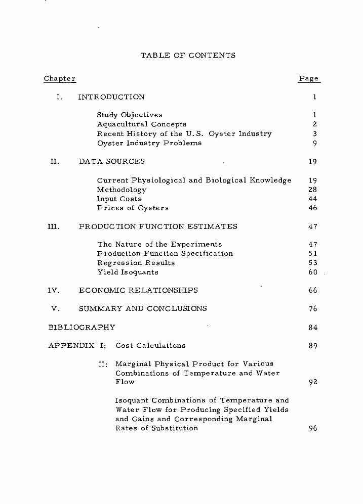
TABLE OF CONTENTS
Chapter Page
I. INTRODUCTION 1
Study Objectives 1 Aquacultural Concepts 2 Recent History of the U. S. Oyster Industry 3 Oyster Industry Problems 9
II. DATA SOURCES 19
Current Physiological and Biological Knowledge 19 Methodology 28 Input Costs 44 Prices of Oysters 46
III. PRODUCTION FUNCTION ESTIMATES 47
The Nature of the Experiments 47 Production Function Specification 51 Regression Results 53 Yield Isoquants 60
IV. ECONOMIC RELATIONSHIPS 66
V. SUMMARY AND CONCLUSIONS 76
BIBLIOGRAPHY 84
APPENDIX I: Cost Calculations 89
II: Marginal Physical Product for Various Combinations of Temperature and Water Flow 92
Isoquant Combinations of Temperature and Water Flow for Producing Specified Yields and Gains and Corresponding Marginal Rates of Substitution 96

LIST OF TABLES
Table Page
1 U.S. Oyster Prices by Regions, 1950-73 6
2 U.S. Oyster Landings by Regions, 1950-73 8
3 U.S. Canned Oyster Production and Imports, 1960-72 17
4 U. S. Fresh and Frozen Oyster Production and Imports, 1960-72 18
5 Relationship Between Salinity and Growth Rate (European flat oyster) 25
6 Effect of pH on American Oyster Pumping Activities 25
7 Temperature and Oxygen Uptake of American Oyster 27
8 Solid Wastes of American Oyster 28
9 Costs of Producing One Bushel of Oysters 37
10 Pumping Costs and Heating Costs as a Function of Water Flow 44
11 Organic Carbon Costs (in the form of algae) and Heating Costs 45
12 Current and Predicted 1976 Prices Per Gallon and Gram of Shucked Oysters 46
13 Spot Prices Per Pound and Gram of Half Shell Oysters 46
14 Newport Experiment III: October 11-December 15, 1973 Temperature-Water Flow Treatments and Average Yields in Wet Meat 47
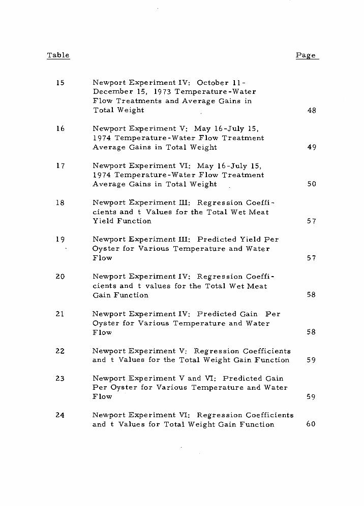
Table Page
15 Newport Experiment IV: October 11- December 15, 1973 Temperature-Water Flow Treatments and Average Gains in Total Weight 48
16 Newport Experiment V; May 16-July 15, 1974 Temperature-Water Flow Treatment Average Gains in Total Weight 49
17 Newport Experiment VI: May 16-July 15, 1974 Temperature-Water Flow Treatment Average Gains in Total Weight 50
18 Newport Experiment III: Regression Coeffi- cients and t Values for the Total Wet Meat Yield Function 5 7
19 Newport Experiment III: Predicted Yield Per Oyster for Various Temperature and Water Flow 5 7
Z0 Newport Experiment IV: Regression Coeffi- cients and t values for the Total Wet Meat Gain Function 58
21 Newport Experiment IV: Predicted Gain Per Oyster for Various Temperature and Water Flow 58
22 Newport Experiment V: Regression Coefficients and t Values for the Total Weight Gain Function 5 9
23 Newport Experiment V and VI: Predicted Gain Per Oyster for Various Temperature and Water Flow 59
24 Newport Experiment VI: Regression Coefficients and t Values for Total Weight Gain Function 60
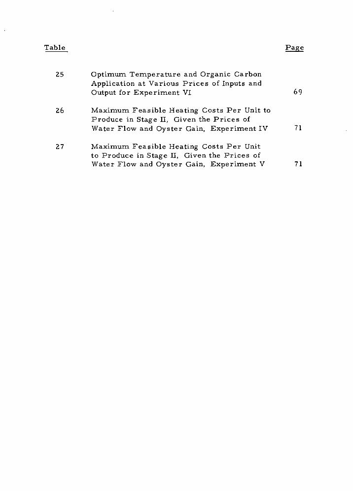
Table Page
25 Optimum Temperature and Organic Carbon Application at Various Prices of Inputs and Output for Experiment VI 69
26 Maximum Feasible Heating Costs Per Unit to Produce in Stage 11, Given the Prices of Water Flow and Oyster Gain, Experiment IV 71
27 Maximum Feasible Heating Costs Per Unit to Produce in Stage II, Given the Prices of Water Flow and Oyster Gain, Experiment V 71
LIST OF FIGURES
Figure Page
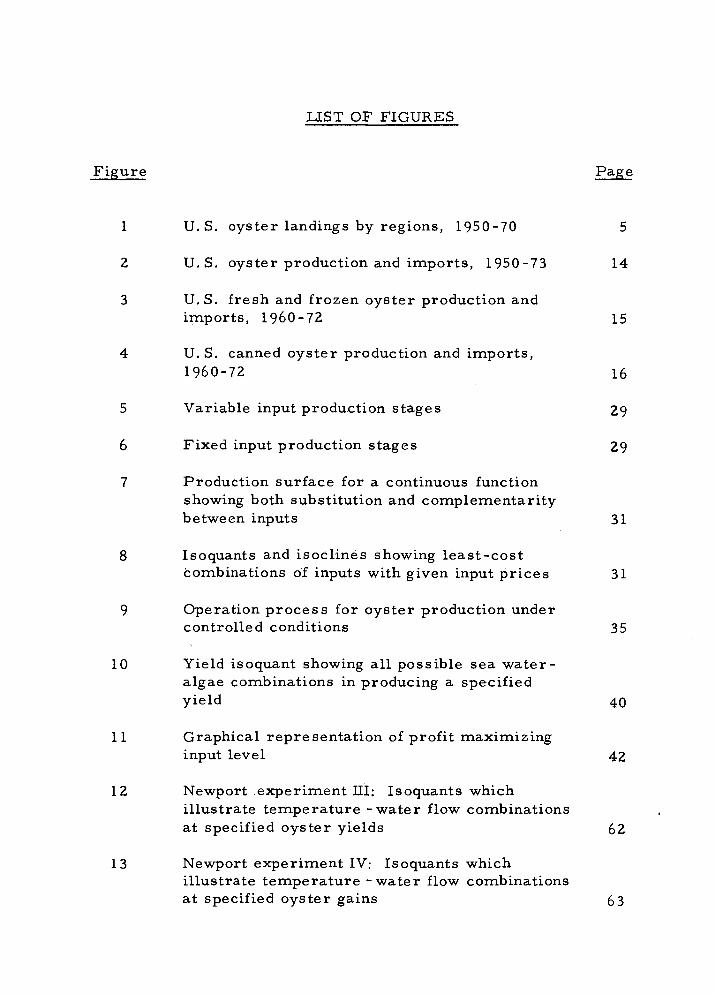
1 U.S. oyster landings by regions, 1950-70 5
2 U.S. oyster production and imports, 1950-73 14
3 U.S. fresh and frozen oyster production and imports, 1960-72 15
4 U. S. canned oyster production and imports, 1960-72 16
5 Variable input production stages 29
6 Fixed input production stages 29
7 Production surface for a continuous function showing both substitution and complementarity between inputs 31
8 Isoquants and isoclines showing least-cost combinations of inputs with given input prices 31
9 Operation process for oyster production under controlled conditions 35
10 Yield isoquant showing all possible sea water- algae combinations in producing a specified yield 40
11 Graphical representation of profit maximizing input level 42
12 Newport experiment III: Isoquants which illustrate temperature -water flow combinations at specified oyster yields 62
13 Newport experiment IV: Isoquants which illustrate temperature -water flow combinations at specified oyster gains 63
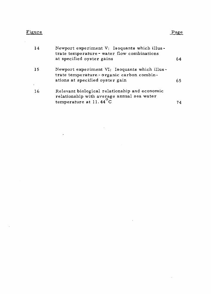
Figure Page
14 Newport experiment V: Isoquants which illus- trate temperature - water flow combinations at specified oyster gains 64
15 Newport experiment VI: Isoquants which illus- trate temperature - organic carbon combin- ations at specified oyster gain 65
16 Relevant biological relationship and economic relationship with average annual sea water temperature at 11.44 C 74

ACKNOWLEDGMENTS
The author wishes to extend appreciation to those
people who helped in the preparation of this work. The
major part of the guidance on this study came from Dr.
Frederick J. Smith,' my major professor, under whom
this project was initiated and completed. His patience
and careful guidance have been invaluable.
The author is also grateful to Mr. Robert E. Malouf,
Graduate Student in the Department of Fisheries and Wild-
life, who provided the basic biological data to this study,
to Drs. Richard S. Johnston and Richard E. Towey for their
critical review in preparation-of the mariuscripV to Dr.
William G. Brown for his statistical assistance, and to
my wife, Humi, whose encouragement made my graduate
work possible.
ECONOMIC ANALYSIS OF OYSTER PRODUCTION UNDER CONTROLLED CONDITIONS
I. INTRODUCTION
Study Obiectives
The production of oysters under natural conditions is greatly
affected by predation, disease, silting, toxins produced by plank-
tonic activities, and pollutants. However, under controlled en-
vironmental conditions, many hazardous natural and man-made
factors which adversely affect oyster growth and quality can be re-
duced or eliminated. Under controlled conditions, one can (1) in-
crease the growth rate of oysters, (2) maintain the availability of
top-quality oysters throughout the year, (3) greatly reduce the
mortality rate of oysters between the seed and the harvesting stage
of the crop, and (4) increase the volume and regularity of the supply
of oysters.
The general objective of this study is to investigate the eco:-
nomic feasibility of oyster production under controlled environment-
al conditions. Specifically, the study will:
(1) estimate biological relationships from empirical studies,
(2) determine the critical controllable variables,
(3) estimate relationships among these variables and
production, and
(4) estimate variable costs associated with these controllable
variables.
However, in order to further justify this research, the fol-
lowing topics will be also investigated;
(1) the trend of the oyster industry in North America, and
(2) the problems of the oyster industry.
Aquacultural Concepts
A definition of aquaculture is given by Ryther et al. (1968, p. 1)
i. e. , "the rearing of aquatic organisms under controlled conditions
using techniques of agriculture and animal husbandry, " Some ad-
vantages of aquaculture are well recognized: for example, con-
trollability of property rights of marine resources vis-cL-vis open
access marine resources, and the protection of the organisms from
natural and man-made disasters. However, there exist few species
of aquatic organisms which can meet whatBardach (1968, p. 6) called
"the biological properties of organisms that would lend themselves
most ideally to intensive culture. "
"(1) They should reproduce in captivity or semi-confinement or yield easily to manipulations that result in the pro- duction of their off-spring.
(2) Theireggs or larvae should be hardy and capable of being hatched or reared under controlled conditions.

(3) The food habits of larvae or young should be such that they can be satisfied by operations which can increase their natural foods or they should be able to take pre- pared foods from their early stages.
(4) They should gain •weight and nourish themselves en- tirely or in part by food items that are abundantly avail- able, that can be supplied to the organisms cheaply or that can be readily produced or increased by the people in the area where cultured species lives. "
These four criteria can not only be applied to the biological
properties of aquaculture but also give an economic limitation on
the development of aquaculture, i. e. , any difficulty in one of those
conditions will increase the cost of production.
The oyster is one of the few shellfishes that satisfies in great
degree the biological properties of aquatic organisms applicable for
aquaculture development. (1) Oysters can easily be induced to re-
produce in captivity at any time of the year, (2) oyster eggs, larvae
and seed are hardy under controlled conditions, (3) larvae and seed
can be easily reared on cultured algae, and (4) oysters can grow
and nourish themselves entirely by algae and other food sources
naturally abundant in the tide water.
Recent History of the U. S. Oyster Industry
The oyster industry of North America is comprised pri-
marily of four species. Ranked in order of commercial importance,
these are the American oyster or Eastern oyster (Crassostrea

virginica), the Pacific oyster (Crassostrea gigas), the Olympia
oyster (Ostrea lurida) and the European flat oyster (Ostrea edulis).
The American and the European flat oysters are extensively cultured
on the East Coast and the Gulf of Mexico. The Pacific and the
Olympia oysters are cultured mainly on the West Coast. But the
relative significance of the Olympia oyster has dwindled since the
importation of the Pacific oyster from Japan in the late 1910's—
Oyster production volume in the U. S. has diminished by
roughly 50 percent since the 1920's. Major declines have taken
place in such areas as Chesapeake Bay and New England. The
present production in Chesapeake Bay and New England is approxi-
mately 20 and 8 percent of their 1920 production, respectively.
The future survival of the oyster industry in the New England
region is in question (Wallace, I960). On the other hand, the
production of oysters in the Gulf of Mexico has been increasing, and
the South Atlantic and Pacific regions have maintained a constant
production level for the last two decades (Fig. 1).
During the last 20 years, ex-vessel prices of oysters have
risen from 38. 7 cents to 54. 4 cents a pound on the national average
(Table 1). As a result, the total value of the domestic landings has
— The most important cause of the phenomenon is that it takes 6-7 years for the Olympia oyster to reach market size, whereas the Pacific oyster reaches market size in 3-4 years.

Million pounds
O —O Chesapeake Bay
—D Gulf of Mexico
—% Pacific
-^ South Atlantic
Middle Atlantic New England
1950 1955 1960 1965 1970
Figure 1, U. S. oyster landings by regions, 1950-70. Source: Fishery Statistics of the U. S., U. S. D. C., 1950-70.
ui

8. (U
a,
n
a o
o
in
o
■rH
bo <u
M
<U o
0)
O
a 6 o
3 «
O 0
U
o
CD A
;
<U
fll «
u
^ «
-a § « 2
Ml
a
>-
I/JO
t^-O
OT
flOC
Mt-^
Oc
OtO
i-l^O
VO
VO
KO
OV
OO
lOO
Tfa
ilOO
O
t^
i/)>
om
inT
tiT
fro
co
co
co
mro
co
ro
to
ro
fO
ro
ro
mv
o«
3u
i
o o
\ tx
O
■* co m
TI<
t** to O
t^ t^
TH ^
CM
fM CM
»-l >H
<\J CM o^ o
a^
rl
(M >
-" C
MC
MC
MC
MC
MC
MC
O^
CO
CO
^
< <
<
• Z
2* 2
co
oo
t^
oo
t^
t^
r-c
oio
oio
oo
O'-
io
tx
Oo
oo
ow
airo
J!^
^
CO
CM
CM
CM
CM
CM
CO
CM
CM
CM
rO
CV
JC
OC
OC
MC
OrO
CO
rO
^1-
*^
^'^
"
■z z. z
cM
o\m
vo
ot^
CT
iOa
i<T
itn
uic
oc
ot^
co
'*
CO
CM
CM
CM
cO
CM
CM
CO
CM
CO
'*'<l'1
''^>
ron
'^'
O *-l CM
in >o >o < < <
z. z z
m<
'0'*
'*'*,
tfin
inin
vo
rvt^
oo
t^
t^
tv*o
io<
oio
y3'
1'^
^
' 2
2 2
co
io^
Oo
iTfio
co
o^
co
Oin
oo
oo
m
mm
mi/)in
m>
orv
o^
oo
oo
o
00 CO o o
o o
co co o
o o
to
< < <
z z z
(o
om
o^co
oo
o
CO
UIT
flO
tS
OO
OO
OO
in O O
CO O ro
to O
CO o o o
CM CM O
CO O
CO CO O
CO in o o
< <
< C
MC
MC
MC
MC
\]CM
2 2
2
o *
-icM
co
^ in
vo
t^
oo
o^
o r
HC
McO
Tt^
invo
t^o
oa^
o I-<
CM
CO
in
inin
inin
inin
intn
inio
^o
iov
ov
o^
o >
o'v
o ko «
t^ r^
t^
t^
CO
o
in
<7\

risen slightly. However, the regional variations in price are
rather significant. In the Middle Atlantic states ex-vessel prices
have risen from 36 cents per pound in 1950 to $1. 30 per pound in
1970. The price per pound of oysters in New England has increased
from 52 cents in 1950 to $2. 00 in 1970. The total value of produc-
tion in the Middle Atlantic states has decreased significantly from
9-6 million dollars in 1950 to 1.8 million dollars in 1970 in spite
of a surge in price and, in the New England region, the value of
production has declined from 1. 7 million dollars to 0.4 million
dollars over the same period.
Oyster production in the Chesapeake Bay and South Atlantic
regions has declined slightly over the last two decades. Production
has decreased in Chesapeake Bay from 30 million pounds in 195 0
to 24. 7 million pounds in 1970. However, the value of production
has increased from 11. 1 million dollars to 15. 1 million dollars
during the same period.
Oyster production of the Pacific region has been rather stable
for the last 20 years. The production has not changed much in
volume, while 1970 oyster prices have increased about 70 percent
from 1950. The Gulf Coast is the only region where total production
as well as total value has increased in the last two decades (Table 2).
There are several price elasticities of demand for oysters.
The Gulf Coast produces, mostly, shucked oysters where an

Table 2. U. S. Oyster Landings by Regions, 1950-73 millions of pounds (meat weight) and millions of dollars
Year New ! England Middle Chesapeake South Gulf Pacific Total dom.
T Total 1 Imports as
Atlantic Bay Atlantic Coast Coast landi ines imporus
supply a 1 % of
Qty. Value Qty. Value Qty. Value Qty. Value Qty. ' Value Qty. Value Qty. ' Value Qty. Value Qty. Value total yalue
1950 .4.7 1.7 18.2 9.6 30.0 11-1 3.0 1.0 .12.3 4.0 8.2 2.2 76.4 29.6 0.4 0.3 76.8 29.9 1.0
1951 2.0 1.0 17.4 9.7 29.6 12.0 3.8 1.2 11.6 3.2 8.7 2.0 73.0 29. 1 1.0 0.5 74.0 29.6 1.7
1952 2.2 1.0 16.8 9.1 34.4 14.9 4. 1 1.2 14.6 4.0 10. 1 2.0 82.2 32.3 0.6 0.4 82.9 32.7 1.2
1953 1.0 .6 14.5 7.3 26.9 14.7 4.0 1.0 12.8 3.6 10.4 1.8 79.7 29. 1 0.7 0.4 80.4 27.3 1.4
1954 .7 .5 13.4 7.5 41.6 18.9 3.8 1.0 11.4 3.1 11.0 1.9 81.9 32.8 1. 1 0.6 83.1 33.4 1.8
1955 .6 .5 9.8 5.3 39.2 17.8 2.3 0.7 13.9 3.7 11.7 2.5 77.5 30.5 1.5 0.7 79.0 31. 1 2.3
1956 .5 .4 8.5 4.2 37.1 18.7 3.7 1.0 13.5 3. 1 11.9 2.8 75.1 30.8 1.9 0.8 77.1 31.7 2.5
1957 .4 .4 8.0 5.0 34.2 17.2 3. 1 0.9 14.3 3.7 11.7 2.2 71.7 29.4 2.7 1.0 74.3 30.4 3.3
1958 .3 .3 4.3 3.4 37.5 20.8 2.7 0.8 10.4 3.0 11.2 2.2 66.4 30.4 5.4 1.6 71.8 32.0 5.0
1959 .4 .5 . 1. 4 1.3 33.3 20.6 3.5 1.0 13.7 3.8 12.4 2.3 64.7 29.5 6.0 2.0 70.6 31.4 6.4
1960 .5 .6 .1.2 1.2 27. 1 19.3 4.1 1.6 16.1 4.3 11.0 2.3 60.0 29.2 7.0 2.3 67.0 31.5 7.3
1961 .5 .5 1.9 2.0 27.5 21.7 4.0 1.8 18.2 5. 1 10.2 2.0 62.3 33.2 7.7 2.4 70.0 35.6 6.7
1962 .3 .4 2.4 2.6 19.9 16.0 3.8 1.7 18.8 5.9 10.8 2.6 56.0 29. 1 7.8 2.8 63.9 31.9 8.8
1963 .5 .5 .1.0 1.0 18.3 13.7 4.8 2.0 24.1 7.2 9.8 2.5 53.4 27.1 8.5 3.1 66.9 36.2 10.3 1964 .2 .3 .1.4 1.4 22.1 15.8 3.5 1.5 23.4 6.3 10.0 2.6 60.5 27.9 8.0 2.9 68.5 30.8 9.4
1965 .3 .7 ..8 1.1 21.2 16.7 4.1 1.5 19.2- 5.7 9.2 2.2 54.7 27.9 8.6 3.2 63.3 31.1 10.3
1966 .4 .8 ..9 1.2 21.2 14.5 3.7 1.6 17.2 6.5 7.8 2.7 51.2 27.4 12.0 4.5 63.2 31.9 14. 1 1967 .3 .7 -1.2 1.2 25.4 17.1 3.2 1.4 21.2 8.0 8.8 3.9 50.0 32.2 16.1 5.8 76.1 38. 1 18.0
1968 .2 .5 .1.5 1.5 22.2 14.9 3.0 1.5 26.7 10.3 7.8 3.0 61.9 32.0 14.5 5.6 76.4 37.7 14.9 1969 .2 .4 1.3 1.3 22.2 14.0 1.8 1.1 19.8 8.1 7.0 2.6 52.2 27.5 16.7 6.4 68.9 33.9 18.8 1970 .2 .4 1.4 1.8 24.7 15.1 1.6 1.0 17.7 7.5 8.0 3.7 53.6 29.5 15.0 8. 1 68.6 37.6 21.5
1971 N.A. N.A. N.A. N.A. N.A. N;A. N.A. N.A. N.A. N.A. N.A. N.A. 54.6 30.4 9.5 6.7 64.0 37.0 18.1
1972 N.A. N.A. N.A. N.A. N.A. N.A. N.A. N.A. N.A. N.A. N.A. N.A. 52.5 33.8 20.8 13.8 73.4 43.6 27.8
1973 N.A. N.A. N.A. N.A. N.A. N.A. N.A. N.A. N.A. N.A. N.A. N.A. 48.6 35.2 1979 11.6 68.5 46.3 24.8
Source: Fishery Statistics of the U. S., U. S. D. C., 1950-73.
00

increase in oyster production has been accompanied by a more than
proportionate increase in total receipts. On the other hand, the
Pacific region and the domestic aggregate supply have not only de-
creased but also their total receipts have increased over the two
decades (Table 2). However, caution should be exercised in the
interpretation of the price elasticities of demand. Each product
such as shucked, half-shell, or smoked oysters may show a different
price elasticity of demand. .
Oyster Industry Problems
The problems dealt with in this section may be specific to a
particular region in the U.S. or applicable to the entire U.S. oyster
industry. These problems (Wallace, I960; Engle, 1966; Windham,
1968; Matthiessen, 1970; Sokoloski, 1970; Bardach et al. , 1972) are
as follows:
(1) The supply of oyster seed; Oyster seed, in most areas,
depends entirely upon natural settings, and is greatly affected by
2/ environmental factors.— The natural settings in some areas like
New England, Middle Atlantic and Chesapeake Bay have not been
favorable because of the lack of sufficient numbers of mature oysters
2/ — The Pacific oyster industry is heavily dependent upon imports of oyster seed from Japan.
10
to produce enough seed for the industry. Yet, oyster seed hatch-
eries have not shown the capacity to supply more seed to the indus-
try. Perhaps oyster seed hatcheries have such potential, but un-
certainties in natural settings are likely to be an impediment to the
establishment of hatcheries, since good natural settings would
probably bring a far lower price for seed than for the product of
hatcheries.
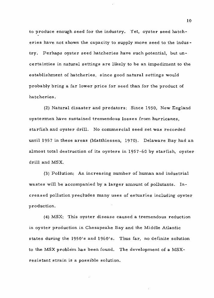
(2) Natural disaster and predators: Since 1950, New England
oystermen have sustained tremendous losses from hurricanes,
starfish and oyster drill. No commercial seed set was recorded
until 1957 in these areas (Matthiessen, 1970). Delaware Bay had an
almost total destruction of its oysters in 1957-60 by starfish, oyster
drill and MSX.
(3) Pollution: An increasing number of human and industrial
wastes will be accompanied by a larger amount of pollutants. In-
creased pollution precludes many uses of estuaries including oyster
production.
(4) MSX: This oyster disease caused a tremendous reduction
in oyster production in Chesapeake Bay and the Middle Atlantic
states during the 1950's and 1960's. Thus far, no definite solution
to the MSX problem has been found. The development of a MSX-
resistant strain is a possible solution.

11
(5) Technology: There has been little technological change
in harvesting and distribution. In some areas, a reduction in the
scale of operation due to a decrease in oyster production by disease
and hurricanes has forced the use of (less efficient) tongs instead of
dredges. However, a considerable breakthrough in productivity
could have a substantial effect on the industry.
(6) Regulatory structure: Present regulations concerning the
use of state and local estuaries have emerged over the past several
decades, and the conditions for the lease of common property for
private use have become extremely stringent in some areas such as
New England. Matthiessen states (1970, p. 10) that:
"In States such as Rhode Island and Massachusetts, it is exceedingly difficult to obtain exclusive fishing rights to areas of coastal water. Legislation regarding private lease is restrictive, and there are increasing conflicts between commercial and recreational interests. "
(7) Competition for resources: Changes in technology, popu-
lation and social values have brought new competition for the use of
common properties. The majority of the oyster beds in the U.S.
are public grounds (Bardach, 1968, p. 1). Oyster growers must
compete with nonfishery uses of the resource base. As social
opportunity costs for public property becomes higher, the public
authorities become reluctant to lease the common property for a
low rent.

12
(8) Consumption patterns: It seems that there has been a
gradual change in the U.S. consumers' tastes toward less con-
sumption of oysters (Sokoloski, 1970, p. 4). The incoine elasticity
of demand for oysters has been estimated at 0. 25 (Bell, 1969, P- 7),
i. e. , the consumption of oysters is less than proportional to income
3/ increase.- New marketing and distribution changes, and perhaps
new product forms could reverse this relationship.
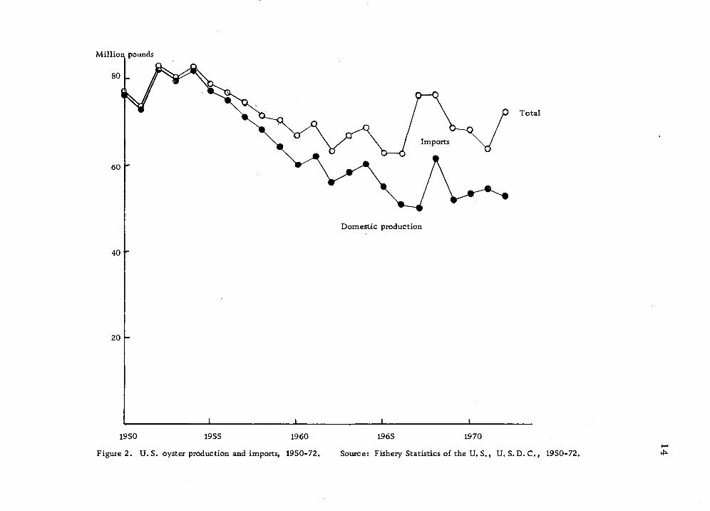
(9) Role of imports: Imports of oyster products in the U. S.
market have increased from 5. 8 million pounds, valued at 0. 6
million dollars in 1950, to 19. 9 million pounds valued at 11.6 million
dollars in 1973. The total market share of imports surged from
1. 0 percent to 24.8 percent in the same period (Table 2). Oyster
imports consist of four major items: fresh and frozen, canned,
seed, and oyster juice (U.S.D. C. , 1973). Canned items such as
smoked and cooked oysters constituted 97 percent of the imported
value in 1972. In that year half of the canned items were consumed
in the Pacific region. The major suppliers of these products in
1972, in order of importance, were Japan, Korea, and Hong Kong.
Prices of imports have been considerably lower than the average
3/ — This statement may be misleading in the sense that a lumped estimate does not reflect the true estimate of each product.
13
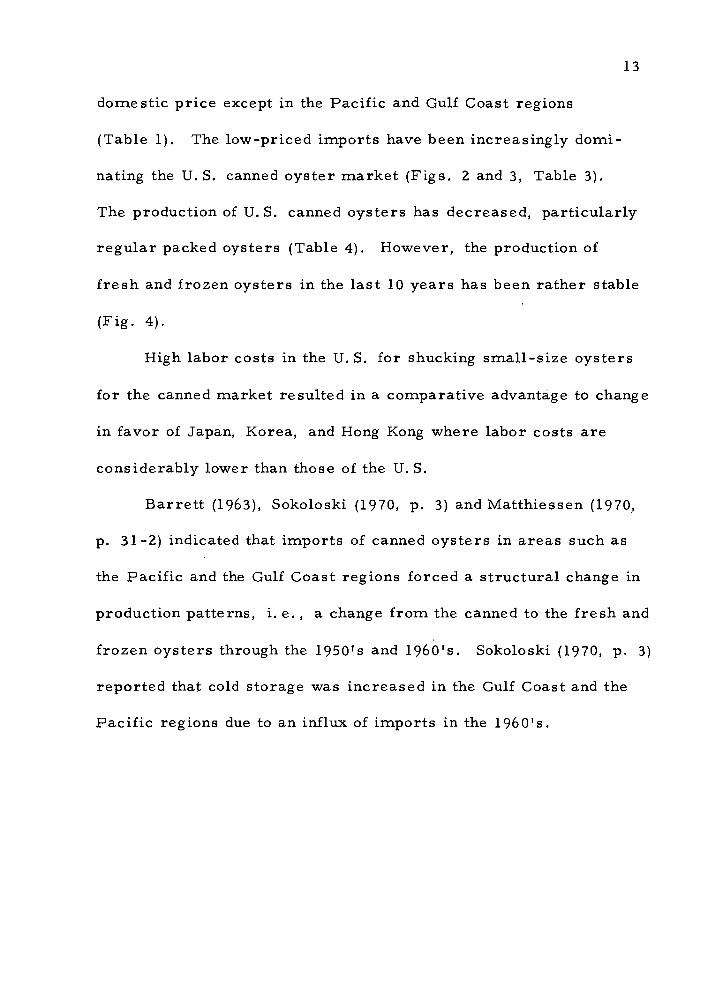
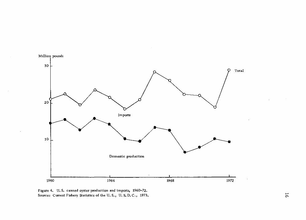
domestic price except in the Pacific and Gulf Coast regions
(Table 1). The low-priced imports have been increasingly domi-
nating the U.S. canned oyster market (Figs. 2 and 3, Table 3).
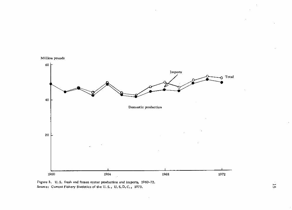
The production of U. S. canned oysters has decreased, particularly
regular packed oysters (Table 4). However, the production of
fresh and frozen oysters in the last 10 years has been rather stable
(Fig. 4).
High labor costs in the U. S. for shucking small-size oysters
for the canned market resulted in a comparative advantage to change
in favor of Japan, Korea, and Hong Kong where labor costs are
considerably lower than those of the U.S.
Barrett (1963), Sokoloski (1970, p. 3) and Matthiessen (1970,
p. 31-2) indicated that imports of canned oysters in areas such as
the Pacific and the Gulf Coast regions forced a structural change in
production patterns, i. e. , a change from the canned to the fresh and
frozen oysters through the igSO's and igSO's. Sokoloski (1970, p. 3)
reported that cold storage was increased in the Gulf Coast and the
Pacific regions due to an influx of imports in the 1960's.
40 -
20 -
Total
Domestic production
J_ -l_
1950 1955 1960
Figure 2. U.S. oyster production and imports, 1950-72.
1965 1970
Source: Fishery Statistics of the U. S., U. S.D. C, 1950-72. ^
Million pounds
60
20
Imports Total
Domestic production
1960 1964 1968 1972
Figure 3. U, S. fresh and frozen oyster production and imports, 1960-72. Sources Current Fishery Statistics of the U. S., U. S0D. C., 1973. ui
Total
1960 1964 1968 1972
Figure 4. U. S. canned oyster production and imports, 1960-72. Source: Current Fishery Statistics of the U. S., U. S. D. C., 1973. O

Table 3. U. S. Canned Oyster Production and Imports, 1960-72 (millions of pounds) _a/
Year Pack Total
Canned imports
Total Regular
Smoked Stews Bisque and
soup supply
East and Gulf West Coast
1960 8.8 3.8 0.2 1.7 £/ 14.5 6.5 21.0 1961 10.6 2.6 0.1 1.9 c/ 14.3 7.2 22.5 1962 6.8 3.0 0.2 2.2 s/ 12.3 7.3 19.5 1963 10.4 2.9 0. 1 2.4 £/ 15.8 7.9 23.7 1964 10.1 2.4 0.1 1.6 £/ 14.2 7.4 21.6 1965 8.1 b/ 0.1 2.1 £/ 10.3 8.0 18.8 1966 5.8 b/ 0.1 3.9 £/ 9.8 11.2 21.0 1967 9.8 b/ 0.1 3.4 £/ 13.3 15.0 28.2 1968 9.5 b/ 1.4 2.8 £/ 12.6 13.5 26. 1 1969 4.2 b/ 0.0 2.2 0.2 6.6 15.6 22. 1 1970 4. 1 b/ 0.1 3.7 0.1 8.0 13.9 21.9
1971 7.2 b/ 0.1 2.9 £/ 10.2 8.8 18.9 1972 5.9 b/ 0.1 3.6 £/ 9.5 13.4 28.9
^/ Meat weight b/ West Coast included with East Coast and Gulf cl Less than 0. 05 million pounds
Source: Current Fishery Statistics of the U. S., U.S.D.C, 1973
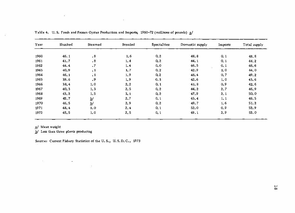
Table 4. U. S. Fresh and Frozen Oyster Production and Imports, 1960-72 (millions of pounds) ±1
Year Shucked Steamed Breaded Specialties Domestic supply Imports Total supply
1960 46.1 .8 1.6 0.2 48.8 0.1 48.8 1961 41.7 .8 1.4 0.2 44. 1 0. 1 44.2 1962 44.4 .7 1.4 0.0 46.5 0. 1 46.6 1963 40.9 . 1 1.7 0.2 42.9 1.0 44.0 1964 46.1 .1 1.9 0.2 48.4 0.7 49.2 1965 39.6 .9 1.9 0.3 42.6 1.0 43.6 1966 38.4 1.0 2.2 0.1 41.8 0.9 42.6 1967 40.3 1.3 2.5 0.2 44.2 2.7 46.9 1968 43.2 1.5 3.1 0.2 47.9 2. 1 50.0 1969 42.7 b/ 2.7 0.1 45.4 1. 1 46.5 1970 46.5 b/ 2.9 0.2 49.7 1.6 51.2 1971 48.4 1.0 2.4 0.1 52.0 0.9 52.9 1972 45.5 1.0 2.5 0.1 49. 1 2.9 52.0
a/ Meat weight hj Less than three plants producing
Source: Current Fishery Statistics of the U. S., U. S. D. C, 1973
00
19
II. DATA SOURCES
The data used for the economic analysis in this study were
obtained from secondary sources, particularly from experiments
conducted by the Department of Fisheries and Wildlife, Oregon State
University, from 1973 to 1974 at Newport, Oregon. These experi-
ments were intended (1) to examine the effect on salmon and oyster
production of effluent from a possible nuclear power plant on the
Pacific Northwest, (2) to investigate season changes in oyster growth
patterns due to a change in natural food supply, and (3) to identify
what constitutes the biologically optimum water flow and temperature
for oysters without artificial feeding.
Some physiological research of the Pacific oyster lacks neces-
sary information for economic analysis (e.g., specifications of
critical variables). This information was supplemented by data for
other species of oysters, e.g. , American and European oysters.
Current Physiological and Biological Knowledge
The Pacific oyster, Crassostrea gigas (Thunberg) is native to
Japan from which it was imported in the late ^lO's. It is widely
cultivated on the West Coast of the U. S. and Canada as well as in
Japan. Although the Pacific oyster has acclimatized to a new en-
vironment, only a few places in Washington and British Columbia

20
have sufficiently high enough water temperatures to permit repro-
duction.
Under natural conditions on the West Coast of the United
States and Canada, the life cycle of the Pacific oyster starts in
June with spawning of the eggs by the female and the fertilization
of those eggs by the male. After 24 hours or so the eggs hatch into
free-swimming larvae. About three weeks later the larvae attach
themselves to a smooth hard surface. Thereafter, the oysters
grow rapidly until the water temperature reaches 22 to 23 C.
The growth of the oysters is suspended twice a year, once due to
spawning activities, and the other due to hibernation. These be-
havioral changes are caused by changes in environmental temper-
ature.
Growth
Many different criteria have been used to measure the growth
of oysters. As a basic criterion for growth measurement, biologists
tend to use shell length. However, the growth of oysters is most
accurately measured by (1) the condition index (the condition index
refers to the ratio of the dry meat weight to the 'interior' shell
volume times 1, 000), or (2) (a better measure of growth) the total
energy content of the body (Warren and Davis, 1967)

21
of oyster is apparently most advantageous. However, there are
some serious difficulties when the oysters must be measured on a
continuous basis in a controlled population.
In general, growth rates of oysters vary with size and age.
The growth rates of oysters decrease as oysters increase in size,
since an increase in total weight would require more energy to
maintain their bodies.
Environmental Factors
Oyster growth is interrelated with many known and unknown
environmental factors. Variations in growth rate among the same
species are evidenced by the existence of different physiological
races of oysters. However, many biologists agree that temperature,
food supply, salinity, pH and dissolved oxygen in sea water play a
major role in the growth rate of oysters (Pereyra, 1962; Chew,
1963; Matthiessen and Toner, 1966; Glaus and Alder, 1970). En-
vironmental factors identified from literature reviews are as follows:
(1) Temperature of water ( C)
(2) Salinity (ppt)
4/ (3) pH -'
4/ — The term pH is used to indicate the degree of acidity of a
solution by measuring the quantity of free hydrogen ions (H ).

22
(4) Food supply (organic carbon or equivalent cell number/ oyster/minute)
(5) Water supply (milliliters/ oyster/minute)
(6) Dissolved oxygen, 0 (micromilliliters/oyster/minute)
(7) Oyster wastes
The parameters that affect oyster growth play a different role
among the physiological races. In order to see the contribution of
each parameter, it is desirable to use controlled environments.
However, it is extremely difficult to evaluate the complexity of bio-
chemical interactions that can occur, and to measure the ability of
shellfish to improvise when the quantity of a particular substance is
low or zero. Little information is available to substantiate the de-
tailed analysis of interactions.
Temperature in Relation to Growth
The relationship between growth and water temperature has
been the subject of numerous studies on fishes as well as on shell-
fishes. Biologists have been successful in describing major tem-
perature effects on behavior and rates of various biochemical
processes. Temperature plays an important role in physiological
activities, and ultimately in the biochemical reactions of animals.
It regulates rate of digestion and consequently maximum daily food
consumption.
23
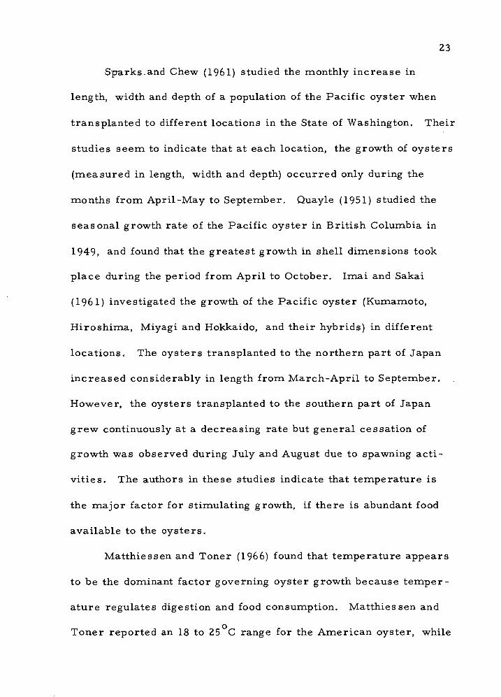
Sparks.and Chew (I96I) studied the monthly increase in
length, width and depth of a population of the Pacific oyster when
transplanted to different locations in the State of Washington. Their
studies seem to indicate that at each location, the growth of oysters
(measured in length, width and depth) occurred only during the
months from April-May to September. Quayle (1951) studied the
seasonal growth rate of the Pacific oyster in British Columbia in
1949, and found that the greatest growth in shell dimensions took
place during the period from April to October. Imai and Sakai
(1961) investigated the growth of the Pacific oyster (Kumamoto,
Hiroshima, Miyagi and Hokkaido, and their hybrids) in different
locations. The oysters transplanted to the northern part of Japan
increased considerably in length from March-April to September.
However, the oysters transplanted to the southern part of Japan
grew continuously at a decreasing rate but general cessation of
growth was observed during July and August due to spawning acti-
vities. The authors in these studies indicate that temperature is
the major factor for stimulating growth, if there is abundant food
available to the oysters.
Matthiessen and Toner (1966) found that temperature appears
to be the dominant factor governing oyster growth because temper-
ature regulates digestion and food consumption. Matthiessen and
Toner reported an 18 to 25 C range for the American oyster, while
24
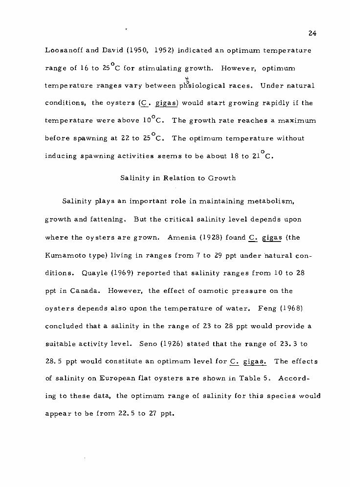
Loosanoff and David (1950, 195 2) indicated an optimum temperature
range of 16 to 25 C for stimulating growth. However, optimum
temperature ranges vary between phsiological races. Under natural
conditions, the oysters (C . gigas) would start growing rapidly if the
temperature were above 10 C. The growth rate reaches a maximum
o before spawning at 22 to 25 C. The optimum temperature without
o inducing spawning activities seems to be about 18 to 21 C.
Salinity in Relation to Growth
Salinity plays an important role in maintaining metabolism,
growth and fattening. But the critical salinity level depends upon
where the oysters are grown. Amenia (1928) found C^ gigas (the
Kumamoto type) living in ranges from 7 to 29 ppt under natural con-
ditions. Quayle (1969) reported that salinity ranges from 10 to 28
ppt in Canada. However, the effect of osmotic pressure on the
oysters depends also upon the temperature of water. Feng (1968)
concluded that a salinity in the range of 23 to 28 ppt would provide a
suitable activity level. Seno (1926) stated that the range of 23. 3 to
28. 5 ppt would constitute an optimum level for C^ gigas. The effects
of salinity on European flat oysters are shown in Table 5. Accord-
ing to these data, the optimum range of salinity for this species would
appear to be from 22. 5 to 27 ppt.

25
Table 5. Relationship Between Salinity and Growth Rate (European Flat Oyster)
Salinity (ppt) Growth (Micron) in 10 days
27 252 25 250 22.5 247 20 223 17.5 210 15.0 190
Source: Davis etal., 1962
pH in Relation to Growth
Apparently changes in pH value affect pumping activities and
oxygen uptake (Goftsoff, 1964). Table 6 indicates that normal
pumping occurs at a pH level of 7. 75, whereas at pH levels below
7. 00 the pumping rate is reduced. Loosanoff and Tommers (1947)
reported that the oyster's rate of pumping is affected by pH value,
and suggested that a pH range of 7. 5 to 8. 2 would constitute an
optimum value for adult oysters.
Table 6. Effect of pH on Pumping Activities of the American Oyster
pH Remarks
7. 75 Normal pumping 6. 75-7. 00 Vigorous pumping for several hours and then
reduction 6.50 Decrease in pumping, and shell opens for less time 4. 25 10 percent of normal pumping
Source: Galtsoff, 1964
26
Food in Relation to Growth
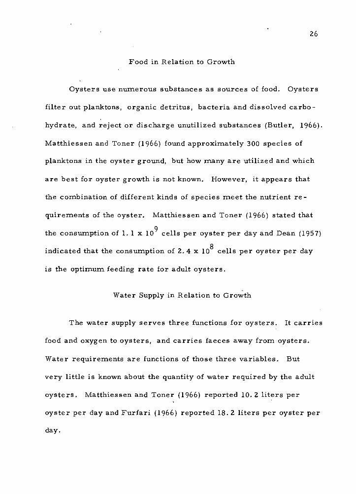
Oysters use numerous substances as sources of food. Oysters
filter out planktons, organic detritus, bacteria and dissolved carbo-
hydrate, and reject or discharge unutilized substances (Butler, 1966).
Matthiessen and Toner (I966) found approximately 300 species of
planktons in the oyster ground, but how many are utilized and which
are best for oyster growth is not known. However, it appears that
the combination of different kinds of species meet the nutrient re-
quirements of the oyster. Matthiessen and Toner (1966) stated that
9 the consumption of 1. 1 x 10 cells per oyster per day and Dean (1957)
Q
indicated that the consumption of 2. 4 x 10 cells per oyster per day
is the optimum feeding rate for adult oysters.
Water Supply in Relation to Growth
The water supply serves three functions for oysters. It carries
food and oxygen to oysters, and carries faeces away from oysters.
Water requirements are functions of those three variables. But
very little is known about the quantity of water required by the adult
oysters. Matthiessen and Toner (I966) reported 10.2 liters per
oyster per day and Furfari (I966) reported 18. 2 liters per oyster per
day.
27
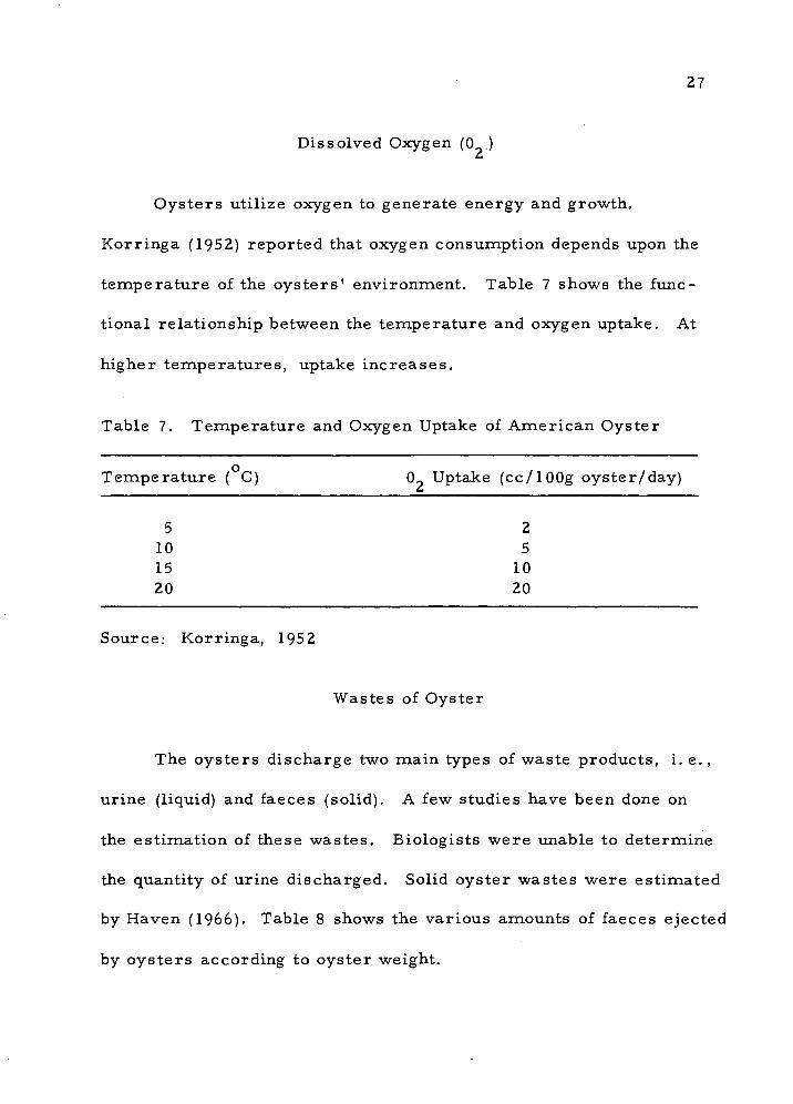
Dissolved Oxygen (0 )
Oysters utilize oxygen to generate energy and growth.
Korringa (1952) reported that oxygen consumption depends upon the
temperature of the oysters' environment. Table 7 shows the func-
tional relationship between the temperature and oxygen uptake. At
higher temperatures, uptake increases.
Table 7. Temperature and Oxygen Uptake of American Oyster
Temperature ( C) 0 Uptake (cc/lOOg oyster/day)
5 2 10 5 15 10 20 20
Source: Korringa, 1952
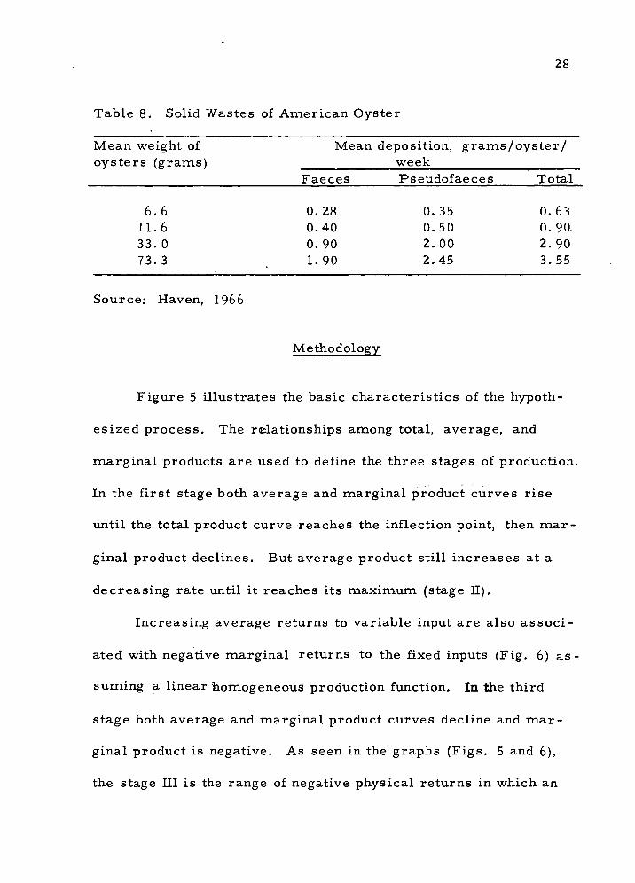
Wastes of Oyster
The oysters discharge two main types of waste products, i. e. ,
urine (liquid) and faeces (solid). A few studies have been done on
the estimation of these wastes. Biologists were unable to determine
the quantity of urine discharged. Solid oyster wastes were estimated
by Haven (1966). Table 8 shows the various amounts of faeces ejected
by oysters according to oyster weight.
28
Table 8. Solid Wastes of American Oyster
Mean weight of oysters (grams)
Mean deposition, grams /oyster/ week
Faeces Pseudofaeces Total
6.6 11.6 33. 0 73.3
0. 28 0.40 0. 90 1. 90
0.35 0.50 2.00 2.45
0.63 0. 90. 2.90 3.55
Source: Haven, 1966
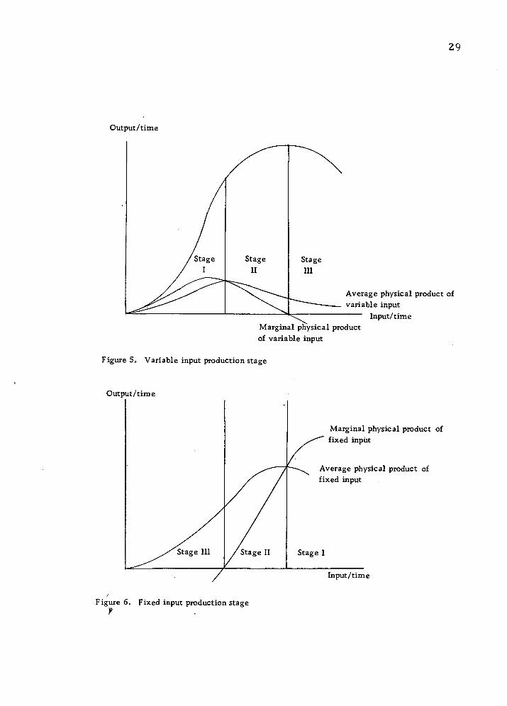
Methodology
Figure 5 illustrates the basic characteristics of the hypoth-
esized process. The relationships among total, average, and
marginal products are used to define the three stages of production.
In the first stage both average and marginal product curves rise
until the total product curve reaches the inflection point, then mar-
ginal product declines. But average product still increases at a
decreasing rate until it reaches its maximum (stage II).
Increasing average returns to variable input are also associ-
ated with negative marginal returns to the fixed inputs (Fig. 6) as-
suming a linear homogeneous production function. In the third
stage both average and marginal product curves decline and mar-
ginal product is negative. As seen in the graphs (Figs. 5 and 6),
the stage III is the range of negative physical returns in which an
29
Output/time
Average physical product of variable input
Input/time Marginal physical product of variable input
Figure 5. Variable input production stage
Output/time
Marginal physical product of fixed input
Average physical product of fixed input
Stage I
Input/time
Figure 6. Fixed input production stage

30
additional input is associated with a decreasing total product. It
is obvious that production should not be carried out in this region,
unless the input has a negative cost or subsidy.
The previous section explained the one input and one output
production situation. But a realistic consideration of production
relationships is generally given only by several inputs and one or
more outputs. Selection of the least-cost combination requires
information regarding the production function, isoquants, and
relative input prices. Ferguson (1972, p. 138) defines the pro-
duction function as such;
"A production function is a schedule (or table, or mathematical equation) showing the maximum amount of output that can be produced from any specified set of inputs, given the existing technology or 'state of art. ' In short run, the production function is a catalogue of output possibilities. "
Assuming a continuous production relationship, a general
production surface is shown in Figure 7. From the equation de-
rived from the production relationships, the isoquant will be given.
Ferguson (1972, p. 172) goes on defining the isoquant as such:
"An isoquant is a curve in input space showing all possible combination of inputs physically capable of producing a given level of output . . . . "
The isoquant is shown by dropping perpendiculars from the
same level of outputs onto the production surface to the input plane
(i. e. , ABC in Fig. 7).

31
Output/time
1st input/time 2nd input/time
Figure 7. Production surface for a continuous production function showing both substitution and complementarity between inputs
Isocline (equal price ratio: between inputs)
Isoquant Isocost
2nd input/time
Figure 8. Isoquants and isoclines showing least-cost combinations of inputs with given input prices
32
Optimum Combinations of Input
The isoquant only tells us various combinations of inputs that
produce a constant output. In deriving an optimum input level for
that isoquant, the relative prices of inputs must be introduced.
Given isoquants, a least-cost combination of factor inputs can be
found at the point where the marginal rates of substitution are equal
to the inverse of input price; ratio, then the various loci of least-cost
combinations of inputs when input prices remain constant are called
the expansion path.
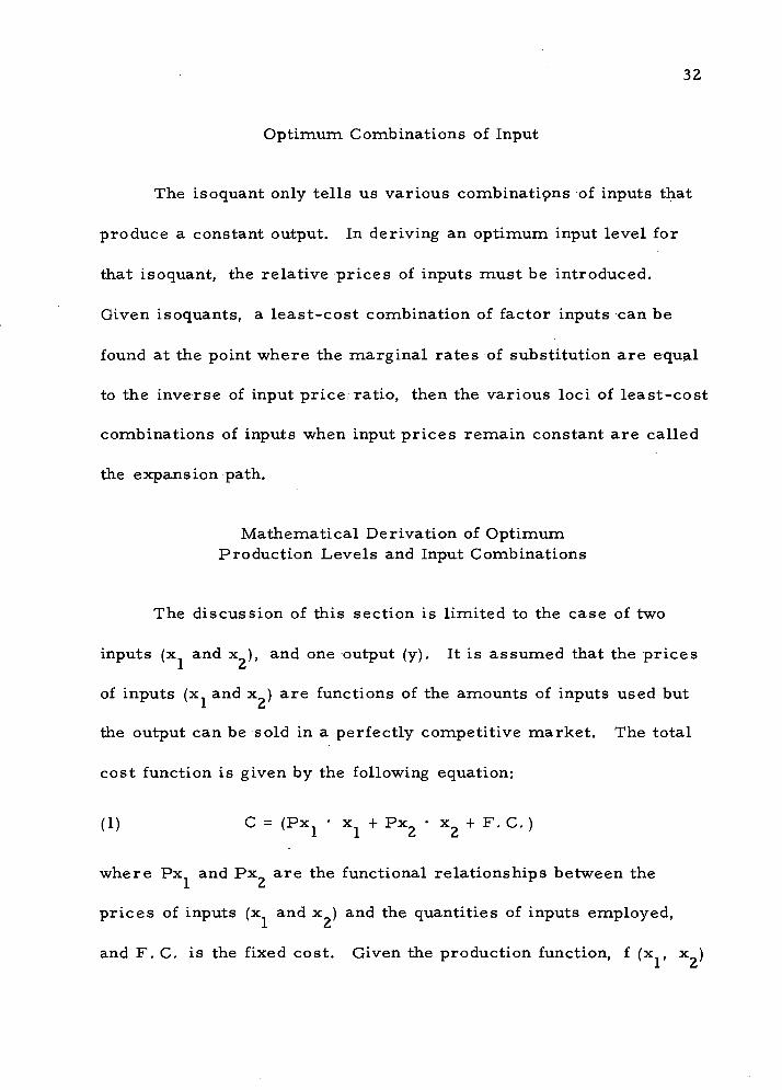
Mathematical Derivation of Optimum Production Levels and Input Combinations
The discussion of this section is limited to the case of two
inputs (x and x ), and one output (y). It is assumed that the prices
of inputs (x and x ) are functions of the amounts of inputs used but
the output can be sold in a perfectly competitive market. The total
cost function is given by the following equation:
(1) C = (Px ' x + Px2 • x2 + F. C. )
where Px and Px are the functional relationships between the
prices of inputs (x and x ) and the quantities of inputs employed, X c*
and F. C. is the fixed cost. Given the production function, f (x , x )
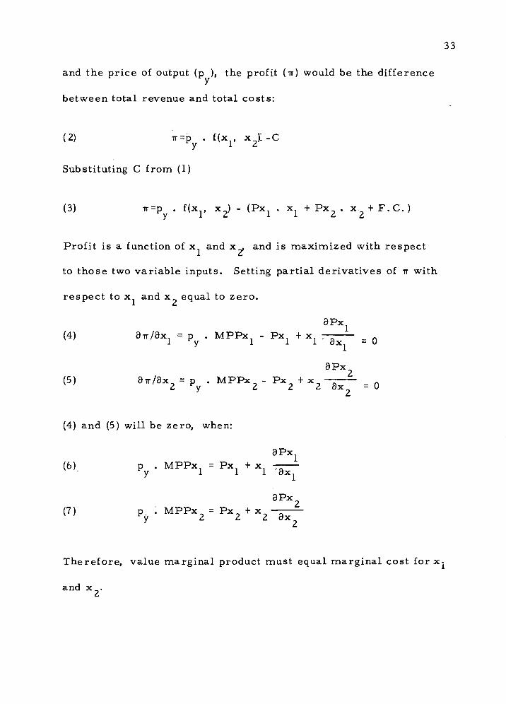
33
and the price of output (p ), the profit (TT) would be the difference
between total revenue and total costs:
(2) iT=p . f(x , xt-C y 1 Z
Substituting C from (1)
(3) iT=p . f(x xj - (Px . x + Px . x + F. C. ) y 1 Z 1 i c. 2
Profit is a function of x and x^ and is maximized with respect
to those two variable inputs. Setting partial derivatives of TT with
respect to x and x equal to zero.
aPx (4) aWax. = p . MPPx - Px. + x. rr _ n 1 y 1 11 ax. - u
aPx (5) awax2 = py . MPPX2 - PX2 + x2— = 0
(4) and (5) will be zero, when:
aPx (6) p . MPPx = Px + x —
y 111 ax.
apx (7) p, I MPPx = Px, + x.
y 2 2 2 ax.
Therefore, value marginal product must equal marginal cost for x.
and x .

34
This tells us that for profit maximization, each input should be
utilized up to the point where value of the marginal product is equal
to the marginal input cost.
Oyster Production
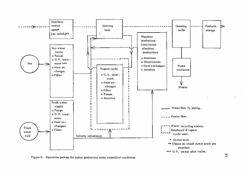
Figure 9 shows the basic operations of oyster culture under
controlled environmental conditions. Mathiessen and Toner (1966)
American Cyanamid Company (1968, Volume 2) reported detailed
engineering studies on algae and oyster production. They listed
the following as major fixed factors for algae and oyster produc-
tion:
Algae culture (continuous culture)
(1) Illumination (2) Air compressors (3) Delivery systems (4) Structures (5) Tanks (6) Pipings (7) Heat exchangers
Oyster growing tanks
(1) Baskets (2) Tanks (3) Pumps (4) Pipings (5) Heat exchangers (6) Structures (7) Filtration systems
The American Cyanamid Company reports have come up with_a
cost calculation on the basis of producing 100, 000 bushels of
Hatchery reared
spats* (no cultch)**
Sea water intake
o Pumps o U.V. treat-
ment *** o Heat ex-
changer o Filter
Fresh water supply
o Pumps o U.V. treat-
ment o Heat ex-
changers o Filter
<-
A
\./
Growing tank
V
Repeat cycle
o U.V. treat- ment
o Heat ex- changer
o Filter o Pumps o Aeration
Plankton production (continuous plankton production)
o Nutrients o Illumination o Heat exchanger o Aeration
A
'IK Salinity adjustment
Dressing
table
Waste treatment
V Wastes
Water flow by piping.
. _ Oyster flow.
r 1 Water recycling system.
I ! Employed if repeat
cycle used.
* Oyster seed. ** Object on which oyster seeds are
attached. *** U.V. means ultra violet.
Figure 9, Operation process for oyster production under controlled conditions Ui
36
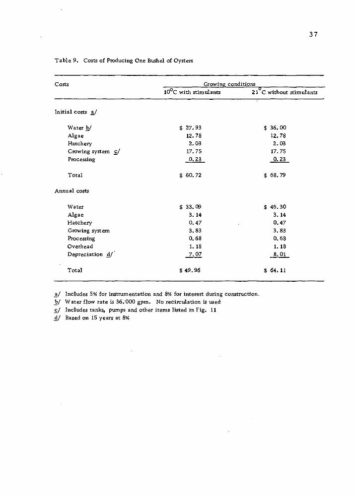
oysters per year. Table 9 shows the results of this study.
Table 9 indicates that major costs of producing oysters under
controlled environmental conditions are water, algae and growing
system. However, the relative significance of water costs, which
include the heating of water, are greater than the costs of the algae
and of the growing system.
Production Relationships for Oyster
Production Function
Oyster production is a complex process involving may re-
sources of which water flow, temperature and feeding are very im-
portant. A general oyster production function can be expressed by
the equation shown below:
(8) Y = f (W, T, F, 02, P, Sa, XI, ..., Xn)
where
Y - yield (grams/oyster/minute)
W = water flow (milliliters/ oysters /minute)
T = temperature
F = feeding [organic carbon (jjig)/ oyster /minute]
0 = dissolved oxygen (micromilliliters/oyster/minute)
P = pH
37
Table 9. Costs of Producing One Bushel of Oysters
Costs Growing conditions 10 C with stimulants 21 C without stimulants
$ 33. 09 3. 14 0. 47 3. S3 0. 68 1. 18 7, 07
$ 36. 00 12. 78 2. 03 17. 75 0. 23
Initial costs a/
Water b/ $ 27.93 Algae 12.78 Hatchery 2.03 Growing system c/ 17. 75 Processing 0.23
Total $ 60.72 $ 68.79
Annual costs
Water $33.09 $ 46.30 Algae 3. 14 3. 14 Hatchery 0.47 0.47 Growing system 3.83 3.83 Processing 0.68 0.68 Overhead 1. 18 1. 18 Depreciation d/' 7,07 8.01
Total $ 49.96 $ 64. 11
_a/ Includes 5% for instrumentation and 8% for interest during construction, b/ Water flow rate is 36.000 gpm. No recirculation is used c/ Includes tanks, pumps and other items listed in Fig. 11 d/ Based on 15 years at 8%

38
Sa = salinity (part per thousand, ppt)
Xi = unspecified environmental factors affecting oyster growth
Some studies (Pereyra, 1962; Chew, 1963; Burke et al. ,
1971; Tarr et al. , 1971) reveal that in the natural environment of
the Pacific Northwest, levels of oxygen, pH and salinity specified
5/ in Chapter II,would be fairly constant.— For the reasons shown
below, all variables except temperature, water flow and food supply-
are assumed to be constant:
(1) Under natural conditions, characteristics of sea water
such as pH, salinity and other factors do not change much
(2) The cost of adjusting salinity, pH and dissolved oxygen
is small, compared with other variables involved.
(3) There are no data available regarding the production
relationships between oyster growth, salinity, pH, and
dissolved oxygen.
(4) As long as oysters are grown by once-through-sea-water
system, those variables (pH, salinity and dissolved oxygen)
are assumed to be in stage 11 under natural conditions. The
empirical study (Burke et aL , 1971) indicates that those
5/ — If oysters were cultured under lighting and fed with algae,
the algae would generate enough oxygen by phytosynthesis.

39
variables in Yaquina Bay are highly stable because the
size of the bay is large as well.as being adjacent to the
Pacific where the characteristics of sea water are highly
stable.
The framework for oyster production can then be expressed
as follows:
(9) Y = f(W, T, F j 0 , P, Sa, X^ XJ
Since the water supply is directly correlated with the food supply
from sea water, the production function for oysters can be further
modified as shown below:
(10) Y = f[g(w)) T | 02, P, Sa, Xj X2]
However, if the water flow for oysters at a given temperature were
specified by the oysters' oxygen requirement and were fed artifi-
cially then water flow could be maintained at a minimum as shown
in Figure 10. The production function for oysters under those con-
ditions can be expressed as follows:
(11) Y = f(F, T | W, 02, P, Sa, XI, . ... Xn)
The Isoquant Between "Water Flow and Feeding
It is true that natural food supply in sea ■water can be substituted
by algae more or less at a constant rate. But it is unlikely that two

40
Sea water (ml)/time
Minimum water requirement at a given temperature
Organic carbon (in the form of algae) (|j,g)/time
Figure 1Q> Yield isoquant showing all possible sea water-algae combinations in producing a specified yield •

41
inputs can be substituted entirely, since oysters require water flow
both as an oxygen source and as a source of disposal of faeces.
However, feeding can be entirely replaced by supplying increasing
volumes of sea water. A model isoquant for these inputs is illus-
trated in Figure 10.
The Profit-Maximizing Level of One Input for Oyster Production
The profit maximizing level of application of an input could
be attained by equating the inverse ratio of the price per unit of
oyster (Py) and the prices of inputs (i.e., Pt, temperature;
Pw, water flow; Pf, feeding) to the change in yield (9Y) divided by
the change in use of inputs (3T, temperature; 3W, water flow;
6 / 3F, feeding).— That is, the marginal physical products (3Y/3T,
3Y/9W and 3Y/3F) are equal to the inverse price ratio of input-
output of each input employed.
3Y/3T = Pt/Py, 3Y/3W = Pw/Py and 3Y/3F = Pt/Py
Hence, the optimum level of employment of each input is attained
when the (marginal) input cost equals the value marginal product,
and returns to all other inputs are maximized. The graphical
exposition of these relationships can be shown in Figure 11. The
— The prices of heating (temperature) and water flow are functions of amount of inputs used whereas the price of feeding is constant regardless of the level of production.

42
Output (oyster)/time
T: total input cost for an input
P: total revenue product curve
Input/time
Figure 11. Graphical representation of profit maximizing level of input
43
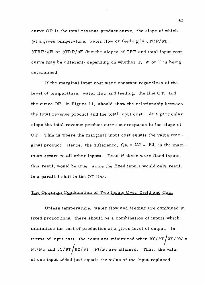
curve OP is the total revenue product curve, the slope of which
(at a given temperature, water flow or feeding)is 3TRP/9T,
9TRP/9W or 9TRP/9F (but the slopes of TRP and total input cost
curve may be different) depending on whether T, W or F is being
determined.
If the marginal input cost were constant regardless of the
level of temperature, water flow and feeding, the line OT, and
the curve OP, in Figure 11, should show the relationship between
the total revenue product and the total input cost. At a particular
slopes the total revenue product curve corresponds to the slope of
OT. This is where the marginal input cost equals the value mar-
ginal product. Hence, the difference, QR = QJ - RJ, is the maxi-
mum return to all other inputs. Even if these were fixed inputs,
this result would be true, since the fixed inputs would only result
in a parallel shift in the OT line.
The Optimum Combination of Two Inputs Over Yield and Gain
Unless temperature, water flow and feeding are combined in
fixed proportions, there should be a combination of inputs which
minimizes the cost of production at a given level of output. In
terms of input cost, the costs are minimized when 9Y/9T/9Y/9'W =
Pt/Pw and 9Y/9T I dY/ d £ = Pt/Pf are attained. Thus, the value
of one input added just equals the value of the input replaced.
44
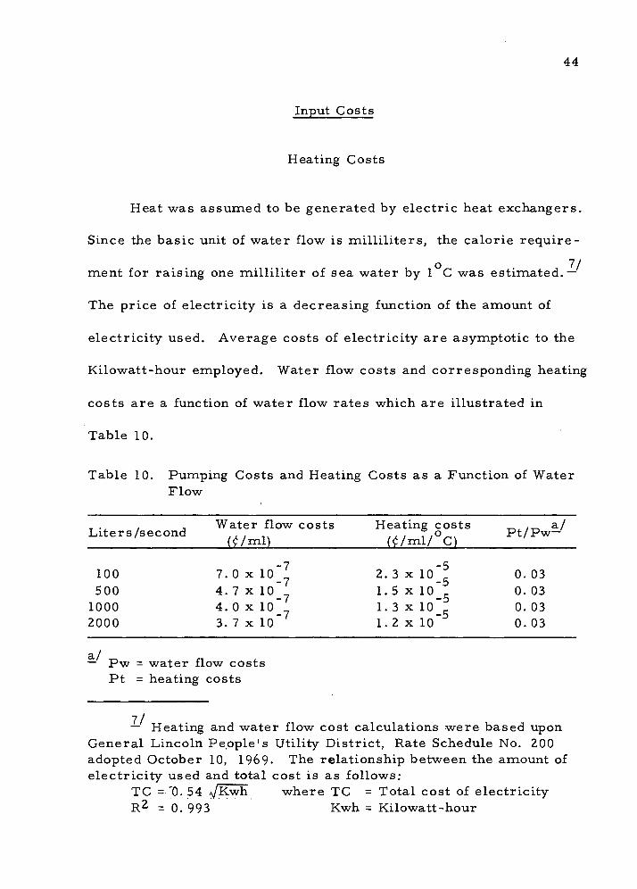
Input Costs
Heating Costs
Heat 'was assumed to be generated by electric heat exchangers.
Since the basic unit of water flow is milliliters, the calorie require-
ment for raising one milliliter of sea water by 1 C was estimated.—
The price of electricity is a decreasing function of the amount of
electricity used. Average costs of electricity are asymptotic to the
Kilowatt-hour employed. Water flow costs and corresponding heating
costs are a function of water flow rates which are illustrated in
Table 10.
Table 10. Pumping Costs and Heating Costs as a Function of Water Flow
_ ., , , Water flow costs Heating costs ^ ._ a/ Liters/second ,.. n> ,., f.o^ Pt/Pw— (I/ml) (l/ml/ C) [
100 7.0x10"^ 2.3x10";! 0.03 500 4.7x10" 1.5 xio" 0.03
1000 4.0x10" 1.3x10" 0.03 2000 3. 7 x 10 1. 2 x lo" 0. 03
a/ — Pw = 'water flow costs Pt = heating costs
— Heating and •water flow cost calculations were based upon General Lincoln People's Utility District, Rate Schedule No. 200 adopted October 10, 1969- The relationship between the amount of electricity used and total cost is as follows:
TC =-'0. 54 ijKwh where TC = Total cost of electricity R2 = 0. 993 Kwh = Kilowatt-hour
45
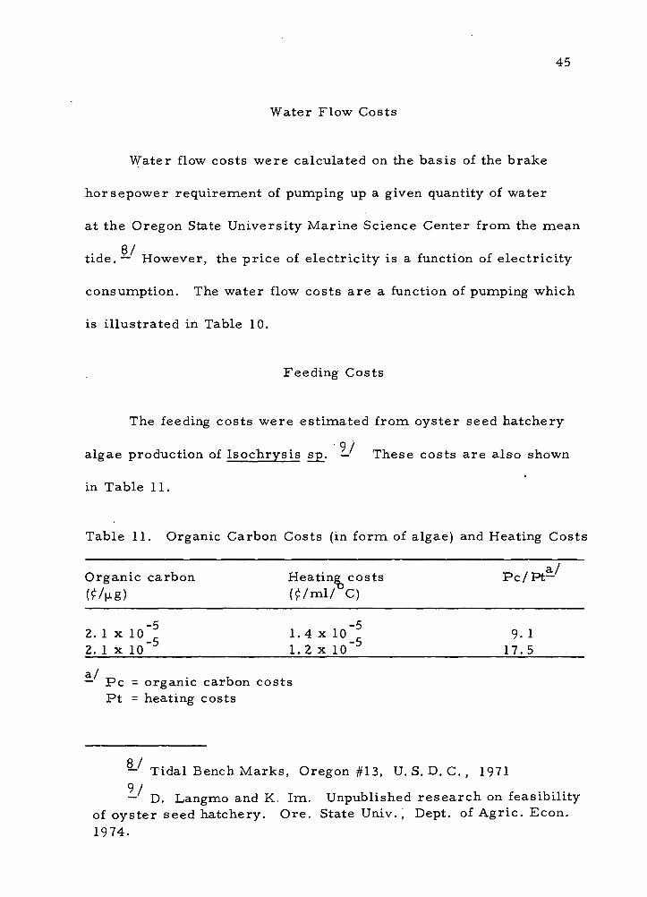
Water Flow Costs
Water flow costs were calculated on the basis of the brake
horsepower requirement of pumping up a given quantity of water
at the Oregon State University Marine Science Center from the mean
tide. — However, the price of electricity is a function of electricity
consumption. The water flow costs are a function of pumping ■which
is illustrated in Table 10.
Feeding Costs
The feeding costs were estimated from oyster seed hatchery
9/ algae production of Isochrysis sp. — These costs are also shown
in Table 11.
Table 11. Organic Carbon Costs (in form of algae) and Heating Costs
a/ Organic carbon Heating costs Pc/Pt— tfAig) tf/ml/ C)
2. 1 x 10"^ 1.4 x 10~5 9- 1 2. 1 x 10 1.2 x 10" 17.5
a/ - Pc = organic carbon costs Pt = heating costs
-' Tidal Bench Marks, Oregon #13, U. S. D. C. , 1971 9/ — D. Langmo and K. Im. Unpublished research on feasibility
of oyster seed hatchery. Ore. State Univ., Dept. of Agric. Econ. 1974.
46
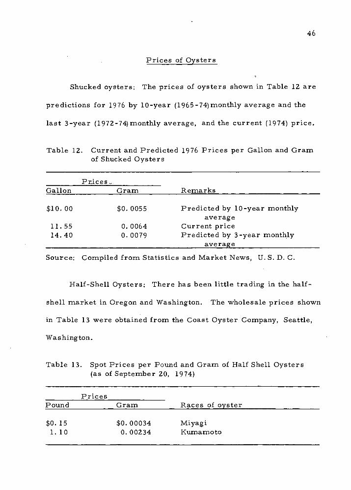
Prices of Oysters
Shucked oysters: The prices of oysters shown in Table 12 are
predictions for 1976 by 10-year (1965-74) monthly average and the
last 3-year (1972-74)monthly average, and the current (1974) price.
Table 12. Current and Predicted 1976 Prices per Gallon and Gram of Shucked Oysters
P rices „ Gallon Gram Remarks
$10. 00 $0.0055 Predicted by 10-year monthly average
11.55 0.0064 Current price 14.40 0.0079 Predicted by 3-year monthly
average
Source: Compiled from Statistics and Market News, U.S. D. C.
Half-Shell Oysters; There has been little trading in the half-
shell market in Oregon and Washington. The wholesale prices shown
in Table 13 were obtained from the Coast Oyster Company, Seattle,
Washington.
Table 13. Spot Prices per Pound and Gram of Half Shell Oysters (as of September 20, 1974)
Prices Pound Gram Races of oyster
$0.15 $0.00034 Miyagi 1.10 0.00234 Kumamoto
47
III. PRODUCTION FUNCTION ESTIMATES
The Nature of the Experiments
Newport Experiment III: Total Wet Meat Yield by Temperature and Water Flow
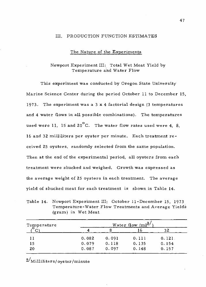
This experiment was conducted by Oregon State University
Marine Science Center during the period October 11 to December 15,
1973. The experiment was a 3 x 4 factorial design (3 temperatures
and 4 water flows in all possible combinations). The temperatures
used were 11, 15 and 20 C. The water flow rates used were 4, 8,
16 and 32 milliliters per oyster per minute. Each treatment re-
ceived 25 oysters, randomly selected from the same population.
Then at the end of the experimental period, all oysters from each
treatment were shucked and weighed. Growth was expressed as
the average weight of 25 oysters in each treatment. The average
yield of shucked meat for each treatment is shown in Table 14.
Table 14. Newport Experiment III: October 11-December 15, 1973 Temperature-Water Flow Treatments and Average Yields (gram) in Wet Meat
Tempe rature Water flow (ml*') (0c) 4 8 16 32
11 0.082 0. 091 0. Ill 0. 121 15 0. 079 0. 118 0. 135 0. 154 20 0. 087 0. 097 0. 148 0. 157
a/ — Milliliters/oyster/minute

48
Newport Experiment IV: Total Weight Gain by Temperature and Water Flow
This experiment was a 3 x 4 factorial design using the same
conditions and the same samples as in experiment III. Weight gains
were determined by measuring the shell length of all 25 oysters in
each treatment at the beginning and at the end of the experiment.
Weight gains were expressed as the difference between the initial
and final mean weights for each treatment. The total weight gains
for each treatment are shown in Table 14.
Table 15. Newport Experiment IV: October 11-December 15, 1973. Temperature-Water Flow Treatments and Average Gains (gram) in Total Weight a/
Temperature Water fl< DW (ml— ) f0C) 4 8 16 32
11 0. 021 0. 038 0.081 0. 132 15 0. 027 0. 086 0. 150 0.204 20 0.032 0.054 0. 102 0.290
a/ — Total weight is inclusive of shell h / —' Milliliters/oyster/minute
Newport Experiment V: Total Weight Gain by Temperature and Water Flow
This experiment was conducted in the same fashion as in
experiment IV, but the water flows used were 4, 16, 28 and 40
milliliters per oyster per minute. Weight gains were expressed as

49
the difference between the initial and final mean weights for each
treatment. The average total weight gains for each treatment are
shown in Table 16.
Table 16. Newport Experiment V; May 16-July.'.15, 1974. Temperature-Water Flow Treatments and Average Gain (gram) in Total Weight a/
Tempei rature Water flow (ml- ./)
(0c) 4 16 28 40
11 1.21 3.09 4. 16 4.31 -
15 1.31 3.53 4.50 5. 77 20 1.08 1.77 3. 72 6. 17
a/ — Difference in gain between experiment IV and V was due to a difference in food availability by season (i. e. , experiment IV was in winter, •whereas experiment V was in summer)
b/ — Milliliter$/oyster/minufce
Newport Experiment VI: Total Weight Gain by Temperature and Organic Carbon Supply
The experimental conditions were the same as experiment V,
but water flow was replaced as a variable by organic carbon count.
During the sixth experiment, the organic carbon content of a given
quantity of sea water was monitored for a 24-hour period once a week.
Since, during summer time, organic carbon supplies from non-
sea sources were negligible, —- the estimation of growth relation-
— Sources of organic carbon could be dissolved organic carbon, seaweeds, plankton (phyto and zoo) and so on.

50
ships between temperature and organic carbon was attempted,
assuming that oysters would take any organic matter in the sea
water and utilize it for growth. From the experiment conducted by
the School of Oceanography at Oregon State University, the amount
of organic carbon and the algae equivalency were estimated.—
Table 17. Newport Experiment VI: May 16-July 15, 1974. Temperature-Organic Carbon (Algae, Isochrysis sp. ) Treatments and Average Gains (grams) in Total Weight
Temper-/ |ag^ .. 5.56 22.24 38.92 55.60 , ature / # of algae- 3.9x10 1.6x10 2.7x10 3.9x10 o '
( C)
u. 15 20
a/ — Organic carbon (figj/pyster/minute u / — Number of algae/oyster/minute
1.21 3.09 4. 16 4.31 1.31 3.53 4.50 5.77 1.08 1. 77 3.72 6. 17
— The estimation of the level of algae requirement was inferred from the equation of monocultured algae, Isocrysis sp. , and the organic carbon content of the algae.
A = 70384C
R = 0.989
where A: number of algae C: organic carbon ((j,g)
Caution should be used in the interpretation of the level of algae equivalency, since the organic carbon content of algae may vary according to environmental factors and the growth stage of algae.

51
Production Function Specification
Since little previous study in aquaculture has been done in
deriving equations with one or two inputs, the primary consideration
in the selection of a production function is that the mathematical
characteristics or restrictions of the function must fit the biological
relationships involved. The requirements of the production function
are that (1) it must allow decreasing productivity to each unit of
input, since the higher the stage of growth the greater the amount
of energy needed to maintain an organism, (2) the capacity to in-
crease output by an increase in the application level of one input is
limited by the levels of other inputs, and (3) as oysters increase in
size the changes in body composition are expected to cause changes
in substitution rates between inputs. Heady et al. , (1955, p. 303)
listed five possible equations to explain the production relationships
between crops and fertilizer application.
(12) " • ' ~ ' "2
(13)
(14)
(15)
(16) Y = a + bF + cF2 + d ^/F"
The production function of the types (13) and (14) do not fulfill
all of the mathematical requirements stated above. A major
Y = a + bF + cF"
Y = m - ar F
Y = aFb
Y = a + bF + CsjF

52
disadvantage of the Cobb-Douglas type function is that if b (power)
is greater than zero, the equation will imply a continually increasing
yield with respect to that input. It would reach neither a maximum
nor a limiting output, if inputs were increased proportionally. Such
an implication is inconsistent with biological phenomena. That is,
even if all inputs are increased by the same proportion, high tem-
perature, for example, will kill oysters by heat exhaustion.
A simple parabolic function of the form, (12), where a minus
sign before C would denote a diminishing marginal rate of returns,
does not impose the restrictions common to the power function or
the exponential function. It allows both a declining and a negative
marginal productivity.
A variation of the quadratic form, used in most of the fertilizer
application studies (Heady et al. , 1955; Brown et al. ; 1956; Baum
et al. , 1956) took the form of (15). This form allows for a dimin-
ishing marginal rate of return. The equations (15) and (16) produce
a curve which turns down more slowly than the equation (12). The
function increases more rapidly at the beginning of the factor applica-
tion (if C<0)) which might somewhat better describe the biological
properties of organisms.

53
Regression Results
Tables 14, 15, 16 and 17 show that on the average, water flow
yields a greater growth response than temperature, and that the
interaction between temperatures and water flows results in higher
yields. The equations, which were statistically acceptable, were
used in deriving the "best fit" production function. The results of
the statistical analysis are shown in Tables 18, 20, 22 and 24.
A square root transformation of input interaction and a square
transformation of temperature were fitted to the 12 observations of
experiment III included in Table 14. The resulting curvilinear
equation is equation (17).
A square and square root transformation, of. the temperature
of the quadratic equation (18) was fitted to the data of experiment IV.
A square transformation of input interaction and fourth power trans-
formation of teraperature was fitted to the data of experiments V
and VI (eqs. 19 and 20). These specifications of the regression
equations gave the best fit because they explained more of the varia-
tions; each of the regression coefficients showed a significant con-
12/ tribution to the explanation of the dependent variable.-— The
12/ — Criterion used in selecting production functions were t value of each coefficient and R of each equation, in addition to the specification described in the preceding section.

54
transformed equations allow (1) diminishing marginal rates of
return (eq. 17 and 18), (2) diminishing marginal rates of substitu-
tion, and (3) changes in substitution rates at a ratio line (eq. 17,
18, 19 and 20).
These are as follows:
(17) Y = 0. 0046696T - 0.0033235W + 0. 010931\/TW-. 0.00024191T2
m
(18) Gt =-0.4917 - 0. 0022987W + 0. 1823 JT + 0. 00057373TW
-0. 00085433T2
(19) Gt = 0. 15245T + 0. 008941W + 0. 000004266T2W2
-0. 000015534T
(20) Gt = 0. 15245T + 0. 049598C + 0.0000022081T2C
-0. 000015534T4
where
Y = predicted growth in grams of meat (eq. 17)
Gt = predicted gain in grams of total weight (eqs. 18, 19 and 20)
o T = temperature level ( C)
W = water flow rate (milliliters/oyster/minute)
TW = interaction between temperature and water flow
C = organic carbon (jjig/oyster/minute) (eq. 20)
TC - interaction between temperature and organic carbon (eq. 20)

55
The t values of the regression coefficients are shown in
Tables 18, 20, 22 and 24. The t values indicate the statistical
significance of the contribution of the independent variables,
hypothesizing that the coefficients of each of the independent varia-
bles are not equal to zero against the null hypothesis that coeffi-
cients in the independent variable were equal to zero.
The constant terms were dropped from equations (17), (19)
and (20). The constant terms in those equations were found to be
not significant (at 30 percent significance level). By dropping the
constant, the equation would gain a degree of freedom, and
13/ thereifore improve the t values.— It is also reasonable
to assume that, if temperature and water flow were equal to zero,
oysters at best would gain no weight.
13/ — J. Neter and W. Wasserman (1974, p. 159) state that "When it is known that (3 =0, one could still use the general model (e.g., y = p + (3 x. + e.), anticipating that b will differ from zero only by a small sampling error. However, it is more efficient to incorporate the knowledge (3=0 into the model, thereby gaining a degree of freedom and simplifying the calcu- lations. ..." (However) "The model (e.g. y = (3 x. + e.) should be evaluated for aptness. Even though it is known that the regression function must go through the origin, the function might not be linear other than in the observed area. "
56
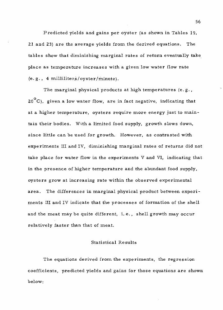
Predicted yields and gains per oyster (as shown in Tables 19,
21 and 23) are the average yields from the derived equations. The
tables show that diminishing marginal rates of return eventually take
place as temperature increases with a given low water flow rate
(e.g., 4 milliliters/oyster/minute).
The marginal physical products at high temperatures (e.g. ,
20 C), given a low water flow, are in fact negative, indicating that
at a higher temperature, oysters require more energy just to main-
tain their bodies. With a limited food supply, growth slows down,
since little can be used for growth. However, as contrasted with
experiments III and IV, diminishing marginal rates of returns did not
take place for water flow in the experiments V and VI, indicating that
in the presence of higher temperature and the abundant food supply,
oysters grow at increasing rate within the observed experimental
area. The differences in marginal physical product between experi-
ments III and IV indicate that the processes of formation of the shell
and the meat may be quite different, i. e. , shell growth may occur
relatively faster than that of meat.
Statistical Results
The equations derived from the experiments, the regression
coefficients, predicted yields and gains for those equations are shown
below:

57
Newport Experiment III: Total Wet Meat Yield (gram) by Temperature and Water Flow
(17) Y = 0. 0046696T - 0.0033235W+ 0. 010931\/TW~ 0. 00024191T m.
R2 = 0. 933
Table 18. Newport Experiment III: Regression Coefficients and t Values for the Total Wet Meat Yield (gram ) Function
Independent Regression t Significance variables coefficients Values levels ( %) a/_
2
.5
1
1 _
- Probability of obtaining as large or a larger value of t by chance, given the hypothesis that the variables do not affect yield.
Table 19. Newport Experiment III: Predicted Yield (gram) Per Oyster for Various Temperatures and Water Flows
T 0.46696 x lo" 3.3038
W -0.33235 x lo" -2.5771
TW 0.10931 x 10"1 4.2481
T2 0.24191 x 10"3 -4.9731
Temperature Water
a/ flow (ml- )
(0C) 4 8 16 24 32
11 0.08111 0.0978 0.1137 0.1197 0.1201 13 0,0851 0.1044 0. 1240 0., 1327 0. 1362 15 0.0869 0.1085 0.1315 0.1430 0.. 1485 17 0. 0860 0. 1100 0.1362 0.1513 0- 1577 20 0. 0807 0.1079 0. 1385 0.1560 0o 1664
a/ — Milliliters/oyster/minute
58
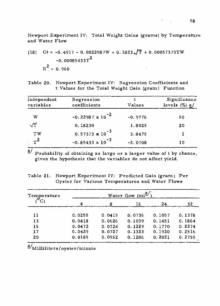
Newport Experiment IV: Total Weight Gains (grams) by Temperature and Water Flow
(18) Gt = -0. 4917 - 0. 0022987W + 0. 1823 JT + 0. 00057373TW
-0. 00085433T2
R2 = 0.960
Table 20. Newport Experiment IV: Regression Coefficients and t Values for the Total Weight Gain (gram) Function
Independent Regression t Significance variables coefficients Values levels (%) a/
W -0.22987:x 10"2 -0.9776 50
N/T 0. 18230 1.8025 20
TW 0,57373 x 10"3 3.8475 1
■ T2 -0.85433 x 10"3 -2.0708 10
a/ - Probability of obtaining as large or a larger value of t by chance,
given the hypothesis that the variables do not affect yield*
Table 21. Newport Experiment IV: Predicted Gain (gram) Per Oyster for Various Temperatures and Water Flows
Ternperature Water flow (ml-^
4 8 16 24 32
n 0.0255 0. 0415 0.0736 0.1057 0.1378 13 0.0418 0.0626 0.1039 0.1451 0.1864 15 0.0472 0-0724 0.1229 0.1770 0.2274 17 0.0429 0.0727 0.1323 0.1920 0.2516 20 0.0185 0.0552 0.1286 0.2021 0.2755
a/ — Milliliters/oyster/minute
59
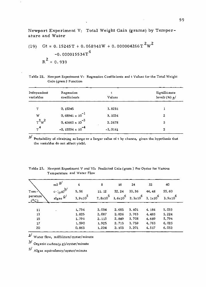
Newport Experiment V: Total Weight Gain (grams) by Temper- ature and Water
(19) Gt = 0. 15245T + 0. 068941W + 0. 000004266T 2W2
-0.000015534T
R2 = 0. 939
Table 22. Newport Experiment V: Regression Coefficients and t Values for the Total Weight Gain (gram)' Function
Independent Regression t Significance variables coefficients Values levels (%) a^/
T 0.15245 3.8231 1
W 0.68941 x 10" 3. 1034 2 2 2 -5
T W 0.42660 x 10 2.2678 5 4 -4
T -0. 15534 x 10 -3.0141 2
2/ Probability of obtaining as large or a larger value of t by chance, given the hypothesis that the variables do not affect yield.
Table 23. Newport Experiment V and VI: Predicted Gain (gram ) Per Oyster for Various Temperature and Water Flow
\ ml^ 4 8 16 24 32 40
TemX c-(|j.g)~ 5.56 11. 12 22.24 33.36 44.48 55.60
peratureV (0C) \
algae 3.9x10 7.8xl05 6 1.6x10
6 2.3x10
6 3. 1x10 3.9xl06
11 1.734 2,034 2.685 3.401 4.184 5.033 13 1.825 2.087 2.826 3.763 4.483 5.224 15 1.791 2.113 2.849 3.708 4.689 5.794 17 1.590 1.925 2.713 3.759 4.763 6.025 20 0.863 1.224 2. 103 3.201 4.517 6.052
a/ — Water flow, milliliters/oyster/minute b/ — Organic carbon(|Xg)/oyster/minute c/
Algae equivalency/oyster/minute

60
Newport Experiment VI: Total Weight Gain (grams) by- Temperature and Organic Carbon
(20) Gt = 0. 15245T + 0. 049598C + 0. 0000022081T2C2
- 0.000015534T4
2 R = 0.939
Table 24. Newport Experiment VI: Regression Coefficients and t Values for Total Weight Gain (gram) Function
Independent Regression t Significance variables coefficients Values levels (%) a/
T 0.15245 3.8231 1
C 0.49598 x 10' -1 3.1034 2
T2C2 0.22081 x 10' ■5
2.3678 5
T4 -0. 15534 x 10' -4 -3.0141 2
a/ — Probability of obtaining as large or larger value of t by chance, given the hypothesis that the variables do not affect yield.
Yield Isoquants
The isoquants were derived from the predicting equations,
(17., 18, 19 and 20). The isoquants show the various combinations
of the two pairs of inputs, temperature and water flow, or temper-
ature and organic carbon, that can be used to obtain a particular
yield.
The different slopes of the isoquants show the change in the
temperature required to maintain a given yield when a higher water

61
flo-w is applied and vice versa. That is, the slope of the isoquants
14/ indicates the rate of substitution between the two inputs.—
14/ — Input combinations have been expressed in terms of sub- stitution rates. In the biochemical processes of an organism one input may not substitute for another; however, a given output may be attained -with several combinations of inputs. This may be the case in oyster production, since temperature can never replace the nutrients that oysters need for growth. However, it may be true that at lower temperatures potential nutrients cannot be util- ized due to slow digestive process. Temperature and nutrients can be looked upon as substitutes for each other in attaining a given yield even though physiological substitution does not actually take place. The fact that similar yield increases can be attained with different combinations of inputs causes them to serve as substitutes in the decision-making process.
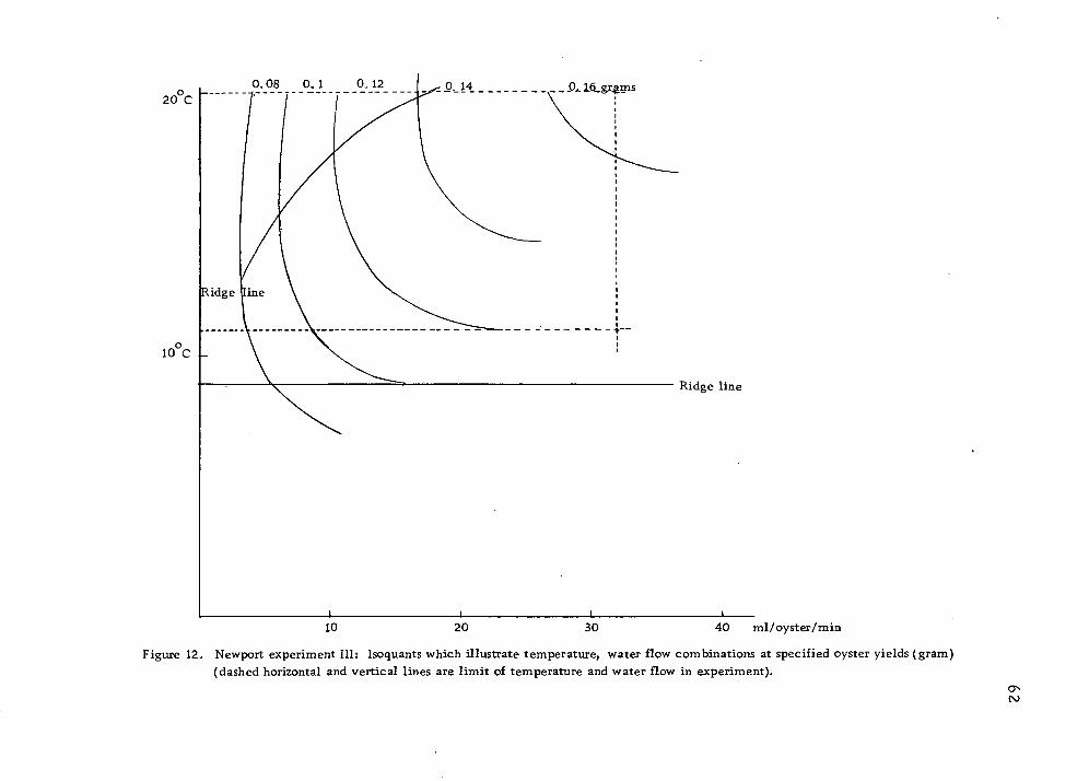
°- °A . . A1. . _ .O-.L2. — - ^-- 0=- it A. i6_&r^ms
„o 10 C
ml/oyster/min
Figure 12. Newport experiment III: Isoquants which illustrate temperature, water flow combinations at specified oyster yields (gram) (dashed horizontal and vertical lines are limit of temperature and water flow in experiment).

o 20 C
10OC
j ml/oyster/
Figure 13^ Newport experiment IV: Isoquants which illustrate temperature, water flow combinations at specified oyster gains (gram) (dashed horizontal and vertical lines are limit of temperature and water flow in experiment).

50 ml/oyster/min
Figure 14. Newport experiment V: isoquants which illustrate temperature, water flow combinations at specified oyster gains (gram ) (dashed
horizontal and vertical lines are limit of temperature and water flow in experiment) O *-

Expansion path (PC/PT=9. 1)
40 50 organic carbon (|jg)/pyster/min-
60
Figure 15. Newport experiment VI: Isoquants which illustrate temperature, organic carbon combinations at specified oyster gains (gram.) (dashed horizontal and vertical lines are limit of temperature and organic carbon supply in experiment).
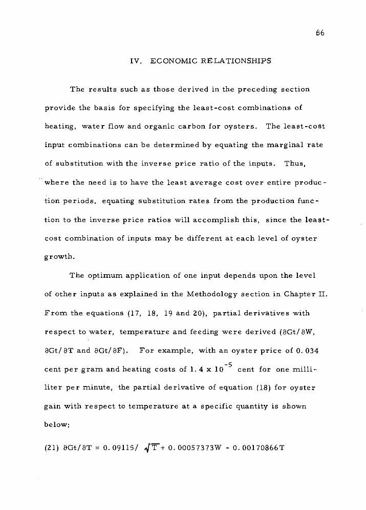
6-6
IV. ECONOMIC RELATIONSHIPS
The results such as those derived in the preceding section
provide the basis for specifying the least-cost combinations of
heating, water flow and organic carbon for oysters. The least-cost
input combinations can be determined by equating the marginal rate
of substitution with the inverse price ratio of the inputs. Thus,
where the need is to have the least average cost over entire produc-
tion periods, equating substitution rates from the production func-
tion to the inverse price ratios will accomplish this, since the least-
cost combination of inputs may be different at each level of oyster
growth.
The optimum application of one input depends upon the level
of other inputs as explained in the Methodology section in Chapter II.
From the equations (17, 18, 19 and 20), partial derivatives with
respect to water, temperature and feeding were derived (3Gt/3W,
dGt/dT and aGt/9F). For example, with an oyster price of 0. 034
-5 cent per gram and heating costs of 1.4 x 10 cent for. one milli-
liter per minute, the partial derivative of equation (18) for oyster
gain with respect to temperature at a specific quantity is shown
below:
(21) 9Gt/aT = 0. 09115/ Apr+ 0. 00057373W - 0. 00170866T
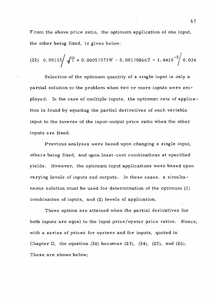
67
From the above price ratio, the optimum application of one input,
the other being fixed, is given below:
(22) 0. 09115/ ApT + 0. 00057373W - 0. 00170866T = 1.4xlo"5/ 0. 034
Selection of the optimum quantity of a single input is only a
partial solution to the problem when two or more inputs were em-
ployed. In the case of multiple inputs, the optimum rate of applica-
tion is found by equating the partial derivatives of each variable
input to the inverse of the input-output price ratio when the other
inputs are fixed.
Previous analyses were based upon changing a single input,
others being fixed, and upon least-cost combinations at specified
yields. However, the optimum input applications were based upon
varying levels of inputs and outputs. In these cases, a simulta-
neous solution must be used for determination of the optimum (1)
combination of inputs, and (2) levels of application.
These optima are attained when the partial derivatives for
both inputs are equal to the input price/oyster price ratios. Hence,
with a series of prices for oysters and for inputs, quoted in
Chapter II, the equation (20) becomes (23), (24), (25), and (26).
These are shown below;
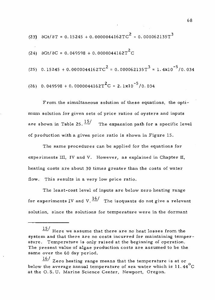
68
(23) 8Gt/8T = 0. 15245 + 0. 0000044162TC2 - 0. 000062135T3
(24) 9Gt/9C = 0. 049598 + 0. 0000044l62T2C
(25) 0. 15245 + 0. 0000044162TC2 = 0. 000062135T3 = 1. 4xlo"5/0. 034
(26) 0. 049598 + 0. 0000044162T2C = 2. lxlo"5/0. 034
From the simultaneous solution of these equations, the opti-
mum solution for given sets of price ratios of oysters and inputs
15/ are shown in Table 25.— The expansion path for a specific level
of production with a given price ratio is shown in Figure 15.
The same procedures can be applied for the equations for
experiments III, IV and V. However, as explained in Chapter 11,
heating costs are about 30 times greater than the costs of water
flow. This results in a very low price ratio.
The least-cost level of inputs are below zero heating range
for experiments IV and V. — The isoquants do not give a relevant
solution, since the solutions for temperature 'were in the dormant
15/ — Here we assume that there are no heat losses from the system and that there are no costs incurred for maintaining temper- ature. Temperature is only raised at the beginning of operation. The present value of algae production costs are assumed to be the same over the 60 day period.
— Zero heating range means that the temperature is at or below the average annual temperature of sea water which is 11.44 C at the O. S. U. Marine Science Center, Newport, Oregon.

Table 25. Optimum Temperature and Organic Carbon Application at Various Prices of Inputs and Output for Experiment VI
Given Resulting Oyster prices ((t/gram)
Imput costs Optimum input level ; Heating ; (j/mlA:)
Organic carbon
U/\!Z)
Temperature Organic carbon (|Jg/oyster/min)
Cains (grams)
Total revenue
_iD
Total feeding cost
m 0.034
0.243
1.4 x 10
1.2 x 10"
1.4 x 10
1. 2 x 10
3-5
-5 2. 1 x 10
2. 1 x 10
2. 1 x 10
2. 1 x 10
16.3
16.3
16.1
16.1
41.3
41.3
41.1
41. 1
4.48
4.48
4.41
4.41
0. 15
0.15
1.03
1.03
75.7
75.5
74.6
74.6

70
range and, biologically, in stage III for water flow, assuming that
the extrapolations outside of the observed experimental area are
accurate.
Tables 26 and 27 illustrate the maximum heating costs for
which it would be feasible to produce in stage II at various costs
of water flow. Marginal rates of substitution and price ratios for
heating and water flow can be found in experiment III. However,
the mathematical solution for experiment III was not only outside
of the observed experimental area but also the optimum temperature
is too high (i. e. , 28 C) for oyster production. (Oysters may
die from heat exhaustion. )
Two systems of feeding organic carbon to oysters may be
applied: (1) organic carbon (in the form of algae) is produced arti-
ficially and fed to the oysters by a recycled water system, or (2)
fresh sea water containing natural algae is heated and fed to the
oysters. The cost of producing organic carbon fed to the oysters
is about 2, 000 to 3, 000 times greater in method (1) compared to
method (2). However, the costs of heating the sea water under
method (2) are such that method (2) becomes 3-4 times more ex-
pensive than method (1). Solution for least-cost combinations of
organic carbon (in the form of algae) and temperature gives ex-
pansion path very close to upper ridge line. This is in spite of
the expansion path being congruent with lower ridge line when
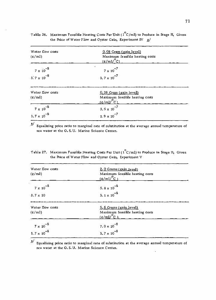
71
Table 26. Maximum Feasible Heating Costs Per Unit (1 C/ml) to Produce in Stage II, Given the Price of Water Flow and Oyster Gain, Experiment IV zj
Water flow costs 0, 08 Gram (gain level) (it/ml) Maximum feasible heating costs («t/ml/0C',
-8 " -7 7 x 10 7 x 10
-8 -7 3.7 x 10 3, 7x 10
Water flow costs 0. 26 Gram (gain level) (<t/ml) Maximum feasible heating costs ((t/ml/V)
-8 -7 7 x 10 3.5 x 10
-8 -7 3. 7 x 10 1.9 x 10
a/ Equalizing price ratio to marginal rate of substitution at the average annual temperature of sea water at the O. S. U. Marine Science Center.
o Table 27. Maximum Feasible Heating Costs Per Unit (1 C/ml) to Produce in Stage II, Given
the Price of Water Flow and Oyster Gain, Experiment V
Water flow costs 2, 0 Grams (gain level 1 ((t/ml) Maximum feasible heating costs
o (t/ml/ C \
-8 8 7 x 10 5. 8x 10"
-8 3.7 x 10 3. 1 x 10
Water flow costs 5. 6 Grams (gain level) Maximum (<t/ml/0C
(ct/ml) Maximum feasible heating costs ,o.
-8 -8 7 x 10 7. 0 x 10"
-8 -8 3, 7 x 10 3. 7 x 10
a/ — Equalizing price ratio to marginal rate of substitution at the average annual temperature of sea water at the O. S. U. Marine Science Center.
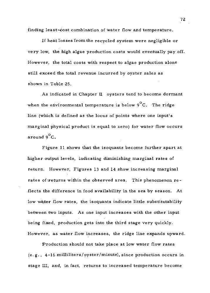
72
finding least-«ost combination of water flow aiid temperature.
If heat losses from the recycled system were negligible or
very low, the high algae production costs would eventually pay off.
However, the total costs with respect to algae production alone
still exceed the total revenue incurred by oyster sales as
shown in Table 25.
As indicated in Chapter II oysters tend to become dormant
when the environmental temperature is below 9 C. The ridge
line (which is defined as the locus of points where one input's
marginal physical product is equal to zero) for water flow occurs
around 9 C.
Figure 11 shows that the isoquants become further apart at
higher output levels, indicating diminishing marginal rates of
return. However, Figures 13 and 14 show increasing marginal
rates of^returns within the observed area. This phenomenon re-
flects the difference in food availability in the sea by season. At
low water flow rates, the isoquants indicate little substitutability
between two inputs. As one input increases with the other input
being fixed, production gets into the third stage very quickly.
However, as water flow increases, the ridge line expands upward.
Production should not take place at low water flow rates
(e.g. , 4-16 milliliters79ystef/minute), since production occurs in
stage III, and, in fact, returns to increased temperature become

73
negative.
If oysters were raised under controlled conditions, with a
reduction in the time required for maturity, the temperature level
would have to be higher than that of the natural environment. If
higher temperatures were used, higher water flow ■would have to
be implemented to be within the economic region (stage II).
Normally, the optimizing solution for economic analysis will
occur between the ridge lines. However, optimizing solution for
the economic analysis in this case occurs between the upper ridge
line and annual average sea water temperature (11.44 C) for
experiments III, IV and V. The annual average sea water temper-
ature can be considered as being equal to zero in economic scale.
The input is heat and at 11. 44 C no heat is being added.
Figure 16 (A and B) shows relevant biological relationship
and economic relationship. The ridge lines aa' and bb' were de-
rived from the production function. The bb' ridge line represents
dormancy as discussed in Chapter II. The area between the lines
cc' and zero axis in B of Figure 16 is the only relevant range for
economic analysis for this particular case. Below 11.44 C heat
must be removed (negative input). However, for the purpose of
illustration heat added is measured in terms of resulting tem-
o perature of water ( C).

11.44
Relevant biological relationship
(A)
Ridge line
Relevant economic relationship
(B) c'
Ridge line
Water flow (ml)/oyster/min
Ridge line
Water flow (mlj/oyster/min
d' Ridge line
Figure 16. Relevant biological relationship and economic relationship with average annual sea water temperature at 11.44 C
4^

75
Although the experiments were conducted in the same period
and conditions, there were differences in isoquants between ex-
periments III and IV. However, they could be explained as follows;
(1) the production function (18) is the gain function vis-a-vis the
production function (17) which is the yield function where equal
initial weight of oysters is assumed, and (2) the formation of shell
and meat may be a different process and shell formation may re-
quire less nutrients (mostly inorganic substances) than that of meat
(mostly organic substances).
76
V. SUMMARY AND CONCLUSIONS
Efforts in this study were directed towards:
(1) gaining insights into the recent trend of the oyster
industry in North America,
(2) identifying the problems of the industry that may be solved
by oyster production under controlled conditions,
(3) biological literature reviews to determine the critical
controllable variables for the production function estimates,
(4) the estimation of relationships among the identified vari-
ables and production from the experimental data,
(5) the estimation of costs associated with these controllable
variables, and
(6) the economic feasibility of oyster production under con-
trolled conditions with respect to these controllable variables..
The U. S. oyster industry has numerous problems, and its
production has been declining for 20 years. The major problems of
the industry identified in this study were as follows:
(A) the random fluctuations in natural seed supply on which
the industry is heavily dependent,
(B) natural disasters and predators, particularly on the East
Coast,
(C) pollution,

77
(D) oyster disease (e.g., MSX),
(E) limited changes in technology,
(F) stringent regulation regarding the use of common
property,
(G) an increasing demand for alternate use of common
property, and
(H) increasing competition from foreign countries.
Among identified problems, oyster production under con-
trolled conditions could overcome (A), (B), (C), (D) and (E),
and possibly (F) and (G).
The following variables were identified as biologicially
critical in order to achieve production under controlled environ-
mental conditions:
W = water flow (milliliters/oyster/minute)
F = feeding [organic carbon (jxg)/oyster/fninute]
T = temperature ( C)
0_ = dissolved oxygen (micromilliliters/oyster/minute)
P = pH
S = salinity (ppt)
A general oyster production function was of the form;
Y = f (W, T, F, 02, P, S, Xj, ..., Xn)
Y = yield Xi = unspecified factors affecting oyster growth
where

78
However, the relative significance of dissolved oxygen, pH and
salinity were found to be less critical in terms of costs. Thus, the
framework of oyster production could be expressed as follows;
Y = f (W, T, F | 02, P, S, X1, . . . , Xn)
But if food were supplied through sea water, the food supply would
be a function of water flow. Therefore, the production function
would be of the form for the once-through-sea water system;
Y = f[g(w)f T | 02, P, S, X1 XJ
Or, if food were supplied by artificial feeding and water were re-
cycled (assuming water and dissolved oxygen requirements are
minimum at a given temperature), then the equation would be of
the form;
Y = f (F, T|W, 02, P, S, X1, ..., Xn)
These models developed above were fitted to the data obtained
from the experiments conducted by the Department of Fisheries
and Wildlife, Oregon State University, at Newport, over a 2-y£ar
period from 1973 to 1974. The experiments were designed (1)
to investigate the effects on salmon and oyster production of the
application of effluent from a (possible) nuclear power plant in the
Pacific Northwest, (2) to investigate the seasonal changes in growth
patterns due to changes in natural food supply, and (3) to identify

79
what constitutes the biologically optimum water flow and temper-
ature without artificial feeding.
The four models, examined in Chapter III, estimated para-
meters involved in predicting the total yields and gains. The equa-
tions were of the form;
(1) Ym = 0. 0046696T + 0. 0033235W + 0. 01093^TW
-0. 00024191T R = 0.933
(2) Gt =- -0.4917 - 0.0022987W + 0. 1823\/T + 0. 00057373TW
-0. 00085433T2
R2 = 0.960
(3) Gt =■ 0. 15245T + 0. 068941W + 0. 000004266T2W2
-0. 000015534T4
R = 0.939
(4) Gt = 0. 15245T + 0. 049598C + 0. 000002208T2C2
-0.000015534T4
R2 = 0. 939
where
Ym = predicted growth in grams of meat
Gt = predicted gain in grams of total weight
o T = temperature ( C)
W = water flow (milliliters/oyster/minute)
TW = interaction between temperature and water flow
80
C = organic carbon (^g)/oyster/minute
TC = interaction between temperature and organic carbon
The coefficients of determination were significant for ex-
periments III, V and VI. Interaction between these inputs was also
important in increasing growth. However, the absence of either
input prevents the growth of oysters.
The gain responses in the summer are superior to the winter,
reflecting the difference in food availability in sea by season. With
the basic physiological relationships estimated for the experiments,
an economic analysis could be made.
The original hypothesis was designed to test whether oyster
production under controlled conditions is economically feasible.
The results of the analysis indicate that the costs of heating and
algae must be near zero to make production under controlled con-
ditions economically feasible, with current and forecasted (1976)
prices of oyster. This conclusion is based upon the production
function estimate of the observed experimental area. However,
there may exist economies of size beyond the experimental area,
particularly for experiments V and VI in which oysters grew at
an increasing rate. In order to take these facts into consideration,
the electricity charge was calculated, at least to hold 100 tons of
oysters (assuming each oyster weighs 30 grams and 40 ml/oyster/
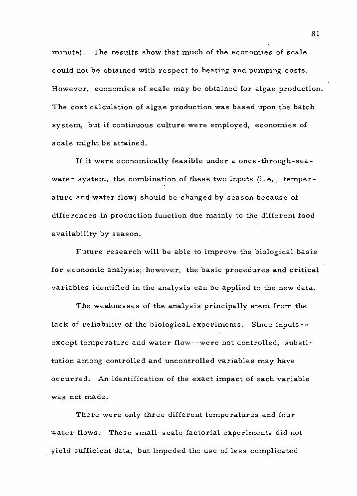
81
minute). The results show that much of the economies of scale
could not be obtained with respect to heating and pumping costs.
However, economies of scale may be obtained for algae production.
The cost calculation of algae production was based upon the batch
system, but if continuous culture were employed, economies of
scale might be attained.
If it were economically feasible under a once-through-sea-
water system, the combination of these two inputs (i.e., temper-
ature and water flow) should be changed by season because of
differences in production function due mainly to the different food
availability by season.
Future research will be able to improve the biological basis
for economic analysis; however, the basic procedures and critical
variables identified in the analysis can be applied to the new data.
The weaknesses of the analysis principally stem from the
lack of reliability of the biological experiments. Since inputs--
except temperature and water flow--were not controlled, substi-
tution among controlled and uncontrolled variables may have
occurred. An identification of the exact impact of each variable
was not made.
There were only three different temperatures and four
water flows. These small-scale factorial experiments did not
yield sufficient data, but impeded the use of less complicated

82
production functions (due mainly to multicollinearity problems).
Therefore, the use of polynominal estimating functions (fourth
power) for experiments V and VI may not reflect true relationships
between output gains and input levels, particularly outside of the
observed area.—
General recommendations for future studies concerned with
oyster culture under controlled conditions can be summarized as
follows:
(1) increase different levels of temperature and water flow
for factorial experiments. .This will increase the estimating
equations' precision, and, as a result, will minimize multicollin-
earity problems between transformations (e.g., T, T and l/T).
(2) concentrate biological observations in the relevant
economic region (stage 11) particularly at temperature levels above
15 C, water flow levels above 30 milliliters per oyster per minute
and organic carbon levels above 40 (jig per oyster per minute,
(3) control, or at least monitor, critical variables in
incoming and outgoing water,
— J. Neter and W. Wasserman (1974, p. 276) state that "Polynomial models with the independent variable present in high powers than the third are not often employed. The interpretation of the coefficients becomes difficult for such models, and they may be highly erratic for even small extrapolations. "
83
(4) control experiments by artificial feeding so that effects of
other unknown variables will be minimized in determining the effect
of feeding, and
(5) experiments should be conducted on the different stages
of growth, since the input requirements may change as oysters
reach a certain stage, and a different production function may be
required for different stages of growth (or if a once-through-sea-
water system were economically feasible, different combinations of
inputs should be employed by season as well), and--even if it is less
practical to often change feeding rates--as long as the revenues
incurred by changing feeding rates exceed the costs, that is the
least-cost method of production as well as giving a biologically
more accurate production function estimate.
84
BIBLIOGRAPHY
Amenia, I. Ecological Studies of Japanese Oyster, with Special Reference to the Salinity of their Habitats. J. Coll. Agr. Univ. Tokyo. 9: 333. 1928.
American Cyanamid Company. New Engineering Approaches for the Production of Connecticut Oysters: A Problem Analysis, Vol. 1 and 2. American Cyanamid Company, Connecticut. 1968. 308 p.
Bardach, J. E. and J. H. Ryther. The Status and Potential of Aquaculture. Amer. Inst. of Biol. Scie. 1968. 225 p.
Bardach, J. E. , J. H. Ryther and W. O. McLanncy. Aquaculture. New York, John,Wiley and Sons. 1972. 868 p.
Barrett, E. M. The California Oyster Industry. Res. Agen. of Calif., Dept. of Fish and Game. Fish Bull. 123: 1-103. 1963.
Baum, E. L. , E. O. Heady, J. T. Pesek and C. G. Hildreth. Economic and Technical Analysis of Fertilizer Innovations and Resource Use. Ames, Iowa. The Iowa State College. 1956. 398 p.
Baum, E. L. , E. O. Heady and J. Blackmore. Methodological Procedures in the Economic Analysis of Fertilizer Use Data. Ames, Iowa. The Iowa State College. 1956. 217 p.
Bell, F. W. The Factors Behind the Different Rates of.U.S. Fisheries. Div. of Econ. Res. Working Paper #13. 1969- 10 p.
Bilas, R. A. Microeconomic Theory, 2nd ed. New York, McGraw- Hill. 1971. 362 p.
Brown, W. G. , E. O. Heady, J. T. Pesek and J. A. Stritzil. Production Functions, Isoquants, Isoclines and Economic Optima in Corn Fertilization for Experiments with Two and Three Variable Nutrients. Ames, 1956. 25 p. (Iowa. Agri. Exp. Stat. Res. Bull. 441)
Butler, P. A. Reaction of Some Estuarine Mollusks to Environmental Factors. U. S. D. H. E. W. Working Paper #999. 25 p.

85
Burke, B. H. , B. Glenne and B. W. Adams. The Nearshore Physical Oceanographic Environment. Corvallis, 1971. Ref. 71-45. 127 p. (Oregon. Dept. Oceanog. , Oregon State University)
Chew, K. K. The Growth of a Population of Pacific Oysters (Crassostrea gigas) when Transplanted to Three Different Areas in the State of Washington. Doctoral Dissertation. Seattle, University of Washington, 1963. 192 p.
Claus, G. and C. Alder. Optimal Conditions for Oysters Grown in Closed Environments. Paper presented at Marine Technologi- cal Society Meeting. Washington, D. C. 1970. 8 p.
Current Fishery Statistics of the U.S. No. 6333. Dept. of Comm. 1973.
Davis, H. C. Survival and Growth of Larvae of the European Oyster, Ostrea edulis at Lowered Salinities. Biol. Bull. 122 (1): 33-9-
■1962.
Dean, D. The Experimental Feeding of Oysters. Doctoral Dissertation. New Brunswick, Rutgers University. 1957. 108 p.
Emadi, H. Effect of Heated Oceanwater on the Growth of Three Species Oysters; Pacific, C. gigas, European, O. edulis, and Native, O. lurida. 1972. 11 p.
Engle, J. B. The Mollscan Shellfish Industry-Current Status and Trend. Proc. of the Nat. Shellf. Assoc. 56: 13-21. 1966.
Feng, S. Y. Paper presented at the Shellfish Culture Conference, Selden, New York. 1968.
Ferguson, C. E. Microeconomic Theory. Illinois, Richard D. Irwin. 1972. 565 p.
Fishery Statistics of the U.S. , 1950-1972, U. S. D. C. 1950-72.
Furfari, S. A. Depuration Plant Design. U.S. D. H. E. W. Publ. Health Serv. 1966. 119 P-
Galtoff P. S. The American Oyster, Crossostrea virginica Gmelin. U.S. Fish. Wildl. Serv. Fish Bull. 64: 1-480. 1964.
86
Heaven, D. Aspects of Biodeposition by Oyster and other Invertebrate Filter Feeders. Limnol. Oceanogr. 11(4): 178-88. 1966.
Heady, E. O. , J. T. Pesek and W. G. Brown, Crop Response Surfaces and Economic Optima in Fertilizer Use. Ames, 1955. p. 292-332. (Iowa. Iowa State College. Agri. Exp. Stat. Res. Bull. 424)
Henderson, J. M. and R. E. Quandt. Microeconomic Theory. New York, McGraw-Hill. 1971. 431 p.
Imai, T. (ed. ) Kanzenyoshoku (in Japanese). Tokyo, Koseisha- Koseikaku. 1971. 454 p.
Imai, T. and S. Sakai. Study of Breeding of Japanese Oyster, Crassoshea gigas. Tohoku Univ. J. Agri. Res. 12: 125-71. 1961.
Johnston, W. E. and P. C. Allen. Technology Assessment and the Direction of Future Research; Use of Computerized Budgeting for Lobster Aquaculture. Contri. Paper for Annual Meeting of the American Agricultural Economic Asso. , College Station, Texas, August 1974.
Kmenta, J. Elements of Econometrics. New York, The Macmillan Co. 1971. 655 p.
Korringa, P. Recent Advances in Oyster Biology. Quart. Rev. Biol. 27:339-65. 1952.
Langmo, D. and K. Im. Unpublished Research on Economic Feasibility on Oyster Seed Hatchery. Corvallis, Dept. of Agri. Econ. 1974.
Loosanoff, V. L. and H. C. Davis. Spawning of Oysters at Low Temperatures. Science III: 521-2. 1950.
. Requirements for Maturation of Gonads of Northern Oysters. Biol. Bull. 103(1): 80-96. 1952.
Matthiessen, G. C. and R. C. Toner, Possible Methods of Improving the Shellfish Industry of Martha's Vineyard, Duke's County, Mass. Mass., 1966. 138 p. (The Marine Research Founda- tion ).
87
Matthiessen, G. C. A Review of Oyster Culture and the Oyster Industry in North America. Woods Hole, 1970. 52 p. (Woods Hole Oceanogr. Inst. Contri. No. 2528).
Medawar, P. B. Size and Age. In; Legros Clark and P. B. Medawar (eds. ) Essay in Growth and Form. London, Oxford Press. 1945. p. 157-187.
Menzel, R. W. Reports on Commercial-Scale Oyster Planting Experiments in Bayou Bas Bleu and Bay Ste. Elaine Oil Field. Texas A&M Res. Proj. 9- 1952. 146 p.
Mori, M. Studies on Oyster Mass Mortalities in Matsushima Bay. IV. Sexual Maturity and Changes on Physiological Activities and Glucose Contents. Tohoku J. Agri. Res. 25: 49-63. 1965.
Neter, J. and W. Wasserman. Applied Linear Statistical Models. Illinois, Richard D. Irwin. 1974. 800 p.
Oregon. University. Dept. of Fish, and Wildl. , . Corvallis, Oregon. Use of Heated Sea Water for Farming Oysters and Salmon. 1974. 40 p.
Pereyra, W. T. Growth of the Pacific Oyster (Cra.ssostrea gigas Thunberg) in Various Exposure Situations, with Considera- tions of the Experimental and Methodological Difficulties Encountered. Master's Thesis. Seattle, University of Washington. 1961. 87 p.
Quayle, D. B. The Seasonal Growth of the Pacific Oyster (Ostrea gigas) in Ladysmith Harbor. Ann. Rept. Br. Columbia. Dept. Fish. 1951. p. 85-90.
Pacific Oyster Culture in British Columbia. Fish. Res. Bd. Can. 169: 1-92. 1969.
Seno, H. , J. Hori and D. Kusabe. Effects of Temperature and Salinity on the Development of the Eggs of the Common Japanese Oyster, Ostrea gigas Thunberg. J. Fish. Inst. Tokyo. 22: 1-41. 1965.
Sokoloski, A. A. The Role of Imports in the U. S. Oyster Market. College Park, 1970. 4 p. (University of Maryland, Extension Service)

88
Sparks, A. K. , and K. K. Chew. Preliminary Report on Growth and Survival of the Pacific Oyster in Washington Waters. Proc. Nat. Shellf. Assoc. 50: 125-32. 1961.
Tarr, M. A., M. I. Carr and R. E. Westly. Final Report of Investigations for the Lummi Aquaculture Project. Dept. Fish., Res. Div. , Washington State, p. 46. 1971.
Tenore, K. R. , J. C. Goldman and J. P Clarner. The Food Chain Dynamics of the Oyster, Clam, and Mussel in an Aquaculture Food Chain. J. Exp. Biol. Ecol. 12: 157-65. 1973.
Wallace, D. H. Industry's Appraisal of the Future of the Oyster Industry. Proc. of the Gulf Carib. Fish. Inst. Miami, p. 135-38. 1961.
Warren, C. E. and G. E. Davis. Laboratory Studies on the Feeding, Bioenergetics, and Growth of Fish. In; S. D. Gerking (ed. ) Biological Basis of Freshwater Fish Production. Oxford, Blackwell Scientific Publ. 1967. p. 175-214.
Windham, D. M. Economic Aspects of the Oyster. Proc. of the Oyster Culture Workshop. Sapelo Island, 1968. p. 41-9. (Georgia. Mar. Fish. Div. Georgia Contri. Ser. Numb. 6)
Woelke, C. E. Introduction of the Kumamoto Oyster, Ostrea (Cressostrea) gigas, to the Pacific Coast. Washington State Dept. Fish., Fish. Res. Paper. 1(3): 41-50. 1955.
Wolfe, J. W. Professor, Oregon State University, Dept. of Agri.. Engr. , Personal Communication. Corvallis, Oregon. August 15, 1974.

89
APPENDIX I
COST CALCULATIONS
Heating Costs
Heating cost calculations were based upon General Lincoln
People's Utility District, Rate Schedule No. 200. The basic unit of
water flow is milliliters per oyster per minute, and caloric require-
ment for raising one milliliter sea water by one degree centigrade
was calculated.— The calorie was converted into a common unit,
Kwh (Kilowatt-hour) which is the basis of electricity charge. The
conversion equations were as follows;
(1) Kwh = 859, 184 calories
(2) 859, 184 x T^TT x efficiencies = milliliters of sea water that can be raised by one degree centigrade by 1 Kwh
where 1. 00 = the specific gravity of pure water.
1. 05 = the specific gravity of sea water
efficiency = heat exchanger efficiency, expressed as decimal, 0. 9 (Johnston and Allen, 1974, p. 25).
— One calorie is the amount of heat required to raise the temperature of one gram of water by one degree. The specific gravity of sea water is about 1. 05, therefore sea water requires more energy than fresh water to increase its temperature by 1 C.
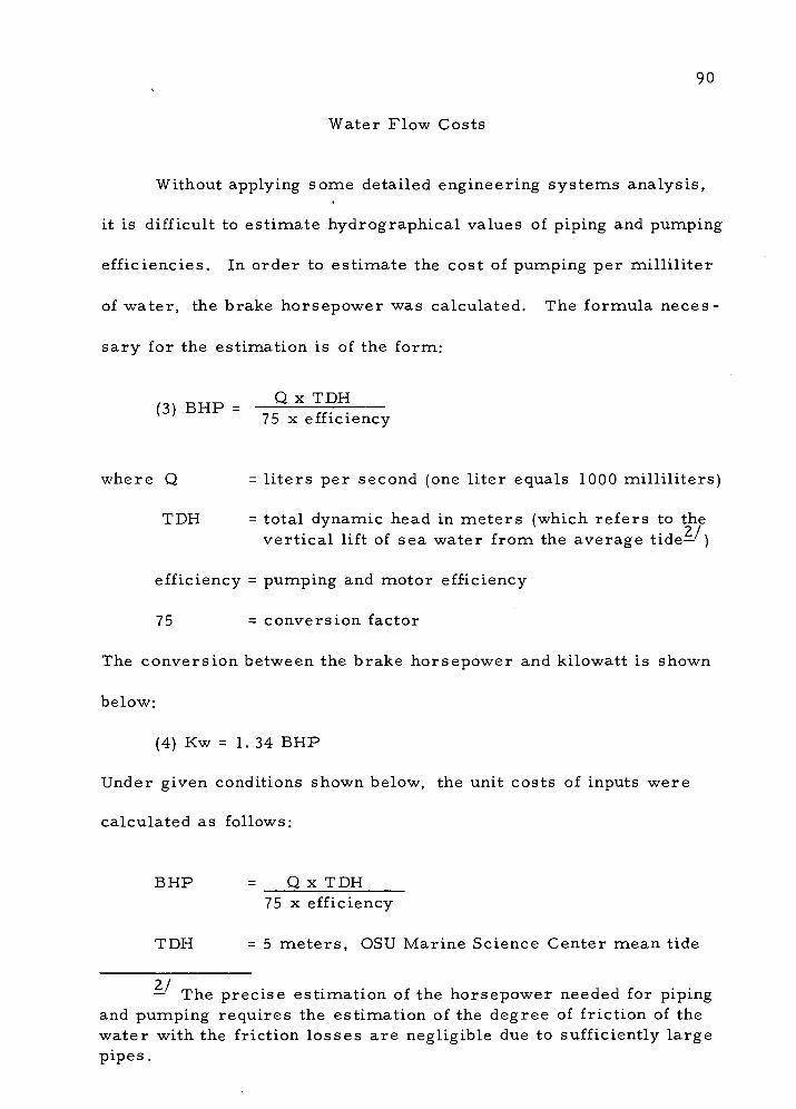
90
Water Flow Costs
Without applying some detailed engineering systems analysis,
it is difficult to estimate hydrographical values of piping and pumping
efficiencies. In order to estimate the cost of pumping per milliliter
of water, the brake horsepower was calculated. The formula neces-
sary for the estimation is of the form;
(3) BHP Q X TDH
75 x efficiency
where Q = liters per second (one liter equals 1000 milliliters)
TDH = total dynamic head in meters (which refers to the vertical lift of sea water from the average tide— )
efficiency = pumping and motor efficiency
75 = conversion factor
The conversion between the brake horsepower and kilowatt is shown
below:
(4) Kw = 1. 34 BHP
Under given conditions shown below, the unit costs of inputs were
calculated as follows;
BHP = Q x TDH 75 x efficiency
TDH = 5 meters, OSU Marine Science Center mean tide
2/ — The precise estimation of the horsepower needed for piping and pumping requires the estimation of the degree of friction of the water with the friction losses are negligible due to sufficiently large pipes.
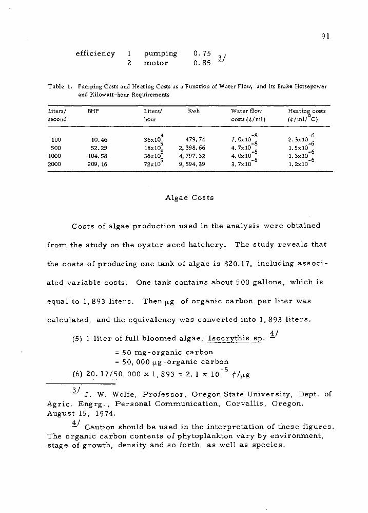
91
efficiency 1 pumping 0.75 . 2 motor 0. 85 -
100 10.46 36x10
18x10
36x10
72x10
479.74
500 52.29 2,398.66
1000 104.58 4, 797. 32
2000 209.16 9, 594. 39
Table 1. Pumping Costs and Heating Costs as a Function of Water Flow, and its Brake Horsepower and Kilowatt-hour Requirements
Liters/ BHP Liters/ Kwh Water flow Heating costs second hour costs ((t/ml) (it/ml/ C)
-8 -6 7.0x10 „ 2.3x10
-8 -6 4.7x10 1.5x10 4.0xl0~ 1.3x10"
-8 -6 3.7x10 1.2x10
Algae Costs
Costs of algae production used in the analysis were obtained
from the study on the oyster seed hatchery. The study reveals that
the costs of producing one tank of algae is $20.17, including associ-
ated variable costs. One tank contains about 5 00 gallons, which is
equal to 1, 893 liters. Then ^g of organic carbon per liter was
calculated, and the equivalency was converted into 1,893 liters.
4/ (5) 1 liter of full bloomed algae, Isocrythis sp. —
= 50 mg-organic carbon = 50, 000 (jig-organic carbon
(6) 20. 17/50, 000 x 1, 893 = 2. 1 x lo"5 tf/jig
3/ — J. W. Wolfe, Professor, Oregon State University, Dept. of Agric. Engrg. , Personal Communication, Corvallis, Oregon. August 15, 1974.
4/ — Caution should be used in the interpretation of these figures. The organic carbon contents of phytoplankton vary by environment, stage of growth, density and so forth, as well as species.
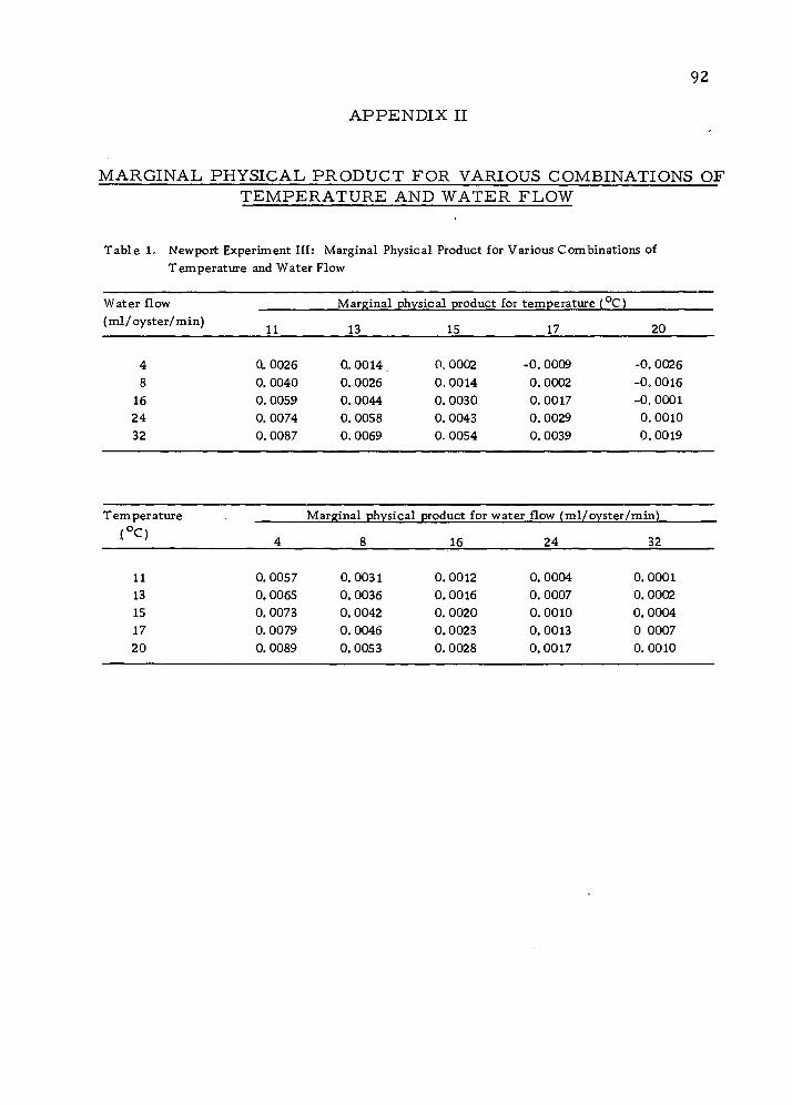
92
APPENDIX II
MARGINAL PHYSICAL PRODUCT FOR VARIOUS COMBINATIONS OF TEMPERATURE AND WATER FLOW
Table 1. Newport Experiment III: Marginal Physical Product for Various Combinations of Temperature and Water Flow
Water flow Marginal physical product for temperature (0C) (ml/oyster/min)
11 13 15 17 20
4 Q. 0026 Q.0014 0.0002 -0. 0009 -0. 0026 8 0. 0040 0. 0026 0.0014 0. 0002 -0. 0016
16 0. 0059 0.0044 0. 0030 0. 0017 -0. 0001 24 0. 0074 0. 0058 0. 0043 0. 0029 0.0010 32 0. 0087 0. 0069 0, 0054 0. 0039 0. 0019
Temperature Marginal physical product for water flow (m 1/oyster/min)
(0C) 4 8 16 24 32
11 0. 0057 0.0031 0. 0012 0.0004 0. 0001 13 0, 0065 0. 0036 0.0016 0. 0007 0.0002 15 0. 0073 0.0042 0. 0020 0. 0010 0. 0004 17 0. 0079 0. 0046 0. 0023 0. 0013 0 0007 20 0. 0089 0.0053 0. 0028 0.0017 0. 0010
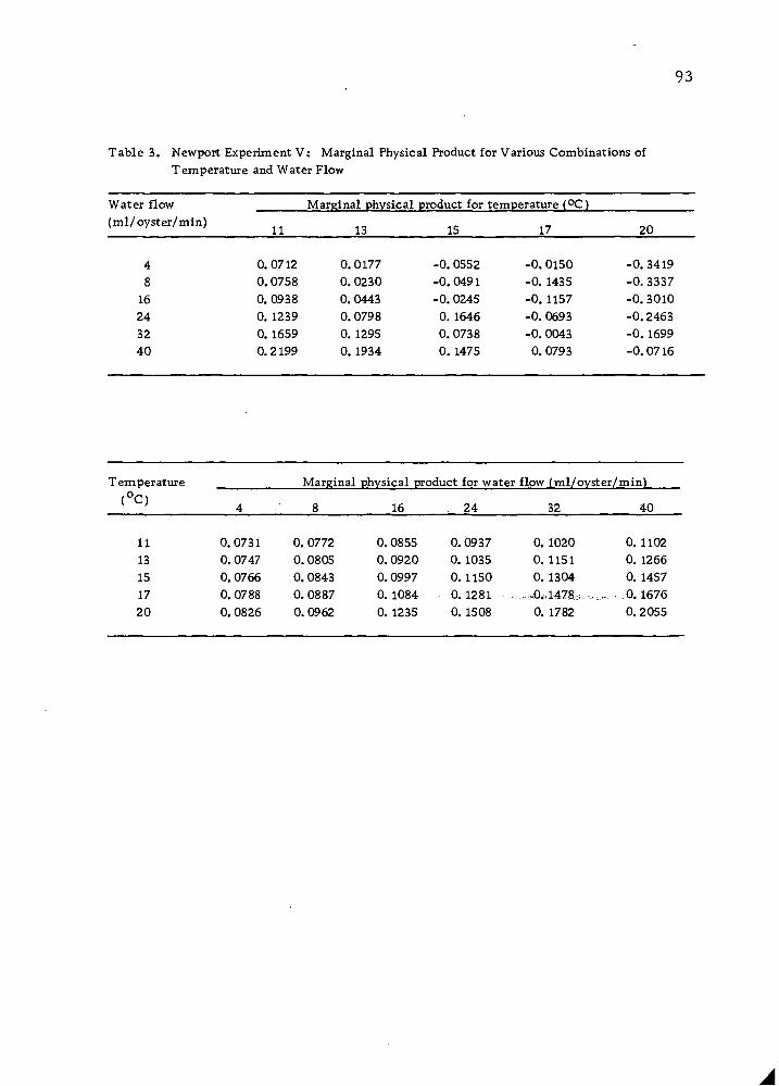
93
Table 3. Newport Experiment V; Marginal Physical Product for Various Combinations of Temperature and Water Flow
Water flow Marginal physical product for tem iperature (0C) (ml/oyster/min)
11 13 15 17 20
4 0.0712 0.0177 -0. 0552 -0. 0150 -0. 3419 8 0. 0758 0. 0230 -0.0491 -0. 1435 -0. 3337
16 0. 0938 0.0443 -0. 0245 -0. 1157 -0. 3010 24 0. 1239 0. 0798 0. 1646 -0. 0693 -0.2463 32 0. 1659 0. 1295 0. 0738 -0. 0043 -0.1699 40 0.2199 0. 1934 0. 1475 0. 0793 -0.0716
Temperature Marginal physical product for water flow (ml/oyster/min)
(0C) 4 8 16 24 32 40
11 0.0731 0. 0772 0. 0855 0. 0937 0. 1020 0. 1102 13 0. 0747 0. 0805 0. 0920 0. 1035 0. 1151 0. 1266 15 0. 0766 0. 0843 0. 0997 0. 1150 0. 1304 0. 1457 17 0. 0788 0. 0887 0. 1084 0. 1281 . ,...:«0.-vl47S.:i.-....,. 0.1676 20 0. 0826 0.0962 0. 1235 0. 1508 0. 1782 0. 2055

94
Table 2. Newport Experiment IV: Marginal Physical Product for Various Combinations of Temperature and Water Flow
Water flow Marginal physic :al product for temperature (0C) (ml/oyster/min)
11 13 IS 17 20
4 0.0110 0.0054 0. 0002 -0. 0046 -0,0115 8 0. 0132 0. 0077 0. 0025 -0. 0024 -0.0092
16 0, 0179 0.0122 0,0071 0.0022 -0. 0046 24 0„ 0225 0,0168 0.0117 0. 0068 -0. 00002 32 0. 0270 0.0214 0. 0163 0.0114 0.0046
Temperature Marginal physical product for water flows (ml/oyster/min)
(0C) 4 8 16 24 32
11 0. 0040 0. 0040 0.0040 0.0040 0. 0040 13 0. 0046 0.0046 0.0046 0.0046 0. 0046 15 0. 0063 0. 0063 0.0063 0. 0063 0. 0063 17 0. 0075 0. 0075 0. 0075 0. 0075 0. 0075 20 0. 0092 0. 0092 0.0092 0.0092 0. 0092
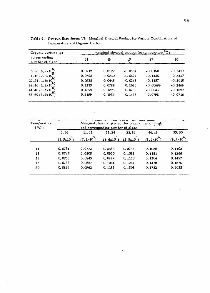
Table 4. Newport Experiment VI: Marginal Physical Product for Various Combinations of Temperature and Organic Carbon
95
Organic carbon (itg) corresponding number of algae
Marginal physical product for temperaturef C )
11 13 15 17 20
5.56 (3,9x10 ) 11. 12(7. 8x10 ) 22.24(1.6x10 ) 33. 36(2. 3x10 ) 44.48(3. 1x10 ) 55.60(3.9x10 )
0. 0712 0.0177 -0. 0552 -0.0150 -0. 3419 0. 0758 0. 0230 -0.0491 -0. 1435 -0. 3337 0. 0938 0. 0443 -0, 0245 -0.1157 -0. 3010 0. 1239 0. 0798 0.1646 -0. 00693 -0. 2463 0. 1659 0. 1295 0. 0738 -0. 0043 -0. 1699 0. 2199 0. 1934 0. 1475 0. 0793 -0.0716
Temperature Marginal physical product for organic carbon ((JLg^ (0C) and corresponding number of algae
5.56 11.12 22.24 33.36 44.48 55.60
(3;9xi05) (7.8xl05) (1.6x10 ) (2.3xl06) (3.IxlO6) (3.9xl06)
11 0.0731 0. 0772 0. 0855 0.0937 0. 1020 0.1102 13 0. 0747 0. 0805 0.0920 0, 1035 0. 1151 0. 1266 15 0„ 0766 0„ 0843 0.0997 0,1150 0. 1304 0. 1457 17 0. 0788 0. 0887 0.1084 0. 1281 0. 1478 0. 1676 20 0. 0826 0. 0962 0.1235 0.1508 0. 1782 0. 2055
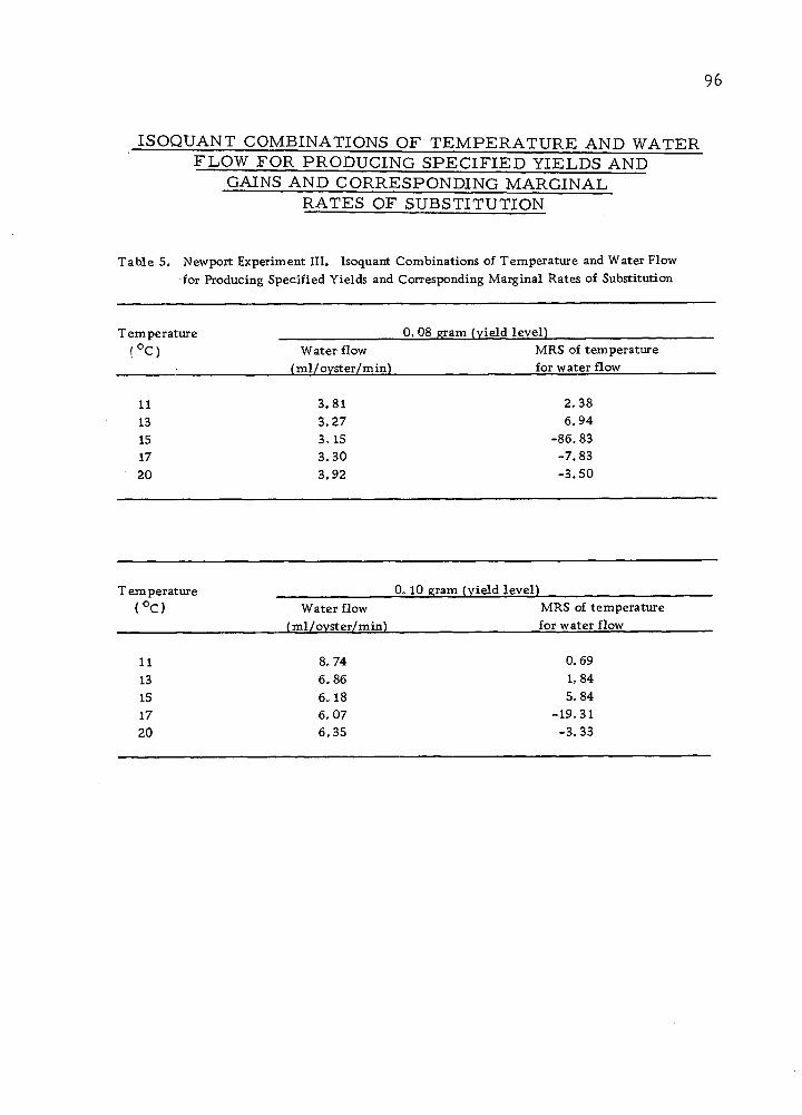
96
ISOQUANT COMBINATIONS OF TEMPERATURE AND WATER FLOW FOR PRODUCING SPECIFIED YIELDS AND
GAINS AND CORRESPONDING MARGINAL RATES OF SUBSTITUTION
Table 5. Newport Experiment III. Isoquant Combinations of Temperature and Water Flow for Producing Specified Yields and Corresponding Marginal Rates of Substitution
Temperature !0C) Water flow
(ml/oyster/min)
0, 08 gram (yield level) MRS of temperature for water flow
11 13 15 17 20
3.81 3.27 3.15 3.30 3.92
2.38 6.94
-86.83 -7.83 -3.50
Temperature (0C)
0,10 gram (yield level) Water flow
(ml/ovster/min) MRS of temperature for water flow
11 13 15 17 20
8., 74 6.86 6.18 6.07 6.35
0.69 1,84 5.84
■ 19.31 -3.33

97
Table 5. Newport Experiment III. Isoquant Combinations of Temperature and Water Flow for Producing Specified Yields and Corresponding Marginal Rates of Substitution --Continued
0, 12 gram (yield level) Temperature
(0C) Water flow (ml/oyster/min)
11 24.81 13 13.75 15 11.28 17 10.42 20 10.56
MRS of temperature for water flow
0.05 0.52 1.44 5.29
-4.08
Temperature (0c):-
0. 14 gram (yield level) Water flow
(ml/oyster/min) MRS of temperature for
water flow
11 13 15 17 20
No solution (imaginary number) No solution (imaginary number) 21.37 0.34 17. 74 1. 05 16.51 -48.77
Temperature (0C) Water flow
(ml/oyster/min)
0. 16 gram (yield level) MRS of temperature for
water flow
11 13 15 17 20
No solution (imaginary number) No solution (imaginary number) No solution (imaginary number) 36.23 0. 26.64 1.
16 17
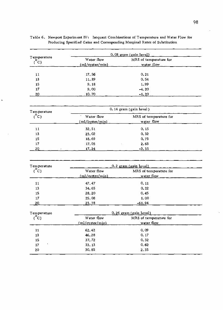
98
Table 6. Newport Experiment IV: Isoquant Combinations of Temperature and Water Flow for Producing Specified Gains and Corresponding Marginal Rates of Substitution
Temperature
(0c)
0. 08 gram (gain level) Water flow MRS of temperature for
(ml/oyster/min) water flow
17.56 0.21 11.39 0.54 9.18 1.99 9.00 -4.20
. 10. 70 -1.20
11 13 15 17 20
Temperature
(0c)
0. 14 gram (gain level)
Water flow (ml/byster/min)
MRS of temperature for water flow
11 13 15 17 20
32.51 23.02 18.69 17.03 17.24
0. 15 0.32 0.73 2.63
-2.35
Temperature
<0c) 0. 2 gram (gain level)
Water flow (ml/oyster/min)
MRS of temperature for water flow
11
13
15
17 20
47.47
34.65 28.20
25.08 23,78
0. 11 0.22 0.45 1.00
-61.94
Temperature
(0c) 0.26 gram (gain level)
Water flow (ml/oyster/min)
MRS of temperature for water flow
11 13
15 17
20
62.42 46.28
37.72
33. 13 30.85
0.09
0. 17
0.32 0.62 2.35

99
Table 7. Newport Experiment V: Isoquant Combinations of Temperature and Water Flow for Producing Specified Gains and Corresponding Marginal Rates of Substitution
Temperature
(0c) 2. 0 grains (gain level)
Water flow (ml/oyster/min)
MRS of temperature for water flow
11 13 15 17 20
7.56 6.29 6.63 8.84
15.15
0.99 3.61
-1.44 -0.57 -0.35
Temperature o
( C) 2>8 grams (gain levell
Water flow (ml/oyster/min)
MRS of temperature for water flow
11 13 15 17 20
17.34 15.72 15.50 16.80 21.27
0.99 2.22
-3.76 -0.98 -0.55
Temperature o
( C) Water flow (ml/oyster/min)
3.6 grams (gain level) MRS of temperature for water flow
11
13
15
17 20
26,09
23.92 23.06
23.53
26.57
0.99
1.67 12.69
-2.06
-0,84

100
Table 7. Newport Experiment V: Isoquant Combinations of Temperature and Water Flow for Producing Specified Gains and Corresponding Marginal Rates of Substitution— Continued
Temperature
(0c) 4. 4 gram^ (gain level)
Water flow (ml/oyster/min)
MRS of temperature for water flow
11
13
15
17 20
34.09
31.28
29.74
29.49
31.34
1.00 1.43 3.26
-7.31 -0.20
Temperature
(0c) 5. 2 grams (gain level)
Water flow (ml/oyster/min)
MRS of temperature for water flow
11 13 15
17 20
41.50
38.01
35.81 34.89
35.70
1.00 1.30 2.18
10.34 -2.25
Tern per ature
(0c)
6. 0 grams (gain level)
Water flow (ml/oyster/min)
MRS of temperature for water flow
11 13
15
17 20
48.44
44.25
41.40
39.85
39.75
1.00
1.23
1.78
3,86 -4.51
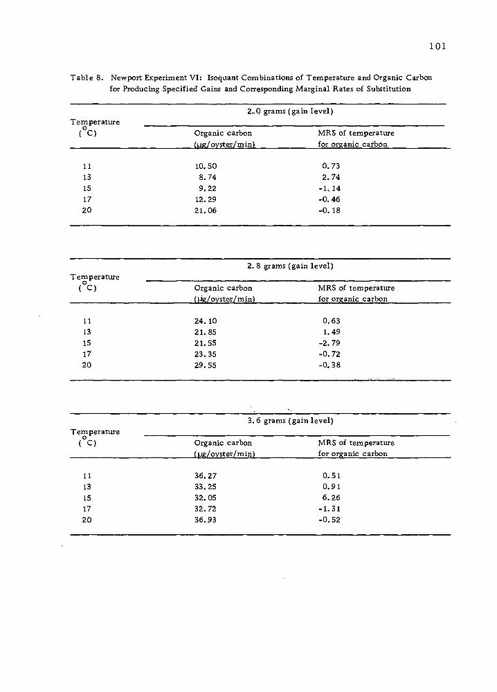
101
Table 8. Newport Experiment VI: Isoquant Combinations of Temperature and Organic Carbon for Producing Specified Gains and Corresponding Marginal Rates of Substitution
Tern per attire
(0c)
2„P grams (gain level)
Organic carbon
(^/oyster/min). MRS of temperature for organic carbon
11 13 15 17 20
10.50 8.74 9.22
12.29 21.06
0.73 2.74
-1,14 -0.46 -0.18
Temperature (0c)
2. 8 grams (gain level)
Organic carbon (Mg/oyster/min)
MRS of temperature for organic carbon
11 13 15 17 20
24. 10 21.85 21.55 23.35 29.55
0.63 1.49
-2.79 -0.72 -0.38
Temperature o
( C)
3, 6 grams (gain level)
Organic carbon (|jg/ovster/min)
MRS of temperature for organic carbon
11
13
15 17
20
36.27 33.25
32.05
32.72
36.93
0.51 0.91
6.26 -1.31
-0.52
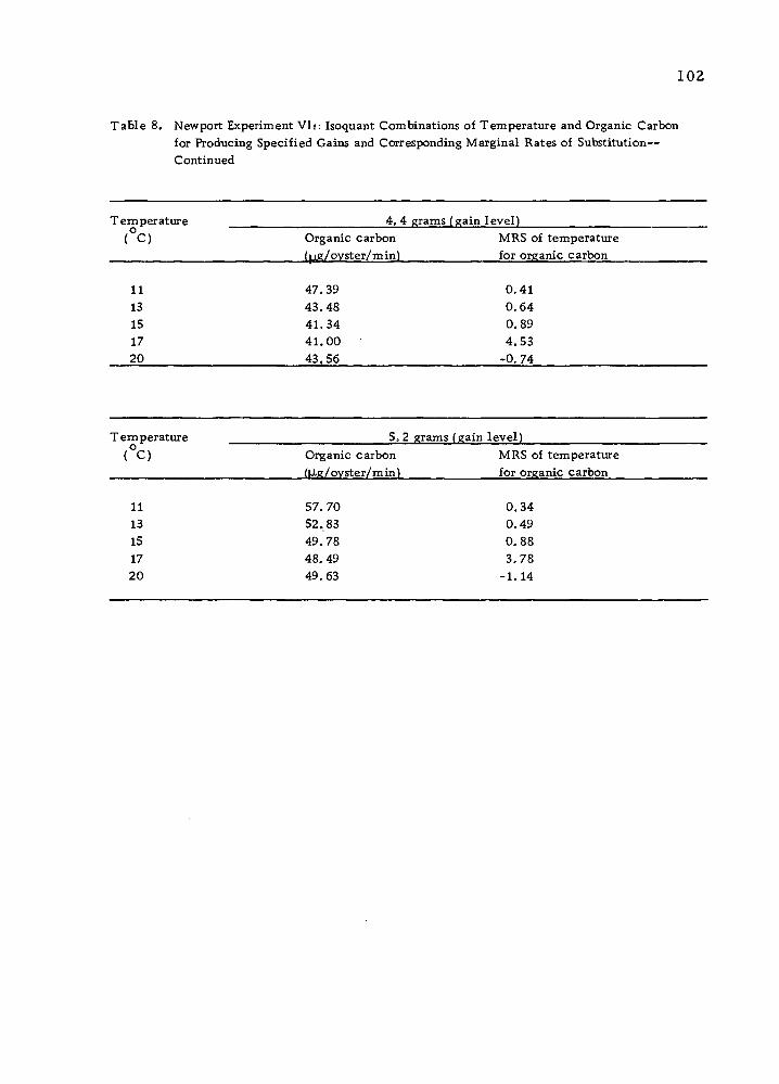
102
Table 8. Newport Experiment VIi: Isoquant Combinations of Temperature and Organic Carbon for Producing Specified Gains and Corresponding Marginal Rates of Substitution— Continued
Temperature (0c)
4. 4 grams (gain level) Organic carbon (ug/oyster/min)
MRS of temperature for organic carbon
11 13
15 17
20
47.39
43.48 41.34 41.00
43.56
0.41 0.64 0.89 4.53
-0.74
Temperature
(0c) 5. 2 grams (gain level)
Organic carbon (Ug/oyster/min)
MRS of temperature for organic carbon
11 13
15
17 20
57.70
52.83
49.78 48.49
49.63
0,34
0.49
0.88
3.78
-1.14


![FISICA GENERAL [Schaum Frederick J. Bueche]](https://img.dokumen.tips/doc/110x75/5492d79db479592e5a8b4792/fisica-general-schaum-frederick-j-bueche.jpg)


