Embed Size (px)
Citation preview

This is an Open Access document downloaded from ORCA, Cardiff University's institutional
repository: http://orca.cf.ac.uk/93616/
This is the author’s version of a work that was submitted to / accepted for publication.
Citation for final published version:
Marzano, Frank, Picciotti, Errico, Di Fabio, Saverio, Montopoli, Mario, Mereu, Luigi, Degruyter,
Wim, Bonadonna, Costanza and Ripepe, Maurizio 2016. Near-real-time detection of tephra eruption
onset and mass flow rate using microwave weather radar and infrasonic arrays. IEEE Transactions
on Geoscience and Remote Sensing 54 (11) , pp. 6292-6306. 10.1109/TGRS.2016.2578282 file
Publishers page: http://dx.doi.org/10.1109/TGRS.2016.2578282
<http://dx.doi.org/10.1109/TGRS.2016.2578282>
Please note:
Changes made as a result of publishing processes such as copy-editing, formatting and page
numbers may not be reflected in this version. For the definitive version of this publication, please
refer to the published source. You are advised to consult the publisher’s version if you wish to cite
this paper.
This version is being made available in accordance with publisher policies. See
http://orca.cf.ac.uk/policies.html for usage policies. Copyright and moral rights for publications
made available in ORCA are retained by the copyright holders.
DETECTION OF TEPHRA ERUPTION ONSET AND MASS FLOW RATE
1
Abstract— During an eruptive event the near real-time
monitoring of volcanic explosion onset and its mass flow rate is a key factor to predict ash plume dispersion and to mitigate risk to air traffic. Microwave weather radars have proved to be a fundamental instrument to derive eruptive source parameters. We extend this capability to include an early-warning detection scheme within the overall Volcanic Ash Radar Retrieval (VARR) methodology. This scheme, called volcanic ash detection (VAD) algorithm, is based on a hybrid technique using both fuzzy logic and conditional probability. Examples of VAD applications are shown for some case studies, including the Icelandic Grímsvötn eruption in 2011, the Eyjafjallajökull eruption in 2010 and the Italian Mt. Etna volcano eruption in 2013. Estimates of the eruption onset from the radar-based VAD module are compared with infrasonic array data. One-dimensional numerical simulations and analytical model estimates of mass flow rate are also discussed and intercompared with sensor-based retrievals. Results confirm in all cases the potential of microwave weather radar for ash plume monitoring in near real-time and its complementarity with infrasonic array for early-warning system design.
Index Terms—Volcanic ash, Weather radar, Microwave remote sensing, Detection algorithm.
I. INTRODUCTION
uring an explosive volcanic eruption, tephra particles are
injected into the atmosphere and may severely affect air
traffic and local environment, as clearly demonstrated by
the Icelandic 2010 Eyjafjallajökull eruption [1]-[3]. For
prevention and protection needs, a key issue is to deliver a
prompt early warning of the on-going volcanic eruption and to
estimate the Mass Flow Rate (MFR) to properly initialize ash
dispersion forecasting models [4]-[6]. Satellite radiometry is a
well-established method for the dispersed ash plume detection
Manuscript received March 22, 2016. This work has been partially funded
by the FUTUREVOLC project (Grant agreement n. 308377) within the
European Union’s FP7/2007-2013 program. The research leading to these
results has also received funding from the APhoRISM project (Grant agreement
n. 606738) within FP7/2007-2013 program.
F. S. Marzano, L. Mereu, and M. Montopoli are with the Dipartimento di
Ingegneria dell’Informazione (DIET), Sapienza Università di Roma, 00184
Rome, Italy, and also with the CETEMPS Center of Excellence, Università
dell’Aquila, 67100 L’Aquila, Italy (e-mail: [email protected];
[email protected]). M. Montopoli is currently with the National
Research Council (CNR), ISAC, Rome, Italy ([email protected]).
and monitoring [7]. However, estimates from spaceborne
visible-infrared radiometers may be limited, depending on the
sensor and platform, to daylight periods, few overpasses per
day, optically thin ash clouds and, if present, obscured by water
clouds [8], [9].
Complementary to satellite sensors, a ground-based
microwave (MW) weather radar represents nowadays a well-
established technique to monitor quantitatively a volcanic
eruption and its tephra ejection [10]-[12]. Weather radars can
provide a three-dimensional (3D) volume of eruption source
parameters (e.g., plume height, particle size distribution, MFR)
as well as mass concentration and velocity fields, at any time
during the day or night with a periodicity of 5-to-15 minutes
and a spatial resolution less than a kilometer even in the
presence of water clouds [13], [14]. The major limitations of
plume radar retrieval are its limited spatial coverage (say less
than 150 km radius around the radar site), its poor sensitivity to
fine ash particles (say less than a diameter of 50 microns) and
the relatively long time for completing a volume scan (order of
several minutes). This implies, for example, that the top of the
ash column above the emission source might be only partially
detected and the extension of the horizontally-spreading plume
may be underestimated and tracked for a relatively short
distance [15], [39].
For a quantitative estimation of ash, an algorithm, called
Volcanic Ash Radar Retrieval (VARR), has been developed in
the recent years using radar systems operating at S, C and X
band at single and dual polarization [16], [17]. Note that even
though the acronym VARR refers to ash estimation by
microwave radars, the latter are in general sensitive to all tephra
fragments, including lapilli (2-64 mm) and blocks and bombs
(>64 mm). However, the term “ash” is so widely exploited that
we will use it in place of tephra thus intending all volcanic
particles injected into the atmosphere irrespective of size, shape
E. Picciotti and S. Di Fabio are with CETEMPS Center of Excellence,
Università dell’Aquila, 67100 L’Aquila, Italy and HIMET Srl, L’Aquila, Italy
(e-mail: [email protected], [email protected])
W. Degruyter is with Institute of Geochemistry and Petrology, Department
of Earth Sciences, ETH Zurich. ([email protected])
C. Bonadonna is with the Department of Earth Sciences, University of
Geneva, 1205 Geneva, Switzerland (e-mail: [email protected]).
M. Ripepe is with the Dipartimento di Scienze della Terra - University of
Florence, Florence (Italy) (email: [email protected])
Color versions of one or more of the figures in this paper are available online
at http://ieeexplore.ieee.org.
Near Real-Time Detection of Tephra Eruption
Onset and Mass Flow Rate using Microwave
Weather Radar and Infrasonic Array
Frank S. Marzano, Fellow, IEEE, Errico Picciotti, Saverio Di Fabio, Mario Montopoli, Luigi Mereu, WimDegruyter, Costanza Bonadonna and Maurizio Ripepe
D

DETECTION OF TEPHRA ERUPTION ONSET AND MASS FLOW RATE
2
and composition, if not otherwise specified. The VARR
theoretical background, application and validation have been
extensively described in previous works [12]. One key issue,
which is still open, is its extension to the detection of ash plume
onset in order to be used within an early warning system for
volcanic hazard prediction. In this respect, weather radars can
be complementary to the other early warning instruments like
tremor detection networks, cloud detections based on Global
Positioning System (GPS) receiver networks, thermal and
visible cameras, and infrasonic arrays (e.g., [18], [19], [25]). In
particular, infrasonic airwave, produced by volcanic eruptions
(usually at frequencies lower than 20 Hz), can be detected as an
atmospheric pressure field variation also at remote distances
[20]-[22]. Arrays of infrasonic sensors, deployed as small
aperture (~100 m) antennas and distributed at various azimuths
around a volcano, show tremendous potential for enhanced
event detection and localization. At short distances (<10 km)
from the source, the almost constant velocity of sound makes
precise localization (within a few tens of meters accuracy)
possible. With respect to other systems, infrasound is also
largely unaffected by cloud cover and does not rely on line-of-
sight view of vents (e.g. [19], [25]), as is the case with satellite
or radar observations.
The goal of this work is to extend VARR by including a
volcanic ash detection (VAD) module and designing an overall
scheme for ash plume monitoring in near-real time providing
eruption onset time, plume tracking and geophysical products.
The focus is on the methodological issues more than its
statistical validation so that examples of VAD application are
shown for specific test cases. Using data from recent volcanic
eruptions, time series of infrasonic array and radar acquisitions
in the proximity of the volcanic vent are used together to
understand the potentiality of combining the two ground-based
measurements for eruption onset early warning. Detection and
estimation of MFR are also evaluated and compared with
estimates from analytical equations, 1D volcanic plume models
and infrasound-based methods.
The basic idea of VAD is that during standard operations the
radar algorithm is set into a “meteorological mode” (devoted to
monitoring precipitating water cloud echoes), but a special
processing is envisaged at the locations where potentially active
volcanoes are present within the radar coverage area. VAD
continually runs for each radar volume acquisition. Whenever
the VAD detection test is passed (that is, an eruption is
confirmed from VAD radar data analysis), the VARR data
processing switches into an “ash mode” and the tracking
module is activated (manually or automatically, depending on
the system). Note that near real-time tracking of volcanic cloud
dispersal represents an essential datum both for aviation and
civil safety. Early warning advisory can be spread to the local
authorities if the ash plume trajectory threatens some sensitive
areas (e.g., airports, aviation routes, critical infrastructures,
towns and metropolitan regions). In addition, the indication of
the velocity of the transported plume provided by the tracking
module can be a useful and alternative way for the retrieval of
the plume altitude given the knowledge of the velocity- altitude
profile obtained for example by radiosoundings and/or
meteorological forecasts.
The paper is organized as follows. Section II will provide an
overview of VARR block diagram, including the VAD module.
The latter will be described in detail using a hybrid fuzzy logic
and conditional probability approach. By exploiting available
data, Section III and IV will show examples of VAD
applications for the Icelandic Grímsvötn eruption occurred in
2011 and the Italian Mt. Etna volcano eruption occurred in
2013. In the latter event radar-based retrievals will be compared
with infrasonic array data to interpret the respective signatures
and explore their synergy. In section V VARR-based retrievals
of the MFR at the vent will be analyzed for the May 5-10 period
of the 2010 Eyjafjallajökull eruption by comparing with
estimates from 1D numerical model, analytical formula and
infrasonic array. Section VI will draw conclusions and future
work recommendations.
II. DESIGNING VOLCANIC ASH RADAR RETRIEVAL
The objective of this section is to illustrate an overall
algorithm for MW weather radar polarimetric retrieval of
volcanic ash plumes, including 4 major stages: detection,
tracking, classification and estimation of ash (i.e. in our context
all volcanic particles injected into the atmosphere irrespective
of size, shape and composition). The underlying concepts will
be illustrated by sketching the underpinning philosophy and the
basic theory, referring to previous works where possible for the
discussion of tracking, classification and estimation modules
[12]. Only the detection module will be described in detail in
Sect. II.B since it is the innovative module of this work.
The basic assumption in this work is that, in a given radar
site, we have at disposal a set of variables at a specific
frequency band (e.g., S, C and X band) at single or dual
polarization with a given range, azimuth and elevation
resolution (e.g., 250 m, 1° and 1°, respectively). The latter
defines the so called radar resolution bin and for each bin we
can introduce a polarimetric radar observable vector zm=[Zhhm,
Zdrm, Kdpm, hv, Ldrm] where Zhhm is the measured copolar
reflectivity factor, Zdrm is the differential reflectivity, Kdpm is the
differential phase shift, hv is copolar correlation (modulus)
coefficient and Ldrm is linear depolarization ratio. Since the
availability of all these observables is not always guaranteed,
depending on the system capability, some of them can be
discarded from the analysis thus impacting the estimation
accuracy. Details on the exploitation of dual-polarization and
single-polarization radar systems can be found in [17] and [23].
All modules of VARR are supposed to operate on a volume-bin
basis, whereas the use of spatial texture processing is foreseen,
but not discussed here.
A. Overall VARR scheme
The volcanic ash radar retrieval algorithm for polarimetric
microwave radars is, in a very general context, structured in the
following 4 main modules, shown in Fig. 1:
1. Volcanic Ash Detection (VAD) is detecting the ash plume
onset from measured zm. The VAD algorithm is mainly
devoted to characterize the typical ash radar signature,

DETECTION OF TEPHRA ERUPTION ONSET AND MASS FLOW RATE
3
possibly separating the radar bins affected by ash from
those mainly interested by meteorological targets.
2. Volcanic Ash Tracking (VAT) is tracking the ash plume
dispersion from measured zm within the radar coverage
area. The VAT algorithms are the basis of monitoring and
nowcasting the displacement of the ash mass in space and
time.
3. Volcanic Ash Classification (VAC) is classifying ash
particle class from measured zm within each radar bin in
terms of particle’s size, shape and orientation. The VAC
module is based on the Maximum a Posteriori Probability
criterion trained by a forward particle microwave
scattering model.
4. Volcanic Ash Estimation (VAE) is estimating the ash
concentration, fall rate, ash mean diameter and other
volcanic products from the measured zm within each radar
resolution bin.
Fig. 1 shows a flowchart of the VARR scheme. The VAD
and VAT modules can be supported by the integration of other
available measurements, e.g. remote sensing data from
spaceborne infrared radiometers, ground-based infrasonic
arrays and lidars or in situ data, such as ash disdrometers or
human inspections. On the other hand, VAC and VAE modules
are fed by the forward microphysical-electromagnetic
scattering models ingesting information about weather radar
instrumental characteristics and possible in situ sampling of
previous eruptions.
The VAD module will be described in the next section being
the main objective of this work.
The VAT module takes as input the detection of the ash
plume target and tracks it in time and space. In order to
accomplish this task, a phase-based correlation technique
(PCORR), well described in [24] and here only summarized, is
used for this purpose. In order to estimate the displacement
field, the PCORR algorithm exploits the comparison between
two consecutive radar images, typically the Constant Altitude
Plan Position Indicator (CAPPI) but applicable to any radar
observed or estimated field Frad. The displacement field is
expressed by the horizontally motion vector V(x,y) for each
position (x,y) in the horizontal plane and whose Cartesian
components u(x,y) and v(x,y) are used within an advection
scheme to forecast the next radar image [24], [41]:
, , ∆ ∙ ∆ , ∙ ∆ , (1)
where t is the current time, t is the time step of radar
acquisition (e.g., 5, 10 or 15 minutes) and nt is the lead time
with respect to current time (e.g., 30 or 60 minutes in advance).
The estimate of u and v components is carried out by computing
the normalized Fourier transform of the spatial cross-
correlation function SFcx(x,y) and by extracting the spatial
shift (x,y) from the phase component of SFcx. The frequency-domain approach improves the accuracy of
motion directions and magnitude estimates by avoiding
saturation effects in proximity of the correlation function
multiple maxima. The limitations of PCORR, applied as
described, are that: i) when applied to the whole radar image it
can provide only one motion vector per image thus implicitly
supposing a steady state field; ii) sources and sinks of radar
observables are not considered so that the field is displaced but
not modified in its value. These issues can be partially
addressed by resorting to a spatially-adaptive segmentation of
the observed radar field to generate a spatially-variable
advection field. This approach can forecast the rotation and
deformation of the observed field and has been successfully
applied to atmospheric precipitation on a relatively large scale,
even though physical models of sources and sinks are not taken
into account [41]. By comparing the nowcasted and the actual
reflectivity maps, the accuracy of the predicted field decreases,
as expected, with the increase of the lead time nt; percentage
errors of 75% can be typically obtained at 0.5 hour and of 60%
at 1 hour, but a detailed analysis is beyond the scopes of this
work.
The VAC module is widely described in [16] and [17] and
here only summarized. Ash category classification is carried out
by applying the Bayesian theory in a supervised manner, that is
we evaluate the posterior probability density function (PDF) by
using the forward microphysical scattering model [16], [12].
When maximizing the posterior PDF, the method is called
Maximum A posteriori Probability (MAP) and the estimated
ash class ca at each time step and radar bin is expressed by [16]:
| | / (2)
where p are the probability density functions, Modec is the
modal operator and zm polarimetric radar observable vector,
being | , | and the posterior, likelihood
and a priori PDFs, respectively. The ash class ca is usually
provided in terms of size (i.e., fine ash: <63 m, coarse ash: 63
m -2 mm, lapilli: 2-64 mm together with blocks and bombs
larger than 64 mm) and mass concentration category (e.g., low:
average around 0.1 g/m3, medium: average around 1 g/m3, high:
average around 5 g/m3). The a priori PDF p(ca) is used to insert
available information on the requirements that make the
existence of the class ca likely in a given environmental
condition. The a priori PDF is typically set uniform unless there
is evidence of prevailing ash class. A usual simplifying
assumption of MAP is to introduce a multi-dimensional
Gaussian PDF model in order to reduce (2) to the minimization
of a quadratic metrics, that is the squared generalized distance
between the available polarimetric measurement and the
corresponding class centroids, obtained from the forward
microphysical scattering model [16]. The advantage of a
supervised Bayesian approach is the flexibility and
rigorousness to deal with all data, but, on the other hand, it
strongly relies on the accuracy of the forward training model.
The VAE module is well described in [16], [17] and [12] so
that here is only summarized. The Bayesian approach can be
also used, in principle, for the estimation of physical source
parameters. In case we are able to assume a function model fest
to relate the predicted parameter with available measurements,
then the Bayesian method reduces to statistical regression so
that the estimated volcanic ash parameter Pa is expressed by
[17]:
DETECTION OF TEPHRA ERUPTION ONSET AND MASS FLOW RATE
4
; | (3)
where r is the vector of unknown regression coefficients which
are found by a minimum least square technique, conditioned to
estimated ash category ca. The latter is again found by resorting
to the forward training model with all potential and limitations
discussed for VAC. The choice of the functional relationship
may be critical, but, on the other hand, it greatly simplifies the
estimation step and makes it computationally very efficient. A
power-law regression model can be chosen for ash mass
concentration and fall rate for (3) [16], [17]. As listed in Fig. 1,
at each time step and for each radar bin, VAE can provide ash
mass concentration Ca (g m-3), ash fall rate Ra (kg m-2 s-1), mean
particle diameter Dn (mm). If Doppler capability is present and
proper algorithms are applied such velocity-azimuth display
[42], ash mean velocity vma (m s-1) and ash velocity standard
deviation va (m s-1) in both horizontal and vertical direction can
also be estimated. Moreover, some other products can be
derived from the overall volume analysis at each time step such
as ash plume top height HM (m), ash plume volume Va (m3), ash
mass loading La (kg m-2), and ash MFR FRa (kg s-1). The latter
is described in Sect. V.A.
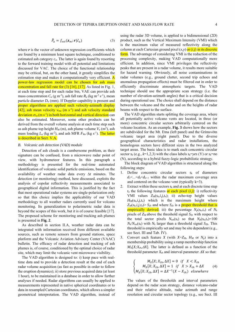
B. Volcanic ash detection (VAD) module
Detection of ash clouds is a cumbersome problem, as their
signature can be confused, from a microwave radar point of
view, with hydrometeor features. In this paragraph a
methodology is presented for the real-time automated
identification of volcanic solid particle emissions, based on the
availability of weather radar data every t minutes. The
detection (or monitoring) method, here discussed, exploits the
analysis of copolar reflectivity measurements associated to
geographical digital information. This is justified by the fact
that most operational radar systems are single-polarization only
so that this choice implies the applicability of our VAD
methodology to all weather radars currently used for volcano
monitoring. Its generalization to polarimetric radar data is
beyond the scopes of this work, but it is of course feasible [17].
The proposed scheme for monitoring and tracking ash plumes
is presented in Fig. 2.
As described in section II.A, weather radar data can be
integrated with information received from different available
sources, such as remote sensors from ground stations, space
platform and the Volcanic Aviation Advisory Center (VAAC)
bulletin. The efficacy of radar detection and tracking of ash
plumes is, of course, conditioned by the optimal choice of radar
site, which may limit the volcanic vent microwave visibility.
The VAD algorithm is designed to: i) keep pace with real-
time data and to provide a detection result at the end of each
radar volume acquisition (as fast as possible in order to follow
the eruption dynamics); ii) store previous acquired data (at least
1 hour), to be maintained in a database in order to allow further
analyses if needed. Radar algorithms can usually be applied to
measurements represented in native spherical coordinates or to
data in resampled Cartesian coordinates, which allows a simpler
geometrical interpretation. The VAD algorithm, instead of
using the radar 3D volume, is applied to a bidimensional (2D)
product, such as the Vertical Maximum Intensity (VMI) which
is the maximum value of measured reflectivity along the
column at each Cartesian ground pixel (x,y) or (i.j) in its discrete
form. The advantage of considering VMI is the reduction of the
processing complexity, making VAD computationally more
efficient. In addition, since VMI privileges the reflectivity
peaks that are present in a radar volume, it results more suitable
for hazard warning. Obviously, all noise contaminations in
radar volumes (e.g., ground clutter, second trip echoes and
anomalous propagation effects) must be filtered out in order to
efficiently discriminate atmospheric targets. The VAD
technique should use the appropriate scan strategy (i.e. the
number of elevation-azimuth angles) that is a critical decision
during operational use. The choice shall depend on the distance
between the volcano and the radar and on the heights of radar
beams with respect to the surface.
The VAD algorithm starts splitting the coverage area, where
all potentially active volcano vents are located, in three (or
more) concentric circular sectors arbitrarily centered on the
volcano location. As an example, Fig. 3 shows how the sectors
are subdivided for the Mt. Etna (left panel) and the Grímsvötn
volcanic target area (right panel). Due to the diverse
geographical characteristics and radar installations, the
homologous sectors have different sizes in the two analyzed
target areas. The basic idea is to mark each concentric circular
sector sk (e.g., k=1,2,3) with the class labels sk=yes (Y) or sk=no (N), according to a hybrid fuzzy-logic probabilistic strategy.
The block diagram of VAD algorithm is structured along the
following steps:
1. Define concentric circular sectors sk of diameters
d1<...<dk<dk+1 within the radar maximum coverage area
and centered on the volcano vent (typically k=3).
2. Extract within these sectors sk and at each discrete time step
tn the following features at each pixel (i.j): i) reflectivity
VMI values ZM(sk,i,j,tn); ii) echo-top height values
HM(sk,i,j,tn) which is the maximum height where
ZM(sk,i,j,tn)> SZk and where SZk is a proper threshold that is
empirically derived; iii) the percentage Np(sk,tn) of Nk
pixels of ZM above the threshold signal SZk with respect to
the total sector pixels Ntot(sk) so that Np(sk,tn)=100
Nk/Ntot(sk) with Nk larger than a threshold signal SZk. This
threshold is empirically set and may be site dependent (e.g.,
see Sect. III and Tab. IV).
3. Convert each feature X (with X=ZM, HM or Np) into a
membership probability using a ramp membership function
MX[X;Xth,X]. The latter is defined as a function of the
threshold parameter Xth and interval parameter X so that:
; , ∆ ; , ∆ ∆; , ∆ ∆ (4)
The values of the thresholds and interval parameters
depend on the radar scan strategy, distance volcano-radar
and their relative altitude, radar azimuth and range
resolution and circular sector topology (e.g., see Sect. III

DETECTION OF TEPHRA ERUPTION ONSET AND MASS FLOW RATE
5
and Table IV).
4. Define an inference rule function for each sector sk as the
product of the membership function of each feature X
(fuzzification stage): , , ; (5)
5. Assign a label “Y” (yes) or “N” (no) to each sector sk at
each time step tn, taking the maximum of the inference rule
function Ik and checking if it is greater or lesser than 0.5
(defuzzification stage)
, , , ; , → , → (6)
where the maximum Maxij is searched within all pixels (i,j) of sector k if the percentage number of pixels is above a
given threshold SNk that is typically empirically derived. 6. Estimate a probability of ash eruption (PAE) at a given
time step tn by evaluating different temporal combinations
for sk=Y or N at previous time steps tn-i (with i=1NV) as
follows (ash-eruption conditional probability stage): , | , ∆ , | , (7a)
with
, | ,∆ , | , , | , , | ,
(7b)
where pash(tn,s1=Y|s2,s3) and pash(tn-i,s1|s2,s3) are the ash
conditional probabilities, respectively, at present instant tn and at previous acquisition time steps tn-i for a given class
label combination in s1, s2 and s3, whereas NV is the number
of volumes considered in previous acquisition time steps
within the interval tn. PAE in (7) is the product of two
conditional probabilities of ash: the current probability of
ash when in the inner sector s1=Y and the temporal average
of past probabilities in sector s1, both conditioned to the
outcomes of (5) in outer sectors s2 and s3. Note that the PAE
value is computed automatically after every radar volume
scan and its value ranges from 0 to 1.
The time span tn of the average probability pavg is
typically set to 1 hour so that NV=tn/t with t the time
step of radar acquisition. Both pash(tn) and pash(tn-i) are
empirically tunable probabilities, depending on the
volcanic observation scenario and available information.
These conditional probabilities are meant to discriminate
ash plumes from meteorological storms exploiting their
different temporal evolution. As an example, from the
analysis of past case studies of volcanic eruptions in
Iceland and Italy, Table I and Table II provide,
respectively, the conditional current and previous
probability pash in (7), derived from label combinations in
sectors 2 and 3 and depending on the label (Y or N) of
sector 1. It is worth recalling that, if s1=N at current instant
tn, the PAE value is set to zero automatically. The proposed
values in the previous tables basically guarantee that
volcanic ash is not detected in cases of persistent and/or
widespread radar echoes, likely due to moving stratiform
meteorological storms covering the outer sectors in the
volcano surrounding. Convective rain clouds, developing
close to the volcano vent as in many tropical volcanoes,
might be confused with ash plumes. In this respect, radar
polarimetry could help in refining the detection procedure.
From our experience, for the Icelandic and Italian volcanic
eruption cases, PAE≥0.8 is associated to the presence of
ash plumes, whereas PAE≤0.6 are mainly due to
meteorological targets. On this basis, as soon as sector 1 is
labeled as Y, the PAE value is computed by means of (7).
7. Label the radar echoes around the potential volcanic vent
in the inner sector s1 at instant tn by means of LPAE(tn,s1),
defined as (ash-eruption target labeling stage): ,
(8)
where TE1 and TE2 are proper thresholds, typically set to
0.6 and 0.8 respectively as mentioned before.
8. The spatial identification of radar echoes, affected by ash,
can be performed by introducing the Probability of Ash
Detection (PAD). The latter is an areal probability of
detection applied to all pixels within radar coverage
estimated as (ash-detection conditional probability stage): , , ,, , ]
(9)
where the new membership function MD takes into account
the distance between the pixel (i,j) and the volcano vent.
Roughly speaking, (9) reveals the presence of ash in a given
pixel if there is a suitable distance from the vent via d, if those
pixels lie in a specified range of altitudes via HM and if the
maximum reflectivity is sufficiently high via ZM. PAD values
are in the same range of the PAE; in (9) the weights wz and
wH can be set to 0.5, but they can take into account the
instantaneous availability of each source of information and
its strength. The PAD formula in (9) may be enriched and
improved by exploiting additional radar features, such as
spatial texture and gradient of reflectivity, radial velocity as
well as some polarimetric features.
9. In similar fashion to (8), we can then define a radar
detection label LPAD(tn,i,j), which has generally different
thresholds TE3 and TE4. The LPAD label is introduced to
discriminate among meteorological and ash in each pixel
of the radar domain taking into account any uncertain or
mixed condition (ash-detection target labeling stage):
DETECTION OF TEPHRA ERUPTION ONSET AND MASS FLOW RATE
6
, ,
(10)
If LPAE(tn,s1)=”Ash”, the VAD algorithm switches
(automatically or semi-automatically) into a warning mode
so that tracking (VAT), classification (VAC) and estimation
(VAE) procedures can be activated. These modules are
applied to (i,j) pixels where PADk(i,j ,tn)≥ TE3, in order to
keep pixels labeled as ash or as uncertain. The probability
PAE in (7), immediately after the ash detection instant tn, must be evaluated with Table III, instead of Table I, in order
to verify if the volcanic ash eruption from the vent is a
continuing phenomenon.
If LPAE(tn,s1)=”Uncertain”, reflectivity echoes can be
affected by false alarm or misdetection due to mixed phase
(hydrometeor and ash signatures) or under particular
atmospheric conditions.
If LPAE(tn,s1)=”Meteorological”, VARR-chain successive
modules are not activated and the detection cycle is updated
to the next time step. Note that, if immediately after
LPAE(tn,s1)=”Ash”, then s1=N and PAE is set to zero and
probably a false alarm may have happened or it may behave
intermittently. On the other hand, if the eruption stops after
some time, dispersed ash will be detected only into outer
sectors but not in the inner sector s1. In these cases, VAT,
VAC and VAE are applied anyway to (i,j) pixels where
PAD(i,j ,tn)≥ TE3.
In summary, the probability of the volcanic eruption onset is
described in time by the PAE time series evolution. Its behavior
is an indicator of eruption column ejecting ash in the
surrounding of the volcanic vent. On the other hand, the spatial
discrimination between ash and meteorological radar echoes is
performed by PAD maps. The efficiency of the latter is, of
course, essential for any prompt and effective support to
decision.
III. RADAR-BASED DETECTION OF VOLCANIC ERUPTION ONSET
The VAD algorithm has been tested for several volcanic
eruptions and requires that a weather radar is available and
operating during the eruption, which is not always the case
when eruptions occur.
As an example, here we will show the results obtained from
the volcanic eruption that occurred on May 2011 at the
Grímsvötn volcano, located in the northwest of the Vatnajökull
glacier in south-east Iceland (e.g., [27]). It is one of the most
active Icelandic volcanoes. An explosive subglacial volcanic
eruption started in the Grímsvötn caldera around 19:00 UTC on
May 21, 2011. The strength of the eruption decreased rapidly
and the plume was below ~10 km altitude after 24 h [40]. The
eruption was officially declared over on 28 May at 07:00 UTC.
More details on the Grímsvötn eruption observations and
estimates can be found in [27] and [23] with a comprehensive
analysis of the eruptive event from VAC and VAE results using
polarimetric radar data at X band.
The X-band dual polarization radar measurements (DPX)
used in this study are acquired by the Meteor 50DX system
which is a mobile compact weather radar deployed on a
transportable trailer. For the volcanic event of May 2011 in
Iceland, it has been positioned in the Kirkjubæjarklaustur,
southern Iceland, at approximately 75 km from the Grímsvötn
volcano [23]. During its operational activities on May 2011,
DPX scans were set to 14 elevations angles from 0.7° to 40°.
All polarimetric observables have a range, azimuth and time
sampling of 0.20 km and 1° and 10 min, respectively and have
been properly post-processed to remove ground-clutter and
others impairments. A flow diagram of the VARR algorithm
chain is shown in Fig.4. The data processing steps, applied to
this case study and here summarized, are well described in [23].
Three concentric circular sectors, centered at the Grímsvötn
eruption vent have been set up having a maximum range of 8,
20 and 60 km respectively (see Fig. 3, right panel). The number
of time steps NV, to be used in (7), depends on the rate of radar
scans; since in this case scans are every 10 minutes, then NV=6
within an hour. Results of VAD for this case study are shown
in Fig. 5 and Fig. 6 on 2 time intervals on the third day, as an
example. PAE values have been computed using the processing
chain of Sect. II since the beginning of eruption in different
weather condition. The label value (Y” or “N”) of each sector
is also shown for completeness. The maximum values of the
detected reflectivity, along the vertical column centered on (i,j), are projected on the surface as a Plan Position Indicator (PPI)
georeferenced radial map. The label VMI-CZ in these figures
stands for vertical maximum intensity corrected reflectivity
where the corrections are those usually related to ground-clutter
removal and Doppler dealiasing [42].
The ash plume is visible over the Grímsvötn volcano,
especially looking at the sequence of Fig. 5 where strong
reflectivity values are detected around the vent in clear air
conditions. On the contrary, Fig. 6 shows the sequence of PAE
values in presence of a small horizontally-extended ash plume
coexisting with other meteorological clouds in the outer sectors.
The latter may cause false alarms, but the conditional check of
all sectors avoids apparent detection errors. The detected
volcanic plume is also distinguishable from undesired residual
ground clutter returns, the latter being recognizable as it tends
to show a VMI stationary field from an image to another.
The temporal sequence of PAE, which might represent an
operational warning product of VAD, is shown in Fig. 7 for
whole days of 24 and 25 May. In this figure gray areas indicate
the instants where we have found an ash plume by visual
inspection of each radar scan. The colored circles in the PAD
sequence refer to hit, false and miss plume detection. The hit
rate (green circles) is high and this is an encouraging result for
further tests. In the case of 2011 Grímsvötn event the observed
temporal sequence definitely indicates a distinct ash feature
erupted from the volcano vent, which can be effectively
detected by means of the PAE product. Missed detection (i.e.,
observed, but not detected by PAE algorithm) is due to very low
reflectivity values around the volcano vent correlated to the
small observed plume. False detection could instead occur
when rain clouds, developing close to the volcano vent, are
DETECTION OF TEPHRA ERUPTION ONSET AND MASS FLOW RATE
7
confused with ash plumes.
Some examples of PAD results, computed by (9), are shown
in Fig. 8 for some instants selected considering different
weather conditions. The results are expressed using the radar
detection label LPAD, in (10), once setting the thresholds TE3=0.6
and TE4=0.8. As expected, in case of an ash eruption in clear air
with strong reflectivity values, as in May 23, 12.21 UTC, the
PAD is set to ash mode. In the mixed scenario of May 23, 13.30
UTC PAD changes into uncertain mode; it is worth noting that
the residual ground clutter is classified as a meteorological
target, as expected.
IV. RADAR AND INFRASOUND DETECTION OF ASH
MW weather radars can scan the whole atmosphere in a 3D
fashion in an area of about 105 km2 [12]. The entire volume is
accomplished in about 3 to 5 minutes depending on the number
of elevation angles, azimuth angles and range bins, but also on
the antenna rotation rate (which is typically of 3 to 6 rounds per
minutes). This means a single voxel (volume pixel) of the 3D
volume can only be sampled every few minutes. In this respect
MW weather radar can benefit from the integration of other
volcanic site measurements with a more rapid sampling, but
still sensitive to the onset of the ash eruption. This paragraph
will explore this synergetic scenario.
The Mt. Etna volcano (Sicily, Italy) has produced more than
fifty lava fountains since 2011 from a new crater formed in
November 2009 [25], [18]. These events are characterized by
the onset of Strombolian activity accompanied by volcanic
tremor (resumption phase), an intensification of the explosions
with the formation of an eruption column producing ash fallout
(paroxysmal phase) and, finally, the decrease of both the
explosion intensity and volcanic tremor (final phase) ([20],
[25]).
The Mt. Etna eruption of Nov. 23, 2013 was a lava fountain
event more intense than usual which began in the afternoon of
November 22, intensified after 07:00 UTC of Nov. 23 [26]. The
lava fountain formed at 09:30 UTC and lasted up to 10:20 UTC,
forming a magma jet up to about 1 km and an eruption plume
higher than 9 km that dispersed volcanic ash toward the north-
eastern volcano flanks [35]. The eruption ended at about 11:30
UTC.
This Mt. Etna eruption was observed by the same DPX X-
band radar system, deployed in Iceland in 2011 (see Set. III). In
this case the DPX radar is permanently positioned at the Catania
airport (Sicily, Italy) at an altitude of 14 m and approximately
32 km far away from the Mt. Etna crater of interest (see Fig 3a,
left panel). The DPX radar system works at 9.4 GHz and is
operated to cover an area within a circle of 160 km radius every
10 minutes [23]. Fig. 9 shows temporal samples of VMI
imagery showing the onset of the lava fountain at 9:40 UTC,
the intensification and the dissipation around 10:40 UTC. Note
that the ash plume is not detected by DPX radar after 10:40
UTC since radar is not sensitive to fine ash (with sizes less than
about 50-micron diameter) at long range which is indeed
dispersed in the north-east direction after the eruption end.
Volcanic activity produces infrasonic waves (i.e. acoustic
waves below 20 Hz), which can propagate in the atmosphere
useful for the remote monitoring of volcanic activity [20].
Infrasound (IS) associated with explosive eruptions is generally
produced by the rapid expansion of the gas–particle mixture
within the conduit and, in consequence, it is related to the
dynamics of the volume outflow and thus to the intensity of the
eruption [21], [22]. At Mt. Etna a 4-element IS array (with small
aperture of 120-250 m, at an elevation of 2010 m above sea
level and at a distance of 5500m from the summit craters) has
been operating since 2007 [25]. Each element has a differential
pressure transducer with sensitivity of 25 mV/Pa in the
frequency band 0.01–50 Hz and a noise level of 10-2 Pa. Array
analysis is performed by a multichannel semblance grid-
searching procedure using a sliding 5-s long window. The
expected azimuth resolution is of ~2°, which corresponds to
about 190m at a distance of 5.5 km. The IS array mean pressure
amplitude PISmean of the acoustic signals detected by the array in
5 min long time window is usually computed for data analysis.
Details on this installation, operating as part of the permanent
monitoring system of Etna volcano, can be found in [25].
Similarly to Fig. 7, Fig. 10 and Fig. 11 show the time series
of estimated probability of ash eruption and plume maximum
height above the sea level, respectively, derived from the VAD
algorithm during the Mt. Etna eruption of Nov. 23, 2013.
Instantaneous mean pressure from infrasonic array, sampled
every 5 seconds, is also superimposed for the same event. The
interesting feature, noted in Fig. 10, is the time shift between
the MW radar detection and infrasound signature. In particular,
in this case the time difference between radar-based maximum
height HM and infrasound-based PISmean peak is about 17 min,
the VAE-based maximum plume height above the vent is about
7.9 km, the horizontal distance up to HM peak from vent is about
12 km.
This time shift between MW radar and PISmean infrasound is
due to the time necessary for the plume to reach its maximum
height, and, therefore, is related to the plume rising velocity.
Nonetheless, while infrasound is peaking the increase of
pressure at the vent, the radar is detecting the MW maximum
values above the vent. Using data shown in Fig. 10 and 11, we
can thus estimate the average uprising velocity of the erupted
mixture: the vertical component is about 7.7 m/s whereas the
horizontal component is about 11.7 m/s. These estimates seem
to be consistent with a buoyancy-driven ascent for volcanic
plumes such as that on Nov. 23. In summary, this investigation
seems to confirm that: i) combination of radar and IS data are
ideal ingredients for an automatic ash eruption onset early
warning within a supersite integrated system (see Fig. 1); ii) the
shift between MW radar and IS array signatures may provide
estimate of the mean buoyant plume velocity field.
V. MASS FLOW RATE ESTIMATION AT THE VOLCANO VENT
Once the eruption onset is detected by VAD and tracked by
VAT, in order to forecast the ash dispersal, it is fundamental to
estimate the source mass flow rate at the volcano vent [28]. The
plume maximum height, the vertical distribution of erupted
mass and the rate of ash injection into the atmosphere, all
depend on the MFR, wind entrainment and advection,
temperature of the erupted mixture and the atmospheric
DETECTION OF TEPHRA ERUPTION ONSET AND MASS FLOW RATE
8
stratification [4]. In this respect, both MW radar and infrasound
measurements can help and in this section we will compare
them with estimates from a parametric analytical model using
data of the 2010 of Eyjafjallajökull, eruption [30].
During the eruption in April-May 2010 of Eyjafjallajökull
stratovolcano, the ash plume was monitored by a C-band
scanning weather radar, managed by IMO (Icelandic
Meteorological Office) and located in Keflavik at 155 km from
the volcano [14], [15]. The single-polarization Keflavik radar
provides the reflectivity factor Zhhm every 5 minutes. By
applying the VAC and VAE of the VARR algorithm (see Fig.
1), we have obtained the ash concentration estimates for each
radar bin considered above the volcano vent. The trend of the
plume top height shows values between 5 and 6 km above sea
level in agreement with other observations [14], [15].
A. Radar-based and infrasonic retrieval of source MFR
These VAE-based ash concentration estimates have been
used to provide an approximate quantification of source MFR
at the vent [31]. The evolution of a turbulent plume formed
above the vent during an explosive eruption can be described
physically by mass conservation equation within a volume
above the vent. By integrating over the columnar volume Vc
within the closed surface Sc above the vent and using the
divergence theorem, we can obtain the radar-based source MFR
FRrad (kg/s) defined as sum of derivative mass rate DR (kg/s) and
the mass advection rate AR (kg/s) [31]:
(11a)
where, if r=[x,y,z] is the position vector, n0 is the outward
normal unit vector and va is the ash mass velocity field, it holds:
,, ∙ , (11b)
where Sc is the surface enclosing the volume Vc wher the mass
balance is computed.
By discretizing (11), source MFR can be estimated from
weather radar measurements around the volcano vent, imposing
the time step ∆t equal to the radar scan sampling time (here, 5
minutes) and setting up the horizontal section of the columnar
volume VC (here, 5x5 pixels with a pixel size of about 1 km per
side). The 3D vectorial velocity field va(r ,t) of the divergent
advection rate AR can be estimated either from radar Doppler
moments (if available) or from temporal cross-correlation
techniques, such as PCORR (see Sect. II), applied in a 3D
fashion. If the advection rate is neglected, then MFR is
underestimated as advective outflow tends to remove ash from
the column.
MFR can be estimated by means of infrasonic array
measurements [19]-[21]. In the far-field conditions (i.e. for
acoustic wavelength much larger than source dimension), the
linear theory of sound demonstrates that acoustic pressure can
be related to the source outflow velocity assuming a monopole,
dipole or quadrupole source of sound [34]. Thermal camera
imagery suggested that the sound associated with the
Eyjafjallajökull ash plume dynamics is more consistent with the
dipole source [19]. Under the assumption that the acoustic
velocity of the expanding surface within the conduit is
equivalent to the plume exit velocity (as suggested by thermal
imagery analysis of Strombolian explosions [43]), for a
cylindrical conduit of radius Rv, the infrasound-based source
MFR FRifs can be calculated as [19]:
. ∙ ∙ . ∙ / (12)
where Rv is the estimated radius of the vent, p is the mixture
density, PISmean is the mean pressure amplitude, air is the
density of the atmosphere, c the sound speed and rs is the
distance from the source (see [19] for parameter values). For
this case study, the ash plume activity of Eyjafjallajökull in
2010 has been recorded using a 4-element infrasonic array at a
distance of 8.3 km from the craters. These sensors were chosen
for their wide frequency band, good pressure sensitivity, and
low power requirement (about 60 mW). All the array elements
were connected to the central station by cables and data were
digitized and transmitted via Internet link to the Icelandic
Meteorological Office (IMO).
B. Analytical and model-based evaluation of source MFR
Another way to estimate MFR from the eruptive plume top
height is to resort to simplified parametric empirical formulas
(e.g., [4], [6], [36]) and analytical equations (e.g., [28]). In
particular, HM can be derived from radar scans (even though the
finer particles in the upper plume can be missed due to reduced
sensitivity) [14], [15], [38]. The source MFR of a volcanic
plume is fundamentally related to the plume top height as a
result of the dynamics of buoyant plume rise in the atmosphere,
but is also affected by atmosphere stratification (buoyancy
frequency), cross-wind and humidity [28], [33]. A nonlinear
parametric equation to estimate FRmod has been derived, to
include both local cross-wind and buoyancy frequency
conditions at a given instant [28]:
(13)
where a0, a1 and a2 are coefficients dependent on the
gravitational acceleration, air and plume density, air and plume
temperature, specific heat capacity of both air and particles,
buoyancy frequency, radial entrainment, wind entrainment and
wind velocity profile. The application of (13) (from now on
defined as D&B analytical model) at given time step t requires
that the atmospheric conditions close to the volcanic vent are
known in order to evaluate the plume bending under the wind
effects. Under the approximation of horizontal uniformity of
free troposphere, these conditions can be derived from the
closest radiosounding (RaOb) station. For this case study
atmospheric conditions obtained by ECMWF ERA-40
reanalysis at 0.25° resolution interpolated above the
Eyjafjallajökull volcano (see Fig. S5 in [28]). The other
parameters used in (13) are listed in Table S1 and S2 of [28].
The source MFR, here labelled as FRnum(t), can also be
derived from one-dimensional (1D) numerical models, [28].
The latter are based on the theory of turbulent gravitational
DETECTION OF TEPHRA ERUPTION ONSET AND MASS FLOW RATE
9
convection from a maintained volcanic source taking into
account wind and humidity in the atmosphere, based on
Morton’s theory [37]. Results from 1D numerical models are
can be obtained by Monte Carlo simulations run over a large
parameter space of source conditions (temperature, exit
velocity, exsolved gas mass fraction, vent radius, vent height),
atmospheric conditions (temperature, wind, and humidity
profiles), and radial and wind entrainment coefficients [28].From this ensemble of 1D Monte Carlo simulation a minimum
and maximum value ofFRnum(t) can be derived at each time step.
For these simulations we used the same parameters and
atmospheric conditions as in (13), but also take into account the
humidity atmosphere (see Fig. S5 in [28]). The source
conditions used can be found in Table S2 in [28].
C. Intercomparison results
The temporal trend of the VARR-based MFR FRrad(t), for
the period of May 5-10, 2010, is shown in Fig. 12 by comparing
FRrad(t) obtained with and without the advection term in (11a)
at 10-minute sampling as well as every half hour, 1 hour and 3
hours. The MFR variability, as detected and estimated by the
weather radar, shows a pulsed behavior of the MFR at shorter
time scales [31]-[32]. Note that the oscillations of VARR-based
MFR estimates may be affected by the time sampling of the
radar and the volume scan time interval, which is accomplished
in a few minutes, whereas the ash plume parameters can vary
on the order of a few seconds.
Neglecting the advection term in (10) may lead to a MFR
underestimation on average less than an order of magnitude or,
in terms of percentage fractional difference, larger than 100%
(see middle panel of Fig. 12). This VARR-derived MFR
variability is about two order of magnitudes at 10-minute
sampling and about an order of magnitude after 1-hour
averaging with a mean value around 5 105 kg/s within the
observed period. The radar-based capability to catch the MFR
intermittent behavior is, to a certain extent, expected as it
closely correlates with the pulsating explosive activity through
the estimate of the ash mass change and advection [32]. It is
worth noting that MFR estimates from field data during the
period between 4 and 8 May have provided average values
between 0.6 and 2.5 105 kg/s [28], [30], not too far from VARR-
based MFR variability around its mean value (see Fig. 12).
VARR-based MFR values are also higher than those estimated
by near-field video analyses between 2.2 and 3.5 104 kg/s [36],
but closer to those derives from other plume height models
between 26.2 and 43.6 104 kg/s [36], [33].
Fig. 13 shows MFR temporal trends in terms of the minimum
and maximum values of FRnum(t), derived from the Monte Carlo
1D numerical model using radiosonde available every hour,
compared to the minimum and maximum values of FRrad(t), derived from VARR-based algorithm taking every 10 minutes
within a running window of 60 minutes. The average value of
1D-model MFR is about 105 kg/s within the observed period,
whereas minimum values are cut at 102 kg/s, lower values
indicating that there were significant humidity effects. This
only affects the minimum MFR estimate. The peak-to-peak
variability of VARR-derived estimates of MFR is typically
between 104 and 106 kg/s with episodes down to 103 kg/s
between around May 9. Radar-based MFR tends to be larger
than that exhibited by the 1D numerical model, except in a few
cases where the 1D model shows much lower minimum values.
These low values can be, for the most part, attributed to the
strong humidity effects in the period after May 8, 2010. Due to
the change in heat capacity and latent heat release associated
with condensation, even plumes with very low mass flow rates
can obtain the observed heights [28]. Additionally, there is a
larger variability of the plume tops in this period, whose
minimum values tend to be much lower than those before May
8.
Fig. 13 also shows the intercomparison among the 1-hour
sampled temporal trends of FRrad(t), FRmod(t) and FRifs(t), that is,
respectively, MFR estimates obtained from the VARR radar
algorithm (expressed as a 1-hour average together with its
standard deviation), from the D&B analytical model, (i.e. using
(13) applied to the minimum and maximum radar-retrieved
plume height every hour; see [28] for details), from the 1D
numerical model and from infrasonic array data. Both MFR
estimates VARR radar and infrasound estimates of averaged
MFR are in quite good agreement being the infrasound estimate
within the standard deviation of radar-based MFR around 106
kg/s. The D&B analytical model tends to provide a lower MFR
especially after May 8, 2010. This behavior is strictly linked to
the radar estimate of the plume top height HM in (13), which
tends to be lower in the observation period [29], [14], [15].
Indeed, radar estimates of HM may be an underestimation of the
true plume top height due to the reduced sensitivity to particles
size finer than 50 microns and to the possible occlusions of
observation sectors due to ground clutter.
It is also worth noting that, even at the same time sampling
of 1 hour, VARR-based estimates of source MFR exhibit a
higher intermittency with respect to 1D-model and infrasound
estimates with a MFR variability larger than one order of
magnitude (this variability is increased up to 2 order of
magnitudes at 10-minute sampling in Fig. 12). This feature,
which should be confirmed by future investigations, might be
related to the fact that the VARR-derived MFR is strictly linked
to the mass change rate and its advection, whereas 1D-model
estimates depend on the plume top height (which may respond
in a slower source flux changes) and infrasound estimates are
indirectly correlated to the source MFR through the measured
acoustic wave pressure. Furthermore, the uncertainty in the
observed parameters of these methods is amplified by the
uncertainty of the model parameters used in (12), (13), and the
1D model. In the case of the 1D plume model and the analytical
expression (13), for example, the results can be very sensitive
to the choice of entrainment coefficients [44].
VI. CONCLUSION
A hybrid algorithm, named VAD that exploits weather radar
data, has been presented to detect the onset of the explosive
volcanic eruption and estimate the mass flow rate at the volcano
vent. The VAD approach, part of the VARR methodology, can
provide the probability of ash detection (PAD) within the radar
coverage area and the probability of ash eruption (PAE) at the
fissure. Estimates of PAE have been provided for two eruption
case studies, in Iceland on 2011 and in Italy in 2013. The
quantitative analysis show very encouraging results in terms of
detection and labeling which can be useful for any support
decision system dealing with volcanic eruption hazard. The
DETECTION OF TEPHRA ERUPTION ONSET AND MASS FLOW RATE
10
PAE index can be usefully exploited as a diagnostic tool for an
early warning integrated platform, which can be of interest for
civil prevention and protection. Assuming to pursue a self-
consistent radar approach, a way to improve PAE is to also
exploit in case of uncertain labeling: i) spatial texture of ash
field radar observables versus rain field around the volcano
vent; ii) temporal evolution of the radar observables around the
volcano vent; iii) Doppler spectrum (mean and spectral width)
variability in time and space around the volcano vent; iv)
vertical section (RHI) of measured reflectivity along the radar-
vent cross section; v) detection of a strong reflectivity gradient
(both in space and time) due to ash cloud; vi) use of some
polarimetric observables, such as Zdr, since for tumbling ash
particles Zdr≈0 for any concentration and diameter, whereas for
strong reflectivity ash may have Kdp values near or less than
zero as opposed to rainfall. Correlation coefficient should have
low values above and around volcano vent in case of eruption
being a great mixture of non-spherical particles.
This work has also explored, using the Italian case study in
2013, the synergy between microwave weather radars and
infrasonic array observations. The latter have been already used
for detecting Etna lava fountains with a high degree of
confidence thus demonstrating to be an essential tool for
volcanic eruption early warning. Before designing an integrated
tool, the interpretation of the respective signatures needs to be
investigated and this has been the goal of the presented analysis.
Results indicate that the response of the weather radar and
infrasonic array to the eruption onset of the plume is correlated
and characterized by a time lapse due to the plume rise. The
different time sampling of the 2 measurements, typically 10 and
1 minute for radar and infrasound respectively, should be taken
into consideration when trying to derive eruption dynamical
parameters. If confirmed by further case analyses, the synergy
of weather radar and infrasonic array can be framed within the
VAD hybrid algorithm by introducing a proper conditional
probability of PAE driven by infrasonic array data. This may
help VAD to remove ambiguous mixed-phase conditions where
the ash plume is coexisting with the meteorological clouds.
Finally, VARR-based retrievals of the source MFR at the
vent have been analyzed for a further event in Iceland in 2010
by comparing with estimates of a 1D numerical model, an
analytical formula and infrasonic array data. The estimate of
source MFR is considered a fundamental step to characterize
the volcanic source, but very difficult to measure accurately.
Thus, this work for the first time has proposed the
intercomparison between 2 experimental techniques, based on
weather radar and infrasonic array data, supported by the
analyses of 2 modeling approaches. The results show a
substantial agreement about the average estimate of MFR from
both instruments with the VARR-based showing a larger
variability probably due to the source pulse intermittency. The
1D-model variability is within the peak-to-peak estimate of
VARR, whereas the wind-driven analytical model can
underestimate MFR due to the limits in the estimation of top
plume height by radar. Five minutes time resolution appears to
be a good compromise to estimate 1-h average mass flow rate
and its standard deviation and to allow a complete volume radar
scan.
Further work is required to assess the usefulness of VAD on
a statistical basis using a significant number of case studies as
well as to couple it with collocated infrasonic array pressure
measurements. Unfortunately, only few volcanic sites are
nowadays equipped with both instruments and the historical
dataset is very limited so far. The probability of ash eruption
value and relative spatial identification by means of synergetic
PAE and PAD values can be displayed continuously on a
devoted web site. Positions of potentially active volcanoes
should be displayed as an overlay on monitoring screens.
Seismic data can complement the VARR scheme as a priori
data in the VAD radar detection module. We expect them to be
less correlated to the eruption onset, but they can corroborate
and increase the VAD probability of detection. L-Band Doppler
radar monitoring with a fixed beam aiming near the source can
be easily ingested in the detection procedure (an example can
be the Voldorad L-band system near the Etna volcano). Other
data, coming from ground-based and space-based remote
sensors, can be also combined within VARR in order to provide
a comprehensive quantitative overview of the evolving eruption
scenario and its source parameters, useful for supporting the
decisions of the interested Volcanic Ash Advisory Center.
ACKNOWLEDGMENT
We are very grateful to B. Pálmason, H. Pétursson and S.
Karlsdóttir (IMO, Iceland) for providing X and C-band Iceland
radar data and G. Vulpiani and P. Pagliara (DPC, Italy) for
providing X-band Italian radar data. The application of VARR
chain algorithms, developed in C language and Matlab®
environment, can be discussed with the authors upon request.
REFERENCES
[1]. Miller, T.P., Casadevall, T.J., Volcanic ash hazards to aviation. In:
Sigurdsson, H., Houghton, B.F., McNutt, S.R., Rymer, H., Stix, J. (Eds.),
Encyclopedia of Volcanoes. Academic Press, San Diego, pp. 915–930,
2000.
[2]. O’Regan, M., On the edge of chaos: European aviation and disrupted
mobilities. Mobilities 6 (1), 21–30, 2011.
[3]. Prata, A.J. and Tupper, A., Aviation hazards from volcanoes: the state of
the science,. Nat. Hazards, 2009. http://dx.doi.org/10.1007/s11069-009-
9415-y.
[4]. Sparks, R. S. J., Bursik, M. I., Carey, S. N., Gilbert, J. S., Glaze, L.,
Sigurdsson, H., and Woods, A.W., Volcanic plumes. New York, Wiley,
1997.
[5]. Stohl, A., Prata, A. J., Eckhardt, S., Clarisse, L., Durant, A., Henne, S.,
Kristiansen, N. I., Minikin, A., Schumann, U., Seibert, P., Stebel, K.,
Thomas, H. E., Thorsteinsson, T., Tørseth, K., and Weinzierl, B.,
“Determination of time- and height-resolved volcanic ash emissions and
their use for quantitative ash dispersion modeling: the 2010
Eyjafjallajökull eruption”, Atmos. Chem. Phys., vol. 11, pp. 4333–4351,
doi:10.5194/acp-11-4333-2011, 2011.
[6]. Mastin, L.G., Guffanti, M., Servranckx, R., Webley, P., Barsotti, S., Dean, K., Durant, A., Ewert, J.W., Neri, A., Rose, W.I., Schneider, D., Siebert, L., Stunder, B., Swanson, G., Tupper, A., Volentik, A., Waythomas, C.F, “A multidisciplinary effort to assign realistic source parameters to models of volcanic ash-cloud transport and dispersion during eruptions”. J Volcanol. Geoth. Res. vol. 186, pp. 10-21, 2009.
[7]. Rose W.I., G. J. S. Bluth, and G. G. J. Ernst, “Integrating retrievals of volcanic cloud characteristics from satellite remote sensors: A summary”, Philos. Trans. Roy. Soc. London, A358, 1538–1606, 2000.
DETECTION OF TEPHRA ERUPTION ONSET AND MASS FLOW RATE
11
[8]. Prata, A. J. and Grant, I. F.: Retrieval of microphysical and morphological properties of volcanic ash plumes from satellite data: Application to Mt. Ruapehu, New Zealand, Q. J. Roy. Meteorol. Soc., 127, 2153–2179, 2001.
[9]. Pavolonis, M. J.,Wayne, F. F., Heidinger, A. K., and Gallina, G. M.:A daytime complement to the reverse absorption technique for improved automated detection of volcanic ash, J. Atmos. Ocea. Technol., 23, 1422–1444, 2006.
[10]. Harris, D. M, and W. I. Rose, “Estimating particle sizes, concentrations, and total mass of ash in volcanic clouds using weather radar”. J. Geophys. Res., vol. 88, C15, pp. 10969–10983, 1983.
[11]. Lacasse, C., S. Karlsdóttir, G. Larsen, H. Soosalu, W. I. Rose, and G. G.
J. Ernst, “Weather radar observations of the Hekla 2000 eruption cloud”,
Iceland. Bull. Volcanol., vol. 66, 5, pp. 457–473, 2004.
[12]. Marzano F.S., E. Picciotti, G. Vulpiani and M. Montopoli, "Inside Volcanic clouds: Remote Sensing of Ash Plumes Using Microwave Weather Radars", Bullettin Am. Met. Soc. (BAMS), pp. 1567-1586, DOI: 10.1175/BAMS-D-11-00160.1, October 2013
[13]. Marzano, F.S., S. Barbieri, E. Picciotti and S. Karlsdóttir, Monitoring sub-
glacial volcanic eruption using C-band radar imagery. IEEE Trans. Geosci. Rem. Sensing, 48, 1, 403-414, 2010.
[14]. Marzano, F. S., M. Lamantea, M. Montopoli, S. Di Fabio and E. Picciotti,
The Eyjafjallajökull explosive volcanic eruption from a microwave
weather radar perspective, Atmos. Chem. Phys., 11, 9503-9518, 2011.
[15]. Arason, P., Petersen G. N. and Bjornsson H., Observations of the altitude
of the volcanic plume during the eruption of Eyjafjallajökull, April-May
2010, Earth Syst. Sci Data 3, 9-17, 2011.
[16]. Marzano, F. S., S. Barbieri, G. Vulpiani and W. I. Rose, “Volcanic ash
cloud retrieval by ground-based microwave weather radar”. IEEE Trans. Geosci. Rem. Sens., vol. 44, pp. 3235-3246, 2006.
[17]. Marzano F.S., E. Picciotti, G. Vulpiani and M. Montopoli, “Synthetic
Signatures of Volcanic Ash Cloud Particles from X-band Dual-
Polarization Radar”, IEEE Trans. Geosci. Rem. Sens., vol. 50, pp. 193-
211, 2012.
[18]. Scollo, S., Prestifilippo, M., Spata, G., Agostino, M.D, Coltelli, M.,
Monitoring and forecasting Etna volcanic plumes, Nat. Hazards Earth Syst. Sci. 9, 1573–1585, 2009.
[19]. Ripepe, M., Bonadonna C., Folch A., Delle Donne D., Lacanna G. and
Voight B., Ash-plume dynamics and eruption source parameters by
infrasound and thermal imagery: the 2010 Eyjafjallajokull eruption, Earth and Planetary Science Letters 366, 112-121, 2013.
http://dx.doi.org/10.1016/j.epsl.2013.02.005.
[20]. Jeffrey, B., Jonson, Aster R. C. and Kyle P.R., Volcanic eruptions
observed with infrasound, Geophysical Research Letters, Vol.31,
L14604, doi: 10.1029/2004GL020020, 2004.
[21]. Caplan-Auerbach, J., Bellesiles A. and Fernandes J. K., Estimates of
eruption velocity and plume height from infrasonic recordings of the 2006
eruption of Augustine Volcano Alaska, Journal of Volcanology and Geothermal Research, 2009. doi: 10.1016/j.jvolgeores. 2009.10.002.
[22]. Ripepe, M., De Angelis S., Lacanna G. and Voight B., Observation of
infrasonic and gravity waves at Soufrière Hills Volcano, Monserrat,
Geophysical Research Letters, Vol. 37, L00E14, doi:
10.1029/2010GL042557, 2010.
[23]. Montopoli M., G. Vulpiani, D. Cimini, E. Picciotti, and F.S. Marzano,
“Interpretation of observed microwave signatures from ground dual
polarization radar and space multi frequency radiometer for the 2011
Grímsvötn volcanic eruption”, Atmos. Meas. Tech.., ISSN: 1867-1381,
vol. 7, pp. 7, 537–552, 2014.
[24]. Marzano F.S., M. Lamantea, M. Montopoli, B. Oddsson and M.T.
Gudmundsson, “Validating sub-glacial volcanic eruption using ground-
based C-band radar imagery”, IEEE Trans. Geosci. Rem. Sens., ISSN:
0196-2892, vol. 50, pp. 1266-1282, 2012.
[25]. Ulivieri G., M. Ripepe, and E. Marchetti, “Infrasound reveals transition
to oscillatory discharge regime during lava fountaining: Implication for
early warning”, Geophysical Research Letters, VOL. 40, 1–6,
doi:10.1002/grl.50592, 2013.
[26]. Corradini S., M. Montopoli , L. Guerrieri, M. Ricci, S. Scollo, L. Merucci,
F.S. Marzano, S. Pugnaghi, M. Prestifilippo, L. Ventress, R.G. Grainger,
E. Carboni, G. Vulpiani, M. Coltelli, “A multi-sensor approach for the
volcanic ash cloud retrievals and eruption characterization”, Rem. Sensing, under review, 2015.
[27]. Marzano, F.S., M. Lamantea, M. Montopoli, M. Herzog, H. Graf, and D.
Cimini, “Microwave remote sensing of the 2011 Plinian eruption of the
Grímsvötn Icelandic volcano”, Remote Sens. Environ., vol. 129, pp. 168–
184, 2013.
[28]. Degruyter, W. and Bonadonna C., Improving on mass flow rate estimates
of volcanic eruptions, Geophysical Res. Lett., Vol.39, L16308, doi:
10.1029/2012GL052566, 2012.
[29]. Bjornsson, H., Magnusson S, Arason P, Petersen G.N., 2013 Velocities in the plume of the 2010 Eyjafjallajökull eruption. J Geophys Res Atmos 118:1–14. doi:10.1002/jgrd.50876.
[30]. Bonadonna, C., Genco R., Gouhier M., Pistolesi M., Cioni R., Alfano F.,
Hoskuldsson A. and Ripepe M., Tephra sedimentation during the 2010
Eyjafjallajokull eruption (Iceland) from deposit, radar, and satellite
observations, J. Geophys. Res., VOL. 116, B12202, doi:
10.1029/2011JB008462, 2011.
[31]. L. Mereu , Marzano, F.S. ; Montopoli, M. ; Bonadonna, C., “Retrieval of
Tephra Size Spectra and Mass Flow Rate From C-Band Radar During the
2010 Eyjafjallajökull Eruption, Iceland”, IEEE Trans. Geosci. Rem. Sens., pp. 5644-5660, 2015.
[32]. Kaminski, E., Tait S., Ferrucci F., Martet M., Hirn B. and Husson P.,
Estimation of ash injection in the atmosphere by basaltic volcanic plumes:
the case of the Eyjafjallajokull 2010 eruption, Journal Of Geophysical Research, Vol. 116, B00C02, doi: 10.1029/2011JB008297, 2011.
[33]. Woodhouse, M.J., A.J. Hogg, J.C. Phillips and R.S.J. Sparks, “Interaction
between volcanic plumes and wind during the 2010 Eyjafjallajo¨kull
eruption, Iceland”, J. Geophys. Res. Solid Earth, 118, 92–109,
doi:10.1029/2012JB009592, 2013.
[34]. Lighthill, M.J., Waves in Fluids. Cambridge University Press, New York,
pp.504, 1978.
[35]. Andronico D., S. Scollo, A. Cristaldi , “Unexpected hazards from tephra
fallouts at Mt Etna: The 23 November 2013 lava fountain”, Journal of Volcanology and Geothermal Research, vol. 304, pp. 118-125, 2015.
[36]. Dürig T., M.T. Gudmundsson, S. Karmann, B. Zimanowski, P. Dellino,
M. Rietze and R. Büttner, “Mass eruption rates in pulsating eruptions
estimated from video analysis of the gas thrust-buoyancy transition—a
case study of the 2010 eruption of Eyjafjallajökull, Iceland”, Earth, Planets and Space, vol. 67:180, DOI 10.1186/s40623-015-0351-7, 2015.
[37]. Morton, B. R., G. T. Taylor, and J. S. Turner, “Turbulent gravitational
convection from maintained and instanteneous sources”, Proc. R. Soc. London, Ser. A, vol. 234, pp. 1–23, 1956.
[38]. Oddsson B., Gudmundsson, M. T., Larsen, G., and Karlsdóttir, S.,
“Monitoring of the plume from the basaltic phreatomagmatic 2004
Grímsvötn eruption—application of weather radar and comparison with
plume models”, Bulletin of Volcanology, v. 74, no. 6, p. 1395-1407,
doi:10.1007/s00445-012-0598-9, 2012.
[39]. Van Eaton, A.R., Mastin, L. G., Herzog, M., Schwaiger, H. F., Schneider,
D. J., Wallace, K. L., and Clarke, A. B., “Hail formation triggers rapid ash
aggregation in volcanic plumes”, Nature Communications, v. 6, p. 7860,
doi:10.1038/ncomms8860, 2015.
[40]. Petersen, G.N., Bjornsson, H., Arason, P., and von Löwis, S., “Two
weather radar time series of the altitude of the volcanic plume during the
May 2011 eruption of Grímsvötn, Iceland”, Earth System Science Data,
v. 4, no. 1, p. 121-127, doi:10.5194/essd-4-121-2012, 2012.
[41]. Montopoli, M., F.S. Marzano, E. Picciotti, and G. Vulpiani, “Spatially-
adaptive Advection Radar Technique for Precipitation Mosaic
Nowcasting”, IEEE J. Selected Topics in Appl. Rem. Sens., ISSN: 1939-
1404, vol. 3, pp. 874-884, 2012.
[42]. Sauvageot, H., Radar Meteorology. Norwood, MA: Artech House, 1992.
[43]. DelleDonne, D., and Ripepe, M., High-frame rate thermal imagery of
Strombolian explosion: implication of infrasonic source dynamics. J.
Geophys. Res., 117, B09206, http://dx.doi.org/10.1029/2011JB008987,
2012.
[44]. Bonadonna, C., M. Pistolesi, R. Cioni, W. Degruyter, M. Elissondo, and
V. Baumann, “Dynamics of wind-affected volcanic plumes: The example
of the 2011 Cordón Caulle eruption, Chile”, J. Geophys. Res. Solid Earth,
120, doi:10.1002/2014JB011478, 2015.
Frank S. Marzano (S’89–M’99–SM’03-F’15) received the Laurea degree
(cum laude) in Electrical Engineering (1988) and the Ph.D. degree (1993) in
Applied Electromagnetics both from the University of Rome “La Sapienza”,
Italy. In 1992 he was a visiting scientist at Florida State University, Tallahassee,
FL. During 1993 he collaborated with the Institute of Atmospheric Physics,
National Council of Research (CNR), Rome, Italy. From 1994 till 1996, he was
with the Italian Space Agency, Rome, Italy, as a post-doctorate researcher.
After being a lecturer at the University of Perugia, Italy, in 1997 he joined the
Department of Electrical Engineering, University of L’Aquila, Italy teaching
DETECTION OF TEPHRA ERUPTION ONSET AND MASS FLOW RATE
12
courses on electromagnetic fields as Assistant Professor. In 1999 he was at
Naval Research Laboratory, Monterey, CA, as a visiting scientist. In 2002 he
got the qualification to Associate Professorship and has co-founded Center of
Excellence on Remote Sensing and Hydro-Meteorological Modeling
(CETEMPS), L’Aquila. In 2005 he finally joined the Dept. of Information
engineering, Electronics and Telecommunications, Sapienza Univ. of Rome,
Italy where he presently teaches courses on antennas, propagation and remote
sensing. Since 2007 he is vice-director of CETEMPS of the University of
L’Aquila, Italy where he became Director in 2013. His current research
concerns passive and active remote sensing of the atmosphere from ground-
based, airborne, and space-borne platforms and electromagnetic propagation
studies. Dr. Marzano has published more than 110 papers on refereed
International Journals, more than 30 contributions to international Book
chapters and more than 230 extended abstract on international and national
congress proceedings. He was the Editor of 2 books. Since January 2004 he has
been acting as an Associated Editor of IEEE Geoscience Remote Sensing
Letters. In 2005 and 2007 he has been Guest Co-Editor of the MicroRad04 and
MicroRad06 Special Issues for IEEE-GRSL. Since January 2011 he is
Associate Editor of the journal EGU Atmospheric Measurements Techniques.
He is a Fellow of the UK Royal Meteorological Society and member of the
MWI-ICI Science Advisory Group of EuMetSat and PMM Science Team of
NASA.
Errico Picciotti received the Laurea degree (cum laude) in electrical
engineering from the University of Ancona, Ancona, Italy, in 1993. In 1997, he
was with the Science and Technology Park of Abruzzo, L’Aquila, Italy, as a
Radar Meteorologist. In 2002, he was a Researcher with the CETEMPS,
University of L’Aquila, L’Aquila, Italy, where he worked on radar systems and
polarimetry. Since 2007, he has been with HIMET, L’Aquila, where he is the
Manager of the Radar Meteorology Division. His main research interests are
devoted to radar meteorology and volcanic plume retrieval algorithms.
Saverio Di Fabio received the Laurea degree (cum laude) in electrical
engineering from the University of L’Aquila, Italy. In 1998 he joined the
Science and Technology Park of Abruzzo, L’Aquila, Italy, as a Microwave
Engineer. From 2009 till 2012 he has been with HIMET, L’Aquila as a Radar
engineer. Since 2012 he is a Senior scientist with CETEMPS, University of
L’Aquila, L’Aquila, Italy, where he has been working on radar systems and
polarimetric data processing.
Mario Montopoli received the Laurea degree in Electronic Engineering in
2004 from the University of L’Aquila, Italy. In 2005 he joined the Center of
Excellence CETEMPS as a research scientist on ground-based radar
meteorology and microwave remote sensing. In 2006 he was a research
assistant at the Dept. of Electrical Engineering and Information of the
University of L’Aquila, Italy. In 2005 he started a Ph.D. program on radar
meteorology within a joint program between the University of Basilicata and
Sapienza University of Rome, obtaining the degree in 2008. Since October 2011
till 2013 he is with the Dept. of Geography of the University of Cambridge
(UK) under the Marie Curie FP7 European program. He is currently with the
Dept. of Information Engineering of Sapienza University of Rome and
EuMetSat Visiting Scientist at H-SAF facility.
Luigi Mereu received the B.Sc. in telecommunication engineering and the
M.Sc. degree in telecommunication engineering from Sapienza University of
Rome, Italy, in 2007 and 2012, respectively. In 2012 he joined the Department
of Information Engineering at Sapienza University of Rome, Italy and the
Centre of Excellence CETEMPS in L’Aquila to cooperate on radar remote
sensing of volcanic ash clouds within the ICT Ph.D. program. He is involved
within the FUTUREVOLC European project started in 2012. He received the
IEEE GRS South Italy award for the Best Master Thesis in remote sensing in
2012.
Wim Degruyter is currently a Senior scientist at the Institute of Geochemistry
and Petrology, Department of Earth Sciences, Zurich, CH. He received the
Master of Engineering Science from University of Ghent in 2006 and the PhD
in Earth Science in 2010 at the University of Geneva, Switzerland. He has been
Post-doctoral researcher at the University of California, Berkeley, USA and
Post-doctoral researcher between 2010-2012 at the Georgia Institute of
Technology, USA till 2015. His main research interests are devoted to the
development of 1-D models to simulate bubble growth, magma chamber
dynamics, magma ascent dynamics, and volcanic plume behavior.
Costanza Bonadonna is an associate professor at the Department of Earth
Sciences of the University of Geneva and Head of the CERG-C Program for
the Assessment and Management of Geological and Climate related risk. She
received her B.S. degree in Geology from the University of Pisa, Italy, and
Ph.D. degree from the University of Bristol, U.K. She was then awarded the
position of SOEST Young Investigator at the University of Hawaii for two
years and was later appointed the position of Assistant Professor at the
University of South Florida. Costanza Bonadonna was a recipient of the
President’s Award of the Geological Society of London (2001), the IAVCEI
Outstanding Recent Graduate (George Walker Award) (2004), the Outstanding
Woman in Science Award of the Geological Society of America (2004), and
the USF Outstanding Faculty Research Achievement Award (2005). She has
devoted most of her research to modeling sedimentation from volcanic plumes,
exploring new methodologies for the characterization of tephra-fall deposits,
and developing probabilistic analyses for the assessment of tephra-fall hazards.
She is now also involved in several multidisciplinary projects for the
quantification of risk.
Maurizio Ripepe is currently with the Department of Erath Science, University
of Florence, Florence (Italy) teaching Earth Physics and Volcanic Hazard. He
has been lecturer in Geophysics and Seisology at the University of Camerino
and Siena (1993-2005), external Professor at the Open University, Milton
Keans (UK, 2001-2004), visiting Fellow at the University of Southern
California (USA, 1986-1989) and visiting Professor at the University of
Hokkaido, Sapporo (Japan, 2000), Ecole Normal Superioure de Physique,
Lione (France, 2002), University of Tohoku, Sendai (Japan, 2007) and
Earthquake Research Institute, Tokyo (Japan, 2009). He is also affiliated
researcher at the Earthquake Research Institute (ERI) di Tokyo (Japan, 2011).
His main research interests are within geophysics and volcanology with a focus
on volcanic plumes, volcanic hazard, infrasound techniques and field campaign
activities.

DETECTION OF TEPHRA ERUPTION ONSET AND MASS FLOW RATE
13
LIST OF TABLES
Table I. Conditional probability pash for sector 2 and 3 once sector 1 is marked as Y (s1=Y) at present instant tn or at previous
instants tn-i . Note that, if s1=N at current instant tn, PAE value is set to zero automatically. The rationale behind is that volcanic
ash is not detected in cases of persistent and/or widespread radar echoes due to meteorological clouds.
Label combination if s1=Y
Sector 3 labeled as s3=Y
Sector 3 labeled as s3=N
Sector 2 labeled as s2=Y
pash (tn,s1=Y|s2=Y,s3=Y)=0.00 pash (tn,s1=Y|s2=Y,s3=N)=0.50
Sector 2 labeled as s2=N
pash (tn,s1=Y|s2=N,s3=Y)=0.70 pash (tn,s1=Y|s2=N,s3=N)=1.00
Table II. Conditional probability pash for sector 2 and 3 once sector 1 is marked as N (s1=N) at previous instants tn-i
Label combination if s1=N
Sector 3 labeled as s3=Y
Sector 3 labeled as s3=N
Sector 2 labeled as s2=Y
pash (tn-i,s1=N|s2=Y,s3=Y)=0.00 pash (tn-i,s1=N|s2=Y,s3=N)=0.75
Sector 2 labeled as s2=N
pash (tn-i,s1=N|s2=N,s3=Y)=0.65 pash (tn-i,s1=N|s2=N,s3=N)=1.00
Table III. Conditional probability pash for sector 2 and 3 if sector 1 is marked s1=Y at current and previous instants tn-i and if
PAE≥0.80 (ash echo).
Label combination if s1=YES and PAE(tn-1) seems to
confirm an eruption
Sector 3 labeled as s3=Y
Sector 3 labeled as s3=N
Sector 2 labeled as s2=Y
pash (tn,s1=Y|s2=Y,s3=Y)=0.4 pash (tn,s1=Y|s2=Y,s3=N)=0.9
Sector 2 labeled as s2=N
pash (tn,s1=Y|s2=N,s3=Y)=0.75 pash (tn,s1=Y|s2=N,s3=N)=1
Tab. IV. Parameters of the VAD membership functions MX, as described in (4), in the three sectors for the 2011 Grímsvötn
case study.
Symbol Parameter Units Value in sector s1
(k=1)
Value in sector s2
(k=2)
Value in sector s3
(k=3) ZMth VMI reflectivity dBZ 20 20 15
ZM VMI reflectivity
interval dBZ 10 10 10
HMth Max altitude km 0.8 1.4 1.4 HM Max altitude interval km 1 0.6 0.6
Npth Percentage pixel
number threshold (a) %. 0 0 0
Np Percentage pixel
number interval (b) %. 100 40 10
SZk VMI reflectivity
threshold dBZ 20 15 10
SNk Pixel number
threshold Adim. 3 8 100
Ntot(sk) Total pixel number Adim. 5021 26392 216384

DETECTION OF TEPHRA ERUPTION ONSET AND MASS FLOW RATE
14
LIST OF FIGURES
Fig. 1 At each time step and for each radar bin VARR can provide probability of ash eruption PAE [%] and detection PAD [%],
ash classification cai (i.e., mean particle diameter Dn (mm)), ash mass concentration Ca (g m-3) and ash fall rate Ra (kg m-2 s-1). If
Doppler capability are present, ash mean velocity vma (m s-1) and ash velocity standard deviation va (m s-1) can be also estimated.
Moreover, some other useful products could be derived such as ash plume top height HM (m), ash erupted volume Va (m3), ash
mass loading La (kg m-2), and ash mass flow rate FRa (kg s-1).
Fig. 2 Schematic block diagram for ash detection (VAD) coupled with tracking (VAT), classification (VAC) and estimation
(VAE) modules. Radar 3D volumes are available typically every 5, 10 or 15 minutes, depending on the range-elevation-azimuth
scanning schedule and system specifications.
Radar data zm
Volcanic Ash Detection (VAD)
Volcanic Ash Tracking (VAT )
Volcanic Ash Classification(VAC)
Volcanic Ash Estimation(VAE)
VARR Products PAE, PAD, cai, Ca, Ra
Ash microphysical
scattering model
Remote and local data
integration Radar specifications
Ash in-situ data
Volcanic Ash Detection (VAD) (Ash detected?)
Radar Volume
NO
YES
- Classification (VAC) - Estimation (VAE)
NEXT
Geographical information of
active volcanoes
Radar system is set into METEOROLOGICAL MODE
Geographical information of
possible sensible areas
Radar system switches into ASH MODE (Warning mode)
Issue of ERUPTION WARNING if a
sensible area is under ash threat
Volcaninc Ash Tracking
(VAT)
Optimal siting for ash monitoring
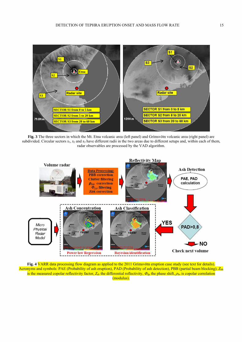
DETECTION OF TEPHRA ERUPTION ONSET AND MASS FLOW RATE
15
Fig. 3 The three sectors in which the Mt. Etna volcanic area (left panel) and Grímsvötn volcanic area (right panel) are
subdivided. Circular sectors s1, s2 and s3 have different radii in the two areas due to different setups and, within each of them,
radar observables are processed by the VAD algorithm.
Fig. 4 VARR data processing flow diagram as applied to the 2011 Grímsvötn eruption case study (see text for details).
Acronyms and symbols: PAE (Probability of ash eruption), PAD (Probability of ash detection), PBB (partial beam blocking). Zhh
is the measured copolar reflectivity factor, Zdr the differential reflectivity, dp the phase shift, hv is copolar correlation
(modulus).
Radar site S3
S2
S1
Etna
SECTOR S1 from 0 to 5 km
SECTOR S2 from 5 to 20 km
SECTOR S3 from 20 to 60 km
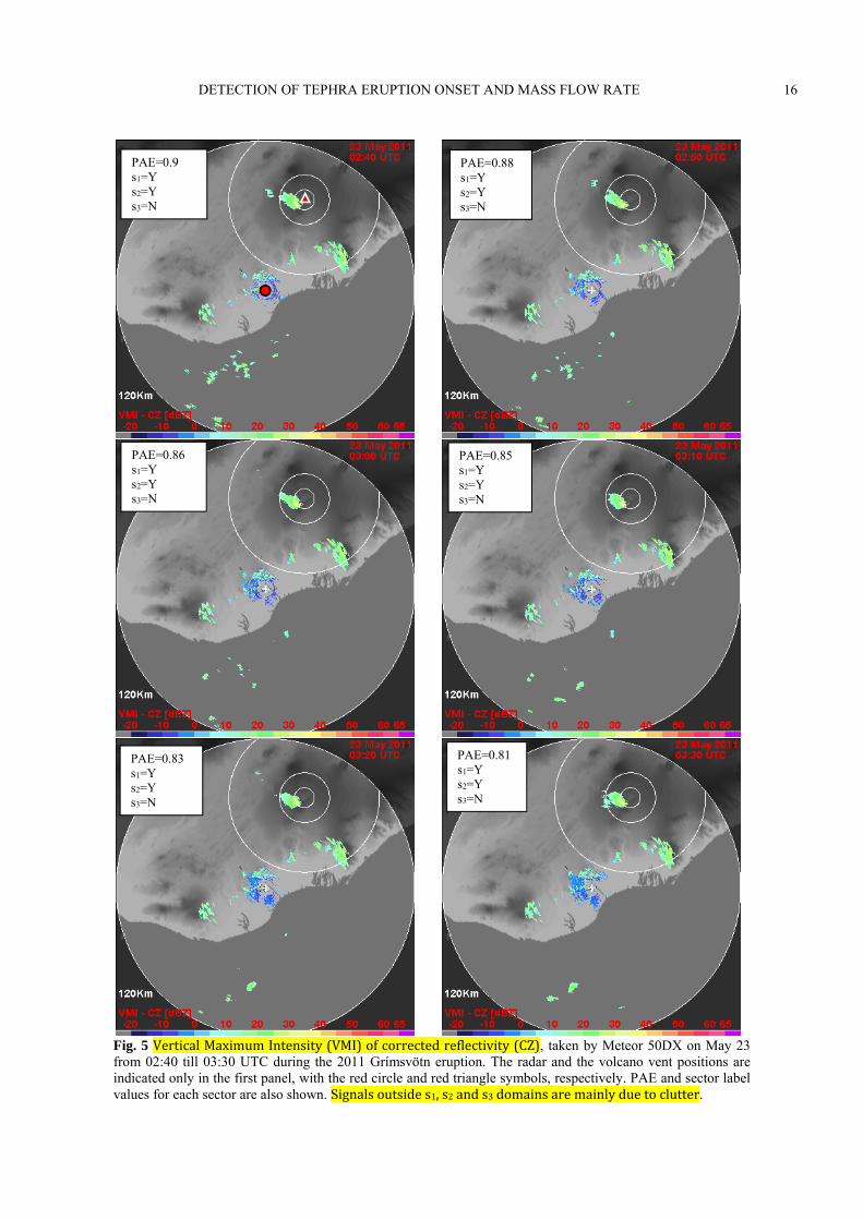
DETECTION OF TEPHRA ERUPTION ONSET AND MASS FLOW RATE
16
Fig. 5 VerticalMaximum)ntensity VM) ofcorrectedreflectivity CZ , taken by Meteor 50DX on May 23
from 02:40 till 03:30 UTC during the 2011 Grímsvötn eruption. The radar and the volcano vent positions are
indicated only in the first panel, with the red circle and red triangle symbols, respectively. PAE and sector label
values for each sector are also shown. Signalsoutsides ,s ands domainsaremainlyduetoclutter.
PAE=0.83
s1=Y
s2=Y
s3=N
PAE=0.81
s1=Y
s2=Y
s3=N
PAE=0.86
s1=Y
s2=Y
s3=N
PAE=0.85
s1=Y
s2=Y
s3=N
PAE=0.9
s1=Y
s2=Y
s3=N
PAE=0.88
s1=Y
s2=Y
s3=N

DETECTION OF TEPHRA ERUPTION ONSET AND MASS FLOW RATE
17
Fig. 6 Corrected VMI reflectivity images taken by Meteor 50DX on May 23 from 12:11 till 12:54 UTC during
the 2011 Grímsvötn eruption. The radar and the volcano vent positions are indicated only in the first panel, with
the red circle and red triangle symbols, respectively. PAE and sector label values for each sector are also shown.
PAE=1
s1=Y
s2=N
s3=N
PAE=0,9
s1=Y
s2=Y
s3=N
PAE=0,88
s1=Y
s2=Y
s3=N
PAE=0
s1=N
s2=Y
s3=N
PAE=0
s1=N
s2=N
s3=N
PAE=0,91
s1=Y
s2=N
s3=N

DETECTION OF TEPHRA ERUPTION ONSET AND MASS FLOW RATE
18
Fig. 7 Temporal sequence (sampled every 10 minutes) of PAE, extracted by VAD from X-band radar images on May 24-25,
2011 during the Grímsvötn eruption. Grey areas mark instants where a posteriori visual inspection confirmed the presence of the
plume at the Grímsvötn volcano.
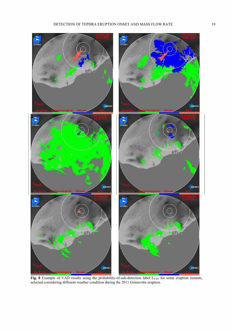
DETECTION OF TEPHRA ERUPTION ONSET AND MASS FLOW RATE
19
Fig. 8 Example of VAD results using the probability-of-ash-detection label LPAD for some eruption instants,
selected considering different weather condition during the 2011 Grímsvötn eruption.
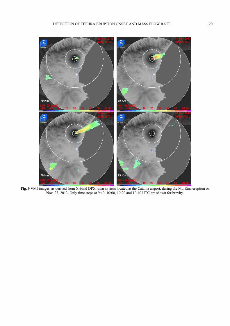
DETECTION OF TEPHRA ERUPTION ONSET AND MASS FLOW RATE
20
Fig. 9 VMI images, as derived from X-band DPX radar system located at the Catania airport, during the Mt. Etna eruption on
Nov. 23, 2013. Only time steps at 9:40, 10:00, 10:20 and 10:40 UTC are shown for brevity.

DETECTION OF TEPHRA ERUPTION ONSET AND MASS FLOW RATE
21
Fig. 10 Temporal sequence (blue curve) of estimated probability-of-ash-eruption (PAE), sampled every 10 minutes as extracted
by VAD from X-band radar data, on Nov. 23, 2013 during the Mt. Etna eruption. Grey areas mark instants where PAE was
labelled “Ash” and visual inspections confirmed the presence of an ash plume. Instantaneous mean pressure from IS array (pink
curve), sampled every 5 s and temporally averaged with 5-minute window, is also shown.
Fig. 11. Same as in Fig. 10, but for the plume maximum height above-the-sea-level derived from VARR.
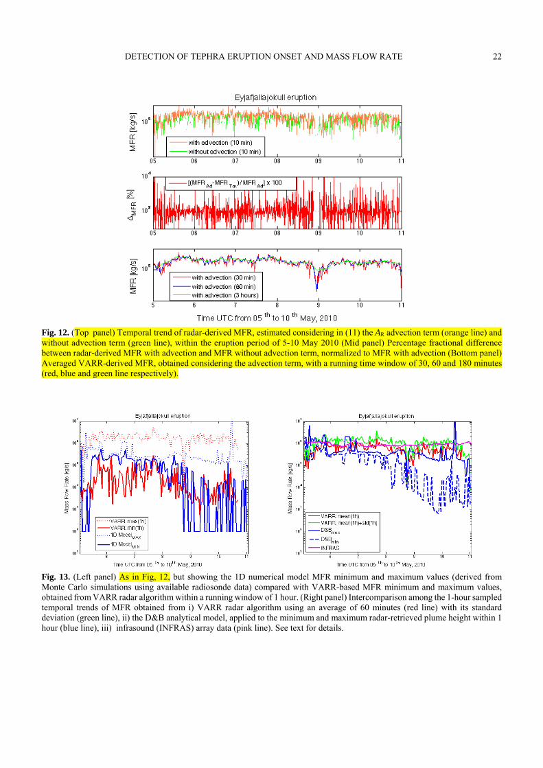
DETECTION OF TEPHRA ERUPTION ONSET AND MASS FLOW RATE
22
Fig. 12. (Top panel) Temporal trend of radar-derived MFR, estimated considering in (11) the AR advection term (orange line) and
without advection term (green line), within the eruption period of 5-10 May 2010 (Mid panel) Percentage fractional difference
between radar-derived MFR with advection and MFR without advection term, normalized to MFR with advection (Bottom panel)
Averaged VARR-derived MFR, obtained considering the advection term, with a running time window of 30, 60 and 180 minutes
(red, blue and green line respectively).
Fig. 13. (Left panel) As in Fig, 12, but showing the 1D numerical model MFR minimum and maximum values (derived from
Monte Carlo simulations using available radiosonde data) compared with VARR-based MFR minimum and maximum values,
obtained from VARR radar algorithm within a running window of 1 hour. (Right panel) Intercomparison among the 1-hour sampled
temporal trends of MFR obtained from i) VARR radar algorithm using an average of 60 minutes (red line) with its standard
deviation (green line), ii) the D&B analytical model, applied to the minimum and maximum radar-retrieved plume height within 1
hour (blue line), iii) infrasound (INFRAS) array data (pink line). See text for details.