Fragility of Mechanical, Electrical, and Plumbing · PDF fileFragility of Mechanical, Electrical, and Plumbing Equipment KeithPorter,a) M.EERI, GayleJohnson,b) M.EERI, RobertSheppard,c)

Fragility of Mechanical, Electrical, andPlumbing Equipment

Keith Porter,a)M.EERI, Gayle Johnson,b)

M.EERI, Robert Sheppard,c) andRobert Bachman,d)

M.EERI

A study for the Multidisciplinary Center for Earthquake EngineeringResearch (MCEER) provides fragility functions for 52 varieties of mechanical,electrical, and plumbing (MEP) equipment commonly found in commercialand industrial buildings. For the majority of equipment categories, theMCEER study provides multiple fragility functions, reflecting importanteffects of bracing, anchorage, interaction, etc. The fragility functions expressthe probability that the component would be rendered inoperative as a functionof floor acceleration. That work did not include the evidence underlying thefragility functions. As part of the ATC-58 effort to bring second-generationperformance-based earthquake engineering to professional practice, we havecompiled the original MCEER specimen-level performance data into apublicly accessible database and validate many of the original fragilityfunctions. In some cases, new fragility functions derived by ATC-58 methodsshow somewhat closer agreement with the raw data. Average-conditionfragility functions are developed here; we will address in subsequent work theeffect of potentially important—arguably crucial—performance-modifyingfactors such as poor anchorage and interaction. �DOI: 10.1193/1.3363847�

INTRODUCTION

In a project funded by the Federal Emergency Management Agency, the AppliedTechnology Council (ATC) is in the process of adapting for professional practice asecond-generation performance-based earthquake engineering (PBEE-2) methodologyoriginally developed by the Pacific Earthquake Engineering Research (PEER) Centerand others (e.g., Porter 2003). The methodology seeks to estimate the future seismic per-formance of buildings in terms of probabilistic repair costs, human safety, and function-ality (i.e., dollars, deaths, and downtime). A principal objective of the methodology isthat each stage of the analysis be objective and documented, with the least practical re-liance on expert opinion.

One stage of the analysis—referred to here as the damage analysis—seeks to esti-mate the probabilistic damage state of every damageable component of significance inthe building. The damage analysis follows a series of nonlinear time-history structuralanalyses, which produce probabilistic estimates of various measures of structural re-

a) SPA Risk LLC, Denver CO 80207, [email protected]) Halcrow, Oakland CAc) Energo Engineering, Inc., Houston TXd)
Consulting Structural Engineer, Laguna Niguel CA
451Earthquake Spectra, Volume 26, No. 2, pages 451–472, May 2010; © 2010, Earthquake Engineering Research Institute

452 PORTER ET AL.

sponse, referred to here as demands. Demand parameters may include member forces,deformations (including relative displacements between stories), and accelerations, ateach story, column line, or node.

In the damage analysis, demands are input to component fragility functions, one ormore fragility functions for each damageable component in the building. These fragilityfunctions relate a demand parameter to the probabilistic damage state of a fairly nar-rowly defined class of component. The level of resolution of the component categorysystem is fairly high: the ATC-58 taxonomy (Porter 2005) adds a subcategory system tothe NISTIR 6389 (NIST 1999) proposed extension to the UNIFORMAT-II componentnumbering system. UNIFORMAT II (ASTM 2002) has 58 categories of building com-ponent and NISTIR 6389 has 284, but neither distinguishes important seismic featuressuch as battery racks with or without anchorage or battery spacers—features that can becrucial to making informed seismic risk-mitigation decisions, thus the additional level ofthe taxonomy to distinguish such features is important.

There are three important implications for using this level of detail: First, one canresolve the difference in seismic performance of a particular building built with andwithout common seismic deficiencies. Second, one can use laboratory evidence andpost-earthquake field observations to support the fragility functions with a degree of ob-jectivity or verifiability. But counterbalancing these two perceived advantages is a prob-lem: at this level of detail a lot of fragility functions are needed—probably hundreds—torepresent most of the damageable components in most U.S. buildings and properly in-form mitigation decisions. Many of these required fragility functions—perhaps one-third—are mechanical, electrical, and plumbing (MEP) equipment. Where are they tocome from? There are several alternatives: laboratory testing, earthquake experience,theory, or expert opinion, but each choice involves time and expense.

Johnson et al. (1999, henceforth referred to as J99, and written largely by two of thepresent authors) provide a large number of MEP fragility functions: 52 component cat-egories, each with between one and eight variants to reflect seismic conditions, for atotal of approximately 170 fragility functions. This is enough potentially to serve a largeportion of ATC-58’s ultimate need for equipment fragilities.

J99 uses primary source data (some of which were also compiled in the EPRI SQUGdatabase, e.g., EPRI 2003) to develop fragility functions for approximately 15 compo-nent categories of MEP equipment, listed in Table 3. Each category has between fourand eight fragility functions to reflect installation conditions, for a total of 93 fragilityfunctions. The data used to create fragility functions for these components come fromdirect observation of equipment exposed to strong motion shaking in 23 earthquakes be-tween 1971 (San Fernando) and 1993 (Guam), including 123 sites experiencing groundmotions from 0.12 g to 0.85 g of geometric-mean-direction peak ground acceleration. Thefragility functions were published, but the underlying data were not. We refer to this previ-ously unpublished data set as the J99 database. The remaining 80 or so fragility functions—e.g., for breakage of buried pipe and for tank ruptures—were drawn from other authoritiesand are not addressed here.

The challenge in using the J99 fragility functions for ATC-58 is that, under devel-

FRAGILITY OF MECHANICAL, ELECTRICAL, AND PLUMBING EQUIPMENT 453

oping ATC-58 guidelines, fragility functions carry little weight if the underlying data arenot publicly available for review and validation. We therefore present them here and re-analyze them using ATC-58 procedures as described in ATC’s developing Guidelines forSeismic Performance Assessment of Buildings. The specimen-by-specimen observationsare presented here for the first time.

SUMMARY OF JOHNSON ET AL. SUPPORTING DATA

A database was compiled from the original, unpublished data used to create the J99fragility functions. The data are available at www.risk-agora.org. The database containstwo tables: one showing equipment damage data (the table is named “Damage”), theother summarizing the distribution of equipment through the height of the buildings inwhich they were observed (table name “Height”).

A sample of the damage data is shown in Table 1. Each record of table “Damage”contains observations of a particular class of component at a single facility in a singleearthquake. The database also contains the estimated shaking intensity at the facility, thetotal number of specimens (“units”), the number that failed, and in some cases a com-ment on the nature of the damage.

A sample of the table “Height” is shown in Table 2. Each record refers to the distri-

Table 1. Sample of failure database

Component Earthquake Facility PGA Units Failed Comments

Air compressor San Fernando 1971 GlendalePower Plant

0.25 4

Air compressor Morgan Hill 1984 IBM/SantaTeresa Facility

0.37 3

Air compressor Loma Prieta 1989 Green GiantFoods

0.30 2 2 Burnt windings dueto power transientsor single phasing

(The table also contains an integer index field, not shown here)

Table 2. Sample of table “Height”

Component Earthquake Facility PGA UnitsBot1 /3

Mid1/3

Top1/3

Air compressor San Fernando 1971 GlendalePower Plant

0.25 4 4

Air compressor Morgan Hill 1984 IBM/SantaTeresa Facility

0.37 3 3

Air compressor Chile 1985 Rapel HydroelectricPlant

0.23 8 6 2

(The table also contains an integer index field, not shown here)

454 PORTER ET AL.

bution through the height of a facility of a given component category in a single earth-quake. It shows the component category, earthquake, facility name, estimated PGA, totalnumber of specimens observed, and the number of specimens in each of the bottom,middle, and top one-third of the height of the facility. These data are relevant becauseexcitation is only known in terms of peak ground acceleration (PGA) at the site.

The nature of the buildings in which these specimens were observed is not recordedin the J99 database: not their height, nor lateral force resisting system, nor fundamentalperiod of vibration. Except for components that were installed on the ground floor, onlya crude estimate is practical for the peak excitation to which their bases were subjected.While PGA is a reasonable proxy for the acceleration to which specimens at the groundlevel or perhaps in the lower one-third of a building were subjected, the actual accelera-tion that specimens in the middle and upper one-third of floors experienced is unknown;amplification is dealt with in an approximate way, described later. (Note that most of thecomponents in the J99 database were installed in the lower third, so PGA is not a badproxy for the equipment demand parameter.) Note that there is not a one-to-one corre-spondence of records in Table “Height” to records in table “Damage” because the data-base did not always contain information about height distribution.

Tables 3 and 4 summarize the data examined here. In the table, each row refers toone category of component. “NISTIR 6389” refers to the approximate NISTIR 6389UNIFORMAT-II label for that category. Note some overlap: batteries in racks and bat-tery chargers both belong to D5092, Emergency Light and Power Systems, but are dis-

Table 3. Summary of data supporting 15 categories of fragility functions in Johnson et al.(1999)

Component categoryNISTIR6389 Events Sites Specimens Failed

Heightdistr.

Derivedfunctions

Air compressors D3032? 14 37 158 3 98,0,2 6Air handling units D3063 11 23 119 21 10,70,20 7Batteries in racks D5092 10 23 168 14 75,8,16 7Battery chargers D5092 18 46 156 2 96,4,0 6Chillers D3031 6 16 50 12 100,0,0 6Control panels D3067? 17 61 326 23 70,16,13 6Distribution panels D5012? 15 34 199 3 100,0,0 5Engine generators D5092 13 36 157 13 100,0,0 7Fans D3041 16 41 402 47 23,3,74 8Low voltage switchgear D5012? 19 45 150 7 98,2,0 6Motor control centers D5010 19 51 283 5 69,25,6 6Motor generators D5012? 12 18 41 0 91,9,0 7Pumps D3040? 19 44 551 5 100,0,0 7Transformers D5011? 18 46 245 5 100,0,0 5Valves D3040? 17 42 914 6 68,17,15 4Total 3919 166 93


tinct components with distinct seismic installation and fragility features. The column la-beled “Events” indicates the number of earthquakes after which various specimens wereobserved. The column labeled “sites” indicates how many different facilities were ex-amined; “specimens” indicates how many unique specimens were examined, and“failed” indicates distinct failures of those specimens.

The column labeled “Height distribution” recaps the percentage of observed speci-mens that were in the lower, middle, and upper one-third of buildings. The column la-beled “Derived functions” indicates how many fragility functions were derived from theEPRI data. As will be shown later, one basic fragility function was developed for eachclass of component, along with three or more additional fragility functions to reflect dif-ferent installation conditions, referred to in J99 as performance modification factors, orPMFs. For example, 6 fragility functions are derived for air compressors: (1) basic con-ditions, (2) no anchorage, (3) poor anchorage, (4) vibration isolator concerns, (5) rigidattachments, and (6) interaction concerns.

Few records in the J99 data actually indicate the presence or absence of PMFs. Thefragility functions for PMFs were developed using a methodology referred to in J99 as“survival analysis,” which involves observations of damage to component where PMFinformation is available. The effect on fragility from some of these PMFs is profound,increasing the failure probability in some cases by an order of magnitude or more. Thisimplies that in many cases the equipment itself is fairly rugged, but that anchorage, in-teraction, and other installation conditions should be the focus of remedial action.

Table 4. Fragility functions derived from Johnson et al. (1999) data

Component hNew MCEER

Diff in �2 Comment� � � �

Air compressor 1.02 2.2 0.6 2.5 0.4 −0.01Air handling unit 1.55 1.4 0.6 1.9 0.5 −0.27Batteries in rack 1.21 3.0 0.6 2.5 0.4 −0.15Battery charger 1.02 4.2 0.6 2.0 0.4 −0.01Chiller 1.00 0.7 0.6 2.1 0.5 −0.12Control panel 1.21 2.3 0.4 2.3 0.4 −0.20Distribution panel 1.00 3.4 0.6 2.8 0.4 −0.00Engine generator 1.00 1.6 0.6 2.0 0.4 −0.01Fan 1.75 1.4 0.6 1.6 0.5 −0.44Low voltage switchgear 1.01 1.2 0.6 1.3 0.4 −0.30Motor control center 1.18 1.8 0.6 1.5 0.4 −0.10Motor generator 1.05 1.5 0.4 2.0 0.4 N/A No failures;

method C usedPump 1.00 2.6 0.6 3.0 0.4 −0.01Transformer 1.00 1.3 0.6 1.6 0.4 −0.72Valve 1.23 4.5 0.6 4.0 0.4 −0.00

456 PORTER ET AL.

The methodology is explained in J99, but it involves assuming the lowest observedPGA associated with failure is the HCLPF (high confidence of low probability of fail-ure) PGA, defined as the PGA where the authors have 95% confidence that no more than5% of samples of the component would fail. With the addition of two beta values, onecan find the median failure PGA from the HCLPF PGA; the authors used

� = rHCLPF exp�1.65��u + �r�� 1�

where �u reflects modeling uncertainty (uncertain median) and �r represents uncertaintygiven a known median.

Equation 1 is rational, but is not used here for two reasons: (1) it has not yet beenaccepted as an ATC-58 standard, and (2) some of the rHCLPF values are based on judg-ment. For example, rHCLPF for motor control centers with interaction concerns is noted in theJ99 authors’ calculations as 0.2 g, but no specimens were actually observed where interac-tion was noted as contributing to failure. For this reason, the present manuscript addressesonly average-condition fragility functions; PMFs will be dealt with in a separate work. It isvaluable to know how equipment will perform when one knows installation conditions, but itis also valuable to know something about performance under average conditions, where thedetails of installation are unknown. Hence the average-condition fragility functions are wor-thy of consideration.

DEVELOPING FRAGILITY FUNCTIONS FOR HVAC EQUIPMENT

Methodology for height modifiers. J99 estimated the average floor acceleration ofequipment by increasing PGA by a factor to account for building response. Let M denotethe total number of specimens of a component class, ML the total number in the bottomone-third of the facilities they are in, MM the total number in the middle one-third, andMH the total number in the top one-third. Let PGAi denote the estimated geometric-meanpeak ground acceleration of the facility in which specimen i was observed, and let ri denotethe estimated floor acceleration of the specimen. It is estimated as

h =1

M�ML + 1.5 · MM + 2MH�

ri = h · PGAi �2�

Method B for developing fragility functions. A methodology is proposed in Guide-lines for Seismic Performance Assessment of Buildings (also shown in Porter et al. 2007)to estimate the fragility function of a component category where the available data aregroups (or bins) of components assumed to have experienced the same demand, wherebins contain varying number of specimens, and where at least some specimens failed.One performs a weighted least-squares fit to failure-rate data, using the number of speci-mens in each bin as the bin weight. Let


M = number of specimens observedi = index of specimens, i� �1,2 , . . .M�ri = demand to which specimen i was subjectedfi = failure indicator for specimen i

= 1 if specimen i failed (reached or exceeded damage state dm)= 0 otherwise

N = number of binsj = index of bins, j� �1,2 , . . .N�Mj = number of specimens in bin jmj = number of failed specimens in bin jyj = failure rate in bin j

yj =mj

Mj�3�

One finds � and �r to minimize �2 such that:

�2 =1

M�j=1

M

Mj�yj − �� ln�rj/��r

2

� � 0

0.2 � �r � 0.6 �4�

then calculates �:

� = �r2 + �u

2 �5�

where �u=0.25 if any of the following is true, 0 otherwise:All specimens were observed to be in the same configuration (if applicable)All specimens were observed to have the same installation conditionsAll specimens experienced the same loading historyM�5

Method C for developing fragility functions. In cases were no specimens failed, theGuidelines propose the following procedure for creating fragility functions. Given nodamage among M observations, letFdm�r�= failure probability given demand rri = demand experienced by specimen i�i=1,2 , . . .M�rmax = maxi�ri�rd = minimum demand experienced by any specimen with distressra = the smaller of rd and 0.7·rmax

MA = number of specimens without apparent distress and with ri�ra

MB = number of specimens at any level of ri with distress not suggestive of imminentfailure

458 PORTER ET AL.

MC = number of specimens at any level of ri with distress suggestive of imminentfailure

rm = rmax if MB+MC=0= 0.5· �rmax+ra� otherwise

S = subjective failure probability at rm

S = �0.5MC + 0.1MB�/�MA + MB + MC� �6�

One uses Table 5 to determine Fdm�rm� and Equation 7 to determine � and �.

� = 0.4

z = �−1�Fdm�rm��

xm = rm exp�− z�� 7�

RESULTS

New fragility functions and comparison with original. The J99 data were analyzedto produce values of h for each component category; the results are shown in Table 4.They agree in every case with the height modifier calculated in J99. The table also showsresults of the fragility analysis described above. The columns labeled “new” are param-eters for the fragility function re-derived from the raw data. The columns labeled“MCEER” are the fragility function parameters from J99. The difference between thetwo fragility functions is measured here by the relative difference in �2 calculated usingthe two sets, i.e., if we denote by �0

2 and �12 respectively the values of �2 as calculated

using the MCEER parameters and using the new parameters, then the difference noted inthe table is calculated by

Diff =�0

2 − �12

�12 �8�

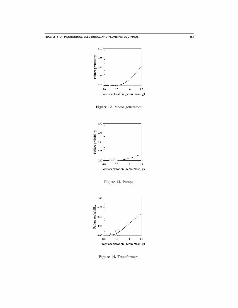
In only a few cases are there significant differences between the perceived accuracyof the newly derived versus original J99 fragility functions. Most notable among theseare the fragility functions for transformers and for fans, with 72% lower and 44% lower�2 values (equal to the reduction in residual variance). These differences are attributable

Table 5. Example values of exp�−z��

Conditions Fdm�rm� Zexp�−z��,

�=0.4

MA�3 and S=0 0.01 −2.326 2.54MA�3 and S�0.075 0.05 −1.645 1.930.075�S�0.15 0.10 −1.282 1.670.15�S�0.3 0.20 −0.842 1.40S�0.3 0.40 −0.253 1.11


to the fact that the authors of J99 constrained their � values to 0.4 or 0.5. The �=0.5value is reserved for components where a majority of the observed specimens were in themiddle and upper one-third of the building. In this work we have allowed � to vary between0.2 and 0.6 regardless of height. This greater latitude allows for a closer fit to the data.

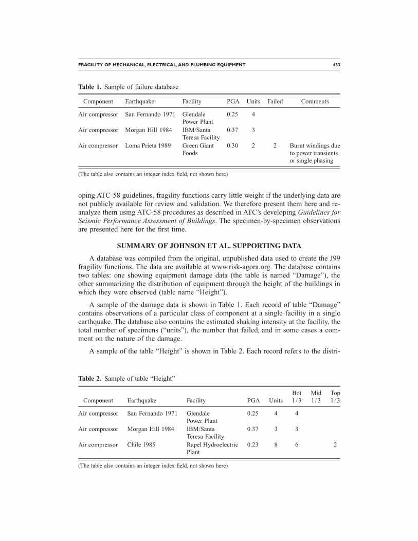
Figure 1 through Figure 15 show the derived fragility functions and the underlyingdata points, one point for each level of intensity (which can reflect one or more facili-ties). In the figures, “floor acceleration” means the geometric-mean peak horizontal ac-celeration applied at the base of the equipment, i.e., the floor slab on which the equip-ment stood. The figures all show a smooth curve for a fragility function between 0 and1.5 g, but with a dashed line above 1.5 times the maximum acceleration any of the speci-mens experienced. To use the curve extrapolated beyond that point is probably inappro-priate. Table 6 through Table 20 contain summary exposure and damage data for the

Figure 1. Air compressors.

Figure 2. Air handling units.

460 PORTER ET AL.

Figure 3. Batteries in racks.

Figure 4. Battery chargers.

Figure 5. Chillers.


Figure 6. Control panels.

Figure 7. Distribution panels.

Figure 8. Engine generators.

462 PORTER ET AL.

Figure 9. Fans.

Figure 10. Low voltage switchgear.

Figure 11. Motor control centers.


Figure 12. Motor generators.

Figure 13. Pumps.

Figure 14. Transformers.

Figure 15. Valves.

464 PORTER ET AL.

Table 6. Failure data of air compressors

r, g Units, M Failed, m w=M /M y=m /M �

0.20 16 0 0.101 0.000 0.0000.23 8 0 0.051 0.000 0.0000.24 4 0 0.025 0.000 0.0000.25 25 0 0.158 0.000 0.0000.26 11 0 0.070 0.000 0.0000.31 44 2 0.278 0.045 0.0000.33 3 0 0.019 0.000 0.0010.36 4 0 0.025 0.000 0.0010.38 3 0 0.019 0.000 0.0020.41 11 1 0.070 0.091 0.0020.43 7 0 0.044 0.000 0.0030.51 8 0 0.051 0.000 0.0070.57 2 0 0.013 0.000 0.0120.61 10 0 0.063 0.000 0.0160.65 2 0 0.013 0.000 0.021


Table 7. Failure data of air handling units


0.31 3 1 0.025 0.333 0.0000.39 7 0 0.059 0.000 0.0010.40 2 0 0.017 0.000 0.0010.46 2 0 0.017 0.000 0.0020.54 3 1 0.025 0.333 0.0060.57 3 0 0.025 0.000 0.0080.62 30 12 0.252 0.400 0.0130.65 6 2 0.050 0.333 0.0160.77 54 5 0.454 0.093 0.0360.87 2 0 0.017 0.000 0.0580.93 6 0 0.050 0.000 0.0761.32 1 0 0.008 0.000 0.232

Table 8. Batteries in racks failure data


0.17 5 0 0.030 0.000 0.0000.24 18 0 0.107 0.000 0.0000.28 5 0 0.030 0.000 0.0000.29 6 0 0.036 0.000 0.0000.30 41 6 0.244 0.146 0.0000.31 10 0 0.060 0.000 0.0000.36 24 2 0.143 0.083 0.0000.39 1 0 0.006 0.000 0.0000.42 10 3 0.060 0.300 0.0000.48 17 1 0.101 0.059 0.0000.51 2 0 0.012 0.000 0.0000.57 2 0 0.012 0.000 0.0000.60 14 1 0.083 0.071 0.0000.68 4 0 0.024 0.000 0.0010.72 6 1 0.036 0.167 0.0010.78 1 0 0.006 0.000 0.0021.02 2 0 0.012 0.000 0.013

466 PORTER ET AL.

Table 9. Failure data for battery chargers

r, g Units. M Failed, m w=M /M y=m /M �

0.14 4 0 0.026 0.000 0.0000.20 18 0 0.115 0.000 0.0000.23 10 0 0.064 0.000 0.0000.24 6 0 0.038 0.000 0.0000.25 27 0 0.173 0.000 0.0000.26 4 0 0.026 0.000 0.0000.31 21 0 0.135 0.000 0.0000.33 3 0 0.019 0.000 0.0000.36 12 1 0.077 0.083 0.0000.41 19 1 0.122 0.053 0.0000.43 4 0 0.026 0.000 0.0000.48 2 0 0.013 0.000 0.0000.51 10 0 0.064 0.000 0.0000.57 5 0 0.032 0.000 0.0000.61 7 0 0.045 0.000 0.0000.66 1 0 0.006 0.000 0.0000.87 3 0 0.019 0.000 0.000

Table 10. Failure data for chillers


0.20 4 0 0.080 0.000 0.0000.25 9 8 0.180 0.889 0.0000.30 5 0 0.100 0.000 0.0000.35 6 0 0.120 0.000 0.0000.37 4 0 0.080 0.000 0.0000.40 12 2 0.240 0.167 0.0000.42 6 2 0.120 0.333 0.0010.50 2 0 0.040 0.000 0.0020.60 2 0 0.040 0.000 0.006


Table 11. Failure data for control panels


0.17 6 0 0.018 0.000 0.0000.18 3 0 0.009 0.000 0.0000.24 17 1 0.052 0.059 0.0000.28 11 1 0.034 0.091 0.0000.29 10 0 0.031 0.000 0.0000.30 61 6 0.187 0.098 0.0000.31 18 0 0.055 0.000 0.0000.36 38 1 0.117 0.026 0.0000.39 10 0 0.031 0.000 0.0000.42 16 0 0.049 0.000 0.0000.45 1 0 0.003 0.000 0.0000.48 65 6 0.199 0.092 0.0000.51 8 0 0.025 0.000 0.0000.57 2 0 0.006 0.000 0.0000.60 32 4 0.098 0.125 0.0000.66 1 1 0.003 1.000 0.0010.68 8 0 0.025 0.000 0.0010.70 1 0 0.003 0.000 0.0010.73 5 2 0.015 0.400 0.0020.77 1 1 0.003 1.000 0.0030.79 3 0 0.009 0.000 0.0041.03 9 0 0.028 0.000 0.022

Table 12. Failure data for distribution panels


0.20 17 1 0.085 0.059 0.0000.24 19 0 0.095 0.000 0.0000.25 39 0 0.196 0.000 0.0000.26 10 0 0.050 0.000 0.0000.30 31 0 0.156 0.000 0.0000.35 7 0 0.035 0.000 0.0000.37 1 0 0.005 0.000 0.0000.40 33 2 0.166 0.061 0.0000.42 14 0 0.070 0.000 0.0000.50 12 0 0.060 0.000 0.0010.56 5 0 0.025 0.000 0.0010.60 5 0 0.025 0.000 0.0020.65 2 0 0.010 0.000 0.0030.85 4 0 0.020 0.000 0.011

468 PORTER ET AL.

Table 13. Failure data for engine generators


0.12 1 1 0.006 1.000 0.0000.14 1 0 0.006 0.000 0.0000.20 24 0 0.153 0.000 0.0000.23 4 0 0.025 0.000 0.0000.25 47 4 0.299 0.085 0.0000.26 1 0 0.006 0.000 0.0000.30 21 5 0.134 0.238 0.0000.35 5 0 0.032 0.000 0.0000.37 3 0 0.019 0.000 0.0000.40 18 1 0.115 0.056 0.0000.42 6 2 0.038 0.333 0.0000.50 5 0 0.032 0.000 0.0000.55 1 0 0.006 0.000 0.0010.56 1 0 0.006 0.000 0.0010.60 18 0 0.115 0.000 0.0010.85 1 0 0.006 0.000 0.016

Table 14. Failure data for fans


0.35 58 8 0.144 0.138 0.0000.42 5 0 0.012 0.000 0.0000.44 64 5 0.159 0.078 0.0000.46 26 0 0.065 0.000 0.0000.53 112 0 0.279 0.000 0.0000.56 4 0 0.010 0.000 0.0010.61 6 3 0.015 0.500 0.0020.65 2 0 0.005 0.000 0.0020.70 40 20 0.100 0.500 0.0040.74 30 4 0.075 0.133 0.0060.82 6 0 0.015 0.000 0.0130.88 21 4 0.052 0.190 0.0201.05 23 3 0.057 0.130 0.0541.12 5 0 0.012 0.000 0.074


Table 15. Failure data for low voltage switchgear


0.20 17 0 0.114 0.000 0.0020.23 6 0 0.040 0.000 0.0040.24 5 0 0.034 0.000 0.0050.25 38 3 0.255 0.079 0.0050.26 6 0 0.040 0.000 0.0070.30 26 0 0.174 0.000 0.0130.35 6 0 0.040 0.000 0.0240.37 2 0 0.013 0.000 0.0290.40 20 1 0.134 0.050 0.0390.42 9 1 0.060 0.111 0.0470.47 1 0 0.007 0.000 0.0680.50 5 0 0.034 0.000 0.0830.56 3 1 0.020 0.333 0.1100.57 3 0 0.020 0.000 0.1150.65 2 0 0.013 0.000 0.164

Table 16. Failure data for motor control centers


0.24 37 0 0.131 0.000 0.0000.27 5 0 0.018 0.000 0.0010.30 68 2 0.240 0.029 0.0010.31 6 0 0.021 0.000 0.0010.35 49 0 0.173 0.000 0.0030.38 9 0 0.032 0.000 0.0040.41 12 0 0.042 0.000 0.0060.44 3 0 0.011 0.000 0.0080.47 35 0 0.124 0.000 0.0120.50 11 0 0.039 0.000 0.0140.56 10 2 0.035 0.200 0.0230.59 19 1 0.067 0.053 0.0290.66 4 0 0.014 0.000 0.0440.71 15 0 0.053 0.000 0.056

470 PORTER ET AL.

components listed in Table 4. The field labeled “�” indicates the cumulative distributionfunction that minimizes the weighted squared error, �2. In the tables, “r” means the samething as “floor acceleration.”

CONCLUSIONS

Johnson et al. (1999) present in an appendix a potentially valuable set of fragilityfunctions for 15 categories of mechanical, electrical, and plumbing (MEP) equipment,based on damage observations of 3,919 pieces of equipment from 123 sites and 23earthquakes. The underlying data are presented here for the first time and are re-examined to develop fragility functions for use in ATC-58. The newly derived fragilityfunctions generally agree with the originals. In a few cases, significant reduction in re-

Table 17. Failure data for motor generators


0.21 4 0 0.098 0.000 0.0000.25 2 0 0.049 0.000 0.0000.26 11 0 0.268 0.000 0.0000.27 3 0 0.073 0.000 0.0000.31 6 0 0.146 0.000 0.0000.42 3 0 0.073 0.000 0.0000.44 1 0 0.024 0.000 0.0000.49 6 0 0.146 0.000 0.0000.52 3 0 0.073 0.000 0.0000.59 2 0 0.049 0.000 0.000

Table 18. Failure data for pumps


0.20 81 0 0.147 0.000 0.0000.24 18 0 0.033 0.000 0.0000.25 96 3 0.174 0.031 0.0000.26 24 0 0.044 0.000 0.0000.30 116 0 0.211 0.000 0.0000.32 13 0 0.024 0.000 0.0000.35 18 0 0.033 0.000 0.0000.37 14 0 0.025 0.000 0.0010.40 54 2 0.098 0.037 0.0010.42 39 0 0.071 0.000 0.0010.47 14 0 0.025 0.000 0.0020.50 22 0 0.040 0.000 0.0030.56 2 0 0.004 0.000 0.0050.60 40 0 0.073 0.000 0.007


sidual uncertainty was achieved by relaxing restrictions on the logarithmic standard de-viation of capacity (the so-called dispersion parameter). The next step is to refine thesefragilities based upon differences in installation and other conditions called performancemodification factors (PMFs), which in many cases may be key to understanding andmitigation of equipment failure risk.

Table 19. Failure data for transformers


0.20 22 0 0.090 0.000 0.0010.23 1 0 0.004 0.000 0.0020.24 7 0 0.029 0.000 0.0020.25 57 2 0.233 0.035 0.0020.26 12 0 0.049 0.000 0.0030.30 42 0 0.171 0.000 0.0060.35 3 0 0.012 0.000 0.0120.37 4 0 0.016 0.000 0.0160.40 57 1 0.233 0.018 0.0210.42 14 0 0.057 0.000 0.0260.47 9 1 0.037 0.111 0.0390.50 6 0 0.024 0.000 0.0490.56 2 0 0.008 0.000 0.0710.60 7 1 0.029 0.143 0.0880.64 2 0 0.008 0.000 0.107

Table 20. Failure data for valves


0.25 175 0 0.191 0.000 0.0000.30 33 0 0.036 0.000 0.0000.31 157 3 0.172 0.019 0.0000.32 44 1 0.048 0.023 0.0000.37 129 1 0.141 0.008 0.0000.40 52 0 0.057 0.000 0.0000.43 31 0 0.034 0.000 0.0000.46 9 0 0.010 0.000 0.0000.49 72 0 0.079 0.000 0.0000.52 44 1 0.048 0.023 0.0000.58 14 0 0.015 0.000 0.0000.62 19 0 0.021 0.000 0.0000.68 5 0 0.005 0.000 0.0000.69 9 0 0.010 0.000 0.0000.74 121 0 0.132 0.000 0.000

472 PORTER ET AL.

ACKNOWLEDGMENTS

The Applied Technology Council funded this work under a grant from the Depart-ment of Homeland Security to support ATC-58, Guidelines for Seismic Performance As-sessment of Buildings. Thanks to ATC-58 colleague Phil Schneider for his direction andassistance.

REFERENCES

American Society for Testing and Materials (ASTM), 2002. E1557-02 Standard Classificationfor Building Elements and Related Sitework—UNIFORMAT II, West Conshohocken, PA, 24pp.

Electric Power Research Institute (EPRI), 2003. SQUG Electronic Database User’s Guide, eS-QUG, Version 2.0 (QA)—Revision to TR-113705, Palo Alto, CA, http://www.epriweb.com/public/RS_1009040.pdf (viewed 1 May 2008).

Johnson, G. S., Sheppard, R. E., Quilici, M. D., Eder, S. J., and Scawthorn, C. R., 1999. SeismicReliability Assessment of Critical Facilities: A Handbook, Supporting Documentation, andModel Code Provisions, MCEER-99-0008, Multidisciplinary Center for Earthquake Engi-neering Research, Buffalo, NY, 384 pp.

National Institute of Standards and Technology (NIST), 1999. UNIFORMAT II Elemental Clas-sification for Building Specifications, Cost Estimating, and Cost Analysis, NISTIR 6389,Washington, D.C., 93 pp., http://www.bfrl.nist.gov/oae/publications/nistirs/6389.pdf (viewed3 March 2006).

Porter, K. A., 2003. An overview of PEER’s performance-based earthquake engineering meth-odology, Proc. Ninth International Conference on Applications of Statistics and Probabilityin Civil Engineering (ICASP9), July 6–9, 2003, San Francisco, CA, Civil Engineering Riskand Reliability Association (CERRA), 973–980, http://spot.colorado.edu/~porterka.

Porter, K. A., 2005. A Taxonomy of Building Components for Performance-Based EarthquakeEngineering, PEER Report No 2005/03, Pacific Earthquake Engineering Research (PEER)Center, Berkeley, CA, 58 pp, http://www.sparisk.com/pubs/Porter-2005-Taxonomy.pdf.

Porter, K. A., Kennedy, R. P., and Bachman, R. E., 2007. Creating fragility functions forperformance-based earthquake engineering, Earthquake Spectra 23, 471–489.

(Received 4 May 2008; accepted 20 August 2009�

Documents

Fragility of Mechanical, Electrical, and Plumbing · PDF fileFragility of Mechanical, Electrical, and Plumbing Equipment KeithPorter,a) M.EERI, GayleJohnson,b) M.EERI, RobertSheppard,c)