Embed Size (px)
Citation preview
University of Southern Queensland
Faculty of Engineering and Surveying
Fracture Analysis of Vinyl Ester Composites
Cured under Microwave Conditions
A dissertation submitted by
CHAN, Wooi Lieh
In fulfillment of the requirements of
Course ENG 4111 and ENG 4112 Research Project
Towards the degree of
Bachelor of Engineering (Mechanical)
Submitted: November, 2006

Abstract
i
Abstract
The use of composites plays an important role in the fields of Mechanical and Civil
Engineering. The idea of using composite materials in the two afore mentioned fields
are no longer new. In the Fibre Composite Design and Development (FCDD),
University of Southern Queensland (USQ) many researches and experiments on new
lightweight materials and structures have been carried out. In the research, FCDD
found that the composites made from vinyl ester resins suffer considerable shrinkage
during hardening. With this issue in mind, research on the methods to decrease the
shrinkage of the composites had been carried out. Ku (2002) claimed that by having
vinyl ester composites cured under microwave conditions, such shrinkage can be
reduced. The material used was thirty three percent by weight flyash particulate
reinforced vinyl ester composite VE/FLYASH (33%). The purpose of this project is
to research, measure and compare the fracture toughness of vinyl ester composite
cured under ambient and microwave conditions by using the short bar test.
The specimens will then fractured by using the MTS 810 Material Testing Systems
and the value of fracture toughness was obtained through some calculations.
And finally the results will analyzed by using Latin Square, determine which
treatments were most effective in maintaining the fracture toughness while reducing
the shrinkage of vinyl ester composite, and by how much, and which are worthless, so
we can weight the economic alternatives.

Declaration
ii
Declaration

Certification
iii
Certification
I certify that the ideas, designs and experimental work, results, analyses and
conclusions set out un this dissertation are entirely my own effort, except where
otherwise indicated and acknowledged.
I further certify that the work is original and has been previously submitted for
assessment in any other course or institution, except where specifically stated.
CHAN, Wooi Lieh
Student Number: 0050027434
Signature
Date

Acknowledgments
iv
Acknowledgments
To my parents who are currently in Malaysia for their supports to give me a chance
have the opportunity and privilege to study in Australia to attain my degree. This
would not be possible without them.
To Dr Harry Ku, for spending his valuable time in giving me ideas, guidance and
consultation, also his expertise in the experimental works as well as editing this thesis;
And also guiding me in doing this whole project from the starts. Thank you for your
advice, teaching, guidance and expertise.
To Mohan Trada for for assisting in setting up the equipment and providing
information and his patience and time in providing me the accessories and tools that
are required to carry out my project.
CHAN, Wooi Lieh
University of Southern Queensland
November 2006
Contents
v
Contents
Abstract..........................................................................................................................i
Declaration....................................................................................................................ii
Certification.................................................................................................................iii
Acknowledgments.......................................................................................................iv
List of Figures...............................................................................................................x
List of Tables...............................................................................................................xi
Chapter 1 Introduction���������������������.........1
1.1 Project aim������������������........����.1
1.1.1 Specific Objectives �����������........����.1
1.2 Dissertation Overview�������������........����...2
Chapter 2 Composite Material��������������........����.5
2.1 Introduction������������������........���...5
2.2 Type of Composite Material������������........���.6
2.3 Composite Benefits��������������........����..9

Contents
vi
2.4 The Basics of Polymers������������........����...12
2.5 Thermoset versus Thermoplastic��������...........����.13
2.6 Thermosetting Resins�����������������...�...14
2.7 Polyester Resins......................................................................................16
2.8 Specialty Polyesters................................................................................16
2.9 Epoxy Resin............................................................................................17
2.10 Thermoplastic Resins..............................................................................18
2.11 Vinyl Ester...............................................................................................19
2.11.1 History and commercial of Vinyl Ester.....................................19
Chapter 3 Their Interactions of Resins with Microwaves...................................21
3.1 Introduction.............................................................................................21
3.2 Vinyl Ester Resins...................................................................................22
3.3 Cross-linking of Vinyl Esters..................................................................23

Contents
vii
3.4 Shrinkage in VE/Fly-ash (33%)..............................................................27
3.5 Fundamentals of Microwaves.................................................................33
3.6 Microwave and material interactions�������������...34
Chapter 4 Fracture Mechanics...............................................................................37
4.1 Description of Fracture Mechanics..........................................................37
4.2 Fracture Toughness..................................................................................37
4.3 The Role of Fracture Mechanics.............................................................40
4.4 Theories of Mechanics and Fracture Toughness.....................................41
4.5 Transition Temperature Approach...........................................................44
4.6 Linear Elastic Fracture Mechanics...........................................................48

Contents
viii
4.7 Stress Intensity Factor..............................................................................49
Chapter 5 Test of Fracture Toughness..................................................................53
5.1 Description of Fracture Toughness Tests.................................................53
5.2 Standard Test Methods.............................................................................54
5.2.1 Compact Tensile Specimen............................................................54
5.2.2 C-Shape Specimen.........................................................................55
5.3 Non-Standard Test Methods.....................................................................56
5.3.1 Charpy V-Notch Test.....................................................................56
5.3.2 Short Bar Test.................................................................................57
5.4 Analysis of Fracture.................................................................................59
5.4.1 Brittle Fracture...............................................................................60
5.4.2 Ductile Fracture..............................................................................61
Chapter 6 Short Bar test.........................................................................................62
6.1 Standard Tests..........................................................................................62
6.2 Non Standard Tests..................................................................................63

Contents
ix
6.2.1 Short Bar Test.................................................................................63
6.3 Selection of the Short Rod or Bar Geometry...........................................75
6.4 Geometry of Specimen.............................................................................66
6.5 Short Bar Test Description.......................................................................69
Chapter 7 Experiment Method..............................................................................72
7.1 Specimen Preparation..............................................................................72
7.2 The Process of build up the Mould.........................................................72
7.3 Materials Preparation Progress................................................................77
7.4 Safety Measures......................................................................................78
7.5 Microwave Exposure of Composites......................................................79
7.5.1 The Modified Microwave Oven................................................79
7.5.2 Type of the Microwave Exposure Time....................................80

Contents
x
Chapter 8 Test Rig and Apparatus........................................................................81
8.1 Test Rig Requirements............................................................................81
8.2 Test Rig Available...................................................................................81
8.3 MTS 810 Material Testing Systems.........................................................82
8.4 The Advantages of MTS 810 Material Testing Systems.........................84
8.5 Gripper Design.........................................................................................85
Chapter 9 Results and Discussions........................................................................88
9.1 Introduction���������������������..........88
9.2 MTS-810 tensile testing machine�������������.........88
9.3 Fracture Toughness Determinations and Discussion�����...........93
9.3.1 The formulas and methods for calculating the fracture�..............94
toughness
9.3.2 Summary Results of Specimens����������.............96

Contents
xi
Chapter 10 Conclusion and Recommendations....................................................107
10.1 Conclusion............................................................................................107
10.2 Recommendations................................................................................108
List of Figures:
Figure 2.1: The classification of composites. ..................................................................................6
Figure 2.2: The properties of fiber composites.................................................................................7
Figure 2.3: Composite Benefits.........................................................................................................9
Figure 2.4: Particle-reinforced of elastics modulus........................................................................10
Figure 3.1: The structure of bishophenol A vinyl ester..................................................................23
Figure 3.2: Schematic of addition or free radical cross linking of vinyl ester. ..............................26
Figure 3.3: Temperature time relationships for cross linking of vinyl ester .................................27
Figure 3.4: Relationship between temperature and time in curing 200 ml of vinyl ester composite,
VE/FLYASH (33%) under ambient conditions. ...........................................................31
Figure 3.5: Relationship between temperature and time in curing 50 ml of vinyl ester composite,
VE/FLYASH (33%).......................................................................................................32
Figure 3.6: Degree of cure of vinyl ester at different curing temperatures ...................................32
Figure 3.7: Frequency Bands for Radio Frequency Range................................................................33
Figure 3.8: Interaction of Microwaves with Materials.......................................................................35
Figure 4.1: A specimen note that the entire crack length is equal to 2a. .......................................38
Figure 4.2: The general effect of temperature of the fracture resistance of structural metal ..........
........................................................................................................................................................45
Figure 4.3: Results from Charpy V-notch impact test. ..................................................................46
Figure 4.4: Fracture analysis diagram. ..........................................................................................57
Figure 4.5: The three basic modes of crack surface displacement (After Tada et al., 2000). ........50
Figure 4.6: Coordinate system for a crack tip................................................................................51
Figure 5.1: Compact tensile specimen. ...........................................................................................55
Contents
xii
Figure 5.2: The C-shape specimen. ................................................................................................55
Figure 5.3: Charpy V-notch test rig and sample............................................................................56
Figure 5.4: Short rod specimen configuration and dimensions. ....................................................58
Figure 5.5: The instruments magnification ranges ........................................................................59
Figure 6.1: Short bar specimens with curved chevron slots...........................................................66
Figure 6.2: Diagram of critical crack length ..................................................................................68
Figure 6.3: The equivalence for curved chevron slots....................................................................68
Figure 6.4: Variation of load versus crack length. .........................................................................70
Figure 7.1: The Auto-CAD drawing (a) and (b) for the triangle part of the mould. .....................73
Figure 7.2: The triangle mould for making the slot and important features of short bar specimen
.......................................................................................................................................74
Figure 7.3: The internal view of short bar specimen mould. .........................................................74
Figure 7.4: Explore view of mould. ................................................................................................75
Figure 7.5(a)&(b): Mould with canola oil. .....................................................................................76
Figure 7.6: The modified oven and its peripherals (Ku, H S 2002b) .............................................79
Figure 8.1: MTS 810 Material Testing Systems. .................................................................... ..�..82
Figure 8.2: Test rig with specimen in position ....................................................................... ..�..83
Figure 8.3: The systems of MTS 810 Material Testing Systems (MTS 810 FlexTest™
Material Testing Systems) ...................................................................................84
Figure 8.4: Grippers designs ..........................................................................................................86
Figure 8.5: The rounded profile of the grippers.............................................................................87
Figure 8.6: MTS 810 Material testing System................................................................................87
Figure 9.1: The fractured specimens and show the part for making the chevron slot ..................89
Figure 9.2: The change of load versus crack length of a sample cured under microwave condition
(720 Watt power level and 15-second exposure time). ..................................................91
Figure 9.3: Five critical points for the fractures surface to be analyzed........................................92
Figure 9.4: The change of load versus crack length of a sample cured under microwave condition
(720 Watt power level and 25-second exposure time). ..................................................92
Figure 9.5: Cross-section dimension of short bar specimen...........................................................93
Contents
xiii
Figure 9.6: Fracture toughness of VE/FLYASH (33%) cured under 180 Watts and 360 Watts of
microwave power. ....................................................................................................106
Figure 9.7: Fracture toughness of VE/FLYASH (33%) cured under 540 Watts and 720 Watts of
microwave power .....................................................................................................106
List of Tables
Table 2.1: Overview of properties exhibited different classes of material................................6
Table 3.1: Comparison of original and final volumes of VE/FLYASH (33%) .......................28
Table 3.2: Table 3.2: Frequency Bands for Radio Frequency Range.....................................34
Table 7.1: Weight of materials required to make 750ml of VE/FLYASH (33%)...................83
Table 7.2: Volume shrinkage and other parameters for 400 ml of VE/FLYASH (33%) exposed to
180-W microwaves at different duration ...............................................................87
Table 9.1: Test results of 720 Watts and 15-second exposure.................................................95
Table 9.2: Test results of ambient condition ...........................................................................96
Table 9.3: Test results of 180 Watts with 60 seconds ..............................................................97
Table 9.4: Test results of 180 Watts with 70 seconds ..............................................................97
Table 9.5: Test results of 180 Watts with 80 seconds ..............................................................98
Table 9.6: Test results of 360 Watts with 60 seconds ..............................................................98
Table 9.7: Test results of 360 Watts with 70 seconds. .............................................................99
Table 9.8: Test results of 360 Watts with 80 seconds ..............................................................99
Table 9.9: Test results of 540 Watts with 15 seconds ............................................................100
Table 9.10: Test results of 540 Watts with 20 seconds ..........................................................100
Table 9.11: Test results of 540 Watts with 25 seconds. .........................................................101
Table 9.12: Test results of 720 Watts with 15 seconds ..........................................................101
Table 9.13: Test results of 720 Watts with 20 seconds ..........................................................102
Table 9.14: Test results of 720 Watts with 25 seconds. .........................................................102
Table 9.15: Result of the fracture toughness and other parameters for VE/FLYASH (33%) cured
under different condition...................................................................................104

Contents
xiv
References.................................................................................................................110
Appendix A: Original Project Specification.................................................................a
Appendix B: Auto-CAD drawing.................................................................................d
Appendix C: Testing Results Obtained from MTS-810 of all
Conditions...............................................................................................g
Chapter 1 Introduction
1
Chapter 1
Introduction
1.1 Project aim
The aim of this project was about the analysis of fracture toughness on particulate
reinforced 33% Vinyl Ester composite cured under microwave conditions. The
shrinkage of the composites will be measured under ambient conditions and
microwave conditions.
1.1.1 Specific Objectives
This project will be produced specimens of 33 % VE/FLYASH under ambient
conditions and microwave conditions. These specimens are to investigate the fracture
toughness of 33% VE/FLYASH cured under ambient condition and microwave
conditions. During the curing process the vinyl ester suffers will occur shrinkage.
Therefore microwave energy in multimode oven cavity is to be applied to samples the
vinyl ester resins under controlled conditions to minimize its shrinkage.

Chapter 1 Introduction
2
1.2 Dissertation Overview
Here is the brief overview on the material presented on each chapter of the dissertation.
Chapter Two
Discuss on the background information of vinyl ester composites. This will be
followed by introducing to the reader a more detailed overview of the family of vinyl
ester material. The background overview on the materials used and produced will also
be introduced to the reader in the later part of this chapter.
Chapter Three
Discusses on the interaction between microwaves and materials used in this project.
The ways of microwaves can be used to reduce the shrinkage of the composite will
then be introduced to the reader. Various risks involved in curing using microwave
irradiation and the safety measures that needed to be undertaken will be discussed in
the later part of the chapter.
Chapter Four
Explain the fracture mechanics which defined as a field of solids mechanics that deal
with the behaviour of cracked bodies subjected to stresses and strains. The aims of the
fracture mechanics are to determine the severity of a pre-existing defect in term of its
tendency to initiate a fracture, which would cause failure.

Chapter 1 Introduction
3
Chapter Five
Introduce KIC (fracture toughness) which define as material of a sharp crack that has
the characteristics of its resistance to fracture under tensile conditions. It is extremely
important property in many crucial design applications.
Chapter Six
In-depth understanding of short bar test and the geometry of specimens. Compare the
disadvantages and advantages of both standard and non-standard testing.
Chapter Seven
Describe the preparation experimental work in this research project. Discussion on
production of specimens will be made first follow by preliminary testing on these
specimens. Discussion on data preparation and failure analysis will then be introduced
to reader.
Chapter Eight
Introduce the MTS 810 machine and the system which are use in the tensile testing of
this project.
Chapter Nine
The results obtained from the experimental work will be present in this chapter. The
chapter will be divided into sections; (1) related to e tensile testing results from the
experimental work, and (2) fracture toughness determination and discussions.

Chapter 1 Introduction
4
Conclusion
Conclusions and recommendations for this research project. This will include the
recommendations given by the author as a guide for further work in this project area.
Chapter 2 Composite Material
5
Chapter 2
Composite Material
2.1 Introduction
. In this project, particles will be dispersed in a polymer matrix. The background and
description of polymer matrix composites (PMCs) as well as their classification will
be introduced later. In the case of thermosets, the reader will be introduced to epoxies,
polyesters and vinyl ester.
A composite is a complex material, in which two or more distinct substances,
combine to produce functional and improved properties not present in any of the
individual component. This project relates to a polymer-based composite, which is
formed from the combination of fiber and resin, where the fibers are oriented to carry
the loads. Because of these aligned fibers that are meant to carry the loads and their
adaptive nature enabling the fibers to align in the direction to carry the load, these
composites can be designed to the minimum weight without sacrificing the strength.
Thus, generally, composites have stiffer, lighter and higher strength than the other
usual materials. In the case of this project, particles will be dispersed in a polymer
matrix. Introduction to the background, description and the classification of the
polymer matrix composites (PMCs) will be done later as well as the introduction of
epoxies, polyesters and vinyl ester in the case of thermosets.

Chapter 2 Composite Material
6
2.2 Types of Composite Materials
Either thermoset or thermoplastic, composites as a polymer matrix provides a
discernable reinforcing function in one or more directions when reinforced with a
fiber or other material with adequate aspect ratio (length to thickness). Bear in mind
that not all plastics are composites and that the majority of plastic materials available
today are pure plastics. This is in cases where products such as household goods, toys
and decorative products do not require very high strength for their functions and thus
plastic resin would be sufficient to provide the strength needed. Whereas for those
that are required to perform better, such as at increased heat distortion temperatures,
�engineering-grade� thermoplastics are of a better quality than the normal plastic
resins, but comes more costly. So, in fact, many types of plastics can be reinforced
with structural materials when additional strength is needed to fulfill the requirements
of higher performance. In most cases, reinforcing fibers are used. All these
thermoplastic or thermoset plastic resins that is reinforced with other material is then
considered a composite. Figure 2.1 shows the classification of composites.
Figure 2.1: The classification of composites
Chapter 2 Composite Material
7
Several types of composites are available especially for industrial use and most of
these composites are based on polymeric matrices, thermosets and thermoplastics.
Usually, aligned ceramic fibers, for example glass or carbon, are used to reinforce the
composites. Not long ago, interest in metal matrix composites (MMCs), such as
aluminium reinforced with ceramic particles or short fibers, and titanium containing
long, large-diameter fibers, has emerged. The property enhancements being sought by
the introduction of reinforcement are often less pronounced than for polymers, with
improvements in high-temperature performance or tribological properties. The
research and development area do come up with various industrial applications for
MMCs but in comparison to that of polymer composites (PMCs), MMCs are still
quite limited in terms of commercial usage. As for ceramic material composites
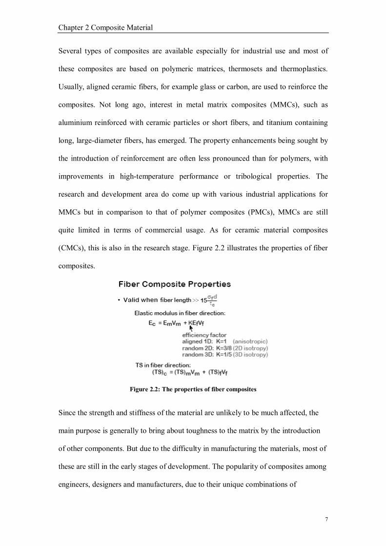
(CMCs), this is also in the research stage. Figure 2.2 illustrates the properties of fiber
composites.
Figure 2.2: The properties of fiber composites
Since the strength and stiffness of the material are unlikely to be much affected, the
main purpose is generally to bring about toughness to the matrix by the introduction
of other components. But due to the difficulty in manufacturing the materials, most of
these are still in the early stages of development. The popularity of composites among
engineers, designers and manufacturers, due to their unique combinations of

Chapter 2 Composite Material
8
performance benefits have caused the composites to arise, making jobs easier with
increased effectiveness for those associated in turning design concepts into product
realities.
It is crucial to look into the properties shown by the potential constituents when in
comes to considering formulating a composite material for particular applications.
The properties that are of particular interest are the stiffness (Young�s modulus),
toughness and strength of the material as well as density which is of great importance.
Apart from that, thermal properties, such as expansivity and conductivity, must also
be taken into account. Note that, because composite materials are subject to
temperature changes during manufacture and/or in service, an internal residual stress
would happen when there is a mismatch between the thermal expansivities of the
constituents and thus leading to a strong effect on the mechanical behavior. Some
representative property data are shown in the Table 2.1 for various types of matrix
and reinforcement, as well as for some typical engineering materials and a few
representative composites. Observing these data, it shows that some interesting
property combinations (e.g. high stiffness/strength and low density) can be obtained
through composites.

Chapter 2 Composite Material
9
Table 2.1: Overview of properties exhibited different classes of material
2.3 Composite Benefits
In any successful composites� application, there will usually be one or more of the
following benefits (Figure 2.3 shows the benefits of 3 types of composites):
Figure 2.3: Composite Benefits
1) High strength � Composites are materials most effective in delivering high
strength. Unlike the normal materials, it is able to have the strengths of
composites oriented or made to meet specific design requirements of an

Chapter 2 Composite Material
10
application. In general, composites are materials that could provide a wide
range of mechanical properties (tensile, flexural, impact compressive
strength).
2) Light weight � Comparing to the other plastics/metals which are not
reinforced, composites deliver more strength per unit of weigh and thus this
high strength/light weight combination is an additional benefit for the effective
use of composites.
3) Design Flexibility � A designer may want to form a material into any shape
and composites are flexible in this case to carry out this function, be it
complex or simple small or large structurally, for decorative or functional
purposes. With composites, many choices are available without having to
make costly trade-offs. Besides that, composites give the designers freedom to
try new approaches, from protoptype to production of the product. From the
Figure 2.4, it illustrates the particle-reinforced of elastics modulus.
Figure 2.4: Particle-reinforced of elastics modulus
4) Dimensional Stability � Thermoset composites are capable of maintaining
their shape and functionality under severe mechanical and environmental
stresses. Unlike the not reinforced thermoplastics, composites do not exhibit

Chapter 2 Composite Material
11
the viscoelastic or �cold-creep� characteristics. The coefficient of thermal
expansion is reduced. So, basically, the yield point of a composite is its break
point.
5) High Dielectric Strength � Another of composites� excellent properties is
electrical insulation, thus is a good choice for current carrying components.
Through the use of suitable modifiers and additives, imparting electrical
conductivity to composites is possible, which is required by the application.
6) Corrosion Resistance � Composites do not rust or corrode. For almost every
chemical and temperature environment, there are a couple of resin systems
which provide long-term resistance. Composite parts that are well designed
typically have long service life as well as minimum maintenance.
7) Parts Consolidation � Often, the assemblies of many parts and fasteners
required for normal materials, e.g. steel, are replaced by composite moldings.
By doing so, manufacturing costs can be reduced and parts are generally more
trouble-free.
8) Finishing � It is possible to mold colors into products in composite
applications for appearance that are durable yet with minimum maintenance.
Low profile and low-shrink resin systems are compatible with most metallic
painting operations. To reduce trim waste, flash, sanding and other
post-molding operations, proper design of molds and choice of materials are
essential.

Chapter 2 Composite Material
12
9) Low Tooling Cost � Tooling costs for materials such as steel, aluminum,
alloys, etc, are generally higher than the tooling costs for composites, in spite
of the processing methods selected.
10) Proven History of Successful Applications � In the last 45 years, there have
been over 50,000 successful composite applications that has have contributed
in proving the values of these materials. These days, engineers, designers
and marketing professionals can point with confidence to an expansion of end
uses and applications providing evidence of the cost and performance benefits
of composite unlike the days where the pioneers of the industry once struggled
to make this material accepted.
2.4 The Basics of Polymers
The term polymer comes from �poly� meaning many and �mer�, describing a unit.
Polymers are generally monomers, a single building block, that are joined together.
Composites usually are formed by polymers which come from sophisticated chemical
processing. A simple introduction to the basics of polymers would help to understand
the chemistry involved.
Basically, plastics are made up of the following significant chemical elements (in
shorthand notation):
C = Carbon
H = Hydrogen
O = Oxygen
An example of a typical polyester resin in shorthand:

Chapter 2 Composite Material
13
H � (OOC - C6H4 - COO - C2H4)n � OH
where the structure in the brackets repeats itself many times, as designated by the
number n. For a polymer, this would be a long chain and the value for n could be
greater than 100.
Thus, styrene would be shown as:
C6H5 � CH = CH2
2.5 Thermoset versus Thermoplastic
There are 2 major groups for resins or plastics: thermoset and thermoplastic. For
thermoplastic resins, when heated, they soften and thus enabling the process of
shaping or molding while in a heated semi-fluid state. As for thermoset resins, they
are usually in liquid state or are low-melting-point solids in their initial form. When
used to produce finished goods, these thermosetting resins are �cured� by using
catalyst, heat or both. Once the solid thermoset resins are cured, conversion back to
their original liquid form is no more possible. In other words, they will not melt and
flow when heated and cannot be reshaped.
Due to the dissimilar requirements of the fabrication process for thermosets and
thermoplastics, the composites industry has been divided into these two different
camps with both types still benefit from reinforcement. Initially, the growth of
composites was in thermosets; primarily glass fiber reinforced unsaturated polyester
resins. These days, the growth has moved to reinforced thermoplastics and is expected
to go on expanding due to the improved properties and effective cost of

Chapter 2 Composite Material
14
thermoplastics. Thus, it is crucial that those who consider using the composites have
sufficient knowledge about thermosetting and thermoplastic polymers.
2.6 Thermosetting Resins
The most common thermosetting resins used in the composites industry are
unsaturated polyester, epoxies, vinyl ester, polyurethanes and phenolics. In order to
select the proper material for a specific application, understanding of the difference
between these groups of resins is necessary.
2.7 Polyester Resins
Out of the total resins used, unsaturated polyester resins account for about 75% in the
composites industry. For injection molding of both composite and non-composite
parts, these resins are available in a different grade. Polyesters are produced by the
condensation polymerization of dicarboxylic acids and diayoric alcohols (glycols).
Apart from that, unsaturated materials, such as maleic anhydride or fumaric acid,
could be found in unsaturated polyesters as part of the dicarboxylic acid component.
The finished polymer is then dissolved in a reactive monomer, such as styrene, to give
a low viscosity liquid. The monomer reacts with the unsaturated sites on the polymer
once the resins are cured. Thus, this converts the polymer into a solid thermoset
structure.
Many different acids and glycols are used in polyester resins. The following lists some
of the common ones and the reasons as to why they are used:

Chapter 2 Composite Material
15
Due to the versatility of polyester, there are a range of raw materials and processing
techniques that are available in achieving the desired properties in the formulated or
processed polyester resins. Also, polyesters have been found to have almost absolute
usefulness in all segments of the composites industry due to their capacity to be
modified or tailored during the construction of the polymer chains. The principal
advantage of these resins is a balance of properties (mechanical, chemical and
electrical), dimensional stability, cost and ease of handling or processing.
Unsaturated polyesters are divided into classes depending on the structures of their
basic building blocks. For example, Orthophthalic (�ortho�), Isophthalic (�iso�),
Dicyclopentadiene (�DCPD�) and Bisphenol A. Fumarate resins. Besides that,
polyester resins are also classified according to the end use application as either a
general purpose (GP) or specialty polyester.

Chapter 2 Composite Material
16
2.8 Specialty Polyesters
A number of specialty polyesters are available. This is due to the capability of
polyesters in meeting the requirements of a range of applications when chemically
tailored. The specialty polyesters include:
• Flexibilized polyesters
• Electrical grade polyesters
• Corrosion-resistant polyesters
• Heat resistant polyesters
• Fire retardant polyesters
• Translucent polyesters
• Low shrink/low profile polyesters
The chemical makeup of a polymer brings about the performance of specialty
polyester. Properties such as fire resistance, fatigue performance and chemical
resistance could be enhanced with the correct use of fillers or additives. When one
property is improved, for example chemical resistance, other properties, such as
temperature resistance, may also be improved. An example is Bisphenol A Fumarate.
It has the ability to tolerate a range of chemical exposure and higher on-service
temperatures, thus is used for fabrication purposes.
Liquid styrenated polyester resins can be easily shipped to fabricators who do the
final shaping and curing of these materials into useful products. The reaction between
the unsaturation in the polyester and the styrene monomer is the mechanism for
curing resulting in the polyester chains being tied together by the styrene monomer.
Unlike epoxies and urethanes or phenolics, the curing of polyester resins differs in the

Chapter 2 Composite Material
17
sense than most epoxies and urethanes will begin to increase in viscosity the moment
they are catalyzed until they are cured. As for polyester, there is minor viscosity
increase or temperature change in a specific working time (gel time). Gelation takes
place when less than 5% of the original unsaturation has reacted and full cure occurs
very rapidly after this.
2.9 Epoxy Resin
Epoxy resin has a firm record where composite parts and structures are involved.
Many different products with a diversity of levels of performance can be produced
from engineered structure of epoxy resins. Also, they can be formulated with various
materials or blended with other epoxy resins to obtain a particular performance
characteristic. Hardeners and/or catalyst systems that are properly chosen enables cure
rates to be controlled to match process requirements. Epoxies are basically cures by
addition of an anhydride or an amine hardener and each of these hardener yields
different properties in the finished composite.
The primary uses of epoxies are generally in the fabrication of high performance
composites with superior mechanical properties, resistance to corrosive liquids and
environments, superior electrical properties, great performance at elevated
temperatures or any combination of these benefits. To provide a reasonable ground
for the superior performance but higher cost resin systems, critical applications on the
use of epoxies are usually required. An example of the use of epoxy resins are in the
marine automotive electrical appliance, besides other composite parts and structures.
However, provided that special performance is required, these are generally not cost

Chapter 2 Composite Material
18
effective in these markets. In comparison to most polyester resins, epoxy resins have
much higher viscosity and post-cure is required to achieve the ultimate mechanical
properties, thus are more difficult to use.
Besides being used with a number of fibrous reinforcing materials, including glass,
carbon and aramid, epoxy resins are also used as matrix resins for �whiskers� such as
boron, tungsten, steel, boron carbide, silicon carbide, graphite and quartz.
Nevertheless, the latter group is of small volume, comparatively high cost, and is
usually only used to achieve high strength and/or high stiffness requirements. Among
the benefits of epoxies are that they are readily usable with most composite
manufacturing processes. The processes in particular are pressure-bag molding,
vacuum-bag molding, compression molding, autoclave molding, hand lay-up and
filament winding.
2.10 Thermoplastic Resins
When combined with reinforcing fibers to produce a composite material,
thermoplastic resins provide unique and beneficial properties. Designers are drawing
advantages from the properties of the thermoplastic composite material in order to
improve the performance of the product as well as minimizing the manufacturing
costs. This differs from thermoset resins that are described as hard and somewhat
brittle. In other words, thermoplastic resins are characterized as tough and offers
superior impact resistance. Apart from that, the curing process for thermoplastic
resins to obtain their final properties also takes a shorter time, meaning, cycle times
are shorter, productivity is increased and the costs of parts are lower. What is of

Chapter 2 Composite Material
19
interest is that composites produced from thermoplastic resins especially in the
automotive markets, can be readily recycled, making it meet the demands of
environmental mandates. Besides, these resins are naturally impervious to attack from
harsh chemicals, petroleum products, environment products and environmental
elements. The group of thermoplastics resins is also large and wide-ranging, thus
enabling the selection of a resin based on specific properties tailored to the end
application.
2.11 Vinyl Ester
Vinyl ester was developed to merge the favorable qualities of epoxy resins with better
handling/ faster curing process typical for unsaturated polyester resins. By reacting
epoxy resins with acrylic or methacrylic acid, vinyl ester is produced providing an
unsaturated site. This is basically similar to that produced in polyester resins when
malefic anhydride is used. The material obtained it then dissolved in styrene, thus
producing a liquid much like the polyester resin. For the curing, this is done so on
vinyl esters with conventional organic peroxides (used with polyester resins).
In terms of mechanical toughness and corrosion resistance, vinyl ester shows these
beneficial qualities and these qualities are obtained with no complex processing,
handling or special shop fabricating practices involved unlike epoxy resins.
2.11.1 History and commercial of Vinyl Ester
Developed in the 1960s, vinyl ester resins are addition to the products of various
epoxy resins and unsaturated monocarboxylic. These are the most common materials

Chapter 2 Composite Material
20
to be mixed with acrylic acid. Combined with the best attributes of epoxies and
unsaturated polyesters, vinyl ester resins are easy to handle in room temperature. The
temperature and mechanical properties are alike to epoxies resins but generally have
better chemical resistance than cheaper polyester resins.
Chemical-wise, vinyl ester (VE) is related to unsaturated polyesters and epoxies, or
seems to be composed of these two. VE came about from an attempt in combining
the fast and simple cross linking of unsaturated polyesters with the mechanical and
thermal properties of epoxies.
This shrinkage is taken seriously especially when the components of the composites
are large that could go up to a value of more than 10%, much higher than claimed by
some researchers and resins� manufacturers (Clarke, 1996; Matthews, 1994). The
primary problem is due to the stresses set up internally. Usually, these stresses are
tensile in the core of the component and compressive on the surface (Osswald, 1995).
When the stresses act together with the applied loads during service, it causes a
premature failure in the components of the composites. The Fibre Composite Design
and Development (FCDD) group has solved this shrinkage problem by breaking the
large composite into smaller parts. The explanation to this was that the smaller
composite parts would have less shrinkage. These smaller parts would then be
combined into one to create the overall structure. All these are individual items of the
components that are produced by casting in liquid form, 44% uncured (by volume) or
33% (by weight). The vinyl ester is reinforced by flyash particulates in the moulds.
[VE/FLYASH (33%)].

Chapter 3 Interactions of Resins with Microwaves
21
Chapter 3
Interactions of Resins with Microwaves
3.1 Introduction
Unsaturated polyesters (UP), epoxies and vinyl esters were nowadays the most
widespread used as composite matrices in industry. Unsaturated polyesters dominate
the market, whereas epoxies are preferred in high-performance applications.
Unsaturated polyester offers an attractive combination of low price, reasonably good
properties, and simple processing. However, basic unsaturated polyester formulations
have drawbacks in terms of poor temperature and ultra-violet tolerance.
Additives may significantly reduce these advantages to suit most applications. Where
mechanical properties and temperature tolerance of unsaturated polyesters no longer
suffice, epoxies (EP) are often used due to their significant superiority in these
respects. Of course, these improved properties come at a higher price and epoxies
are used most commonly in areas where cost tolerance is highest (Astrom, 1997).
When epoxy resins are used to make composite structures, there are three main
drawbacks (Pritchard, 1999):
i) Because of their two-step hardening process, they are slow to cure, and
they require a minimum post cure of 2 to 4 hours at 120 oC to achieve
70-80% of optimal properties.
ii) Their viscosity makes it difficult to wet the glass fibres efficiently.

Chapter 3 Interactions of Resins with Microwaves
22
iii) The use of amine hardeners renders the cured resins susceptible to acid
attack.
With this issue in mind, the so-called epoxy vinyl ester range of resins (vinyl ester
resins) was developed in the 1960s (Pritchard, 1999). Vinyl esters (VE), as they are
usually called, are chemically closely related to both unsaturated polyesters and
epoxies and in most respects represent a compromise between the two. They were
developed in an attempt to combine the fast and simple cross linking of unsaturated
polyesters with the mechanical and thermal properties of epoxies (Astrom, 1997).
To achieve the project objectives, i.e. to reduce the shrinkage of vinyl esters, it will be
necessary to apply microwave energy in a multimode oven cavity to samples of vinyl
ester resins under controlled conditions. A commercial 1.8 kW microwave oven will
be used. The 1.8 kW power is actually achieved by launching microwaves from two
0.9 kW magnetrons. The power inputs can be varied from 10% (180 W) to 100%
(1800 W) in steps of 180 W.
3.2 Vinyl Ester Resins
Unsaturated resins such as polyesters and vinyl esters have ester groups in their
structures. Esters are susceptible to hydrolysis and this process is accelerated and
catalyzed by the presence of acids or bases. Vinyl esters contain substantially less
ester molecules than polyesters. They contain only one at each end of the resin
molecule. This is illustrated by the structure of bishophenol A vinyl ester in Figure
3.1. This means that vinyl esters, just like epoxies, have few possible crosslink sites

Chapter 3 Interactions of Resins with Microwaves
23
per molecule. Vinyl esters of high molecular weight will therefore have relatively
low crosslink density and thus lower modulus than if the starting point is a lower
molecular-weight polymer. Vinyl esters crosslink in time frames and under
conditions similar to those of unsaturated polyesters, i.e. fairly quickly and often at
room temperature (Astrom, 1997). Methacrylic acid is used to manufacture the vinyl
esters. This means that next to each ester linkage is a large methyl group. This
group occupies a lot of space and sterically hinders any molecule approaching the
ester group by impeding their access. These two aspects of the design of the
vinlyester molecule combine to make them more chemically resistant than polyesters
(Pritchard, 1999). There are three families of vinyl esters. The most commonly
used family is based on the reaction between methacrylic acid and diglycidylether of
bisphenol A (DGEBPA) as shown in Figure 3.1 (Astrom, 1997).
Figure 3.1: The structure of bishophenol A vinyl ester
3.3 Cross Linking of Vinyl Esters Resin
The polymerisation product between methacrylic acid and bisphenol A is vinyl ester,
which can be a highly viscous liquid at room temperature or a low melting point solid,
depending on the acid and bisphenol A used. For further processing, the polymer is
Chapter 3 Interactions of Resins with Microwaves
24
dissolved in a low molecular monomer, or reactive dilutent, usually styrene, the result
is a low viscosity liquid referred to as resin. The resin used in this research has 50%
by weight of styrene. With the addition of a small amount of initiator to the resin the
cross linking reaction, or curing, is initiated. The initiator used is organic peroxide,
e.g. methyl ethyl ketone peroxides (MEKP). The added amount is usually 1 to 2
percent by weight. The initiator is a molecule that producers free radicals. The
free radicle attacks one of the double bond of the ends of the polymer and bonds to
one of the carbon atoms, thus producing a new free radical at the other carbon atom,
see the initiation step of Figure 3.2, which illustrates the whole cross linking process.
This newly created free radical is then free to react with another double bond. Since
the small monomer molecules, the styrene molecules, move much more freely within
the resin than the high molecular weight polymer molecules, this double bond very
likely belongs to a styrene molecule, as illustrated in the bridging step of Figure 3.2.
The bridging step creates a new free radical on the styrene, which is then free to react
with another double bond and so on. Obviously the styrene is not only used as
solvent, but actively takes part in the chemical reaction. Monomers are consequently
called curing agents and initiators are called catalysts. As the molecular weight of the
cross linking polymer increases it gradually starts to impair the diffusion mobility of
the growing molecules and the reaction rate slows down. When the prevented from
finding new double bonds to continue the movement of the free radicals is also
impaired they are reaction which then stops.
The result of the cross linking reaction is gigantic, 3D molecules that form a
macroscopic point of view leads to the transformation of the liquid resin into a rigid
solid. The cross linking reaction is intimately linked to temperature. Since the

Chapter 3 Interactions of Resins with Microwaves
25
cross linked molecular morphology represents a lower energy state than the random
molecular arrangement in the resin, the reaction is exothermal. Further the free radical
production is stimulated by an increase in temperature also promotes molecular
mobility. Until diffusion limitations reduce the reaction rate, the cross linking rate
therefore increases; heat is released by the formation of new bonds, which promotes
an increase in rate of bond formation (Astrom, 1997).
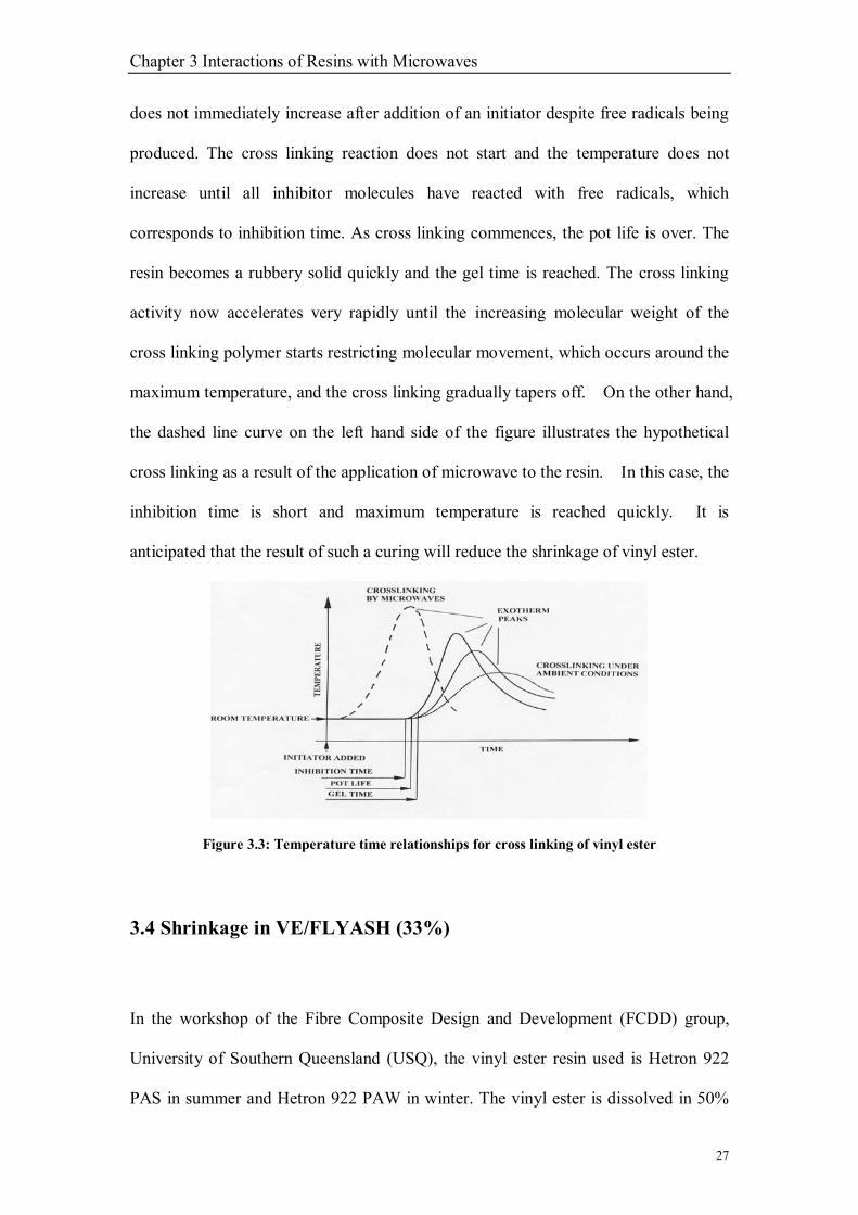
Figure 3.2 shows typical temperature time relations for cross linking of a vinyl ester
following addition of initiator. The three solid curves on the right hand side of the
figure represent room temperature cross linking of vinyl esters.

Chapter 3 Interactions of Resins with Microwaves
26
Figure 3.2: Schematic of addition or free radical cross linking of vinyl ester
The different curves illustrate different amount of initiator, inhibitor, accelerator or
volume of resin. A reduced amount of initiator and accelerator, as well as an increased
amount of inhibitor, leads to later cross linking at lower temperature, and vice versa.
The larger the volume of the resin, the faster the reaction will be. The temperature
Chapter 3 Interactions of Resins with Microwaves
27
does not immediately increase after addition of an initiator despite free radicals being
produced. The cross linking reaction does not start and the temperature does not
increase until all inhibitor molecules have reacted with free radicals, which
corresponds to inhibition time. As cross linking commences, the pot life is over. The
resin becomes a rubbery solid quickly and the gel time is reached. The cross linking
activity now accelerates very rapidly until the increasing molecular weight of the
cross linking polymer starts restricting molecular movement, which occurs around the
maximum temperature, and the cross linking gradually tapers off. On the other hand,
the dashed line curve on the left hand side of the figure illustrates the hypothetical
cross linking as a result of the application of microwave to the resin. In this case, the
inhibition time is short and maximum temperature is reached quickly. It is
anticipated that the result of such a curing will reduce the shrinkage of vinyl ester.
Figure 3.3: Temperature time relationships for cross linking of vinyl ester
3.4 Shrinkage in VE/FLYASH (33%)
In the workshop of the Fibre Composite Design and Development (FCDD) group,
University of Southern Queensland (USQ), the vinyl ester resin used is Hetron 922
PAS in summer and Hetron 922 PAW in winter. The vinyl ester is dissolved in 50%

Chapter 3 Interactions of Resins with Microwaves
28
by weight of styrene. The curing rate for Hetron 922 PAS will be slower in winter and
hence Hetron 922 PAW has to be used for this study. They are both based on the
reaction between methacrylic acid and diglycidylether of bisphenol A (DGEBPA).
Suppliers of the raw vinyl ester resins claim that shrinkage in cured vinyl esters is
around 5 to 6 %. However, the engineers in the Fibre Composite Design and
Development (FCDD) group, University of Southern Queensland (USQ) found that
the shrinkage varied from 10 to 12 % for their large components. Lubin (1982) also
claimed the same amount of shrinkage for the resin with 50% by weight of styrene.
In order to estimate the real shrinkage percentage, one experiment was carried out.
Two beakers of 50 milliliters (internal diameter is 44.10 mm) and 200 milliliters
(internal diameter is 74.95 mm) were employed for the experiment. To start with
polyvinyl acetate (PVA) release agent has to be smeared on the inner surfaces of the
beakers to enable the release of the cured vinyl ester at a later stage. From the Table
3.1 has shown the volume of the composites after shrinkage and before shrinkage:
Table 3.1: Comparison of original and final volumes of VE/FLYASH (33%)
Original volume (ml) 600 400 200 50
Final volume (ml) 535.8 363.94 187.2 47.44
Ambient temperature 16 16 20 20
Relative humidity 52 52 19 19
Peak temperature (oC) 143 139 106 85
Gel time (minutes) 60 65 32.5 35
Percentage of shrinkage 10.7 9.02 6.40 5.13
The resin hardener ratio used in the experiment was 98% resin by volume and 2%
hardener (MEKP) by volume. The reinforce was fly ash (ceramic hollow spheres)
Chapter 3 Interactions of Resins with Microwaves
29
particulate and was made 33 % by weight in the cured vinyl ester composite. Thirty
three percent by weight of fly ash in the composite is considered optimum by FCDD
group because the composite will have a reasonable fluidity for casting combined
with a good tensile strength in service. The curing rate of the mixture of resin,
hardener and fly ash will be faster with higher percentage by volume of hardener,
higher humidity and higher temperature. The ambient temperature when the
experiment was carried out was 20 oC and the relative humidity was 19%. The resin is
a colorless liquid and is first mixed with the red hardener. After that the fly ash is
added to the mixture and they are then mixed to give the uncured composite. To
make a volume of 250 milliliters of uncured composite (of 44% by volume of fly ash
or of 33% by weight), the total volume of resin plus hardener = 250 milliliters x 0.56
= 140 milliliters. For a composite with 98% resin and 2% hardener by volume, the
volume of resin required = 140 milliliters x 0.98 = 137.2 milliliters and that of
hardener required is 2.8 milliliters. It is easier to measure mass rather than volume
so 137.2 milliliters of resin is converted to 137 x 1.1 = 151 g of resin, where 1.1 is the
relative density of the resin. Similarly, the mass of hardener required is 2.8 x 1 = 2.8
g, where 1 is the relative density of the hardener. Since the relative density of the fly
ash is 0.7, the mass of the fly ash required = 110 x 0.7 = 77g. After mixing, 200
milliliters of the composite was poured into the beaker with a volume of 200
milliliters and the rest was poured into another beaker. Data of temperature against
time for the beakers were collected. Temperature measurements were carried out
from the top of the beakers at three points around the centre of the beaker and an
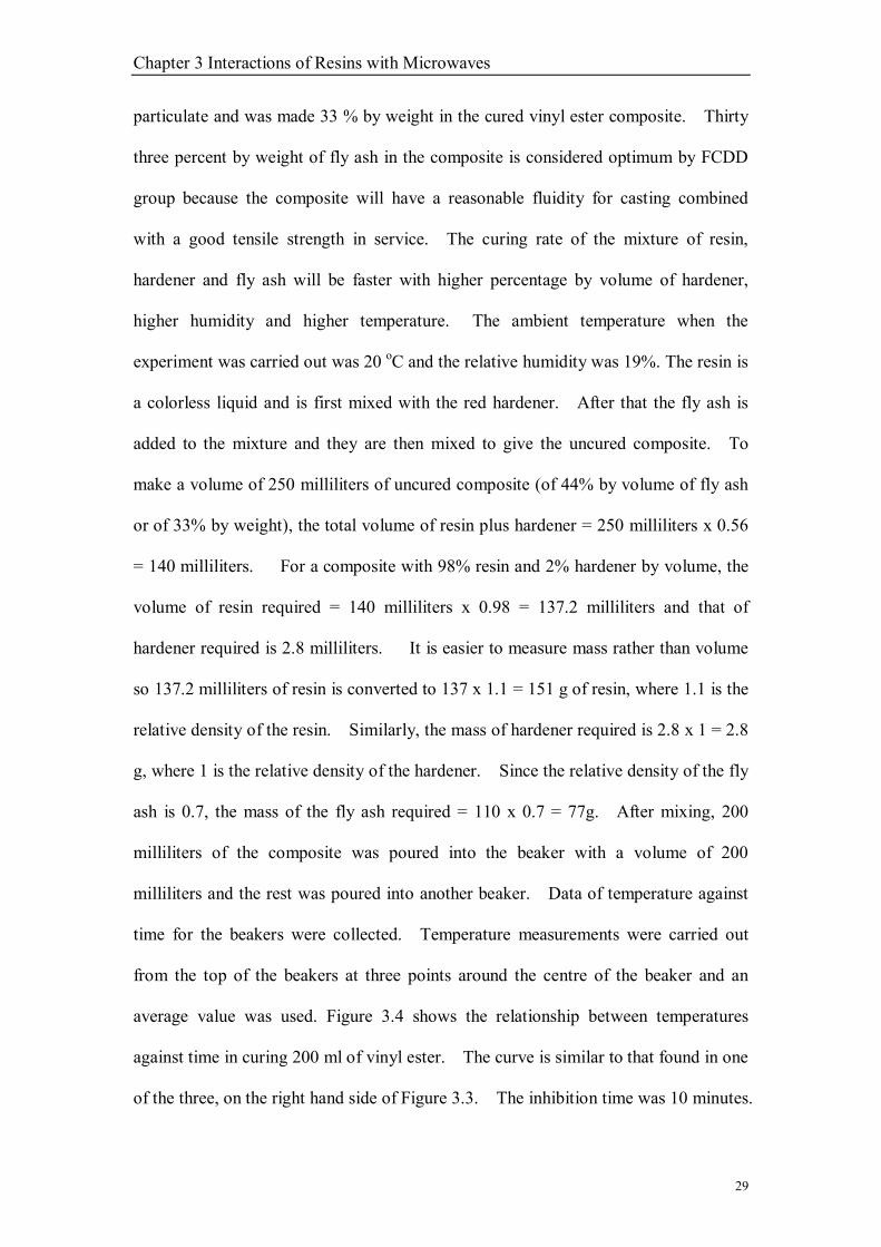
average value was used. Figure 3.4 shows the relationship between temperatures
against time in curing 200 ml of vinyl ester. The curve is similar to that found in one
of the three, on the right hand side of Figure 3.3. The inhibition time was 10 minutes.
Chapter 3 Interactions of Resins with Microwaves
30
At time equaled to 30 minutes, the temperature was 54 oC and a crest was formed on
the surface. At time equaled to 40 minutes, the temperature peaked and was 106 oC.
The temperature then began to drop. Room temperature was regained at time
equaled to 115 minutes. To determine the initial and final volumes of the
composite in the beaker, the height of the level of VE/FLYASH (33%) was measured
by a digital height gauge. The initial height was 48.24 mm, which represents a
volume of 200 ml. Twenty four hours later, the height was re-measured and was
found to be 47.19 mm. The linear shrinkage of the composite after curing was:
0218.024.48
05.124.48
19.4724.48 ==−mm
mmmm
The volumetric shrinkage of the composite can be expressed as (Kalpakjian, 1991):
Vcured = V uncured x3
01
∆−
L
L (Eqn 3.1)
Therefore, Vcured = 200 ml (1-0.0218)3 = 187.20 ml.
The shrinkage is %4.6%100200
20.187200 =− xml
mlml .

Chapter 3 Interactions of Resins with Microwaves
31
Figure 3.4: Relationship between temperature and time in curing 200 ml of vinyl ester composite,
VE/FLYASH (33%) under ambient conditions
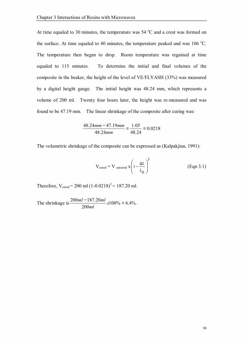
Figure 3.5 illustrates the relationship between temperatures against time in curing 50
ml of vinyl ester. The inhibition time was 10 minutes. A crest was formed at time
equaled to 35 minutes. The temperature peaked at time equaled to 45 minutes and
the temperature was 85oC. Temperature returned to 20oC at time equaled to 95
minutes. The volume was measured by the same method described above after
twenty-four hours (1440 minutes) and it was found that the volume was 47.36 ml. The
shrinkage was 5.28%. From the results of the experiment, it was found that the
larger the volume of vinyl ester, the larger the shrinkage and the higher the peak
temperature would be during curing. This is in line with the historical data kept by
the FCDD group.
Curing 200 ml of VE/FLYASH (33%)
050
100150
0 20 40 60 80 100 120
Time (minutes)
Tem
pera
ture
(o C
)
Chapter 3 Interactions of Resins with Microwaves
32
Figure 3.5: Relationship between temperature and time in curing 50 ml of vinyl ester composite,
VE/FLYASH (33%)
Figure 3.6: Degree of cure of vinyl ester at different curing temperatures
Chapter 3 Interactions of Resins with Microwaves
33
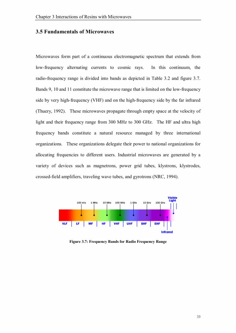
3.5 Fundamentals of Microwaves
Microwaves form part of a continuous electromagnetic spectrum that extends from
low-frequency alternating currents to cosmic rays. In this continuum, the
radio-frequency range is divided into bands as depicted in Table 3.2 and figure 3.7.
Bands 9, 10 and 11 constitute the microwave range that is limited on the low-frequency
side by very high-frequency (VHF) and on the high-frequency side by the far infrared
(Thuery, 1992). These microwaves propagate through empty space at the velocity of
light and their frequency range from 300 MHz to 300 GHz. The HF and ultra high
frequency bands constitute a natural resource managed by three international
organizations. These organizations delegate their power to national organizations for
allocating frequencies to different users. Industrial microwaves are generated by a
variety of devices such as magnetrons, power grid tubes, klystrons, klystrodes,
crossed-field amplifiers, traveling wave tubes, and gyrotrons (NRC, 1994).
Figure 3.7: Frequency Bands for Radio Frequency Range

Chapter 3 Interactions of Resins with Microwaves
34
Table 3.2: Frequency Bands for Radio Frequency Range
Band Designation Frequency limits 4 VLF very low frequency 3 kHz - 30 kHz 5 LF low frequency 30 kHz - 300 kHz 6 MF medium frequency 300 kHz - 3 MHz 7 HF high frequency 3 MHz - 30 MHz 8 VHF very high frequency 30 MHz - 300 MHz 9 UHF ultra high frequency 300 MHz - 3 GHz
10 SHF super high frequency 3 GHz - 30 GHz 11 EHF extremely high
frequency 30 GHz - 300 GHz
Frequency bands reserved for industrial applications are 915 MHz, 2.45 GHz, 5.8
GHz and 24.124 GHz. At the customary domestic microwave frequency of 2.45
GHz, the magnetrons are the workhorse. Material processing falls into this category
(NRC, 1994). Magnetrons are the tubes used in conventional microwave ovens found
almost in every kitchen with a power of the order of a kilowatt. Industrial ovens with
output to a megawatt are not uncommon. Huge sums of money and effort have been
spent in developing microwave-processing systems for a wide range of product
applications. Most applicators are multimode, where different field patterns are
excited simultaneously.
3.6 Microwave and material interactions
The material properties of greatest importance in microwave processing of a dielectric
are the complex relative permittivity ε = ε′ - jε″ and the loss tangent, tan δ = ε″/ ε′
(Metaxas and Meredith, 1983). The real part of the permittivity, ε′, sometimes called
the dielectric constant, mostly determines how much of the incident energy is reflected
at the air-sample interface, and how much enters the sample. The most important
property in microwave processing is the loss tangent, tan δ or dielectric loss, which

Chapter 3 Interactions of Resins with Microwaves
35
predicts the ability of the material to convert the incoming energy into heat. For
optimum microwave energy coupling, a moderate value of ε′, to enable adequate
penetration, should be combined with high values of ε″ and tan δ, to convert microwave
energy into thermal energy. Microwaves heat materials internally and the depth of
penetration of the energy varies in different materials. The depth is controlled by the
dielectric properties. Penetration depth is defined as the depth at which approximately
e1 (36.79%) of the energy has been absorbed. It is also approximately given by
(Bows, 1994):
εε′′′
=
fDp
8.4 (Eqn 3.2)
Where Dp is in cm f is in GHz and ε′ is the dielectric constant.
Note that ε′ and ε′′ can be dependent on both temperature and frequency, the extent of
which depends on the materials. The results of microwaves/materials interactions are
shown in Figure 3.8.
Figure 3.8: Interaction of Microwaves with Materials

Chapter 3 Interactions of Resins with Microwaves
36
During microwave processing, microwave energy penetrates through the material.
Some of the energy is absorbed by the material and converted into heat, which in
turn raises the temperature of the material such that the interior parts of the
material are hotter than its surface, since the surface loses more heat to the
surroundings. This characteristic has the potential to heat large sections of the
material uniformly. The reverse thermal effect in microwave heating does
provide some advantages. These include:
• Rapid heating of materials without overheating the surface
• A reduction in surface degradation when drying wet materials because of lower
surface temperature
• Removal of gases from porous materials without cracking
• Improvement in product quality and yield
• Synthesis of new materials and composites

Chapter 4 Fracture Mechanics
37
Chapter 4
Fracture Mechanics
4.1 Description of Fracture Mechanics
Fracture mechanics can be defined as a field of solids mechanics that deal with the
behaviour of cracked bodies subjected to stresses and strains. Determine the severity of
a pre-existing defect in term of its tendency to initiate a fracture which would cause
failure is the aims of fracture mechanics.
4.2 Fracture Toughness
Typical fracture toughness test can be carry out by applying a tensile stress to a
specimen prepared with a flaw of known size and geometry which is shows in Figure
4.1. The stress applied to the material is increasing at the flaw, which it acts as a stress
raiser. The stress intensity factor K for a simple test calculation is shown as below:
K=f σ√πa (Eqn 4.1)
Where f = geometry factor for the specimen and flaw
σ = the applied stress
a = the flaw size which defined in figure 4.1
If the specimen assumed to have an �infinite� width then it calculate as f ≅ 1.0.

Chapter 4 Fracture Mechanics
38
Figure 4.1: A specimen note that the entire crack length is equal to 2a
By carry out a test on the specimen with known flaw size, the value of k that causes
the flaw to grow and cause failure can be determined. The critical stress intensity
factor was defined as fracture toughness Kc is the K, which required for a crack to
propagate.
When specimen thickness is much greater than the crack dimension, fracture
toughness will depend on the thickness of the sample. The fracture toughness Kc will
Chapter 4 Fracture Mechanics
39
be then decreased to a constant value. Plane strain fracture toughness KIC is what the
constant named. It is KIC that is normally cited for most situations as the property of a
material. The critical fracture toughness value, KIC can improve the reliability of a
structure or component. The ability of a material to resist the growth of crack
propagation based on several factors:
• The ability of the large flaws to reduce its permitted stress
It can be done by using the special manufacturing techniques, such as filtering
impurities from liquid metals and hot pressing of particles to produce ceramic
components. It can help to reduce the flaw size and improve the fracture
toughness.
• The ability of a material to distort is critical
In ductile metals, the material close to the tip of the flaw can be distorted. It is
causing the tip of any crack to become blunt, reducing the stress intensity factor,
and preventing growth of the crack. The increasing strength of a given metal
usually decreases ductility and gives lower fracture toughness. The fragile
materials such as ceramics and polymers have lower fracture toughness than
metals.
• Thicker and rigid materials
These two kinds of materials have lower fracture toughness than thin materials.
• Increasing the rate of application of the load
This application as in an impact test, typically reduces the fracture toughness of
the material.
Chapter 4 Fracture Mechanics
40
• Increasing the temperature will normally increase its fracture toughness
as in the impact test
• A small grain size will normally improve its fracture toughness
This is where more points are defected and dislocations reduced its fracture
toughness. Hence, a fine-grained ceramic material may provide improved
resistance to crack growth.
4.3 The Role of Fracture Mechanics
Design and select material that deal with the behaviour of cracked bodies subjected to
stress and strains was the role of fracture mechanics. Fracture mechanics was an
important tool that let structural engineers to have a better understanding of concrete
structure behaviour, a better design concrete structures and lighter concrete mixture.
The property of the material (KC or KIC), the stress σ that the material must withstand,
and the size of the flaw a must be considered. We can get the third variable once we
figure another two of these variables.
The roles of fracture mechanics been explained as in several steps as below (Donald R.
Askeland, 1996):

Chapter 4 Fracture Mechanics
41
! Selection of a material:
If we know the maximum size a of flaws in the material and the magnitude of the
applied stress, we can still choose a material that has a fracture toughness KC or
KIC large enough to prevent the flaw from growing.
! Design of a component:
If we know the maximum size of any flaw and the material (and therefore its KC
or KIC) has already been selected, we can calculate the maximum stress that the
component can withstand. Then we can design the appropriate size of the part to
ensure that the maximum stress is not exceeded.
! Design of a manufacturing or testing method:
If the material has been selected, the applied stress is known, and the size of the
component is fixed, we can calculate its fracture toughness
4.4 Theories of Mechanics and Fracture Toughness
The development of the field of fracture mechanics was lead by the modifications to
Griffith�s theory. Fracture mechanics deals with facture initiation and crack
propagation, and provides quantitative methods for characterizing the behavior of an
intact material as it fractures due to crack growth. The extension of fracture
mechanics to rock is understandable since rock masses contain cracks and
discontinuities. States of stress around these flaws cannot be predicted using
macroscopic failure criteria. In order to deal with crack propagation, particularly in

Chapter 4 Fracture Mechanics
42
terms of �intentional� fracturing as in size reduction processes, fracture mechanics
must be used.
Although fracture mechanics has an undeniable place in mechanics applications, it
was not developed for geomaterials. It should be recognized that differences exist
between fracture mechanics for man-made materials (metals) and rock fracture
mechanics, particularly in basic material response and engineering application.
Whittaker (et al., 1992) gave a comprehensive list and explanation of these
differences, which can be summarized as:
i. Stress state � Many rocks structures are subjected to compressive stresses as
opposed to tensile stresses. However, in comminution and crushing the induced
stress state is tensile (from point-load compression) and thus tensile fracture is
seen in rock.
ii. Rock fracture � Rock materials usually fracture in a brittle or quasi-brittle
manner and usually do not exhibit plastic flow.
iii. Fracture process zone (FPZ) � Non-elastic behavior ahead of a crack tip in rock
takes the form of micro-cracking as opposed to excessive shear stresses and the
resultant plastic process zone seen in metals. If the size of the FPZ is small then
linear elastic fracture mechanics applies.

Chapter 4 Fracture Mechanics
43
iv. Crack surface � Crack surfaces in rock can be non-planar with friction and
inter-locking occurring, but linear elastic fracture mechanics assumes that no
forces are transmitted across the surface of a smooth planar crack
v. Crack propagation � In rocks there is a tendency for crack propagation to
�wander� along grain boundaries or planes of weakness. The area of newly
created surface is then larger then the assumed fracture area.
vi. Rock fracture mechanics applications � In rock mechanics, as in (man-made)
materials engineering, the prevention of failure by fracture growth is a concern.
But the optimizing the generation and propagation of cracks is also a concern as
in size reduction processes. Thus the application dictates how material parameters
should be determined and used.
vii. Influence of scale � Due to the complicated geologic nature of rock masses, the
characterization of a rock mass is high. For the prevention of crack growth and
failure, parameters measured experimentally are of secondary importance but for
rock fragmentation applications, experimentally measured properties are of
primary importance.
viii. Heterogeneity � Changes in local structure and strength ahead of a crack tip
affects the continuity of crack growth.
ix. Presence of discontinuities � Pre-existing discontinuities affect the local stress
states and crack propagation.

Chapter 4 Fracture Mechanics
44
x. Anisotropy � Rocks can be anisotropic affecting measured fracture parameters as
a function of crack orientation.
There are more practical and developed concepts of fracture mechanics was lead by
the recognition of these variations as it applies to behavior, with principles of linear
elastic fracture mechanics being extended even to rocks that behave non-linearly and
much of the focus centering on the measurement of fracture toughness.
The most fundamental aspect of rock fracture mechanics is the establishment of a
relationship between rock fracture strength and the geometry of the flaws that result in
fracture. Through this relationship an intrinsic material property that describes a
materials� resistance to crack propagation can be measured. This property is called
fracture toughness. The application of fracture toughness in size reduction processes
is clear. Fracture toughness represents a critical level above which crack extension
and fracture occurs. When individual rock particles are subjected to the applied forces
of size reduction, it is most likely that the intrinsic tensile property measured as the
fracture toughness will control breakage (Bearman, 1998). Since the amount of
energy input into a size reduction process and the amount of size reduction achieved
(i.e., the fractured size distribution) are related to the type of loading and the crack
pattern in the material, there should be a relationship between these parameters and
fracture toughness.
4.5 Transition Temperature Approach
The transition temperature approach assumes that every material below a certain
temperature will become brittle. This is caused by the material not being able to

Chapter 4 Fracture Mechanics
45
plastically yield so that the stress concentration at the crack tip can not be absorbed
thus causing it to fracture a lower stress. Figure 4.2 shows the general effect of
temperature of the fracture resistance of structural metal.
Figure 4.2: The general effect of temperature of the fracture resistance of structural metal
Various tests are used to determine the transition temperature of a material .The
transition temperature is difficult to accurately find so a range of temperatures are
used, these ranges of results are grouped into general categories (Osgood, 1971):
# Fracture-stress Transition temperature:
At this point the fracture strength of sharp- notched specimen decreases rapidly
well below the yield strength
# Fracture-mode Transition Temperature:
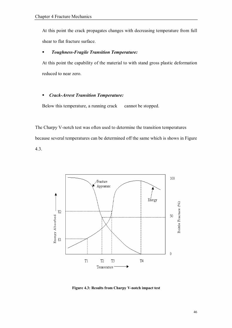
Chapter 4 Fracture Mechanics
46
At this point the crack propagates changes with decreasing temperature from full
shear to flat fracture surface.
# Toughness-Fragile Transition Temperature:
At this point the capability of the material to with stand gross plastic deformation
reduced to near zero.
# Crack-Arrest Transition Temperature:
Below this temperature, a running crack cannot be stopped.
The Charpy V-notch test was often used to determine the transition temperatures
because several temperatures can be determined off the same which is shows in Figure
4.3.
Figure 4.3: Results from Charpy V-notch impact test

Chapter 4 Fracture Mechanics
47
T1 � From fixed level of impact energy T2 - Fracture resistance T3 � Midpoint temperature T4 � Fracture entirely sheer
The transition temperatures are compared with fracture resistance of other materials,
which are considered for the design. The material with the lowest transition
temperature is considered to be the most fracture resistant.
This method is determining fracture resistance, the results cannot be expressed directly
in terms of load-carrying term but with use of a fracture analysis diagram applied stress,
defect size and temperature can be related. Figure 4.4 show the fracture analysis
diagram
Figure 4.4: Fracture analysis diagram

Chapter 4 Fracture Mechanics
48
4.6 Linear Elastic Fracture Mechanics
2'saEσπ=γ (Eqn 4.2)
.
Above equation presented as a size independent expression characterizing the
resistance of a material to fracture based on the stresses required for breakage and the
presence of flaws. It showed that fracture initiation in a brittle solid is controlled by
the product of a far-applied stress and the square root of the flaw length which reaches
a critical value determined by the characteristic material properties E, ν, and γs. This
critical value is called the critical stress intensity factor and is denoted Kc. Irwin (1957)
used a stress intensity approach to relate the critical strain energy release rate Gc to the
critical stress intensity factor Kc. Rather than follow Griffith�s global approach, Irwin
considered the crack tip region, which is small compared to the rest of the body but
large enough with respect to atomic dimensions such that linear elastic theory applies
(Knott, 1972). Irwin determined the work required to close up a small portion of a
crack by superimposing tensile forces along the crack surfaces and hypothesized that
this work is equal to the energy released when the crack extends. Thus the work
required to close a unit length of the crack is the strain energy release rate and, based
on the stresses and displacements occurring as a result of the tensile forces, is equal
to:
EKvG
22 )1( −= (Eqn 4.3)
Since crack propagation occurs when G reaches a critical value, the critical value of
stress intensity can be defined as:

Chapter 4 Fracture Mechanics
49
)1( 2vEG
K cc −
= (Eqn 4.4)
By demonstrating the equivalence of K and G, Irwin provided the basis for the
development of Linear Elastic Fracture Mechanics (LEFM). In LEFM the crack tip
stresses, strains, and displacements can be characterized by K as long as inelastic
yielding ahead of the crack tip is small. The advantage of LEFM is that it provides a
universal approach for determining a material�s resistance to fracture, as defined by
Kc. As long as an explicit function for the stress intensity near a crack tip is known for
a given crack geometry and loading configuration, Kc can be measured
experimentally.
4.7 Stress Intensity Factor
Severity of the crack condition as affected by crack dimension, stress, and geometry is
mention by stress intensity factor K in previous section(Dowling, 1999). Determining
K is based on a linear-elastic approach (hence LEFM), which assumes the material in
which the crack is located is isotropic and behaves according to Hooke�s Law.
Different loading configurations at a crack tip lead to different modes of crack tip
displacement. The different types of crack deformation are generalized using three
basic modes. Mode I is the opening mode due to tension, where the crack surfaces
move directly apart; Mode II is the sliding mode due to shearing, where the crack
surfaces move over one another in a direction perpendicular to the crack front; Mode
III is the tearing mode also due to shearing, where the crack surfaces sliding over one
another but in a direction parallel to the crack front. The three basic modes can also
occur in combination as �mixed-mode� loading with the superposition of the modes
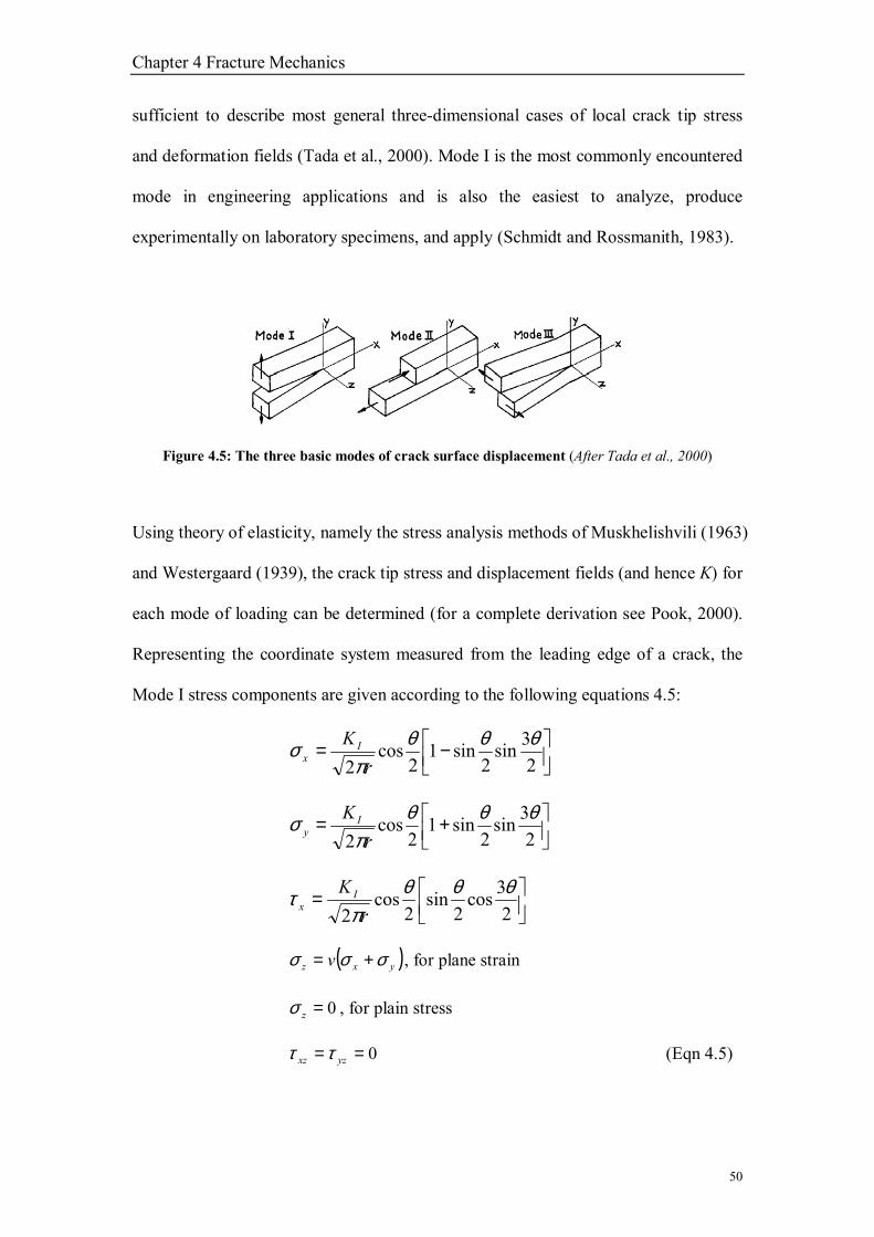
Chapter 4 Fracture Mechanics
50
sufficient to describe most general three-dimensional cases of local crack tip stress
and deformation fields (Tada et al., 2000). Mode I is the most commonly encountered
mode in engineering applications and is also the easiest to analyze, produce
experimentally on laboratory specimens, and apply (Schmidt and Rossmanith, 1983).
Figure 4.5: The three basic modes of crack surface displacement (After Tada et al., 2000)
Using theory of elasticity, namely the stress analysis methods of Muskhelishvili (1963)
and Westergaard (1939), the crack tip stress and displacement fields (and hence K) for
each mode of loading can be determined (for a complete derivation see Pook, 2000).
Representing the coordinate system measured from the leading edge of a crack, the
Mode I stress components are given according to the following equations 4.5:
−=
23sin
2sin1
2cos
2θθθ
πσ
rK I
x
+=
23sin
2sin1
2cos
2θθθ
πσ
rK I
y
=
23cos
2sin
2cos
2θθθ
πτ
rK I
x
( )yxz v σσσ += , for plane strain
0=zσ , for plain stress
0== yzxz ττ (Eqn 4.5)

Chapter 4 Fracture Mechanics
51
where KI is the stress intensity factor for Mode I. The displacements at the crack tip
can be found by substituting above equation into Hooke�s Law.
Figure 4.6: Coordinate system for a crack tip
It can be seen from Equations 4.5 that at the crack tip (as r approaches zero) the
stresses approach infinity, as has already been indicated by Inglis� solution for
stresses around an elliptical hole in a stressed plate. Since no value of stress at the
crack tip can be given, and all non-zero stresses of Equation 4.5 are proportional to KI,
with the remaining factors varying only with r and θ, the stress field near the crack tip
can be determined by giving the value of KI, which has a formal definition of
(Dowling, 1999; Pook, 2000):
rK yorI πσθ 2lim , →= (Eqn 4.6)
It was noted earlier that KI is affected by the crack size, stress, and geometry. In order
to account for different geometries Equation 4.6 can be rewritten as:

Chapter 4 Fracture Mechanics
52
aFK I πσ 2= (Eqn 4.7)
where, F is a dimensionless constant dependent on the geometric configuration
σ is the stress averaged over the gross area a is the half-crack length. F can generally
be described as a function of loading geometry and aw where w is defined as the
maximum possible crack length. When F is determined for a given geometry the
critical value of stress intensity, or fracture toughness, can be determined as long as
inelastic yielding ahead of the crack tip is small and the conditions for LEFM are met.
Equations and values of F for a wide range of crack, specimen, and loading
geometries are determined using analytical, numerical, and experimental methods and
have been compiled in various handbooks (see Tada et al., 2000; Murakami, 1987;
Rooke and Cartwright, 1976; Sih, 1973).

Chapter 5 Tests of Fracture Toughness
53
Chapter 5
Tests of Fracture Toughness
5.1 Description of Fracture Toughness Tests
The KIC (fracture toughness) can define as material of a sharp crack that has the
characteristics of its resistance to fracture under tensile conditions. It is extremely
important property in many crucial design applications. The crack will automatically
become unstable and it will propagate quickly until fracture occurs when the stress
intensity factor grows and becomes higher than KIC.
Plane strain is the term when the stress state is characterized with thick or bulky parts
for which the stress of the flaw is in triaxial tension. However, the material usually
fails in a brittle manner when it is in plane strain conditions. In plane strain conditions,
if the stress intensity factor exceeds its critical value, the flaw will propagate
unexpectedly and run completely through the section.
Plane stress condition is related to all sections of two-dimensional parts which is the
most complicated stress can occur and known as biaxial. Consequently, the flaw in
plane stress will grow slowly until it is below the increased stress. It will then
propagate unexpectedly and total fracture occurs.
The basic concepts of crack growth explained why the plane stress leads to slow
fracture and why the plane strain leads to rapid fracture. Hence, it is the reason that

Chapter 5 Tests of Fracture Toughness
54
the plane strain fracture toughness KIC is known as such an important property in
fracture prevention.
There are several kinds of different testing methods that can be used to determine the
fracture toughness, KIC. The following sections will briefly explain some of the
standard and non-standard testing procedures.
5.2 Standard Test Methods
United States of America (USA) and United Kingdom (UK) have adopted two similar
testing procedures for determining KIC. These tests are documented in The American
Standard ASTM: E339 and the British Standard BS: 5447. All standard tests have
there supposed dimensions for the different specimens recommend by their relevant
standards. All the specimens have a single edge notches that ate initiated by low stress
fatigue cracking.
5.2.1 Compact Tensile Specimen
The compact tension is a flat plate with single notch, which is fatigue cracked (Figure
5.1). The load is applied throughout two pins in line with the crack tip. As the result,
this causes the two-point load onto the specimen. Figure 5.1 show the compact tensile
specimen.

Chapter 5 Tests of Fracture Toughness
55
Figure 5.1: Compact tensile specimen
5.2.2 C-Shape Specimen
The purpose of C-shaped specimens is to check on portions of hollow cylinders. The
C-shaped specimens have a single notch mid-center of arc which is fatigue cracked.
The specimen is loaded throughout pins in two-point bending. Figure 5.2 shos the
C-shape specimen.
Figure 5.2: The C-shape specimen

Chapter 5 Tests of Fracture Toughness
56
5.3 Non-Standard Test Methods
Due to the cost and size of the sample required in the standard test, these type of tests
were developed which is shown as Figure 5.3 for Charpy V-notch test rig and sample
and Figure 5.4 for short rod specimen configuration and dimensions.
These types of tests are considered as non-standard tests, and the data from these tests
which tell the mechanical properties of the material and there are related to the
fracture toughness.
5.3.1 Charpy V-Notch Test
Figure 5.3: Charpy V-notch test rig and sample
The Charpy V-notch test is used to determine the resistance of the material to crack
propagation. In this test, the impact energies are measured with reverence to the

Chapter 5 Tests of Fracture Toughness
57
temperature. The following two equations can be used to relate the impact test to
fracture toughness in order to determine the KIC value of a material:
KIC2
=2 E (CVN) 3/2 (Eqn 5.3.1.2)
KIC2= 8 E (CVN) (Eqn 5.3.1.3)
The Charpy V-Notch (Cv-NDT) test is associated to the impact energy Cv. that is also
associated to the nil-ductility transition temperature. The Cv energy does not
correspond directly to the NDT level of fracture resistance. This make the value of Cv
is unique for each type of steel; a correlation value should always be used. The
V-notch impact test values are generally suitable for correlation with fracture
toughness values.
5.3.2 Short Bar Test
Barker (1977) started to work on the concept of devising a simplified method to
measure plane strain fracture toughness. The simplified method used small rod and
bar shape specimens, that will be cracked fracjack mechanism or by other test rigs.
The test is started with an opening load (F) applied to the mouth of the specimen. This
causes a fracture to initiate at the point of the chevron. The constant widening of the
crack front, as it evolved along the axis of the specimen can causes stable crack
growth, even in brittle materials. Hence, a "real" crack is created in the specimen
before the toughness measurement is made.
For Linear Elastic Fracture Mechanics (LEFM) materials, the fracture toughness
measurement is made at the time of maximum load. It is made when the crack is in the
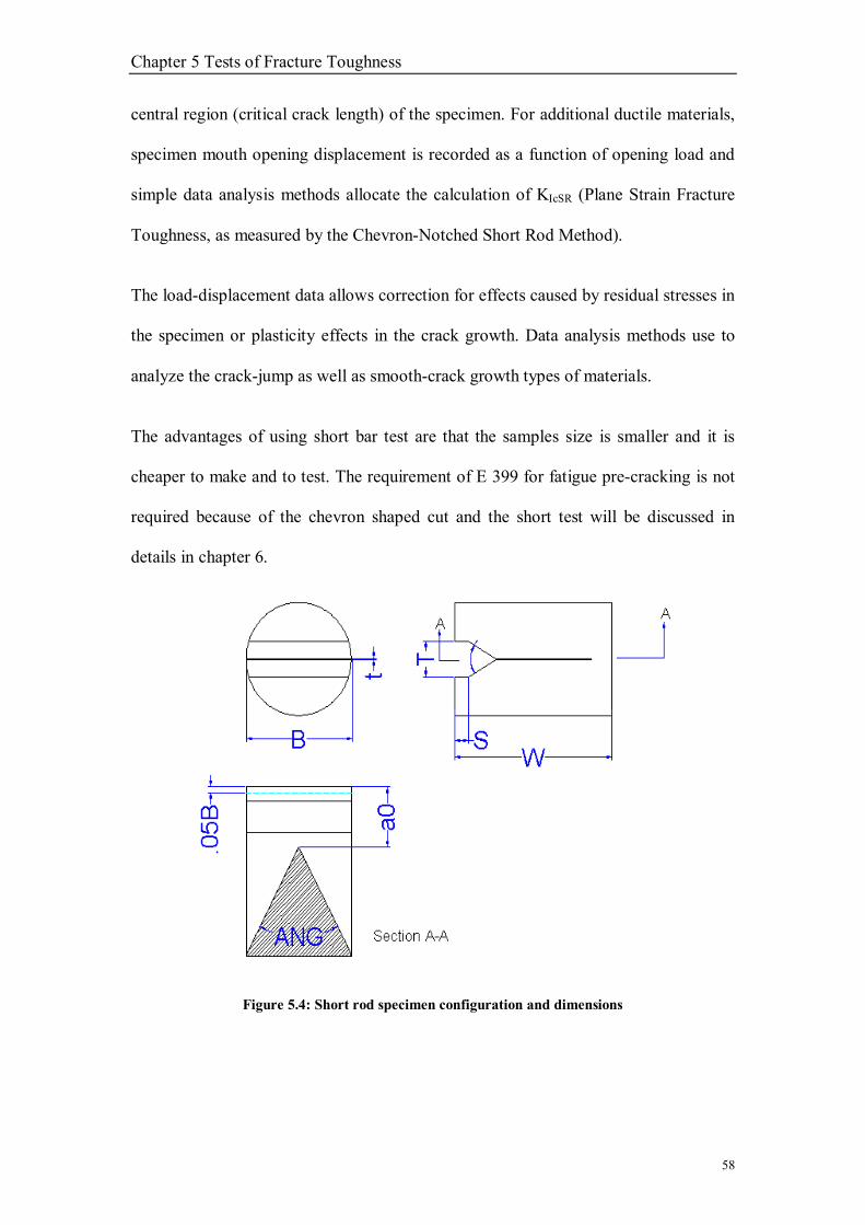
Chapter 5 Tests of Fracture Toughness
58
central region (critical crack length) of the specimen. For additional ductile materials,
specimen mouth opening displacement is recorded as a function of opening load and
simple data analysis methods allocate the calculation of KIcSR (Plane Strain Fracture
Toughness, as measured by the Chevron-Notched Short Rod Method).
The load-displacement data allows correction for effects caused by residual stresses in
the specimen or plasticity effects in the crack growth. Data analysis methods use to
analyze the crack-jump as well as smooth-crack growth types of materials.
The advantages of using short bar test are that the samples size is smaller and it is
cheaper to make and to test. The requirement of E 399 for fatigue pre-cracking is not
required because of the chevron shaped cut and the short test will be discussed in
details in chapter 6.
Figure 5.4: Short rod specimen configuration and dimensions

Chapter 5 Tests of Fracture Toughness
59
5.4 Analysis of Fracture
Figure 5.5: The instruments magnification ranges
Fractured surfaces show both macroscopic and microscopic features, where a wide
range of instruments with varying magnifications are required. Figure 5.5 shows the
magnification ranges, which the certain instruments are effective.
Macroscopic test of the fractured surface have to be completed first, as this can be
done with the naked eye or a hand lens. This usually indicates the crack origins and
the direction of crack growth. In recent failures, the mode of failure can sometimes be
distinguished as the surface has not begun to corrode.
When the site of the crack nucleation is identified, a stereomicroscope is the most
useful tool to examine the crack origin for notable features as this could assist in the
determination of the mode of fracture.
The Scanning Electron Microscope (SEM) is a very useful tool to examine the
fracture surfaces. The advantages of this SEM is because it has a large depth of field
Chapter 5 Tests of Fracture Toughness
60
and has a wide range of working magnification from low to high magnifications. The
SEM has virtually replaced the optical microscope for direct examination of fractured
surfaces.
The Transmission Electron Microscope (TEM) is very useful tool in the field of
fractography due to its fracture surface details that can be studied at very high
magnifications (up to x100, 000). There are two disadvantages of TEM; it is time
consuming and it needs required skills to prepare samples that would be useful.
5.4.1 Brittle Fracture
Brittle fractures generally occur with slight plastic deformation. The strain rates
within the material are regularly high because of the stress systems. Brittle fractures
occur with little warning because the crack knows how to grow at the speed of sound.
Excessive overloading or an impact force can cause a brittle fracture.
Macroscopic analysis of a brittle material failure shows that the materials fail
differently which depends on whether it was in tension or compression. When the
material fails in tension, the crack is perpendicular to the applied load. If the sample
fails in compression the fracture will occur at 45 degrees to the applied load.
The crack is usually initiated from flaws of the material; these can be caused by either
surface finish or impurities within the material. The cracks can be intergranular or
transgranular depending on the material. A truly brittle fracture is caused by cleavage,
Chapter 5 Tests of Fracture Toughness
61
which means transgranular. Cleavage occurs when the material is under high
constraint conditions (Baddeley, D T and Ballard J, 1991).
5.4.2 Ductile Fracture
A ductile fracture is the result of plastic deformation prior to failure. A ductile
fracture usually occurs when the sample is in strain. Overloading usually causes
ductile transgranular fractures. It can be sometimes recognized from macroscopic test
of the failed specimen. Usually the specimen is thin size and there is contraction of
the sample before failure occurs.
At a microscopic level, most of the structural materials fail by a process called
microvoid coalescence. Microvoid coalescence caused the fractured surface to have a
dimple appearance with both large and small dimples. The shape of the dimple is
influenced by the type of loading which is applied to the sample. Failures caused by
shear will produce extended shaped dimples that point in the opposite directions on
the matching fracture surfaces. Tensile tearing produces extended dimples that point
in the same direction on matching fracture surfaces (Baddeley, D T and Ballard J,
1991).

Chapter 6 Short Bar Test
62
Chapter 6
Short Bar Test
6.1 Standard Tests
There are currently two similar testing procedures for determine Kic which are used
by United States of America and the United Kingdom. These tests were documented
in the ASTM (Americans Standard Test Method) and the BS (British Standards
Institution Test Method). All standard tests have there supposed dimensions for the
different specimens recommend by their relevant standards. All the specimens have a
single edge notches that ate initiated by low stress fatigue cracking.
6.2 Non Standard Tests
Except both of Charpy V- notch test and Short rod/ bar test, there are several other
tests that are considered as non-standard tests, the data from these tests which tell the
mechanical properties of the material and there are related to the fracture toughness.
These type of tests were developed due to the cost and size of the sample required in
the standard test.

Chapter 6 Short Bar Test
63
6.2.1 Short Bar Test
Since the fracture toughness of a material is an important property, which is vital in
design applications. The valid measurement of Kic only can determine by using
ASTM and BS standard tests; however, there are many disadvantages for these
standards, such as:
• Example like a sufficiently large specimen, it will preclude the fracture toughness
measurement, due to the size of specimen required by the standard is too large, it
cannot be removed from the structure of interest.
• As the size of specimen required, the size of tensile machine is also very large
which means that the availability of machine is limited and it will cost much in the
testing as well.
• Some material properties such as brittleness and high fracture toughness combined
with low yield strength sometimes makes it impossible to meet the specimen
requirements of the standard tests.
• The fatigue pre-cracking which is required of the samples.
• The difficulties in measuring the crack length.
• Lastly, the overall cost of testing one sample is very expensive.

Chapter 6 Short Bar Test
64
An alternative test method was considered, which was less complex and applicable to a
wider range of materials. The short bar test was developed by Barker in 1977. And he
considered that the test samples should exhibit some crack growth stability. His testing
method used simple fracture toughness concepts to test sample configurations
exhibiting crack growth even when loaded by a controlled force machine.
Once calibrated for specimen configurations, the only parameter required for fracture
toughness values was the peak force required to completely fracture the sample. This
new test method used samples of a circular of rectangular cross section, which were
called short rod/bar samples accordingly (Barker, 1977). On the other hand, the
advantages of short bar test were (DiJon Inc, Technical note 503):
• No fatigue pre-cracking was required therefore the method was applicable to
brittle as well as ductile materials.
• No load versus deflection graph required.
• No crack position or crack length measurements required.
• The size of specimen for a valid test has been reduced.
Therefore, those advantages are able to bring a reduction in costs of testing equipment
and samples. Therefore, ASTM committee is now considering this method as an
additional specimen configuration for the determination of fracture toughness (Kic).

Chapter 6 Short Bar Test
65
6.3 Selection of the Short Rod or Bar Geometry
The configuration of the short bar specimen was selected on the basis of large number
of tests of specimens with different length-to-diameter ratios and various chevron slot
geometries. The criteria on which the current geometry was selected was:
• The tendency for the crack to �pop� at the initiation should be minimized. The
crack initiation should be as smooth as possible.
• The crack should tend to be well guided by the chevron slot.
• The width of the crack front should be considerable portion of the specimen
diameter at the time of toughness measurement.
• The crack should be near the centre of the specimen (far from both ends) at the
time of the toughness measurement.
• The load should be at or near its peak value at the time of toughness measurement.
• The specimen geometry should be as simple as possible for ease of fabrication.
• The specimen should economical in its use of sample material.
Some of these criteria could not be achieved and the same time. The short rod and bar
specimen configurations were selected as a reasonable compromise in an attempt for
an optimum geometry. [Baker, 1981]
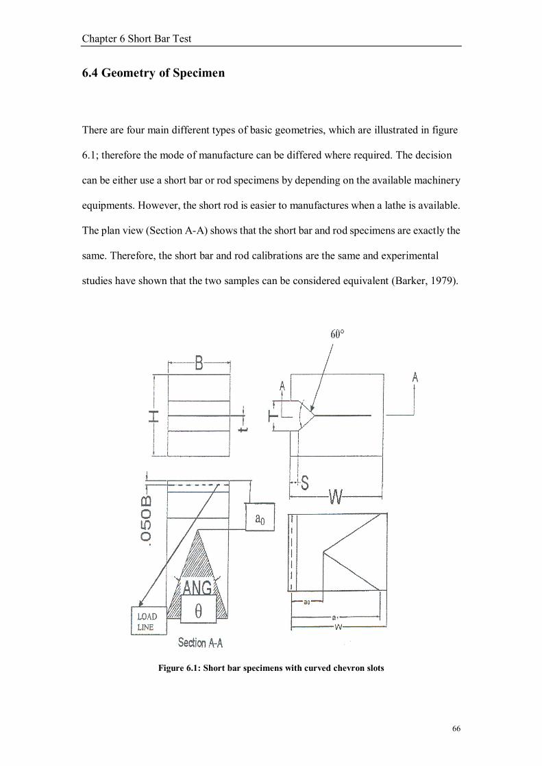
Chapter 6 Short Bar Test
66
6.4 Geometry of Specimen
There are four main different types of basic geometries, which are illustrated in figure
6.1; therefore the mode of manufacture can be differed where required. The decision
can be either use a short bar or rod specimens by depending on the available machinery
equipments. However, the short rod is easier to manufactures when a lathe is available.
The plan view (Section A-A) shows that the short bar and rod specimens are exactly the
same. Therefore, the short bar and rod calibrations are the same and experimental
studies have shown that the two samples can be considered equivalent (Barker, 1979).
Figure 6.1: Short bar specimens with curved chevron slots
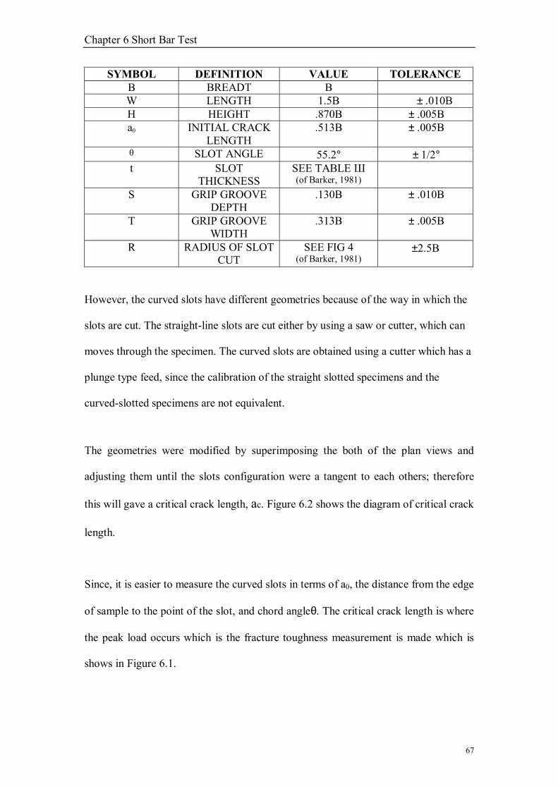
Chapter 6 Short Bar Test
67
SYMBOL DEFINITION VALUE TOLERANCE B BREADT B W LENGTH 1.5B ± .010B H HEIGHT .870B ± .005B a0 INITIAL CRACK
LENGTH .513B ± .005B
θ SLOT ANGLE 55.2° ± 1/2° t SLOT
THICKNESS SEE TABLE Ш (of Barker, 1981)
S GRIP GROOVE DEPTH
.130B ± .010B
T GRIP GROOVE WIDTH
.313B ± .005B
R RADIUS OF SLOT CUT
SEE FIG 4 (of Barker, 1981)
±2.5B
However, the curved slots have different geometries because of the way in which the
slots are cut. The straight-line slots are cut either by using a saw or cutter, which can
moves through the specimen. The curved slots are obtained using a cutter which has a
plunge type feed, since the calibration of the straight slotted specimens and the
curved-slotted specimens are not equivalent.
The geometries were modified by superimposing the both of the plan views and
adjusting them until the slots configuration were a tangent to each others; therefore
this will gave a critical crack length, ac. Figure 6.2 shows the diagram of critical crack
length.
Since, it is easier to measure the curved slots in terms of a0, the distance from the edge
of sample to the point of the slot, and chord angleθ. The critical crack length is where
the peak load occurs which is the fracture toughness measurement is made which is
shows in Figure 6.1.

Chapter 6 Short Bar Test
68
A table of equivalent ac for the versatile a0 and θ are shown in Figure 6.3 diagram,
this is because a constant specimen calibration can be used regardless of specimen
size, when the crack is in the vicinity of the critical crack length, ac.
Figure 6.2: Diagram of critical crack length
Figure 6.3: The equivalence for curved chevron slots
Chapter 6 Short Bar Test
69
The configurations of correction factors were calculated because it is regarding how
sensitive the test results were to variations in a0, 0, W. The test results can be
corrected by multiplying the results by Cc, this only works for specimens, which are
out of tolerance by three times the tolerance limits.
6.5 Short Bar Test Description
With the short bar test, it is not only the specimen geometry and preparation important
in fracture toughness results, but the testing procedure must also be controlled to
obtain valid fracture toughness result.
The short bars tests involve an opening load being applied near the mouth of the
specimen, causing a crack to initiate at the point of the chevron slot. Ideally, the
opening load should be less than the load that will be required to further advance the
crack.
A continually increasing load must be supplied until the crack length reaches the
critical crack length, ac, beyond ac, the load should decrease, shown in Figure 6.4.
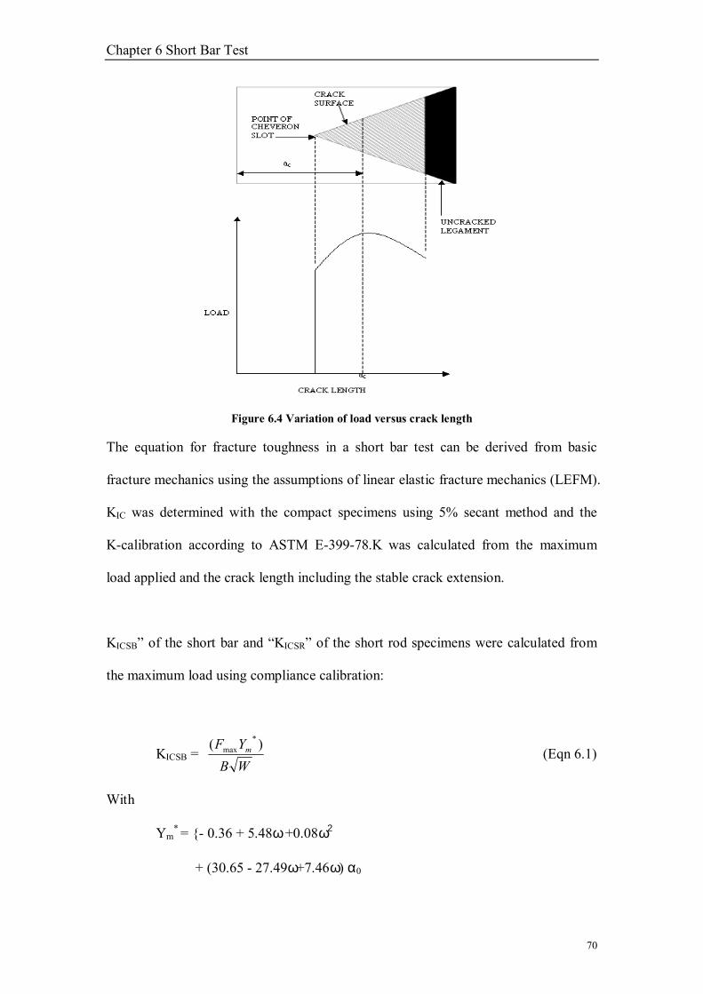
Chapter 6 Short Bar Test
70
Figure 6.4 Variation of load versus crack length
The equation for fracture toughness in a short bar test can be derived from basic
fracture mechanics using the assumptions of linear elastic fracture mechanics (LEFM).
KIC was determined with the compact specimens using 5% secant method and the
K-calibration according to ASTM E-399-78.K was calculated from the maximum
load applied and the crack length including the stable crack extension.
KICSB� of the short bar and �KICSR� of the short rod specimens were calculated from
the maximum load using compliance calibration:
KICSB = WBYF m )( *
max (Eqn 6.1)
With
Ym* = {- 0.36 + 5.48ω +0.08ω2
+ (30.65 - 27.49ω+7.46ω) α0

Chapter 6 Short Bar Test
71
+ (65.90+18.44ω-9.76ω)α02}
21
0
01
1
−−ααα (Eqn 6.2)
KICSR = DBYF m )( *
max (Eqn 6.3)
With
Ym* = {19.98 � 9.54
DW + 6.8(
DW ) 2
+ [� 118.7 + 125.1DW � 22.08 (
DW ) 2] α0
+ [379.4� 363.3 DW + 84.4 (
DW ) 2] α0
2} 21
0
01
1
−−ααα
(Eqn 6.4)
Where, W = Width, H = Height, D = Diameter, B = Breadth
ω = HW , α0 =
Wa0 , α1=
Wa1
Chapter 7 Experiment Method
72
Chapter 7
Experiment Method
7.1 Specimen Preparation
Initially, the dimensions of specimen are accordingly modified to the geometrical
requirements for the standard ISRM short rod or bar test, where the length to diameter
(short rod) or breadth (short bar) ratio, DL =1.45; the range of diameters can only be
varied from test to test in the range of 46 − 92 mm for the tensile test. The choice of
scale is significant for the convenience of fabricating the features of the moulds. The
dimensions of the short bar specimens used was attached in Appendix.
7.2 The Process of Building up the Mould
There are several criteria in preparing the moulds.
• How to recycle the moulds.
• How much will the vinyl ester specimen shrinkage be.
Therefore one has to improve the mould. The following procedures were carried out
in fabricating the moulds:
1. Draft the part and base of the moulds.
2. Converted the draft into computer-aided drawing by using the Auto-CAD
2002 LT. as shown in the figure 7.1

Chapter 7 Experiment Method
73
Figures 7.1: The Auto-CAD drawing for the triangle part of the mould
3. The manila folders were cut according to the figure 7.1.
4. The manila folder being cut was folded and pasted around the plastic mould
with cellophane tape which is shown in figure 7.2.
5. The manila folder part was pasted to the base.
6. The internal view of the complete mould is shown in the figure 7.3

Chapter 7 Experiment Method
74
Figure 7.2: The triangle mould for making the slot and important features of short bar specimen
Figure 7.3: The internal view of short bar specimen mould

Chapter 7 Experiment Method
75
In this study, thanks have to be given to Mr. Robert Davey who designed the mould
and shared it with me.
Steps in preparing the mould for casting:
1. First of all, clean up the surface of the mould nicely and fix it up as shown in
figure 7.4.
Figure 7.4: Explore view of mould
2. Spray canola oil (cooking use) on the inner surface of mould figure 7.5(a) &
figure 7.5(b). For pasting the triangle part, some normal glue with low bonding
strength was used.

Chapter 7 Experiment Method
76
Figure 7.5(a)
Figure 7.5(b)
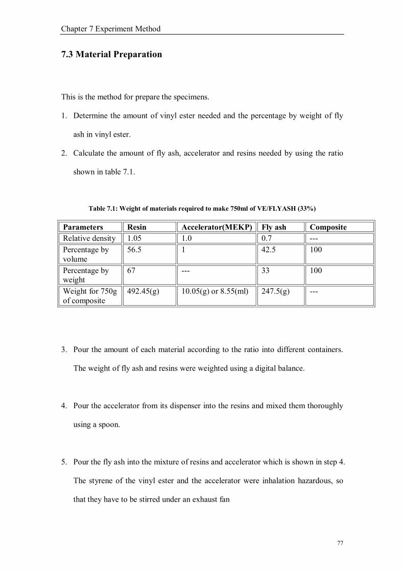
Chapter 7 Experiment Method
77
7.3 Material Preparation
This is the method for prepare the specimens.
1. Determine the amount of vinyl ester needed and the percentage by weight of fly
ash in vinyl ester.
2. Calculate the amount of fly ash, accelerator and resins needed by using the ratio
shown in table 7.1.
Table 7.1: Weight of materials required to make 750ml of VE/FLYASH (33%)
Parameters Resin Accelerator(MEKP) Fly ash Composite Relative density 1.05 1.0 0.7 --- Percentage by volume
56.5 1 42.5 100
Percentage by weight
67 --- 33 100
Weight for 750g of composite
492.45(g) 10.05(g) or 8.55(ml) 247.5(g) ---
3. Pour the amount of each material according to the ratio into different containers.
The weight of fly ash and resins were weighted using a digital balance.
4. Pour the accelerator from its dispenser into the resins and mixed them thoroughly
using a spoon.
5. Pour the fly ash into the mixture of resins and accelerator which is shown in step 4.
The styrene of the vinyl ester and the accelerator were inhalation hazardous, so
that they have to be stirred under an exhaust fan

Chapter 7 Experiment Method
78
6. Pour the mixture into the mould slowly after stirring for a few minutes.
7. Took the material for microwave exposure and cured under the exhaust fan or
leave the material to cure under exhaust fan (for ambient).
7.4 Safety Measures
The safety measures when processing the specimens included risks of styrene, risks of
MEKP and risks on microwaves and vinyl ester resins interaction. Due to these high
risks involved in specimen making, various safety measures must be considered
seriously.
The testing and specimen making were carried out in the Faculty of Engineering and
Surveying, USQ. Before mixing the material, two different kinds of safety gloves
were required to be worn, one after the other. The 1st layer is mainly for protecting
skin and it is thicker and less porous than the 2nd layer. The 2nd layer glove is just for
extra protection.
Goggles were worn for eye protection and it must be worn while mixing the mixture
because the styrene emitted will be harmful to eyes. Besides that, mask was also used
to avoid any inhalation of styrene vapour into the body. The exhaust fan must also be
on during mixing the material. If not, the styrene will always be in the room. The
gloves must be thrown away after use and hands have to be washed before leaving the
room.

Chapter 7 Experiment Method
79
While curing the specimens with microwave, the microwave should be located
outdoor as the styrene go to the open air. Figure 5.5 shows the microwave oven that
is used in this research project. During microwave processing, the door of the
microwave oven should be facing onto a wall to reduce damage in case of explosion.
7.5 Microwave Exposure of Composites
7.5.1 The Modified Microwave Oven
The microwave oven was slightly modified for use in this experiment. The main part
is to direct the styrene gas evolved to exhaust rapidly.
Figure 7.6: The modified oven and its peripherals (Ku, H S 2002b)
Oven Cavity
Exhaust
Pipe

Chapter 7 Experiment Method
80
7.5.2 Type of the Microwave Exposure Time
There are 12 types of conditions for the microwave exposure of the specimens. They
are 180-Watt power with exposure of 60seconds, 70 seconds and 80 seconds, and
360-Watt power with exposure of 60seconds, 70 seconds and 80 seconds, and
540-Watt power with exposure of 15 seconds, 20 seconds and 25 seconds, and
720-Watt power with exposure of 15 seconds, 20 seconds and 25 seconds.
Table 7.2 shows the changes in volume and other parameters of vinyl ester
composites after exposure to the different power levels and exposure times.
Table 7.2: Volume shrinkage and other parameters for 400 ml of VE/FLYASH (33%) exposed to
180-W microwaves at different duration
Microwave exposure time (seconds) 0 55 60 65
Oven cavity Temperature (oC) 16 24 22 22
Relative humidity (%) 52 48 46 47
Temperature after microwave exposure NA 30 32 34
Original volume (ml) 400 400 400 400
Final volume (ml) 363.64 387.69 389.26 390.81
Volume shrinkage (%) 9.09 3.00 2.70 2.30
Volume at maximum temperature (ml) 382.2 392.2 393.9 394.1
Time to reach gel time (minutes) 62.5 7.0 7.0 6.0
Maximum temperature 139 138 148 150
Time to reach maximum temperature
(minutes)
67.5 10.0 10.0 9.0

Chapter 8 Test Rig and Apparatus
81
Chapter 8
Test Rig and Apparatus
8.1 Test Rig Requirements
To obtain the accurate results, the test rig configuration for the MTS 810 Material
Testing Systems was modified. The requirements are shown hereinafter:
• Sufficient tensile force provided by the loading mechanism.
• The grippers which are use will not deform during the testing.
• Accurate alignment of the grippers.
• The grippers are allowed for sufficient control the load line position.
• The plastic deformation of specimen apex caused by the grippers
should be minimized.
8.2 Test Rig Available
For the short rod or bar test method, it has several test rig purposely designed for them.
Some of the test rigs are combined with other advanced computer systems in order to
produce the more accurately and consistently results. However, this test rig should be
chosen by considering to its availability, functionality and suitability.
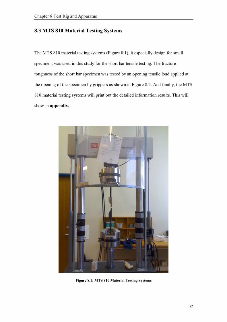
Chapter 8 Test Rig and Apparatus
82
8.3 MTS 810 Material Testing Systems
The MTS 810 material testing systems (Figure 8.1), it especially design for small
specimen, was used in this study for the short bar tensile testing. The fracture
toughness of the short bar specimen was tested by an opening tensile load applied at
the opening of the specimen by grippers as shown in Figure 8.2. And finally, the MTS
810 material testing systems will print out the detailed information results. This will
show in appendix.
Figure 8.1: MTS 810 Material Testing Systems

Chapter 8 Test Rig and Apparatus
83
Figure 8.2: Test rig with specimen in position
High Tensile bolt
Specimen
Grippers
Low Tensile bolt

Chapter 8 Test Rig and Apparatus
84
8.4 The Advantages of MTS 810 Material Testing Systems
Figure 8.3: The systems of MTS 810 Material Testing Systems (MTS 810 FlexTest™
Material Testing Systems)
Here are some of the advantages over then other test rig why MTS 810 machine was
used; its advantages are hereinafter:
# User-friendly: This testing system is incorporated with the TestStart IIs
control system. This system consisted of three major parts: (1) TestStart
system software, (2) digital controller, and (3) remote station control panel as
shown in Figure 8.6.The control system is able to produce the result in the
form of graph or table with the ready programmed software and it also include
some of the important statistical variable such as mean and standard
deviations.

Chapter 8 Test Rig and Apparatus
85
# Accuracy: Its superior axial and lateral stiffness are achieved through an
integral actuator design, stiff, but low mass crosshead, and specially force
transducer.
# Flexibility: By simply changing or adjusting its grips and fixtures. This testing
machine can also be used for many types of testing such as tensile testing,
fatigue life studies, Asphalt or soil testing and etc
8.5 Gripper Design
Due to MTS 810 machine is suitable for tensile testing involving smaller load and can
provides more accurate results, the MTS 810 Material Testing System was used in
this project. Small modification was made to the grippers for enable them to be placed
to the machine. The grippers were hold by high tensile bolts as shown in Figure 8.2.
There are some alternatives to design the grippers as illustrated in the Figure 8.4.
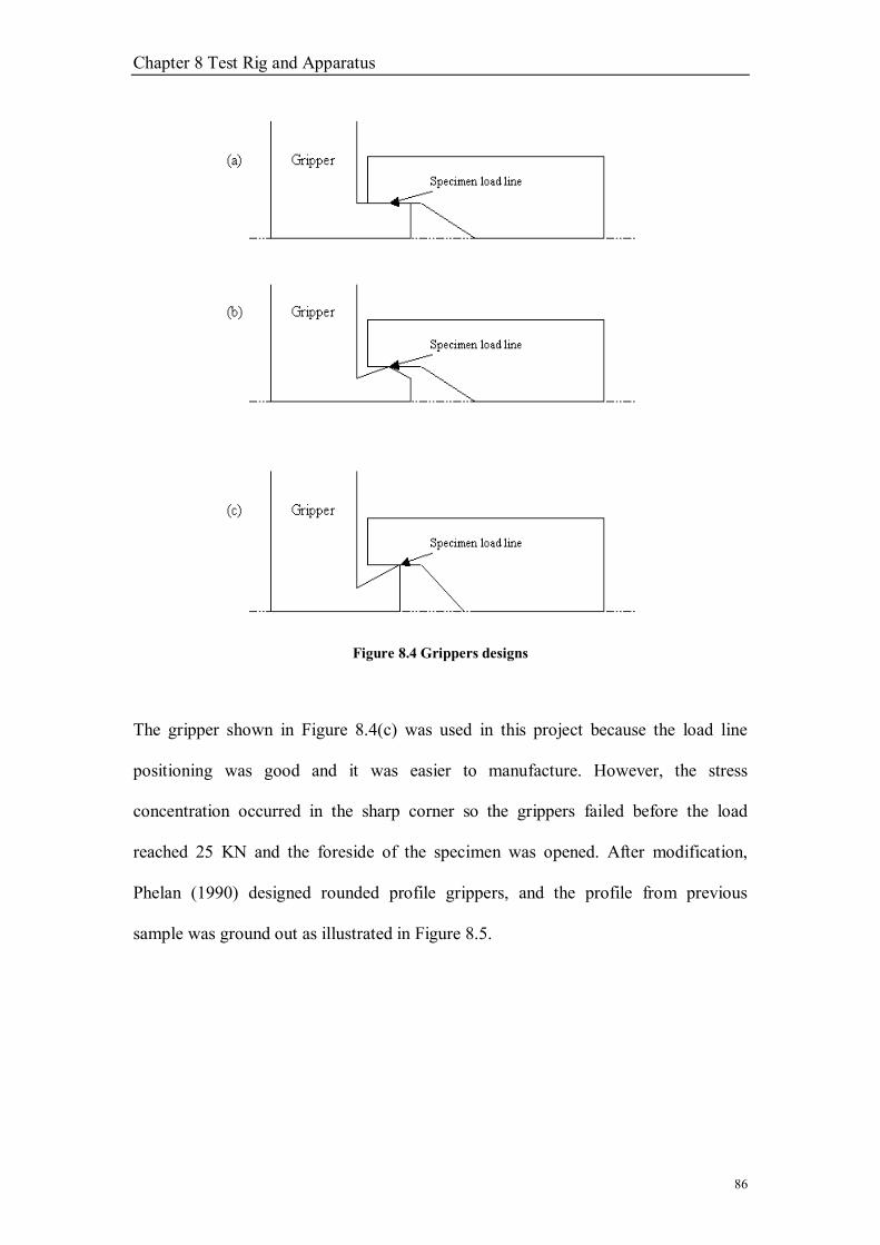
Chapter 8 Test Rig and Apparatus
86
Figure 8.4 Grippers designs
The gripper shown in Figure 8.4(c) was used in this project because the load line
positioning was good and it was easier to manufacture. However, the stress
concentration occurred in the sharp corner so the grippers failed before the load
reached 25 KN and the foreside of the specimen was opened. After modification,
Phelan (1990) designed rounded profile grippers, and the profile from previous
sample was ground out as illustrated in Figure 8.5.

Chapter 8 Test Rig and Apparatus
87
Figure 8.5: The rounded profile of the grippers
Figure 8.6: MTS 810 Material testing System
Rounded corner

Chapter 9 Results and Discussions
88
Chapter 9
Results and Discussions
9.1 Introduction
The results obtained from the experimental work will be present in this chapter. The
chapter will be divided into sections; (1) related to e tensile testing results from the
experimental work, and (2) discuss and determine the fracture toughness; then
compare the results of the fracture toughness and other parameters for VE cured under
different conditions. In the final section, specimens cured in ambient conditions will
be compared with those cured with different microwave conditions having power
levels of 180 Watts, 360 Watts, 540 Watts and 720 Watts.
9.2 MTS-810 tensile testing machine
This MTS 810 tensile testing was used to calculate the fracture toughness. During the
test, a constantly increasing force will apply at the top edge of the specimen until the
load reach maximum and crack occurred. A crack forms at the tip of the notch would
proceed down the specimen along the notched path. By knowing the location of the
crack at the maximum load under linear elastic fracture condition and the height of the
crack that corresponds to the maximum constant load force, the fracture toughness of
the composite can be calculated. Specimens after testing are illustrated in Figure 9.1.

Chapter 9 Results and Discussions
89
Figure 9.1: The fractured specimens and show the part for making the chevron slot
The curing conditions in this project were divided into five major groups. First
condition is cured under ambient conditions for 24 hours; second condition is cured
under 180 Watts microwave conditions, third condition is cured under 360 Watts
microwave conditions, fourth condition is cured under 540 Watts microwave
conditions and fifth condition is cured under 720 Watts microwave conditions For 180
Watts and 360 Watts, exposure times were 60 seconds, 70 seconds and 80 seconds;
with a power of 540 Watts and 720 Watts exposure times were 15 seconds, 20
seconds and 25 seconds. The result obtained by MTS-810 for all curing conditions are
shown in Appendix C. The tensile testing results generated by MTS-810 machine
included the peak load, failure load, break load and the break load elongation of the
specimen. The tensile test result obtained from MTS 810 is illustrated in Figure 9.2.
The three phases listed decide whether the tensile test specimen has been successful
or failed.
Part for making the chevron slot

Chapter 9 Results and Discussions
90
1) The rate of extension was set at 1 mm per minute, which results in the
increased load to initiate the specimen crack
2) The elongation behavior will be show when the specimen passes its peak
load.
3) The crack will be elongated and will reach point 4 of the four critical points
shown in Figure 9.3 and the specimen will show brittle behavior in this area.
In some of the samples, for example the 720 Watts power level with 25 seconds of
exposure time (Figure 9.4), the specimen crack early. This happen, due to the cause of
a bad quality casting when stick the chevron slot. Barker (1980) defined this effect as
crack curve jumping as illustrated in Figure 9.4. Therefore this specimen is not fully
fractured but accruing the crack at the side of it.
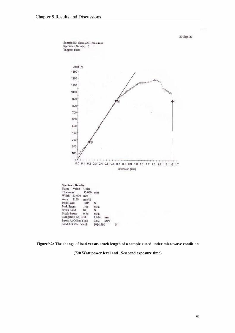
Chapter 9 Results and Discussions
91
Figure9.2: The change of load versus crack length of a sample cured under microwave condition
(720 Watt power level and 15-second exposure time)

Chapter 9 Results and Discussions
92
Figure 9.3: Five critical points for the fractures surface to be analyzed.
Figure 9.4: The change of load versus crack length of a sample cured under microwave condition
(720 Watt power level and 25-second exposure time)

Chapter 9 Results and Discussions
93
9.3 Fracture Toughness Determinations and Discussion
The purpose of the fracture toughness is to determine the severity of a pre-existing
defect in term of its tendency to initiate a fracture. The critical fracture toughness
value KIC was determined with the compact specimens using 5 % secant method. To
determine the fracture toughness (KIC) of a material with the standard test methods,
the K-calibration was made according to the ASTM E399-78.
For the evaluation of K-calibration, K was calculated from the maximum load applied
from the tensile testing and the crack length which is shown as Figure 9.5.
Figure 9.5: Cross-section dimension of short bar specimen

Chapter 9 Results and Discussions
94
9.3.1 The formulas and methods for calculating the fracture
toughness
Specimen cured in 720 Watts with 15 seconds exposure time was taken as an example.
The formulas and methods to obtain the fracture toughness were illustrated as follows:
The formulas used to calculate the fracture toughness were Equations 9.1 through 9.4.
KICSB = WBYF m )( *
max (Eqn. 9.1)
where Fmax = Peak load
Ym* is the compliance calibration according to ASTM E-399-78 standard.
ω = HW =
5.3770 = 1.867 (Eqn. 9.2)
α0 = Wa0 =
7025 = 0.357 (Eqn. 9.3)
α1= Wa1 =
7065 = 0.929 (Eqn. 9.4)
The calculations for it were made by Munz (1981).
Ym* = {- 0.36 + 5.48ω +0.08ω2 + (30.65 - 27.49ω+7.46ω) α0
+ (65.90 + 18.44ω - 9.76ω)α02}
21
0
01
1
−−ααα
Ym*=17.1718

Chapter 9 Results and Discussions
95
The results of the 720-Watt power level and 15-second cured group (six specimens)
were shown in Table 9.1. The mean ( µ ) of fracture toughness is 45.00 N.mm �3/2 .
Peak load Elongation at Break
Break Load
Fracture Toughness
Specimens
(N) (Mm) (N) (N.mm �3/2)
1 1076 1.733 603 44.17 2 1205 1.614 871 49.46 3 1133 2.168 780 46.51 4 1023 1.693 746 41.99 5 1090 1.492 726 44.74 6 1050 1.43 810 43.10
Mean 1096 1.689 756 45.00 Standard Deviation
65 0.262 91 2.44
Table 9.1: Test results of 720 Watts and 15-second exposure
Using KICSB = WBYF m )( *
max (Eqn. 9.5)
and let B = 50 (by design) and W = 70 (not 1.5B);,
From the Table 9.1 mean of Peak Load = Fmax = 1096 N
and Ym =17.1718
therefore KICSB = 7050
)1718.171096( x = 45.00 (N.mm �3/2)

Chapter 9 Results and Discussions
96
9.3.2 Summary Results of Specimens:
There are total thirteen groups of testing in this experiment, those were 180 Watts and
360 Watts with 60 seconds, 70 seconds and 80 seconds exposure time and 540 Watts
and 720 Watts with 15 second, 20 second and 25 second exposure time and the
specimen which cure in ambient condition. Each group has six specimens. For the
mean fracture toughness, we will take the average of all six specimens in the same
group. So we can examine that the mean of fracture toughness is become around 42
N.mm �3/2 to 48 N.mm �3/2 . The results as shown as below from Table 9.2 � Table
9.14
1. Test results in ambient conditions
Table 9.2: Test results of ambient condition
Peak load
Elongation at Break
Break Load
Fracture Toughness
Specimens
(N) (Mm) (N) (N.mm �3/2)
1 1033 1.966 739 42.40 2 1036 2.348 908 42.53 3 1071 2.185 819 43.96 4 1075 1.766 657 44.13 5 1056 1.799 841 43.35 6 1012 1.806 622 41.54
Mean 1047 1.978 764 42.98 Standard Deviation
24 0.239 111 0.92

Chapter 9 Results and Discussions
97
2. Test results of 180 Watts with 60 seconds
Table 9.3: Test results of 180 Watts with 60 seconds
Peak load
Elongation at Break
Break Load
Fracture Toughness
Specimens
(N) (Mm) (N) (N.mm �3/2)
1 1074 1.483 952 44.09 2 1028 1.596 748 42.20 3 982 1.351 879 40.31 4 1044 1.847 779 42.85 5 1125 1.934 757 46.18 6 1071 1.902 795 43.96
Mean 1054 1.685 818 43.27 Standard Deviation
48 0.243 81 1.81
3. Test results of 180 Watts with 70 seconds
Table 9.4: Test results of 180 Watts with 70 seconds
Peak load
Elongation at Break
Break Load
Fracture Toughness
Specimens
(N) (Mm) (N) (N.mm �3/2)
1 1126 1.57 662 46.22 2 1120 1.429 783 45.97 3 1159 1.956 1045 47.58 4 1124 1.624 1017 46.14 5 1124 1.822 773 46.14 6 1143 1.637 824 46.92
Mean 1133 1.673 851 46.49 Standard Deviation
15 0.188 150 0.57

Chapter 9 Results and Discussions
98
4. Test results of 180 Watts with 80 seconds
Table 9.5: Test results of 180 Watts with 80 seconds
Peak load
Elongation at Break
Break Load
Fracture Toughness
Specimens
(N) (Mm) (N) (N.mm �3/2)
1 1196 1.536 1118 49.09 2 1080 1.749 953 44.33 3 1162 1.954 875 47.70 4 1040 1.791 764 42.69 5 1067 1.668 628 43.80 6 1069 2.073 551 43.88
Mean 1102 1.795 815 45.25 Standard Deviation
61 0.194 211 2.31
5. Test results of 360 Watt power with 60 seconds
Table 9.6: Test results of 360 Watts with 60 seconds
Peak load
Elongation at Break
Break Load
Fracture Toughness
Specimens
(N) (Mm) (N) (N.mm �3/2)
1 1191 1.627 868 48.89 2 1093 1.645 845 44.87 3 1293 1.966 1138 53.08 4 1126 1.92 986 46.22 5 1159 2.136 1068 47.58 6 1102 2.147 842 45.24
Mean 1161 1.907 958 47.64 Standard
Deviation
74 0.228 126 2.79

Chapter 9 Results and Discussions
99
6. Test results of 360 Watt power with 70 seconds
Table 9.7: Test results of 360 Watts with 70 seconds
Peak load
Elongation at Break
Break Load
Fracture Toughness
Specimens
(N) (Mm) (N) (N.mm �3/2)
1 1111 1.977 992 45.60 2 1081 1.712 971 44.37 3 1098 1.747 626 45.07 4 1014 1.674 786 41.62 5 1088 2.234 747 44.66 6 1097 2.059 942 45.03
Mean 1082 1.9 844 44.39 Standard Deviation
35 0.225 147 1.30
7. Test results of 360 Watt power with 80 seconds
Table 9.8: Test results of 360 Watts with 80 seconds
Peak load
Elongation at Break
Break Load
Fracture Toughness
Specimens
(N) (Mm) (N) (N.mm �3/2)
1 1079 1.985 928 44.29 2 1042 1.852 796 42.77 3 1020 2.126 787 41.87 4 1046 2.041 826 42.94 5 1141 1.949 963 46.84 6 1024 1.965 908 42.03
Mean 1059 1.986 868 43.46 Standard
Deviation
45 0.092 74 1.70

Chapter 9 Results and Discussions
100
8. Test results of 540 Watt power with 15 seconds
Table 9.9: Test results of 540 Watts with 15 seconds
Peak load
Elongation at Break
Break Load
Fracture Toughness
Specimens
(N) (Mm) (N) (N.mm �3/2)
1 1215 1.4 1194 49.87 2 1080 1.515 771 44.33 3 990 1.498 601 40.64 4 1061 1.926 892 43.55 5 1097 1.544 874 45.03
Mean 1089 1.576 866 44.69 Standard Deviation
82 0.202 216 2.99
9. Test results of 540 Watt power with 20 seconds
Table 9.10: Test results of 540 Watts with 20 seconds
Peak load
Elongation at Break
Break Load
Fracture Toughness
Specimens
(N) (Mm) (N) (N.mm �3/2)
1 1111 1.502 765 45.60 2 1053 1.783 801 43.22 3 1060 1.669 916 43.51 4 1212 1.843 830 49.75 5 1164 1.78 989 47.78 6 1182 1.962 898 48.52
Mean 1130 1.756 866 46.40 Standard Deviation
66 0.157 83 2.47

Chapter 9 Results and Discussions
101
10. Test results of 540 Watt power with 25 seconds
Table 9.11: Test results of 540 Watts with 25 seconds
Peak load
Elongation at Break
Break Load
Fracture Toughness
Specimens
(N) (Mm) (N) (N.mm �3/2)
1 1100 1.919 692 45.15 2 1023 1.506 566 41.99 3 1020 1.515 659 41.87 4 1039 1.5 727 42.65 5 1091 1.521 730 44.78 6 1121 1.767 1024 46.02
Mean 1066 1.621 733 43.74 Standard Deviation
43 0.178 155 1.63
11. Test results of 720 Watt power with 15 seconds
Table 9.12: Test results of 720 Watts with 15 seconds
Peak load
Elongation at Break
Break Load
Fracture Toughness
Specimens
(N) (Mm) (N) (N.mm �3/2)
1 1076 1.733 603 44.17 2 1205 1.614 871 49.46 3 1133 2.168 780 46.51 4 1023 1.693 746 41.99 5 1090 1.492 726 44.74 6 1050 1.43 810 43.10
Mean 1096 1.689 756 45.00 Standard
Deviation
65 0.262 91 2.44

Chapter 9 Results and Discussions
102
12. Test results of 720 Watt power with 20 seconds
Table 9.13: Test results of 720 Watts with 20 seconds
Peak load
Elongation at Break
Break Load
Fracture Toughness
Specimens
(N) (Mm) (N) (N.mm �3/2)
1 1111 1.833 989 45.60 2 1100 1.76 1005 45.15 3 1173 1.926 1044 48.15 4 1104 1.94 329 45.32 5 1128 1.98 1003 46.30 6 1124 1.793 1077 46.14
Mean 1123 1.872 908 46.11 Standard Deviation
27 0.089 285 1.00
13. Test results of 720 Watt power with 25 seconds
Table 9.14: Test results of 720 Watts with 25 seconds
Peak load
Elongation at Break
Break Load
Fracture Toughness
Specimens
(N) (Mm) (N) (N.mm �3/2)
1 1125 2.014 1052 46.18 2 1145 0.905 1145 47.00 3 1043 1.669 617 42.81 4 1077 1.699 763 44.21 5 1103 1.588 671 45.28 6 1153 1.589 927 47.33
Mean 1108 1.577 863 45.47 Standard Deviation
42 0.365 213 1.58

Chapter 9 Results and Discussions
103
The summary of fracture toughness values of the composites cured under different
conditions are summarized in Table 9.15. The values of fracture toughness of samples
cured under ambient conditions, 42.9846 N.mm �3/2 were converted to 100 % for ease
of comparison; other values were also similarly converted to percentage using
42.9846 N.mm �3/2 as base.

Cha
pter
9 R
esul
ts a
nd D
iscus
sions
10
4
T
able
9.1
5: R
esul
t of t
he fr
actu
re to
ughn
ess a
nd o
ther
par
amet
ers f
or V
E/F
LY
ASH
(33%
) cur
ed u
nder
diff
eren
t co
nditi
on
Con
ditio
n Am
bien
t 18
0 W
att
360
Wat
t 54
0 W
att
720
Wat
t
Tim
e N
il 60
s 70
s 80
s 60
s 70
s 80
s 15
s 20
s 25
s 15
s 20
s 25
s
Elon
gatio
n At
Bre
ak
(mm
) 1.
978
1.68
5 1.
673
1.79
5 1.
907
1.9
1.98
6 1.
576
1.75
6 1.
621
1.68
9 1.
872
1.57
7
Peak
Loa
d (N
) 10
47
1054
11
33
1102
11
61
1082
10
59
1089
11
30
1066
10
96
1123
11
08
Bre
ak L
oad
(N)
764
818
851
815
958
844
868
866
866
733
756
908
863
Frac
ture
To
ughn
ess
( N.m
m �3
/2)
42.9
846
43
.265
1 4
6.49
43
45.2
491
47.6
436
44.3
939
43.4
567
44.
6854
46
.398
5 43
.744
0 44
.996
0 46
.111
1 45
.468
1
Rel
ativ
e fr
actu
re
toug
hnes
s 10
0%
101%
10
8%
105%
11
1%
103%
10
1%
104%
10
8%
102%
10
5%
107%
10
6%
Stan
dard
D
evia
tion
0.92
1.
81
0.57
2.
31
2.79
1.
30
1.70
2.
99
2.47
1.
63
2.44
1.
00
1.58

Chapter 9 Results and Discussions
105
From Table 9.15, we can found that the fracture toughness of the sample treated with
180 Watts with exposures time of 60, 70 and 80 seconds is higher than that of the
ambient cured samples from 1- 8 %; With microwave parameters of 360 Watts with
exposures time of 60 � 80 seconds, specimens cured under microwave are higher than
specimen which cured under ambient condition from 1 - 11%. With microwave
parameters of 540 Watts and shorter duration of exposures of 15, 20 and 25 seconds,
the fracture toughness is higher than those cured under ambient conditions from 2 � 8
%; for 720 Watts and same exposures time of 15, 20 and 25 seconds, the fracture
toughness is higher than those cured under ambient conditions from 5 � 7 %.
All values of fracture toughness of VE/FLYASH (33%) cured under microwave
conditions are within or above 5 percent upper marker of those cured under ambient
conditions. This means microwave irradiation reduces the shrinkage of the composite
but at the same time improves its fracture toughness. The results are shows in Figure
9.6 and Figure 9.7.
The results have been published by Dr. Harry Ku be entitled �An Evaluation if
Fracture Toughness of Vinyl Ester Composites Cured Under Microwave Condition�
in Journal of Materials Engineering and Performance.

Chapter 9 Results and Discussions
106
Fracture toughness of VE/FLY ASH (33%)
92
96
100
104
108
112
50 60 70 80 90
Duration of exposure to microwaves
Rel
ativ
e fr
actu
re
toug
hnes
sAmbient180 W
360 W
Figure 9.6: Fracture toughness of VE/FLYASH (33%) cured under 180 Watts and 360 Watts of
microwave power
Fracture toughness of VE/FLY ASH (33%)
96
100
104
108
112
10 15 20 25 30
Duration of exposure to microwaves
Rel
ativ
e fr
actu
reto
ughn
ess
Ambient
540 W
720 W
Figure 9.7: Fracture toughness of VE/FLYASH (33%) cured under 540 Watts and 720 Watts of
microwave power

Chapter 10 Conclusion and Recommendations
107
Chapter 10
Conclusion and Recommendations
10.1 Conclusion
In this study, the fracture toughness values obtained are higher than those obtained by
previous study. In general, the higher fracture toughness values obtained in this
study is might because of the better material used to make the mould and
improvement in design. In previous study, cardboard was used to make the moulds
and this allows the resin to penetrate into the cardboard and seep through the gaps
between the adjoining areas of the cardboard; the resulting composite would then
have a higher percentage by weight of fly ash and hence they are less tough. When
the samples were cured under microwave conditions, the situation became worse as
the initial expansion of the composite due to microwave irradiation forced more resin
to penetrate into the cardboard and seep through the adjoining gaps. However in this
study, this did not happen as the moulds were made of plastic, which may deform
after several microwave processing and a new mould has to be machined.
However, all the study prove that the exposure of the samples by microwave irradiation
did reduce the shrinkage of the vinyl ester composite but at the same time the toughness
of the material was retained. Provided a suitable combination of power level and
duration of exposure were selected in the treatment. For those higher power levels like
540 Watts and 720 Watts, much shorter duration of exposure is required.
Chapter 10 Conclusion and Recommendations
108
10.2 Recommendations
The results can be improved throughout the following efforts:
• Changing a new mould after several testing to prevent the deformation of
mould after several microwave processing. Maintain the specimen size to get
more accurate results.
• Improve material properties of the triangle mould which and recyclable use
and structure of specimen: By using a better material especially the chevron
slot part should be made of harder material so that the part would not be bend
aside.
• Use Latin Square to analyse the result and fractured surface analysis using
SEM (Scanning Electron Microscope), in which five critical points of the
fractured surface to be analyzed. The surface of chevron cut may deteriorated
by scratching or compressing it with the other materials. These actions might
damage the important features of the crack on the chevron surface, thus the
specimens are suggested to keep in a solid container and they should be taken
for SEM testing as soon as possible after the tensile testing.
• Simulation by analysing software: More information can be obtained if
computer software is used to analyse the experimental results, example like
the area of maximum fracture toughness and etc. Suggest using the software

Chapter 10 Conclusion and Recommendations
109
package called ANSYS, because it is user-friendly and it can be incorporated
with other software such as PRO-ENGINEER and so on.

References
110
References
Ang, S F, 2004, Evaluation Impact Strength on Particulate Reinforced (25% and 33%)
Vinyl Ester Composite Cured Under Microwave Conditions
Askeland, D R, 1998, The Science and Engineering of Materials, 3rd edn, Stanley
Thornes.
Astrom, B T 1997, Manufacturing of Polymer Composites, Chapman and Hall, United
Kingdom
Baddeley, D T and Ballard J, 1991, Evaluate the Short Rod/Bar Fracture Mechanics
Test, BEng Thesis of Jennine Ballard, School of Mechanical and Manufacturing
Engineering, Queensland University of Technology, Australia.
Brady, G. S. & Clauser, H. R. 1991, Material Handbook, 13th edn, McGraw-Hill Inc.,
New York.
Barker, L M, 1979, Fracture Mechanics Applied to Brittle Materials, ASTM, STP
678, American Society for Testing and Materials.
Baker, L M, 1980, Development of the Short Road Method of Fracture Toughness
Measurement, Proceedings, Conference on Wear and Fracture Prevention, 21-22
May 1980, ASM, Metals Park, Ohio, pp. 163-180.

References
111
Baker, L M, 1981, Short Rod and Short Bar Fracture Toughness Specimen
Geometries and Test Methods for Metallic Materials, Proceedings, Fracture
Mechanics: Thirteenth Conference, ASMT STP 743, 1981, pp. 456-475.
Bolton, W, 1996, Materials and Their Uses, Butterworth and Heinemann, p. 128.
Callister, W D, 2003, Materials Science and Engineering: An Introduction, 6th edn,
John Wiley and Sons, Inc., pp. 201-203.
Clarke, J L Editor, 1996, Structural design of polymer composites, E & FN Spon,
United Kingdom.
Denes, J and Keedwell, A D, 1974, Latin Squares and their Applications, English
University Press Ltd., pp.1-41.
J. Thuery, 1992, Microwaves Industrial, Scientific and Medical Applications, Artech
House, Inc., United Kingdom.
Kalpakjian, S. 1991, Manufacturing Processes for Engineering Materials, 2nd edn,
Addison-Wesley Publishing Company.
Ku, H S, Siores, E, Ball, J A R and Horsfield, B (1999a), Microwave Processing and
Permittivity Measurement of Thermoplastic Composites at Elevated Temperatures,

References
112
Journal of Materials Processing Technology, United States of America, Vol. 89-90, pp.
419-24.
Ku, H S, Siores, E, Ball, J A R (1999b), Microwave Facilities for Welding
Thermoplastic Composites, and Preliminary Results, Journal of Microwave Power
and Electromagnetic Energy, United States of America, Vol. 34, No. 4, pp. 195-205.
Ku, H S, Siores, E, Ball, J A R and Horsfiled, B (2001), Permittivity Measurement of
Thermoplastic Composites at Elevated Temperature, Journal of Microwave Power
and Electromagnetic Energy, United States of America, Vol. 36, No. 2, pp. 101-111.
Ku, H S, Van Erp, G, Ball, J A R and Ayers, S (2002a), Shrinkage Reduction of
Thermoset Fibre Composites during Hardening using Microwaves Irradiation for
Curing, Proceedings, Second World Engineering Congress, Kuching, Malaysia, 22-25
July, pp. 177-182.
Ku, H S (2002b), Risks involved in curing vinyl ester resins using microwaves
irradiation, Journal of Material Synthesis and Processing, Vol. 10, No. 2, pp. 97 -106.
Lubin, G. (ed.) 1982, Handbook of Composites, Van Nostrand Reinhold, New York.
Mallick, P.K. (ed.) 1997, Composite Engineering Handbook, Marcel Dekker, Inc.

References
113
Matthews, F L and Rawlings, R.D, 1994, Composite Materials: Engineering and
Science, 1st edn, Chapman and Hall, United Kingdom.
Metaxas, A C. and Meredith, R J, 1983, Industrial Microwave Heating, Peter
Peregrinus Ltd., pp. 5-6, 28-31, 43, 211, 217, 278, 284-5.
Munz, D, 1981, Determination of Fracture Toughness of High Strength Aluminum
Alloys with Cheron Notched Short Rod and Short Bar Specimens, Engineering
Fracture Mechanics, Vol. 15, No. 1-2, pp. 231-236.
Murdoch, J and Barnes, J A, 1975, Statistical Tables for Science, Engineering and
Management, Macmillan, p.9.
Tsang, S H, 2002, Fracture Analysis of Vinyl Ester Composites Under Microwave
Condition
(NRC) National Research Council, 1994, Microwave Processing of Materials,
National Materials Advisory Board, Commission on Engineering and Technical
Systems, National Academy Press, United States of America.
Okine, R.K. (ed.) 1997, Composite Engineering Handbook, Marcel Dekker, Inc.
Osswald, T A and Menges, G, 1995, Materials Science of Polymers for Engineers,
Hanser Publishers, New York.

References
114
Peters, S T, 1998, Handbook of Composites, Chapman and Hall, United Kingdom.
Pritchard, G, 1999, Reinforced Pastics Drability, Woodhead publishing Ltd., United
Kingdom.

Appendix
a
Appendix A
Project Specification

Appendix
b
University of Southern Queensland
Faculty of Engineering and Surveying
ENG 4111 Research Project Part 2
PROJECT SPECIFICATION
Project Title : Fracture Analysis of Vinyl Ester Composite Cured under
Microwave Condition
Student Name : Mr. Wooi Lieh, CHAN
Student Number : 0050027343
Supervisor : Dr. Harry Ku
Project Synopsis:
This project is to find out the fracture toughness of particulate reinforced vinyl ester
resins cured microwave conditions. Short bar method will be used. SEM will also be
used to analyze the fracture mechanics of the composites cured under ambient
conditions. The percentages by weight of the fly ash (reinforcement) are 25% and
33%. The data collected may be useful in supporting the development of FCDD group
in future.
Timelines of Specific Activities:
1. Familiarization of equipment and literature reviews.
Begin : 6th March 2006
Completion : 16th April 2006
Approx. Hours : 55 hours
2. Make samples of Vinyl Ester for testing using microwave and at ambient
condition.
Begin : 17th April 2006
Completion : 26th May 2006
Approx. Hours : 60 hours
3. Analysis of results and compare other variables.
Begin : 29th May 2006
Completion : 31st July 2006

Appendix
c
Approx. Hours : 55 hours
4. Draw up conclusion.
Begin : 1st August 2006
Completion : 2nd September 2006
Approx. Hours : 30 hours
5. Thesis outline � to be discussed with supervisor.
Begin : 4th September 2006
Completion : 11th September 2006
Approx. Hours : 10 hours
6. Thesis first draft � each chapter to be shown to supervisor
Begin : 12th September 2006
Completion : 12th October 2006
Approx. Hours : 60 hours
7. Final draft of thesis, to incorporate modifications suggest by supervisor.
Begin : 13th October 2006
Completion : 2nd November 2006
Approx. Hours : 30 hours
AGREED: __________________ (student) __________________ (Supervisors)
(date)___/___/___

Appendix
d
Appendix B
Auto-CAD drawing

Appendix
e
The Auto-CAD drawing for the triangle part of the mould

Appendix
f
Dimension of Short Bar using in Testing

Appendix
g
Appendix C
Testing Results Obtained from
MTS-810 of all Conditions

Appendix
h
Chan-ambient Test Date : 20-Sep-06 Method : MMT fracture toughness Test .msm Specimen Results: Specimen
# Thickness
mm Width
mm Area
mm^2 Peak Load
N Peak Stress MPa
Break Load
N
Break Stress MPa
1 50.000 23.000 1150 1033 0.90 739 0.64 2 50.000 23.000 1150 1036 0.90 908 0.79 3 50.000 23.000 1150 1071 0.93 819 0.71 4 50.000 23.000 1150 1075 0.94 657 0.57 5 50.000 23.000 1150 1056 0.92 841 0.73 6 50.000 23.000 1150 1012 0.88 622 0.54 Mean 50.000 23.000 1150 1047 0.91 764 0.66 Std Dev 0.000 0.000 0 24 0.02 111 0.10 Specimen
# Elongation At Break
mm
Stress At Offset Yield MPa
Load At Offset Yield
N
1 1.966 0.744 856.158 2 2.348 0.818 941.296 3 2.185 0.794 912.636 4 1.766 0.841 966.754 5 1.799 0.786 903.364 6 1.806 0.742 852.786 Mean 1.978 0.787 905.499 Std Dev 0.239 0.039 45.392
0
100
200
300
400
500
600
700
800
900
1000
1100
0.0 0.2 0.4 0.6 0.8 1.0 1.2 1.4 1.6 1.8 2.0 2.2 2.4
Load (N)
Extension (mm)

Appendix
i
Chan-180-60n Test Date : 20-Sep-06 Method : MMT fracture toughness Test .msm Specimen Results:
Specimen
#
Thickness mm
Width mm
Area mm^2
Peak Load N
Peak Stress MPa
Break Load
N
Break Stress MPa
1 50.000 23.000 1150 1074 0.93 952 0.83 2 50.000 23.000 1150 1028 0.89 748 0.65 3 50.000 23.000 1150 982 0.85 879 0.76 4 50.000 23.000 1150 1044 0.91 779 0.68 5 50.000 23.000 1150 1125 0.98 757 0.66 6 50.000 23.000 1150 1071 0.93 795 0.69 Mean 50.000 23.000 1150 1054 0.92 818 0.71 Std Dev 0.000 0.000 0 48 0.04 81 0.07 Specimen
# Elongation At Break
mm
Stress At Offset Yield MPa
Load At Offset Yield
N
1 1.483 0.780 897.294 2 1.596 0.874 1005.192 3 1.351 0.788 906.735 4 1.847 0.791 910.107 5 1.934 0.843 969.957 6 1.902 0.798 918.200 Mean 1.685 0.813 934.581 Std Dev 0.243 0.037 43.059
0
100
200
300
400
500
600
700
800
900
1000
1100
1200
0.0 0.1 0.2 0.3 0.4 0.5 0.6 0.7 0.8 0.9 1.0 1.1 1.2 1.3 1.4 1.5 1.6 1.7 1.8 1.9 2.0
Load (N)
Extension (mm)

Appendix
j
Chan-180-70n Test Date : 31-Aug-06 Method : MMT fracture toughness Test .msm Specimen Results:
Specimen
#
Thickness mm
Width mm
Area mm^2
Peak Load N
Peak Stress MPa
Break Load
N
Break Stress MPa
1 23.000 50.000 1150 1126 0.98 662 0.58 2 23.000 50.000 1150 1120 0.97 783 0.68 3 23.000 50.000 1150 1159 1.01 1045 0.91 4 23.000 50.000 1150 1124 0.98 1017 0.88 5 23.000 50.000 1150 1124 0.98 773 0.67 6 23.000 50.000 1150 1143 0.99 824 0.72 Mean 23.000 50.000 1150 1133 0.98 851 0.74 Std Dev 0.000 0.000 0 15 0.01 150 0.13 Specimen
# Elongation At Break
mm
Stress At Offset Yield MPa
Load At Offset Yield
N
1 1.570 0.853 981.456 2 1.429 0.888 1021.244 3 1.956 0.938 1078.565 4 1.624 0.969 1114.643 5 1.822 0.907 1042.824 6 1.637 0.906 1041.475 Mean 1.673 0.910 1046.701 Std Dev 0.188 0.040 45.997
0
100
200
300
400
500
600
700
800
900
1000
1100
1200
0.0 0.1 0.2 0.3 0.4 0.5 0.6 0.7 0.8 0.9 1.0 1.1 1.2 1.3 1.4 1.5 1.6 1.7 1.8 1.9 2.0
Load (N)
Extension (mm)
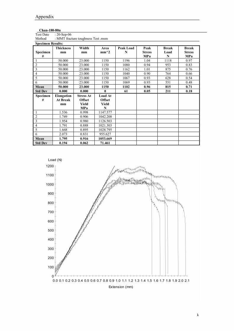
Appendix
k
Chan-180-80n Test Date : 20-Sep-06 Method : MMT fracture toughness Test .msm Specimen Results:
Specimen
#
Thickness mm
Width mm
Area mm^2
Peak Load N
Peak Stress MPa
Break Load
N
Break Stress MPa
1 50.000 23.000 1150 1196 1.04 1118 0.97 2 50.000 23.000 1150 1080 0.94 953 0.83 3 50.000 23.000 1150 1162 1.01 875 0.76 4 50.000 23.000 1150 1040 0.90 764 0.66 5 50.000 23.000 1150 1067 0.93 628 0.54 6 50.000 23.000 1150 1069 0.93 551 0.48 Mean 50.000 23.000 1150 1102 0.96 815 0.71 Std Dev 0.000 0.000 0 61 0.05 211 0.18 Specimen
# Elongation At Break
mm
Stress At Offset Yield MPa
Load At Offset Yield
N
1 1.536 0.998 1147.577 2 1.749 0.906 1042.208 3 1.954 0.980 1126.503 4 1.791 0.888 1021.303 5 1.668 0.895 1028.795 6 2.073 0.831 955.627 Mean 1.795 0.916 1053.669 Std Dev 0.194 0.062 71.461
0
100
200
300
400
500
600
700
800
900
1000
1100
1200
0.0 0.1 0.2 0.3 0.4 0.5 0.6 0.7 0.8 0.9 1.0 1.1 1.2 1.3 1.4 1.5 1.6 1.7 1.8 1.9 2.0 2.1
Load (N)
Extension (mm)

Appendix
l
Chan-360-60n Test Date : 20-Sep-06 Method : MMT fracture toughness Test .msm Specimen Results:
Specimen
#
Thickness mm
Width mm
Area mm^2
Peak Load N
Peak Stress MPa
Break Load
N
Break Stress MPa
1 50.000 23.000 1150 1191 1.04 868 0.75 2 50.000 23.000 1150 1093 0.95 845 0.73 3 50.000 23.000 1150 1293 1.12 1138 0.99 4 50.000 23.000 1150 1126 0.98 986 0.86 5 50.000 23.000 1150 1159 1.01 1068 0.93 6 50.000 23.000 1150 1102 0.96 842 0.73 Mean 50.000 23.000 1150 1161 1.01 958 0.83 Std Dev 0.000 0.000 0 74 0.06 126 0.11 Specimen
# Elongation At Break
mm
Stress At Offset Yield MPa
Load At Offset Yield
N
1 1.627 0.972 1118.316 2 1.645 0.932 1071.954 3 1.966 0.948 1089.993 4 1.920 0.878 1009.913 5 2.136 0.907 1043.462 6 2.147 0.849 976.195 Mean 1.907 0.914 1051.639 Std Dev 0.228 0.046 52.592
0
100
200
300
400
500
600
700
800
900
1000
1100
1200
1300
0.0 0.2 0.4 0.6 0.8 1.0 1.2 1.4 1.6 1.8 2.0 2.2
Load (N)
Extension (mm)

Appendix
m
Chan-360-70n Test Date : 31-Aug-06 Method : MMT fracture toughness Test .msm Specimen Results:
Specimen
#
Thickness mm
Width mm
Area mm^2
Peak Load N
Peak Stress MPa
Break Load
N
Break Stress MPa
1 23.000 50.000 1150 1111 0.97 992 0.86 2 23.000 50.000 1150 1081 0.94 971 0.84 3 23.000 50.000 1150 1098 0.95 626 0.54 4 23.000 50.000 1150 1014 0.88 786 0.68 5 23.000 50.000 1150 1088 0.95 747 0.65 6 23.000 50.000 1150 1097 0.95 942 0.82 Mean 23.000 50.000 1150 1082 0.94 844 0.73 Std Dev 0.000 0.000 0 35 0.03 147 0.13 Specimen
# Elongation At Break
mm
Stress At Offset Yield MPa
Load At Offset Yield
N
1 1.977 0.859 987.534 2 1.712 0.892 1025.973 3 1.747 0.894 1028.091 4 1.674 0.849 976.671 5 2.234 0.860 988.809 6 2.059 0.813 934.692 Mean 1.900 0.861 990.295 Std Dev 0.225 0.030 34.608
0
100
200
300
400
500
600
700
800
900
1000
1100
1200
0.0 0.2 0.4 0.6 0.8 1.0 1.2 1.4 1.6 1.8 2.0 2.2 2.4
Load (N)
Extension (mm)

Appendix
n
Chan-360-80n Test Date : 20-Sep-06 Method : MMT fracture toughness Test .msm Specimen Results:
Specimen
#
Thickness mm
Width mm
Area mm^2
Peak Load N
Peak Stress MPa
Break Load
N
Break Stress MPa
1 50.000 23.000 1150 1079 0.94 928 0.81 2 50.000 23.000 1150 1042 0.91 796 0.69 3 50.000 23.000 1150 1020 0.89 787 0.68 4 50.000 23.000 1150 1046 0.91 826 0.72 5 50.000 23.000 1150 1141 0.99 963 0.84 6 50.000 23.000 1150 1024 0.89 908 0.79 Mean 50.000 23.000 1150 1059 0.92 868 0.75 Std Dev 0.000 0.000 0 45 0.04 74 0.06 Specimen
# Elongation At Break
mm
Stress At Offset Yield MPa
Load At Offset Yield
N
1 1.985 0.788 906.735 2 1.852 0.873 1003.843 3 2.126 0.825 948.883 4 2.041 0.843 969.114 5 1.949 0.936 1076.337 6 1.965 0.733 843.514 Mean 1.986 0.833 958.071 Std Dev 0.092 0.070 80.059
0
100
200
300
400
500
600
700
800
900
1000
1100
1200
0.0 0.2 0.4 0.6 0.8 1.0 1.2 1.4 1.6 1.8 2.0 2.2
Load (N)
Extension (mm)

Appendix
o
Chan-520-15n Test Date : 20-Sep-06 Method : MMT fracture toughness Test .msm Specimen Results:
Specimen
#
Thickness mm
Width mm
Area mm^2
Peak Load N
Peak Stress MPa
Break Load
N
Break Stress MPa
1 50.000 23.000 1150 1215 1.06 1194 1.04 2 50.000 23.000 1150 1080 0.94 771 0.67 3 50.000 23.000 1150 990 0.86 601 0.52 4 50.000 23.000 1150 1061 0.92 892 0.78 5 50.000 23.000 1150 1097 0.95 874 0.76 Mean 50.000 23.000 1150 1089 0.95 866 0.75 Std Dev 0.000 0.000 0 82 0.07 216 0.19 Specimen
# Elongation At Break
mm
Stress At Offset Yield MPa
Load At Offset Yield
N
1 1.400 0.943 1084.864 2 1.515 0.910 1046.931 3 1.498 0.830 954.881 4 1.926 0.842 968.031 5 1.544 0.878 1009.673 Mean 1.576 0.881 1012.876 Std Dev 0.202 0.047 54.145
0
100
200
300
400
500
600
700
800
900
1000
1100
1200
1300
0.0 0.1 0.2 0.3 0.4 0.5 0.6 0.7 0.8 0.9 1.0 1.1 1.2 1.3 1.4 1.5 1.6 1.7 1.8 1.9 2.0
Load (N)
Extension (mm)

Appendix
p
Chan-540-20n Test Date : 20-Sep-06 Method : MMT fracture toughness Test .msm Specimen Results:
Specimen
#
Thickness mm
Width mm
Area mm^2
Peak Load N
Peak Stress MPa
Break Load
N
Break Stress MPa
1 50.000 23.000 1150 1111 0.97 765 0.66 2 50.000 23.000 1150 1053 0.92 801 0.70 3 50.000 23.000 1150 1060 0.92 916 0.80 4 50.000 23.000 1150 1212 1.05 830 0.72 5 50.000 23.000 1150 1164 1.01 989 0.86 6 50.000 23.000 1150 1182 1.03 898 0.78 Mean 50.000 23.000 1150 1130 0.98 866 0.75 Std Dev 0.000 0.000 0 66 0.06 83 0.07 Specimen
# Elongation At Break
mm
Stress At Offset Yield MPa
Load At Offset Yield
N
1 1.502 0.910 1046.931 2 1.783 0.865 994.668 3 1.669 0.857 985.396 4 1.843 0.945 1087.056 5 1.780 0.941 1082.335 6 1.962 0.891 1025.014 Mean 1.756 0.902 1036.900 Std Dev 0.157 0.037 43.030
0
100
200
300
400
500
600
700
800
900
1000
1100
1200
1300
0.0 0.1 0.2 0.3 0.4 0.5 0.6 0.7 0.8 0.9 1.0 1.1 1.2 1.3 1.4 1.5 1.6 1.7 1.8 1.9 2.0
Load (N)
Extension (mm)

Appendix
q
Chan-540-25n Test Date : 20-Sep-06 Method : MMT fracture toughness Test .msm Specimen Results:
Specimen
#
Thickness mm
Width mm
Area mm^2
Peak Load N
Peak Stress MPa
Break Load
N
Break Stress MPa
1 50.000 23.000 1150 1100 0.96 692 0.60 2 50.000 23.000 1150 1023 0.89 566 0.49 3 50.000 23.000 1150 1020 0.89 659 0.57 4 50.000 23.000 1150 1039 0.90 727 0.63 5 50.000 23.000 1150 1091 0.95 730 0.63 6 50.000 23.000 1150 1121 0.97 1024 0.89 Mean 50.000 23.000 1150 1066 0.93 733 0.64 Std Dev 0.000 0.000 0 43 0.04 155 0.13 Specimen
# Elongation At Break
mm
Stress At Offset Yield MPa
Load At Offset Yield
N
1 1.919 0.834 959.264 2 1.506 0.844 971.066 3 1.515 0.825 948.812 4 1.500 0.857 985.902 5 1.521 0.891 1024.677 6 1.767 0.895 1028.892 Mean 1.621 0.858 986.435 Std Dev 0.178 0.029 33.631
0
100
200
300
400
500
600
700
800
900
1000
1100
1200
0.0 0.1 0.2 0.3 0.4 0.5 0.6 0.7 0.8 0.9 1.0 1.1 1.2 1.3 1.4 1.5 1.6 1.7 1.8 1.9 2.0
Load (N)
Extension (mm)

Appendix
r
Chan-720-15n Test Date : 20-Sep-06 Method : MMT fracture toughness Test .msm Specimen Results:
Specimen
#
Thickness mm
Width mm
Area mm^2
Peak Load N
Peak Stress MPa
Break Load
N
Break Stress MPa
1 50.000 23.000 1150 1076 0.94 603 0.52 2 50.000 23.000 1150 1205 1.05 871 0.76 3 50.000 23.000 1150 1133 0.98 780 0.68 4 50.000 23.000 1150 1023 0.89 746 0.65 5 50.000 23.000 1150 1090 0.95 726 0.63 6 50.000 23.000 1150 1050 0.91 810 0.70 Mean 50.000 23.000 1150 1096 0.95 756 0.66 Std Dev 0.000 0.000 0 65 0.06 91 0.08 Specimen
# Elongation At Break
mm
Stress At Offset Yield MPa
Load At Offset Yield
N
1 1.733 0.849 976.195 2 1.614 0.891 1024.580 3 2.168 0.875 1005.866 4 1.693 0.817 939.273 5 1.492 0.890 1023.231 6 1.430 0.799 918.537 Mean 1.689 0.853 981.280 Std Dev 0.262 0.039 44.646
0
100
200
300
400
500
600
700
800
900
1000
1100
1200
1300
0.0 0.2 0.4 0.6 0.8 1.0 1.2 1.4 1.6 1.8 2.0 2.2
Load (N)
Extension (mm)
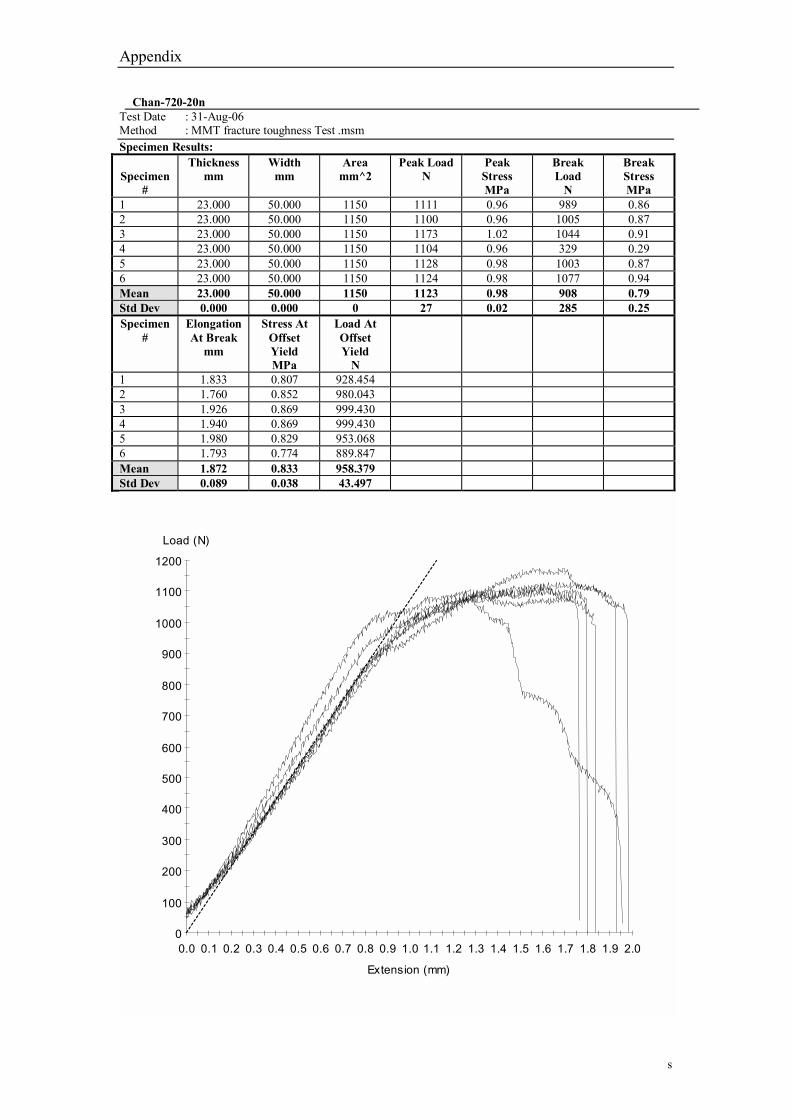
Appendix
s
Chan-720-20n Test Date : 31-Aug-06 Method : MMT fracture toughness Test .msm Specimen Results:
Specimen
#
Thickness mm
Width mm
Area mm^2
Peak Load N
Peak Stress MPa
Break Load
N
Break Stress MPa
1 23.000 50.000 1150 1111 0.96 989 0.86 2 23.000 50.000 1150 1100 0.96 1005 0.87 3 23.000 50.000 1150 1173 1.02 1044 0.91 4 23.000 50.000 1150 1104 0.96 329 0.29 5 23.000 50.000 1150 1128 0.98 1003 0.87 6 23.000 50.000 1150 1124 0.98 1077 0.94 Mean 23.000 50.000 1150 1123 0.98 908 0.79 Std Dev 0.000 0.000 0 27 0.02 285 0.25 Specimen
# Elongation At Break
mm
Stress At Offset Yield MPa
Load At Offset Yield
N
1 1.833 0.807 928.454 2 1.760 0.852 980.043 3 1.926 0.869 999.430 4 1.940 0.869 999.430 5 1.980 0.829 953.068 6 1.793 0.774 889.847 Mean 1.872 0.833 958.379 Std Dev 0.089 0.038 43.497
0
100
200
300
400
500
600
700
800
900
1000
1100
1200
0.0 0.1 0.2 0.3 0.4 0.5 0.6 0.7 0.8 0.9 1.0 1.1 1.2 1.3 1.4 1.5 1.6 1.7 1.8 1.9 2.0
Load (N)
Extension (mm)
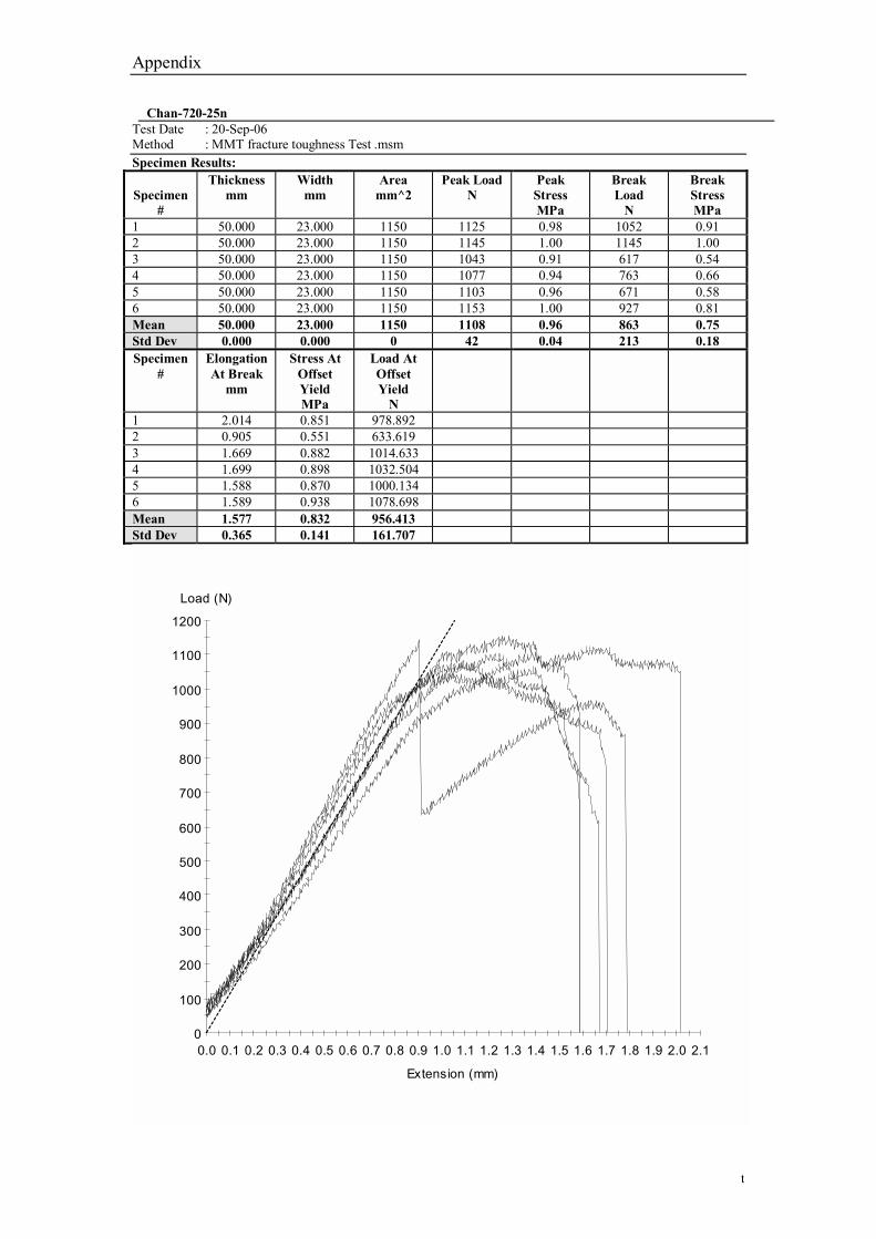
Appendix
t
Chan-720-25n Test Date : 20-Sep-06 Method : MMT fracture toughness Test .msm Specimen Results:
Specimen
#
Thickness mm
Width mm
Area mm^2
Peak Load N
Peak Stress MPa
Break Load
N
Break Stress MPa
1 50.000 23.000 1150 1125 0.98 1052 0.91 2 50.000 23.000 1150 1145 1.00 1145 1.00 3 50.000 23.000 1150 1043 0.91 617 0.54 4 50.000 23.000 1150 1077 0.94 763 0.66 5 50.000 23.000 1150 1103 0.96 671 0.58 6 50.000 23.000 1150 1153 1.00 927 0.81 Mean 50.000 23.000 1150 1108 0.96 863 0.75 Std Dev 0.000 0.000 0 42 0.04 213 0.18 Specimen
# Elongation At Break
mm
Stress At Offset Yield MPa
Load At Offset Yield
N
1 2.014 0.851 978.892 2 0.905 0.551 633.619 3 1.669 0.882 1014.633 4 1.699 0.898 1032.504 5 1.588 0.870 1000.134 6 1.589 0.938 1078.698 Mean 1.577 0.832 956.413 Std Dev 0.365 0.141 161.707
0
100
200
300
400
500
600
700
800
900
1000
1100
1200
0.0 0.1 0.2 0.3 0.4 0.5 0.6 0.7 0.8 0.9 1.0 1.1 1.2 1.3 1.4 1.5 1.6 1.7 1.8 1.9 2.0 2.1
Load (N)
Extension (mm)