Embed Size (px)
Citation preview

Fractional order statistic approximation fornonparametric conditional quantile inference
Matt Goldman∗ David M. Kaplan∗
September 28, 2015; first version December 15, 2011
Abstract
Using and extending fractional order statistic theory, we characterize the O(n−1)coverage probability error of the previously proposed confidence intervals for popula-tion quantiles using L-statistics as endpoints in Hutson (1999). We derive an analyticexpression for the n−1 term, which may be used to calibrate the nominal coveragelevel to get O(n−3/2 log(n)) coverage error. Asymptotic power is shown to be optimal.Using kernel smoothing, we propose a related method for nonparametric inference onconditional quantiles. This new method compares favorably with asymptotic normal-ity and bootstrap methods in theory and in simulations. Code is provided for bothunconditional and conditional inference.
JEL classification: C21Keywords: fractional order statistics, high-order accuracy, inference-optimal band-
width, kernel smoothing.
1 Introduction
Quantiles contain information about a distribution’s shape. Complementing the mean, they
capture heterogeneity, inequality, and other measures of economic interest. Nonparametric
conditional quantile models further allow arbitrary heterogeneity across regressor values.
This paper concerns nonparametric inference on quantiles and conditional quantiles. In
∗Goldman: Microsoft, [email protected]. Kaplan (corresponding author): Department of Eco-nomics, University of Missouri, [email protected]. We thank the co-editor (Oliver Linton), associateeditor, referees, and Yixiao Sun for helpful comments and references, and Patrik Guggenberger and AndresSantos for feedback improving the clarity of presentation. Thanks also to Brendan Beare, Karen Messer, andactive audience members at seminars and conferences. Thanks to Ruixuan Liu for providing and discussingcode from Fan and Liu (2015). This paper was previously circulated as parts of “IDEAL quantile inferencevia interpolated duals of exact analytic L-statistics” and “IDEAL inference on conditional quantiles.”
1

particular, we characterize the high-order accuracy of both Hutson’s (1999) L-statistic-based
confidence intervals (CIs) and our new conditional quantile CIs based thereon.
Conditional quantiles appear across diverse topics because they are fundamental statis-
tical objects. Studies of wages have looked at experience (Hogg, 1975), union membership
(Chamberlain, 1994), and inequality (Buchinsky, 1994). Other examples include models of
infant birthweight (Abrevaya, 2001), demand for alcohol (Manning et al., 1995), school qual-
ity and student outcomes (Eide and Showalter, 1998), and Engel curves (Alan et al., 2005;
Deaton, 1997, pp. 81–82), which we examine in our empirical application.
Previously, Hutson (1999) proposed CIs for quantiles based on fractional order statistics,
using L-statistics (linearly interpolating two order statistics) as endpoints. Although they
worked well and were used in practice, the CIs lacked formal proofs of accuracy and precision.
We provide these by deriving coverage probability error (CPE) and asymptotic power against
local alternatives, which is shown to be optimal.
The theoretical results we develop en route contribute to the fractional order statistic lit-
erature and provide the basis for inference on other objects of interest explored in Goldman
and Kaplan (2014) and Kaplan (2014). In particular, Theorem 2 tightly links the distri-
butions of L-statistics from the observed and ‘ideal’ (unobserved) fractional order statistic
processes, also showing a connection with the Brownian bridge process. Additionally, Lemma
7 provides precise PDF and PDF derivative approximations of the Dirichlet distribution (that
governs ideal fractional order statistics) in terms of the multivariate normal.
We derive an analytic leading n−1 term in the CPE for Hutson (1999) and provide a new
calibration to achieve O(n−3/2 log(n)) CPE. This is analogous to the Ho and Lee (2005a)
analytic calibration of the L-statistic CIs in Beran and Hall (1993), which similarly improves
CPE from O(n−1) to O(n−3/2).
High-order accuracy is most valuable in small samples. These may occur in experiments or
when the population itself is small (e.g., the 50 states in the U.S.). Perhaps most importantly,
even with moderate or large samples, nonparametric analysis can entail small local sample
2

sizes. For example, if n = 1024 and there are five binary regressors, then the smallest local
sample size cannot exceed 1024/25 = 32.
Our quantile CIs are closer to equal-tailed in finite samples than most. Symmetric and
equal-tailed CIs are first-order equivalent due to sample quantiles’ asymptotic normality,
but the higher-order differences can be important in finite samples, especially away from the
median. Viewing the CI as an interval estimator, this equal-tailed property is equivalent to
median unbiasedness, the virtues of which are discussed more in Section 3. Our theoretical
framework is not specific to equal-tailed CIs; modifications to achieve alternative optimal
properties are left to future work.
For nonparametric conditional quantile inference, we introduce an L-statistic-based ker-
nel method that smooths over continuous conditioning variables and also allows discrete
conditioning variables. Achieving CPE-optimal inference balances the aforementioned ana-
lytic CPE of our unconditional method and CPE from bias due to smoothing over continuous
regressors. We derive the optimal CPE and bandwidth rates, as well as a plug-in bandwidth
when the conditioning vector contains a single continuous component.
Our L-statistic method has theoretical and computational advantages over methods based
on normality or an unsmoothed bootstrap. The theoretical bottleneck for our approach is
the need to use a uniform kernel to apply our exact unconditional results. Nonetheless,
when the conditioning vector has one or two continuous components, our CPE is of smaller
order than that of normality or bootstrap methods, even if they assume infinite smoothness
of the conditional quantile function while we only assume two derivatives; see Section 4.3
for details. Our method also computes more quickly than existing methods (of reasonable
accuracy), handling even more challenging tasks in 10–15 seconds instead of minutes; see
Table 8.
Recent complementary work of Fan and Liu (2015) also concerns a “direct method” of
nonparametric inference on conditional quantiles. They use a limiting Gaussian process to
derive first-order accuracy in a general setting, whereas we use the finite-sample Dirichlet
3

process to achieve high-order accuracy in an iid setting. Fan and Liu (2015) also provide
uniform (over X) confidence bands. We suggest a confidence band from interpolating a
growing number of joint CIs, although it will take additional work to rigorously justify.
A different, more ad hoc confidence band described in Section 6 seems to perform well in
practice.
If applied to a local constant estimator with a uniform kernel and the same bandwidth,
the Fan and Liu (2015) approach is less accurate than ours due to the normal (instead of
beta) reference distribution and integer (instead of interpolated) order statistics in equation
(6). However, with other estimators like local polynomials, the Fan and Liu (2015) method
is not necessarily less accurate. We compare further in our simulations. One open question
is whether using our beta reference and interpolation can improve accuracy for the general
Fan and Liu (2015) method beyond the local constant estimator with a uniform kernel; our
Lemma 3 shows this will at least retain first-order accuracy.
The order statistic approach to quantile inference uses the idea of the probability integral
transform, which dates back to R. A. Fisher (1932), Karl Pearson (1933), and Neyman (1937).
For continuous Xiiid∼ F (·), F (Xi)
iid∼ Unif(0, 1). Each order statistic from such an iid uniform
sample has a known beta distribution for any sample size n. Order statistics may be regarded
as sample u-quantiles with index u ∈ (0, 1) such that (n+ 1)u is an integer. However, for a
given n, (n+ 1)u is fractional for almost all u ∈ (0, 1).
Though unobserved for non-integer indices, ‘ideal’ fractional order statistics1 for an iid
uniform sample jointly follow a particular Dirichlet process (Stigler, 1977), the marginal of
which is a beta distribution. We show that the L-statistic linearly interpolating consecutive
order statistics is well approximated by this beta distribution, with onlyO(n−1) error in CDF.
For example, the sampling distribution of the average of the 4th and 5th order statistics is
well approximated by the beta distribution of the 4.5th ideal fractional order statistic. This
O(n−1) bound on interpolation error is the key to formally justifying the L-statistic methods
1Technically, these are not statistics since they are not functions of the observed sample, but rathertheoretical constructs. Nonetheless, we follow the literature’s naming convention.
4

examined here and in other papers. AlthoughO(n−1) is an asymptotic claim, the interpolated
fractional order statistic cannot lie far from its unobserved counterpart even in small samples,
which is an advantage over methods more sensitive to asymptotic approximation error.
Many other approaches to one-sample quantile inference have been explored. With Edge-
worth expansions, Hall and Sheather (1988) and Kaplan (2015) obtain two-sided O(n−2/3)
CPE. With bootstrap, smoothing is necessary for high-order accuracy. This increases the
computational burden and requires good bandwidth selection in practice.2 See Ho and Lee
(2005b, §1) for a review of bootstrap methods. Bartlett-corrected smoothed empirical like-
lihood (Chen and Hall, 1993) also achieves nice theoretical properties, but with the same
caveats.
Other order statistic-based CIs dating back to Thompson (1936) are surveyed in David
and Nagaraja (2003, §7.1). Most closely related to Hutson (1999) is Beran and Hall (1993).
Like Hutson (1999), Beran and Hall (1993) linearly interpolate order statistics for CI end-
points, but with an interpolation weight based on the binomial distribution. Although their
proofs use expansions of the Rényi (1953) representation instead of fractional order statistic
theory, their n−1 CPE term (d1 in their appendix, or d2 for two-sided CIs) is identical to
that for Hutson (1999) other than the different weight value. Prior work (e.g., Bickel, 1967;
Shorack, 1972) has established asymptotic normality of L-statistics and convergence of the
sample quantile process to a Gaussian limit process, but the methods of Beran and Hall
(1993) and Hutson (1999) achieve higher-order accuracy.
The most apparent difference between the two-sided CIs of Beran and Hall (1993) and
Hutson (1999) is that the former are “symmetric” in terms of order statistic index (but not
length), whereas the latter are equal-tailed. This also allows Hutson (1999) to be computed
further into the tails; e.g., when n = 99, Hutson (1999) can compute a two-sided 95% CI
for quantiles in the range [0.036, 0.05], whereas Beran and Hall (1993) cannot. Additionally,
2For example, while achieving the impressive two-sided CPE of O(n−3/2), Polansky and Schucany (1997,p. 833) admit, “If this method is to be of any practical value, a better bandwidth estimation technique willcertainly be required.”
5

Goldman and Kaplan (2014) extend our fractional order statistic framework to justify high-
order accurate confidence intervals for two-sample quantile differences, interquantile ranges,
and other objects. Such extensions may be possible through the Rényi representation frame-
work, but we are unaware of such results, and the resulting methods would not have the
simple interpretation of using a Dirichlet reference distribution for the linearly interpolated
order statistics.
For nonparametric conditional quantile inference, in addition to the aforementioned Fan
and Liu (2015) approach, Chaudhuri (1991) derives the pointwise asymptotic normal distri-
bution of a local polynomial estimator. Qu and Yoon (2015) propose modified local linear
estimators of the conditional quantile process that converge weakly to a Gaussian process,
and they suggest using a conservative type of bias correction (that only enlarges a CI) to
deal with the asymptotic bias present when using a bandwidth of the MSE-optimal rate.
Alternatively, Fan and Liu (2015) may be applied to the Qu and Yoon (2015) estimator, ad-
dressing bias either through undersmoothing (as in the former paper’s simulations) or direct
bias correction (as in the latter). For comparison with the uniform (over quantiles) results in
Qu and Yoon (2015), the extension of our probability integral transform approach to uniform
confidence bands for the (unconditional) quantile process is in Goldman and Kaplan (2015).
Section 2 contains our theoretical results on fractional order statistic approximation,
which are applied to unconditional quantile inference in Section 3. Section 4 concerns our
new conditional quantile inference method. An empirical application and simulation results
are in Sections 5 and 6, respectively. Proofs absent from the text are collected in Appendix A,
and implementation notes are in Appendix B; further details of both are in the supplemental
appendix, along with additional simulations.
Notationally, φ(·) is the standard normal PDF, Φ(·) is the standard normal CDF, .=
should be read as “is equal to, up to smaller-order terms”; � as “has exact (asymptotic)
rate/order of” (same as “big theta” Bachmann–Landau notation, Θ(·)); and An = O(Bn)
as usual, ∃k < ∞ s.t. |An| ≤ Bnk for sufficiently large n. Acronyms used are those for
6

cumulative distribution function (CDF), confidence interval (CI), coverage probability (CP),
coverage probability error (CPE), and probability density function (PDF).
2 Fractional order statistic theory
In this section, we introduce notation and present our core theoretical results linking unob-
served ‘ideal’ fractional L-statistics with their observed counterparts.
Given an iid sample {Xi}ni=1 of draws from a continuous CDF denoted3 F (·), interest is
in Q(p) ≡ F−1(p) for some p ∈ (0, 1), where Q(·) is the quantile function. Let u ∈ (0, 1),
k ≡ bu(n+ 1)c, ε ≡ u(n+ 1)− k,
where b·c is the floor function and ε is the interpolation weight. The sample L-statistic
commonly associated with Q(u) is
QLX(u) ≡ (1− ε)Xn:k + εXn:k+1, (1)
where Xn:k denotes the kth order statistic (i.e., kth smallest sample value). While Q(u) is
latent and nonrandom, QLX(u) is a random variable, and QL
X(·) is a stochastic process, both
of which are observed for arguments varying over [1/(n+ 1), n/(n+ 1)].
Let Ξn ≡ {k/(n+ 1)}nk=1 denote the set of quantiles corresponding to the observed order
statistics. If u ∈ Ξn, then no interpolation is necessary and QLX(u) = Xn:k. As detailed in
Section 3, application of the probability integral transform yields exact coverage probability
of a CI endpoint Xn:k for Q(p): P (Xn:k < F−1(p)) = P (Un:k < p), where Un:k ≡ F (Xn:k) ∼
β(k, n + 1 − k) is equal in distribution to the kth order statistic from Uiiid∼ Unif(0, 1),
i = 1, . . . , n (Wilks, 1962, 8.7.4). However, we also care about u /∈ Ξn, in which case k
is fractional. To better handle such fractional order statistics, we will present a tight link
between the marginal distributions of the stochastic process QLX(·) and those of the analogous
3F will often be used with a random variable subscript to denote the CDF of that particular randomvariable. If no subscript is present, then F (·) refers to the CDF of X. Similarly for the PDF f(·).
7

‘ideal’ (I) process
QIX(·) ≡ F−1
(QIU(·)
), (2)
where QIU(·) is the ideal (I) uniform (U) fractional order statistic process. We use a tilde in
QIX(·) and QI
U(·) instead of the hat like in QLX(·) to emphasize that the former are unobserved,
whereas the latter is computable from the sample data.
This QIU(·) in (2) is a Dirichlet process (Ferguson, 1973; Stigler, 1977) on the unit interval
with index measure ν([0, t]) = (n+ 1)t. Its univariate marginals are
QIU(u) = Un:(n+1)u ∼ β
((n+ 1)u, (n+ 1)(1− u)
). (3)
The marginal distribution of(QIU(u1), QI
U(u2)− QIU(u1), . . . , QI
U(uk)− QIU(uk−1)
)for u1 <
· · · < uk is Dirichlet with parameters (u1(n+ 1), (u2 − u1)(n+ 1), . . . , (uk − uk−1)(n+ 1)).
Note that QIX(u) coincides with QL
X(u) for all u ∈ Ξn, differing only in its interpolation
between these points. Theorem 1 shows QIX(·) and QL
X(·) to be closely linked in probability.
Theorem 1. For any fixed δ > 0 and m > 0, define U δ ≡ {u ∈ (0, 1) | ∀ t ∈ (u −m,u +
m), f(F−1(t)) ≥ δ} and U δn ≡ U δ ∩ [ 1n+1
, nn+1
]; then, supu∈Uδn
∣∣∣QIX(u)− QL
X(u)∣∣∣ = Op(n
−1[log n]).
Although Theorem 1 motivates approximating the distribution of QLX(u) by that of
QIX(u), it is not relevant to high-order accuracy. In fact, its result is achieved by any
interpolation between Xn:k and Xn:k+1, not just QLX(u); in contrast, the high-order accuracy
we establish in Theorem 4 is only possible with precise interpolations like QLX(u).
Next, we consider the multivariate distribution of a vector of quantiles with fixed dimen-
sion J < ∞, where uj denotes an element in column vector u ∈ (0, 1)J . The joint PDF of
{QIU(uj)}Jj=1 evaluated at {xj}Jj=1 is Dirichlet with parameters (n+ 1)(uj − uj−1):
Γ(n+ 1)∏J+1j=1 Γ((n+ 1)(uj − uj−1))
(J+1∏j=1
(xj − xj−1)(n+1)(uj−uj−1)−1
),
where u0 ≡ 0, x0 ≡ 0, uJ+1 ≡ 1, and xJ+1 ≡ 1. Note that the Dirichlet more directly
8

describes the distribution of spacings QIU(uj)− QI
U(uj−1), rather than values QIU(uj).
We also consider the Gaussian approximation to the sampling distribution of order statis-
tics. It is well known that the centered and scaled empirical process for standard uniform
random variables converges to a Brownian bridge. For a Brownian bridge process B(·), we
define on u ∈ (0, 1) the additional stochastic processes
QBU (u) ≡ u+ n−1/2B(u) and QB
X(u) ≡ F−1(QBU (u)
).
Like the realizations of QIX(·) and QI
U(·), the realizations of these processes do not correspond
to observed data, but the distribution of QBX(u) provides a convenient approximation to the
distributions from the other processes. The vector QIU(u) has an ordered Dirichlet distri-
bution (i.e., the spacings between consecutive QIU(uj) follow a joint Dirichlet distribution),
while QBU (u) is multivariate Gaussian.
Lemma 7 in the appendix proves the close relationship between multivariate Dirichlet and
Gaussian PDFs and PDF derivatives for all values outside the tails (parts i and ii), which
are shown to have rapidly diminishing probability (parts iii and iv). To the best of our
knowledge, these are new results, and they facilitate the primary theoretical contributions
of our paper.
We use Lemma 7 to prove the close distributional link among linear combinations of
ideal, interpolated, and Gaussian-approximated fractional order statistics in Theorem 2.
Specifically, for arbitrary weight vector ψ ∈ RJ with non-zero elements ψj, we seek to
(distributionally) approximate
LL ≡J∑j=1
ψjQLX(uj) by LI ≡
J∑j=1
ψjQIX(uj), (4)
or alternatively by LB ≡J∑j=1
ψjQBX(uj).
For convenience and without loss of generality, we normalize ψ1 = 1.
Our assumptions for this section are now presented, followed by the main theoretical
9

result. Assumption A2 ensures that the first three derivatives of the quantile function are
uniformly bounded in neighborhoods of the quantiles, uj, which helps bound remainder terms
in the proofs. We use bold for vectors, underline for matrices, and φΣ(·) for the multivariate
normal PDF with mean 0 and covariance matrix Σ.
Assumption A1. Sampling is iid: Xiiid∼ F , i = 1, . . . , n.
Assumption A2. For each quantile uj, the PDF f(·) (corresponding to CDF F (·) in A1)
satisfies (i) f(F−1(uj)) > 0; (ii) f ′′(·) is continuous in some neighborhood of F−1(uj), i.e.,
f ∈ C2(Uδ(F−1(uj))) with Uδ(x) denoting some δ-neighborhood of point x ∈ R.
Theorem 2. Define V as the J × J matrix such that V i,j = min{ui, uj}(1 −max{ui, uj}),
and let
A ≡ diag{f(F−1(u))}, Vψ ≡ ψ′(A−1V A−1
)ψ, X0 ≡
J∑j=1
ψjF−1(uj).
As in (1), the εj ≡ (n + 1)uj − b(n + 1)ujc are interpolation weights. Let Assumption A1
hold, and let A2 hold at u. Given the definitions in (1), (2), and (4), the following results
hold uniformly over u = u + o(1).
(i) For a given constant K,
P
(LL < X0 + n−1/2K
)− P
(LI < X0 + n−1/2K
)=K exp{−K2/(2Vψ)}√
2πV3ψ
[J∑j=1
(ψ2j εj(1− εj)f [F−1(uj)]
2
)]n−1 +O(n−3/2 log(n)),
where the remainder is uniformly O(n−3/2 log(n)) over all K.
(ii) Uniformly over K,
supK∈R
[P
(LL < X0 + n−1/2K
)− P
(LI < X0 + n−1/2K
)]=
e−1/2√2πV2
ψ
[J∑j=1
(ψ2j εj(1− εj)f [F−1(uj)]
2
)]n−1 +O(n−3/2 log(n)),
10

and
supK∈R
∣∣∣∣P(LB < X0 + n−1/2K
)− P
(LI < X0 + n−1/2K
)∣∣∣∣ = O(n−1/2 log(n)).
The additional result for LB in part (ii) follows directly from the Dirichlet PDF approx-
imation in Lemma 8(ii), where the cubic term in the Taylor expansion around the mode is
O(n−1/2 log(n)).4
By the Cramér–Wold device, the vector QLX(u) converges in distribution to QI
X(u) up
to an O(n−1) term and to QBX(u) up to an O(n−1/2 log(n)) term. This could allow reliable
inference on more general finite-dimensional functionals of the quantile process. In the
remainder of this paper, attention is restricted to the class of linear combinations as in (4).
As shown in the proof, the CDF error in Theorem 2(ii) is proportional to
max
{[minj{uj}]−1, [min
j{1− uj}]−1
}.
This is consistent with the well-known additional difficulties of constructing confidences
intervals for “extreme quantiles” instead of “central quantiles.” We may remove this specific
term via analytic calibration, though a similar term likely remains.
3 Quantile inference: unconditional
For any quantile of interest p and confidence level 1 − α, we define uh(α) and ul(α) as
solutions to
α = P(QIU
(uh(α)
)< p), α = P
(QIU
(ul(α)
)> p), (5)
with QIU(u) ∼ β
((n + 1)u, (n + 1)(1 − u)
)from (3). These parallel (7) and (8) in Hutson
(1999).
One-sided CI endpoints are QLX(uh) or QL
X(ul), i.e., linearly interpolated fractional order
4A similar approximation error may follow from using the Bahadur remainder in Portnoy (2012).
11

statistics with index (n + 1)uh or (n + 1)ul. Two-sided CIs replace α with α/2 in (5)
and use both endpoints. This use of α/2 yields the equal-tailed property; more generally, for
t ∈ (0, 1), tα and (1−t)α can be used. Figure 1 visualizes an example. The beta distribution’s
mean is uh (or ul). Decreasing uh increases the probability mass in the shaded region below
u, while increasing uh decreases the shaded region, and vice-versa for ul. Consequently,
solving (5) is a simple numerical search problem.
0.0 0.2 0.4 0.6 0.8 1.0
01
23
45
u
Density
Determination of Lower Endpointn=11, u=0.65, α=0.1
α = 10%
ul = 0.42
0.0 0.2 0.4 0.6 0.8 1.0
01
23
45
u
Density
Determination of Upper Endpointn=11, u=0.65, α=0.1
α = 10%
uh = 0.84
Figure 1: Example of one-sided CI endpoint determination, n = 11, p = 0.65, α = 0.1. Left:the lower one-sided endpoint ul is such that the shaded region’s area is P
(QIU(ul) > p
)= α.
Right: similarly, uh solves P(QIU(uh) < p
)= α.
The CI endpoints converge to p at a root-n rate and may be approximated by quantiles
of a normal distribution, as in Lemma 3.
Lemma 3. Let z1−α denote the (1 − α)-quantile of a standard normal distribution, z1−α ≡
Φ−1(1− α). From the definitions in (5), the values ul(α) and uh(α) can be approximated as
ul(α) = p− n−1/2z1−α√p(1− p)− 2p− 1
6n(z2
1−α + 2) +O(n−3/2),
uh(α) = p+ n−1/2z1−α√p(1− p)− 2p− 1
6n(z2
1−α + 2) +O(n−3/2).
We first consider a lower one-sided CI for Q(p) based on the iid sample {Xi}ni=1. Using
12

(5), the 1− α CI from Hutson (1999) is
(−∞, QL
X
(uh(α)
)). (6)
Coverage probability is
P{Q(p) ∈
(−∞, QL
X(uh(α)))}
= P(QLX(uh(α)) > Q(p)
)Thm 2
= P(QIX(uh(α)) > Q(p)
)+εh(1− εh)z1−α exp{−z2
1−α/2}√2πuh(α)(1− uh(α))
n−1 +O(n−3/2 log(n))
= 1− α +εh(1− εh)z1−αφ(z1−α)
p(1− p)n−1 +O(n−3/2 log(n)),
where φ(·) is the standard normal PDF and the n−1 term is non-negative. Similar to the Ho
and Lee (2005a) calibration, we can remove the analytic n−1 term with the calibrated CI(−∞, QL
X
[uh(α +
εh(1− εh)z1−αφ(z1−α)
p(1− p)n−1
)]), (7)
which has CPE of O(n−3/2 log(n)). We follow convention and define CPE ≡ CP − (1 − α),
where CP is the actual coverage probability and 1− α the desired confidence level.
By parallel argument, Hutson’s (1999) uncalibrated upper one-sided and two-sided CIs
also have O(n−1) CPE, or O(n−3/2 log(n)) with calibration. For the upper one-sided case,
again using (5), the 1− α Hutson CI and our calibrated CI are respectively given by
(QLX [ul(α)],∞
), (8)(
QLX
[ul(α +
ε`(1− ε`)z1−αφ(z1−α)
p(1− p)n−1
)],∞), (9)
and for equal-tailed two-sided CIs,
(QLX
[ul(α/2)
], QL
X
[uh(α/2)
])and (10)(
QLX
[ul(α
2+ε`(1− ε`)z1−α/2φ(z1−α)
p(1− p)n−1
)], (11)
QLX
[uh(α
2+εh(1− εh)z1−α/2φ(z1−α)
p(1− p)n−1
)] ).
13

In all cases, the order n−1 CPE term is non-negative (indicating over-coverage).
For relatively extreme quantiles p (given n), the L-statistic method cannot be computed
because the (n+ 1)th (or zeroth) order statistic is needed. In such cases, our code uses the
Edgeworth expansion-based CI in Kaplan (2015). Alternatively, if bounds on X are known a
priori, they may be used in place of these “missing” order statistics to generate conservative
CIs. As n→∞, the range of computable quantiles approaches (0, 1).
To summarize CI construction, as in Hutson (1999) and implemented in our code:
1. Parameters: determine the sample size n, quantile of interest p ∈ (0, 1), and coverage
level 1− α. Optionally, use the calibrated α in (7), (8), or (11).
2. Endpoint index computation: solve for uh (for two-sided or lower one-sided CIs) and/or
ul (for two-sided or upper one-sided CIs) from (5), using (3). For a two-sided CI, replace
α in (5) with α/2.
3. CI construction: compute the lower and/or upper endpoints, respectively QLX(ul) and
QLX(uh), using (1).
The hypothesis tests corresponding to all the foregoing CIs achieve optimal asymptotic
power against local alternatives. The sample quantile is a semiparametric efficient estimator,
so it suffices to show that power is asymptotically first-order equivalent to that of the test
based on asymptotic normality. This is suggested by Lemma 3 and shown formally in the
appendix. Theorem 4 collects all of our results on coverage and power.
Theorem 4. Let zα denote the α-quantile of the standard normal distribution, and let εh =
(n + 1)uh(α)− b(n + 1)uh(α)c and ε` = (n + 1)ul(α)− b(n + 1)ul(α)c. Let Assumption A1
hold, and let A2 hold at quantile of interest p. Then, we have the following.
(i) The one-sided lower and upper CIs in (6) and (8) have coverage probability
1− α +ε(1− ε)z1−αφ(z1−α)
p(1− p)n−1 +O(n−3/2 log(n)),
with ε = εh for the former and ε = ε` for the latter.
14

(ii) The equal-tailed, two-sided CI in (10) has coverage probability
1− α +[εh(1− εh) + ε`(1− ε`)]z1−α/2φ(z1−α)
u(1− u)n−1 +O(n−3/2 log(n)).
(iii) The calibrated one-sided lower, one-sided upper, and two-sided equal-tailed CIs given
in (7), (8), and (11), respectively, have O(n−3/2 log(n)) CPE.
(iv) Against local sequence Dn = Q(p) + κn−1/2, asymptotic power of lower one-sided (l),
upper one-sided (u), and equal-tailed two-sided (t) CIs is
P ln(Dn)→ Φ(zα + S), Pun(Dn)→ Φ(zα − S), P tn(Dn)→ Φ(zα/2 + S
)+ Φ
(zα/2 − S
),
where S ≡ κf(F−1(p))/√p(1− p).
The equal-tailed property of our two-sided CIs is a type of median unbiasedness. If a
CI for scalar parameter θ has lower endpoint L and upper endpoint H, then an equal-tailed
CI is unbiased under the loss function L(θ, L, H) = max{0, θ − H, L − θ}, following the
definition in equation (5) of Lehmann (1951). Intuitively and mathematically, this is similar
to a median unbiased point estimator being above or below θ with equal probability. This
median unbiased property may be desirable (e.g., Andrews and Guggenberger, 2014, footnote
11), although it is different than the usual “unbiasedness” where a CI is the inversion of an
unbiased test.
More generally, in (10), we could replace ul(α/2) and uh(α/2) by ul(tα) and uh((1− t)α)
for t ∈ [0, 1], where t = 1/2 is currently used. Different values of t may achieve different
optimal properties, which we leave to future work.
15

4 Quantile inference: conditional
4.1 Setup and bias
Let QY |X(u;x) be the conditional u-quantile function of scalar outcome Y given conditioning
vector X ∈ X ⊂ Rd, evaluated at X = x. The sample {Yi, Xi}ni=1 is drawn iid. If the condi-
tional CDF FY |X(·) is strictly increasing and continuous at u, then FY |X(QY |X(u;x);x) = u.
For interior point x0 and quantile p ∈ (0, 1), interest is in QY |X(p;x0). Without loss of
generality, let x0 = 0.
If X is discrete so that P (X = 0) > 0, we can take all the observations with Xi = 0
and compute a CI from the corresponding Yi values, using the method in Section 3. If there
are Nn observations with Xi = 0, then the CPE from Theorem 4 is O(N−1n ) (uncalibrated).
This O(N−1n ) is O(n−1) even with dependence like strong mixing among the Xi (so that
Nn is almost surely of order n) as long as we have independent draws of Yi from the same
QY |X(·; 0).
If X is continuous (or Nn too small), we must include observations with Xi 6= 0. If
X contains mixed continuous and discrete components, then we can apply our method for
continuous X to each subsample corresponding to each unique value of the discrete subvector
of X. The asymptotic rates are unaffected by the presence of discrete variables (although
the finite-sample consequences may deserve more attention), so we focus on the case where
all components of X are continuous. Before proceeding, we present our assumptions and
definitions for this section. We continue using the normalization x0 = 0.
Definition 1 (local smoothness). Following Chaudhuri (1991, pp. 762–3): if, in a neigh-
borhood of the origin, function g(·) is continuously differentiable through order k, and its
kth derivatives are uniformly Hölder continuous with exponent γ ∈ (0, 1], then g(·) has local
smoothness of degree s = k + γ.
Assumption A3. Sampling of (Yi, X′i)′ is iid, for continuous scalar Yi and continuous vector
Xi ∈ X ⊆ Rd. The point of interest X = 0 is in the interior of X , and the quantile of interest
16

is p ∈ (0, 1).
Assumption A4. The marginal density of X, denoted fX(·), satisfies fX(0) > 0 and has
local smoothness sX = kX + γX > 0.
Assumption A5. For all u in a neighborhood of p, QY |X(u; ·) (as a function of the second
argument) has local smoothness5 sQ = kQ + γQ > 0.
Assumption A6. As n→∞, the bandwidth satisfies (i) h→ 0, (ii) nhd/[log(n)]2 →∞.
Assumption A7. For all u in a neighborhood of p and all x in a neighborhood of the origin,
fY |X(QY |X(p; 0); 0
)is uniformly bounded away from zero.
Assumption A8. For all y in a neighborhood of QY |X(p; 0) and all x in a neighborhood
of the origin, fY |X(y;x) has a second derivative in its first argument (y) that is uniformly
bounded and continuous in y, having local smoothness sY = kY + γY > 2.
For continuous Xi, the “effective sample” includes observations with Xi ∈ Ch, where h
is the bandwidth and Ch = [−h, h] if d = 1. For d > 1, Ch is a hypersphere or hypercube,
similar to Chaudhuri (1991, pp. 762–3). Definition 2 refers to
Ch ≡ {x : x ∈ Rd, ‖x‖ ≤ h}, (12)
Nn ≡ #({Yi : Xi ∈ Ch, 1 ≤ i ≤ n}
). (13)
Definition 2 (effective sample). Let h denote the bandwidth and p ∈ (0, 1) the quantile
of interest. The “effective sample” consists of Yi values from observations with Xi inside
the window Ch ⊂ Rd defined in (12), wherein ‖ · ‖ denotes any norm on Rd (e.g., L2 norm
to get hypersphere Ch, L∞ norm for hypercube). The “effective sample size” is Nn as in
(13). Additionally, let QY |X(p;Ch) be the p-quantile of Y given X ∈ Ch, satisfying p =
P(Y < QY |X(p;Ch) | X ∈ Ch
).
5Our sQ corresponds to variable p in Chaudhuri (1991); Bhattacharya and Gangopadhyay (1990) usesQ = 2 and d = 1.
17

Given fixed values of n and h, Assumption A3 implies that the Yi in the effective sample
are independent and identically distributed, which is needed to apply Theorem 4. However,
they do not have the quantile function of interest, QY |X(·; 0), but rather the slightly biased
QY |X(·;Ch). This is like drawing a global (any Xi) iid sample of wages, Yi, and restricting
it to observations in Japan (X ∈ Ch) when our interest is only in Tokyo (X = 0): our
restricted Yi constitute an iid sample from Japan, but the p-quantile wage in Japan may
differ from that in Tokyo. Assumptions A4–A6(i) and A8 are necessary for the calculation
of this bias, QY |X(p;Ch) − QY |X(p; 0), in Lemma 5. Assumptions A6(ii) and A7 (and A3)
ensure Nna.s.→ ∞. Assumptions A7 and A8 are conditional versions of Assumptions A2(i) and
A2(ii), respectively. Their uniformity ensures uniformity of the remainder term in Theorem
4, accounting for the fact that the local sample’s distribution, FY |Ch , changes with n (through
h and Ch).
From A6(i), asymptotically Ch is entirely contained within the neighborhoods implicit
in A4, A5, and A8. This in turn allows us to examine only a local neighborhood around
quantile of interest p (e.g., as in A5) since the CI endpoints converge to the true value at a√Nn rate. Reassuringly, the optimal bandwidth rate derived in Section 4.2 turns out to be
inside the bounds in A6.
Definition 3 (steps for conditional L-statistic method). Given {Xi, Yi}ni=1 where vector Xi
contains only continuously distributed variables, bandwidth h > 0, quantile p ∈ (0, 1), and
desired coverage probability 1− α, first Ch and Nn are calculated as in Definition 2. Using
the Yi from observations with Xi ∈ Ch, a p-quantile CI is constructed as in Hutson (1999) if
computable or Kaplan (2015) otherwise. If additional discrete conditioning variables exist,
this method is repeated separately for each combination of discrete conditioning values (e.g.,
once for males and once for females). This procedure may be repeated for any number of
x0. For the bandwidth, we recommend the formulas in Section 4.4.
The Xi being iid helps guarantee that Nn is almost surely of order nhd. The hd comes
from the volume of Ch. Larger h lowers CPE via Nn but raises CPE via bias. This tradeoff
18

determines the optimal rate at which h → 0 as n → ∞. Using Theorem 4 and additional
results on CPE from bias below, we determine the optimal value of h.
Since our conditional quantile CI uses the subsample of Yi with Xi ∈ Ch rather than
Xi = 0, our CI is constructed for the biased conditional quantile QY |X(p;Ch) (from Definition
2) rather than for QY |X(p; 0). The bias characterized in Lemma 5 is the difference between
these two population conditional quantiles.
Lemma 5. Define b ≡ min{sQ, sX+1, 2} and Bh ≡ QY |X(p;Ch)−QY |X(p; 0). If Assumptions
A4, A5, A6(i), and A8 hold, then the bias is of order
|Bh| = O(hb). (14)
With A4 and A5 strengthened to kX ≥ 1 and kQ ≥ 2, the bias is O(h2) with remainder o(h2).
With further strengthening to kX ≥ 2 and kQ ≥ 3, the bias remains O(h2), but the remainder
sharpens to o(h3).
With d = 1, and defining
Q(0,1)Y |X (p; 0) ≡ ∂
∂xQY |X(p;x)
∣∣∣∣x=0
, Q(0,2)Y |X (p; 0) ≡ ∂2
∂x2QY |X(p;x)
∣∣∣∣x=0
, ξp ≡ QY |X(p; 0),
f(0,1)Y |X (y; 0) ≡ ∂
∂xfY |X(y;x)
∣∣∣∣x=0
, f(1,0)Y |X (ξp; 0) ≡ ∂
∂yfY |X(y; 0)
∣∣∣∣y=ξp
,
and similarly for F (0,1)Y |X (ξp; 0) and F (0,2)
Y |X (ξp; 0), the bias is
Bh =h2
6
{2Q
(0,1)Y |X (p; 0)f ′X(0)/fX(0) +Q
(0,2)Y |X (p; 0)
+ 2f(0,1)Y |X (ξp; 0)Q
(0,1)Y |X (p; 0)/fY |X(ξp; 0)
+ f(1,0)Y |X (ξp; 0)
[Q
(0,1)Y |X (p; 0)
]2
/fY |X(ξp; 0)
}+R
= −h2fX(0)F
(0,2)Y |X (ξp; 0) + 2f ′X(0)F
(0,1)Y |X (ξp; 0)
6fX(0)fY |X(ξp; 0)+R,
where R = o(h2) or R = o(h3) as discussed.
The dominant term in the bias when kX ≥ 1, kQ ≥ 2, and d = 1 is the same as the
19

bias in Bhattacharya and Gangopadhyay (1990), who derive it using different arguments.
The maximum value b = 2 (making the bias at least O(h2)) is due to our implicit use of a
uniform kernel, which is a second-order kernel. Consequently, there is no benefit to having
smoothness greater than (sQ, sX , sY ) = (2, 1, 1) + ε for arbitrarily small ε > 0.
4.2 Optimal CPE order
The CPE-optimal bandwidth minimizes the sum of the two dominant high-order CPE terms.
It must be small enough to control the O(hb +Nnh2b) (two-sided) CPE from bias, but large
enough to control the O(N−1n ) CPE from applying the unconditional L-statistic method. As
before, CPE ≡ CP − (1 − α), so CPE is positive when there is over-coverage and negative
when there is under-coverage. This means the equivalent hypothesis test is size distorted
when CPE is negative. The following theorem summarizes optimal bandwidth and CPE
results.
Theorem 6. Let Assumptions A3–A8 hold, and define b ≡ min{sQ, sX+1, 2}. The following
results are for the method in Definition 3 when Hutson (1999) is used.
For a one-sided CI, the bandwidth h∗ minimizing CPE has rate h∗ � n−3/(2b+3d). This
corresponds to overall CPE of O(n−2b/(2b+3d)).
For two-sided inference, the optimal bandwidth rate is h∗ � n−1/(b+d), and the optimal
CPE is O(n−b/(b+d)). If Kaplan (2015) is used instead of Hutson (1999), then h∗ � n−5/(5d+6b)
and CPE is O(n−4b/(5d+6b)).
Using the calibration in Section 3, the nearly (up to log(n)) CPE-optimal two-sided band-
width rate is h∗ � n−5/(4b+5d), yielding CPE of O(n−6b/(4b+5d) log(n)
). The nearly optimal
calibrated one-sided bandwidth rate is h∗ � n−2/(b+2d), yielding CPE of O(n−3b/(2b+4d) log(n)
).
If used in a semi-nonparametric (e.g., partially linear) model like in Fan and Liu (2015),
depending on d, the CPE-optimal bandwidth and CPE rates may differ from Theorem 6.
For example, with d = 1, b = 2, and a two-sided CI, the bias from Lemma 5 with h � n−1/3
20

is O(h2) = O(n−2/3). Since there is larger-order bias from plugging in a root-n normal
estimator of the parametric part of the model, the CPE-optimal h will be smaller, and
the overall CPE larger. Precise characterization of the optimal h and CPE rates in semi-
nonparametric models would require a statement about β such as P (|β − β| > nδ) = O(nη),
where the new bias order is nδ and the overall CPE is of order nη or larger. For now, we
note that our method is at least first-order accurate in such models, with Lemma 3 explicitly
connecting our method to results in Fan and Liu (2015).
4.3 CPE comparison with other methods
Theorem 6 suggests that for the most common values of dimension d and most plausible
values of smoothness sQ, our method is preferred to inference based on asymptotic normal-
ity (or, equivalently, unsmoothed bootstrap) with a local polynomial estimator. Only our
uncalibrated method is compared here.
The only chance for normality to yield smaller CPE is to greatly reduce bias by using a
very large local polynomial. However, our method has smaller CPE when d = 1 or d = 2
even if sQ =∞.
In finite samples, the normality approach may have additional error from estimation of
the asymptotic variance, which includes the probability density of the error term at zero as
discussed in Chaudhuri (1991, pp. 764–766). Additionally, large local polynomials cannot
perform well unless there is a large local sample size.
For the local polynomial approach, the CPE-optimal bandwidth and optimal CPE can
be derived from the results in Chaudhuri (1991). We balance the CPE from the bias with
additional CPE from the Bahadur remainder from his Theorem 3.3(ii). The CPE from bias
is of order N1/2n hsQ . Chaudhuri (1991, Thm. 3.3) gives a Bahadur-type expansion of the
local polynomial quantile regression estimator that has remainder Rn
√Nn = O(N
−1/4n ) (up
to log terms) as in Bahadur (1966), but recently Portnoy (2012) has shown that the CPE is
nearly O(N−1/2n ) in such cases. Solving N1/2
n hsQ � N−1/2n � (nhd)−1/2 yields h∗ � n−1/(sQ+d)
21

and optimal CPE (nearly) O(√NnBn) = O(N
−1/2n ) = O(n−sQ/(2sQ+2d)).
1 2 3 4 5
−1.
0−
0.8
−0.
6−
0.4
−0.
20.
0sQ = 2
d
CP
E e
xpon
ent
L−statL−stat (calib)C91
1 2 3 4 5 6 7
05
1015
sQ needed to match L−stat CPE
d
s Q
020
040
060
080
0
Num
ber
of p
olyn
omia
l ter
ms
L−statalwaysbetter
sQ
terms
Figure 2: Two-sided CPE comparison between new (“L-stat”) method and the local polyno-mial asymptotic normality method based on Chaudhuri (1991). Left: with sQ = 2, writingCPE as nκ, comparison of κ for different methods and different values of d. Right: requiredsmoothness sQ for the local polynomial normality-based CPE to match that of L-stat, aswell as the corresponding number of terms in the local polynomial, for different d.
As illustrated in the left panel of Figure 2, if sQ = 2 (one Lipschitz-continuous derivative),
then the optimal CPE from asymptotic normality is nearly O(n−2/(4+2d)), which is always
larger than our method’s CPE. With d = 1, this is n−1/3, significantly larger than our n−2/3
(one-sided: n−4/7). With d = 2, n−1/4 is larger than our n−1/2 (one-sided: n−2/5). It remains
larger for all d, even for one-sided inference, since the bias is the same for both methods and
the unconditional L-statistic inference is more accurate than normality.
From another perspective, as in the right panel of Figure 2: what amount of smoothness
(and local polynomial degree) is needed for asymptotic normality to match our method’s
CPE? For the most common cases of d ∈ {1, 2} (one-sided: d = 1), normality is worse even
with infinite smoothness. With d = 3 (one-sided: d = 2), normality needs sQ ≥ 12 to match
our CPE. If n is large, then maybe such a high degree (kQ ≥ 11) local polynomial will be
appropriate, but often it is not. Interaction terms are required, so an 11th-degree polynomial
has∑kQ+d−1
T=d−1
(Td−1
)= 364 terms. As d → ∞, the required smoothness approaches sQ = 4
22

(one-sided: 8/3) from above, though again the number of terms in the local polynomial
grows with d as well as kQ and may thus still be prohibitive in finite samples.
Basic bootstraps claim no refinement over asymptotic normality, so the foregoing dis-
cussion also applies to such methods. Without using smoothed or m-out-of-n bootstrap,
which require additional smoothing parameter choice and computation time, Studentization
offers no CPE improvement. Gangopadhyay and Sen (1990) examine the bootstrap per-
centile method for a uniform kernel (or nearest neighbor) estimator with d = 1 and sQ = 2,
but they only show first-order consistency. Based on their (2.14), the optimal error seems
to be O(n−1/3) when h � n−1/3 (matching our derivation from Chaudhuri (1991)) to bal-
ance the bias and remainder terms, improved by Portnoy (2012) from O(n−2/11) CPE when
h � n−3/11.
4.4 Plug-in bandwidth
Keeping track of terms more carefully, we can solve for not just the rate of the CPE-optimal
bandwidth, but its value. To avoid recursive dependence on ε (the interpolation weight), we
fix its value. This does not achieve the theoretical optimum, but it remains close even in small
samples and seems to work well in practice. The CPE-optimal bandwidth value derivation is
shown for d = 1 in Appendix B, a plug-in version of which is implemented in our code. For
reference, the plug-in bandwidth expressions are collected here. Standard normal quantiles
are denoted, for example, z1−α for the (1 − α)-quantile such that Φ(z1−α) = 1 − α. We let
Bh denote the estimator of bias term Bh; fX the estimator of fX(x0); f ′X the estimator of
f ′X(x0); F (0,1)Y |X the estimator of F (0,1)
Y |X (ξp;x0); and F (0,2)Y |X the estimator of F (0,2)
Y |X (ξp;x0), where
ξp ≡ QY |X(p;x0).
We recommend the following when d = 1.
23

• For one-sided inference, let
h+− = n−3/7
z1−α
3[p(1− p)fX
]1/2{fXF
(0,2)Y |X + 2f ′XF
(0,1)Y |X
}
2/7
, (15)
h++ = −0.770h+−. (16)
For lower one-sided inference, h+− should be used if Bh < 0, and h++ otherwise.
For upper one-sided inference, h++ should be used if Bh < 0, and h+− otherwise.
Alternatively, always using |h++| is simpler but will sometimes be conservative.
• For two-sided inference on the median,
h = n−1/3∣∣∣fXF (0,2)
Y |X + 2f ′XF(0,1)Y |X
∣∣∣−1/3
. (17)
• For two-sided inference with general p ∈ (0, 1), and equivalent to (17) with p = 1/2,
h = n−1/3
(Bh/|Bh|)(1− 2p) +√
(1− 2p)2 + 4
2∣∣∣fXF (0,2)
Y |X + 2f ′XF(0,1)Y |X
∣∣∣1/3
. (18)
We also suggest (and implement in our code) shifting toward a larger bandwidth as
n → ∞. Once the absolute differences in CPE are small, a larger bandwidth (that still
maintains o(1) CPE) is preferable since it yields shorter CIs. However, the usual question
of how big n needs to be remains to be formalized. Currently, we use a coefficient of
max{1, n/1000}5/60 that keeps the CPE-optimal bandwidth for n ≤ 1000 and then moves
toward a n−1/20 undersmoothing of the MSE-optimal bandwidth rate, as in Fan and Liu
(2015).
4.5 Joint confidence intervals and a possible uniform band
Beyond the pointwise CIs in Definition 3, the usual Bonferroni adjustment α/m gives joint
CIs over m different values of x0. If the Ch are mutually exclusive, then the local samples
are independent due to Assumption A3, and the adjustment can be refined to 1− (1−α)1/m,
24

which maintains exact joint coverage (not conservative like Bonferroni).
The number of such mutually exclusive windows grows as n→∞, which may be helpful
for constructing a uniform confidence band. If Assumption A5 is strengthened to a uniform
bound on the second derivative (wrt X) of the conditional quantile function, then the lo-
cal bandwidths have a common asymptotic rate, h, and there can be order 1/h mutually
exclusive local samples. The error from a linear approximation of the conditional quantile
function over a span of h is O(h2). This is smaller than the length of the CIs, which is order
1/√nhd = h when using the CPE-optimal bandwidth rate h � n−1/(2+d) for two-sided CIs
from Theorem 6 with b = 2.
The growing number of CIs is not problematic given independent sampling, but the fact
that α→ 0 (at rate h) has not been rigorously treated. We leave such proof to future work,
suggesting due caution in applying the uniform band until then. As discussed in Section
6, a Hotelling (1939) tube-based calibration of α also appears to yield reasonable uniform
confidence bands, but it has even less formal justification.
5 Empirical application
We present an application of our L-statistic inference to Engel (1857) curves. Code is
available from the latter author’s website, and the data are publicly available.
Banks et al. (1997) argue that a linear Engel curve is sufficient for certain categories of
expenditure, while adding a quadratic term suffices for others. Their Figure 1 shows non-
parametrically estimated mean Engel curves (budget share W against log total expenditure
ln(X)) with 95% pointwise CIs at the deciles of the total expenditure distribution, using a
subsample of 1980–1982 U.K. Family Expenditure Survey (FES) data.
We present a similar examination, but for quantile Engel curves in the 2001–2012 U.K.
Living Costs and Food Surveys (Office for National Statistics and Department for Environ-
ment, Food and Rural Affairs, 2012), which is a successor to the FES. We examine the same
25

four categories as in the original analysis: food; fuel, light, and power (“fuel”); clothing and
footwear (“clothing”); and alcohol. We use the subsample of households with one adult male
and one adult female (and possibly children) living in London or the South East, leaving
8,528 observations. Expenditure amounts are adjusted to 2012 nominal values using annual
CPI data.6
Table 1: L-statistic 99% CIs for various quantiles (p) of the budget share distribution, fordifferent categories of expenditure described in the text.
Category p = 0.5 p = 0.75 p = 0.9food (0.1532,0.1580) (0.2095,0.2170) (0.2724,0.2818)fuel (0.0275,0.0289) (0.0447,0.0470) (0.0692,0.0741)
clothing (0.0135,0.0152) (0.0362,0.0397) (0.0697,0.0761)alcohol (0.0194,0.0226) (0.0548,0.0603) (0.1012,0.1111)
Table 1 shows unconditional L-statistic CIs (Hutson, 1999) for various quantiles of the
budget share distributions for the four expenditure categories. (Due to the sample size,
calibrated CIs are identical at the precision shown.) These capture some population features,
but the conditional quantiles are of more interest.
Figure 3 is comparable to Figure 1 of Banks et al. (1997) but with 90% joint (over all nine
expenditure levels) CIs instead of 95% pointwise CIs, alongside quadratic quantile regression
estimates. Joint CIs are more intuitive for assessing the shape of a function since they jointly
cover all corresponding points on the true curve with 90% probability, rather than any given
single point. The CIs are interpolated only for visual convenience. Although some of the joint
CI shapes do not look quadratic, the only cases where the quadratic fit lies outside one of
the intervals are for alcohol at the conditional median and clothing at the conditional upper
quartile, and neither is a radical departure. With a 90% confidence level and 12 confidence
sets, we would not be surprised if one or two did not cover the true quantile Engel curve
completely. Importantly, the CIs are relatively precise, too; the linear fit is rejected in 8 of
12 cases. Altogether, this evidence suggests that the benefits of a quadratic (but not linear)
6http://www.ons.gov.uk/ons/datasets-and-tables/data-selector.html?cdid=D7BT&dataset=mm23&table-id=1.1
26

6.0 6.5 7.0
0.10
0.15
0.20
0.25
0.30
0.35
Joint: Food
log expenditure
budg
et s
hare
●
●
●
● ●
●●
●
●
●
●
●
● ●
●
●●
●
● 0.50−quantile0.75−quantile0.90−quantile
6.0 6.5 7.0
0.02
0.04
0.06
0.08
0.10
Joint: Fuel, light, and power
log expenditure
budg
et s
hare
●
●
●●
●
●● ●
●
●
●
●
●
●●
●●
●
● 0.50−quantile0.75−quantile0.90−quantile
6.0 6.5 7.0
0.00
0.02
0.04
0.06
0.08
0.10
0.12
Joint: Clothing/footwear
log expenditure
budg
et s
hare
●
●
● ●●
● ●●
●● ●●
●●
● ●●
●
● 0.50−quantile0.75−quantile0.90−quantile
6.0 6.5 7.0
0.00
0.05
0.10
0.15
0.20
Joint: Alcohol
log expenditure
budg
et s
hare
●●
●●
●●
● ●●
●●
● ●
●●
● ●●
● 0.50−quantile0.75−quantile0.90−quantile
Figure 3: Joint (over the nine expenditure levels) 90% confidence intervals for quantile Engelcurves: food (top left), fuel (top right), clothing (bottom left), and alcohol (bottom right).
27

approximation probably outweigh the cost of approximation error.
The L-statistic joint CIs (“L-stat”) in Figure 4 are the same as those for p = 0.5 and
p = 0.9 in Figure 3, but now a nonparametric (instead of quadratic) conditional quantile
estimate is shown, along with joint CIs from Fan and Liu (2015). The L-stat CIs are generally
shorter, but there can be exceptions, as seen especially in the bottom right graph. Of course,
shorter is not better if coverage probability is sacrificed; we explore both properties in the
simulations of Section 6.
6.0 6.5 7.0
0.10
0.15
0.20
0.25
0.30
0.35
Joint: Food (subsample of 8528)
log expenditure
budg
et s
hare
●
●●
●●
●●
●●
●
●●
● ●
●
●
●●
●
●
●
● ●
●
●
●●
●
●
●
●●
●
●
●
●
●
estimateFan−LiuL−stat
6.0 6.5 7.0
0.02
0.04
0.06
0.08
0.10
Joint: Fuel, light, and power (subsample of 8528)
log expenditure
budg
et s
hare
●
●●
●●
●● ●
●
●
●
●
●
●●
●●
●
●
●
●
●
● ●
● ●
●
●
●
●
●
●●
● ●
●
●
estimateFan−LiuL−stat
6.0 6.5 7.0
0.00
0.02
0.04
0.06
0.08
0.10
0.12
Joint: Clothing/footwear (subsample of 8528)
log expenditure
budg
et s
hare
●
●
● ● ● ● ● ● ●●●
● ● ● ●●
● ●
●
●
●●
●
● ●
●●
●●
●●
●
●●
● ●
●
estimateFan−LiuL−stat
6.0 6.5 7.0
0.00
0.05
0.10
0.15
0.20
Joint: Alcohol (subsample of 8528)
log expenditure
budg
et s
hare
●●
● ●
● ● ● ●●
●
●● ●
● ● ● ●●
● ● ●
●
●
● ●●
●● ●
●
●●
●●
●
●
●
estimateFan−LiuL−stat
Figure 4: Joint (over the nine expenditure levels) 90% confidence intervals for quantile Engelcurves, p = 0.5 and p = 0.9: food (top left), fuel (top right), clothing (bottom left), andalcohol (bottom right).
28

6 Simulation study
Code for our L-statistic methods in R is available on the latter author’s website,7 as is the
simulation code.
6.1 Unconditional simulations
We compare two-sided unconditional CIs from the following methods: “L-stat” from Section
3, originally in Hutson (1999); “BH” from Beran and Hall (1993); “Norm” using the sample
quantile’s asymptotic normality and kernel-estimated variance; “K15” from Kaplan (2015);
and “BStsym,” a symmetric Studentized bootstrap (99 draws) with bootstrapped variance
(100 draws). (Other bootstraps were consistently worse in terms of coverage: (asymmetric)
Studentized bootstrap, and percentile bootstrap with and without symmetry.)
Unless otherwise noted, α = 0.05 and 10,000 replications of each DGP were simulated.
Overall, L-stat and BH have the most accurate coverage probability (CP), avoiding under-
coverage while maintaining shorter length than other methods achieving at least 95% CP.
Near the median, L-stat and BH are nearly identical. In the tails, L-stat is shorter than BH
for some distributions and comes closer to being equal-tailed. Farther into the tails, BH is
not computable, but L-stat maintains a favorable combination of CP and length compared
with other methods.
Table 2 shows nearly exact CP for both L-stat and BH when n = 25 and p = 0.5. The
normal CI can be slightly shorter, but it under-covers. The bootstrap has only slight under-
coverage, and K15 none, but their CIs are longer than L-stat and BH. In the Supplemental
Appendix, results are shown for additional distributions and for n = 9, but the qualitative
points are the same.
Table 3 shows a case in the lower tail with n = 99 where BH cannot be computed (because
it needs the zeroth order statistic). Even then, L-stat’s CP remains almost exact, and it is7In the code, if Nn is not large enough to compute Hutson (1999) at quantile p, then the method in
Kaplan (2015) is used instead. If Nn is too small even for Kaplan (2015), then a method based on extremevalue theory is recommended instead.
29

Table 2: Coverage probability and median CI length, 1 − α = 0.95; various n, p, anddistributions of Xi (F ) shown in table. “Too high” is the proportion of simulations in whichthe lower endpoint was above the true value, F−1(p), and “too low” is the proportion whenthe upper endpoint was below F−1(p).
n p F Method CP Too low Too high Length25 0.5 Normal L-stat 0.953 0.022 0.025 0.9925 0.5 Normal BH 0.955 0.021 0.024 1.0025 0.5 Normal Norm 0.942 0.028 0.030 1.0225 0.5 Normal K15 0.971 0.014 0.015 1.1925 0.5 Normal BStsym 0.942 0.028 0.030 1.1325 0.5 Uniform L-stat 0.953 0.022 0.025 0.3725 0.5 Uniform BH 0.954 0.021 0.025 0.3725 0.5 Uniform Norm 0.908 0.046 0.046 0.3525 0.5 Uniform K15 0.963 0.018 0.020 0.4425 0.5 Uniform BStsym 0.937 0.031 0.032 0.4525 0.5 Exponential L-stat 0.953 0.024 0.023 0.7925 0.5 Exponential BH 0.954 0.024 0.022 0.8025 0.5 Exponential Norm 0.924 0.056 0.020 0.7525 0.5 Exponential K15 0.968 0.022 0.010 0.9625 0.5 Exponential BStsym 0.941 0.039 0.020 0.93
Table 3: Coverage probability and median CI length, as in Table 2.
n p F Method CP Too low Too high Length99 0.037 Normal L-stat 0.951 0.023 0.026 1.0299 0.037 Normal BH NA NA NA NA99 0.037 Normal Norm 0.925 0.016 0.059 0.8399 0.037 Normal K15 0.970 0.009 0.021 1.5599 0.037 Normal BStsym 0.950 0.020 0.030 1.2099 0.037 Cauchy L-stat 0.950 0.022 0.028 39.3799 0.037 Cauchy BH NA NA NA NA99 0.037 Cauchy Norm 0.784 0.082 0.134 18.9099 0.037 Cauchy K15 0.957 0.002 0.041 36.5599 0.037 Cauchy BStsym 0.961 0.002 0.037 48.7799 0.037 Uniform L-stat 0.951 0.024 0.026 0.0799 0.037 Uniform BH NA NA NA NA99 0.037 Uniform Norm 0.990 0.000 0.010 0.1299 0.037 Uniform K15 0.963 0.028 0.009 0.1199 0.037 Uniform BStsym 0.924 0.053 0.022 0.08
30

closest to being equal-tailed. The normal CI under-covers for the first two F and is almost
twice as long as the L-stat CI for the third F . BStsym has less under-coverage, and K15
none, but both are generally longer than L-stat. Again, results for additional F are in the
Supplemental Appendix, with similar patterns, as well as results for n = 99 and p = 0.05 or
p = 0.95, where again BH cannot be computed.
Table 4: Coverage probability and median CI length, as in Table 2.
n p F Method CP Too low Too high Length25 0.2 Normal L-stat 0.956 0.023 0.021 1.1825 0.2 Normal BH 0.967 0.028 0.006 1.3325 0.2 Normal Norm 0.944 0.011 0.045 1.1325 0.2 Normal K15 0.952 0.006 0.042 1.4225 0.2 Normal BStsym 0.944 0.022 0.034 1.3425 0.2 Cauchy L-stat 0.960 0.024 0.016 5.0525 0.2 Cauchy BH 0.965 0.028 0.006 7.8725 0.2 Cauchy Norm 0.909 0.014 0.077 2.4325 0.2 Cauchy K15 0.946 0.001 0.053 4.0025 0.2 Cauchy BStsym 0.959 0.005 0.036 5.1825 0.2 Uniform L-stat 0.952 0.022 0.026 0.2925 0.2 Uniform BH 0.963 0.026 0.010 0.3025 0.2 Uniform Norm 0.960 0.006 0.034 0.3325 0.2 Uniform K15 0.953 0.015 0.032 0.3925 0.2 Uniform BStsym 0.930 0.042 0.028 0.35
Table 4 shows a case with p = 0.2 (away from the median) where BH can be computed.
The patterns among the normal, K15, and BStsym CIs are similar to before. L-stat and BH
both attain 95% CP in each case, but L-stat is much closer to equal-tailed, and L-stat is
shorter or the same length. The Supplemental Appendix contains additional, similar results.
Table 5 compares the original two-sided CI in equation (10) with the calibrated (“Calib”)
version in (11). Even with small n, the true differences are small, so we use a larger number
of replications (105) to reduce simulation error. By construction, the calibrated α is always
larger than the original α, which is why the Calib CI is always shorter and has smaller
CP. Similarly, while the dominant n−1 term in the L-stat CPE is always positive (i.e., over-
31

Table 5: Coverage probability and median CI length, as in Table 2; 105 replications. “L-stat”uses equation (10); “Calib” uses (11).
n p F Method CP Too low Too high Length10 0.35 Normal L-stat 0.959 0.023 0.018 1.7310 0.35 Normal Calib 0.952 0.025 0.023 1.6410 0.40 Normal L-stat 0.965 0.020 0.015 1.6910 0.40 Normal Calib 0.943 0.030 0.027 1.5010 0.45 Normal L-stat 0.953 0.023 0.024 1.6210 0.45 Normal Calib 0.948 0.027 0.025 1.5910 0.50 Normal L-stat 0.962 0.019 0.019 1.6410 0.50 Normal Calib 0.942 0.029 0.029 1.47
coverage), the dominant term in the Calib CPE may be positive or negative, although the
worst under-coverage in Table 5 is still 94.3%. Since the calibration is separate for the upper
and lower endpoints, it also makes the Calib CI (slightly) more equal-tailed.
We also compare L-stat with an unconditional version of the order statistic method in
Example 2.1 of Fan and Liu (2015). This isolates the effect of using the beta reference
distribution rather than the normal, as well as the effect of interpolation. One method uses
a normal approximation to determine uh and ul but still interpolates (“Normal”), while a
second uses a normal approximation with no interpolation (“Norm/floor”) as in equations
(5) and (6) of Fan and Liu (2015). We let n = 19, which can be thought of as the local
sample size in the conditional setting. We use Yiiid∼ N(0, 1), α = 0.1, and 1,000 simulation
replications, for various p.
Table 6: Coverage probability and median CI length, n = 19, Yiiid∼ N(0, 1), 1 − α = 0.90,
1,000 replications, various p. L-stat: beta reference, interpolation; Normal: normal reference,interpolation; Norm/floor: normal reference, no interpolation.
two-sided CP median lengthMethod p = 0.15 p = 0.25 p = 0.5 p = 0.15 p = 0.25 p = 0.5L-stat 0.905 0.901 0.898 1.20 1.03 0.93Normal NA 0.926 0.912 NA 1.22 1.00Norm/floor NA 0.913 0.876 NA 1.47 0.91
32

Table 7: Probabilities of CI being too low (i.e., below true value) or too high; parameterssame as Table 6.
too low too highMethod p = 0.15 p = 0.25 p = 0.5 p = 0.15 p = 0.25 p = 0.5L-stat 0.048 0.050 0.052 0.047 0.049 0.050Normal NA 0.062 0.045 NA 0.012 0.043Norm/floor NA 0.083 0.087 NA 0.004 0.037
For the 0.2-quantile and below, the normal reference chooses the zeroth order statistic,
which does not exist (hence the “NA” entries). In contrast, the beta reference can be used
for inference even below the 0.15-quantile. The L-stat CP for p = 0.15 is 0.905 (Table 6),
and it is still equal-tailed.
The effect of the normal approximation in Table 6 is to make the CI needlessly longer.
L-stat already has CP within a few tenths of a percentage point of 1 − α. Compared with
the interpolated normal method, not interpolating makes the CI longer for p = 0.25, but
shorter for p = 0.5, which leads to under-coverage.
Table 7 shows that the normal reference loses the equal-tailed property of the L-stat CIs.
When interpolating, the Normal CI is equal-tailed at p = 0.5, but not at p = 0.25, where the
CI is too low 6.2% of the time and too high 1.2% of the time, whereas the L-stat CI is too
low 5.0% of the time and too high 4.9% of the time. Not interpolating loses the equal-tailed
property even at the median, and the p = 0.25 becomes essentially a one-sided CI.
6.2 Conditional simulations
For clarity, we now explicitly write x0 as the point of interest, instead of taking x0 = 0; we
also take d = 1, b = 2, and focus on two-sided inference, both pointwise and joint.
For estimating fX(x0) in order to calculate the plug-in bandwidth, any kernel density
estimator will suffice. We use kde from package ks (Duong, 2012), with the Gaussian-based
bandwidth. From the same package, kdde estimates f ′X(x0). Both functions work for up to
33

d = 6-dimensional X. The objects F (0,1)Y |X (ξp;x0) and F (0,2)
Y |X (ξp;x0) are estimated using local
cubic (mean) regression of 1{Yi ≤ ξp} on X.
We now present conditional quantile simulations comparing our L-statistic method (“L-
stat”) with a variety of others. The first (“rqss”) is directly available in the popular quantreg
package in R (Koenker, 2012). The regression quantile smoothing spline function rqss is
used as on page 10 of its vignette, with the Schwarz (1978) information criterion (SIC) for
model selection; pointwise CIs come from predict.rqss, and uniform bands from a Hotelling
(1939) tube approach coded in plot.rqss.
The second method is a local polynomial following Chaudhuri (1991) but with boot-
strapped standard errors (“boot”).8 For this method, we adjust our method’s plug-in band-
width by a factor of n1/12 to yield the local cubic CPE-optimal bandwidth rate. The function
rq performs the local cubic point estimation, and summary.rq generates the bootstrap stan-
dard errors; we use 299 replications.
The third method uses the asymptotic normality of a local linear estimator, using re-
sults and ideas from Qu and Yoon (2015), although they are concerned more with uniform
(over quantiles) than pointwise inference. They suggest using the MSE-optimal bandwidth
(Corollary 1) and a conservative type of bias correction for the CIs (Remark 7) that increases
the length of the CI. We tried a uniform kernel, but show only results for the version with
a Gaussian kernel (“QYg”) since it was usually better.
The fourth method is from Section 3.1 in Fan and Liu (2015), based on a symmetrized k-
NN estimator using a bisquare kernel (“FLb”). We use the same code from their simulations
(graciously provided to us).9 Interestingly, although they are in principle just undersmooth-
ing the MSE-optimal bandwidth, the result is very close to the CPE-optimal bandwidth for
the sample sizes considered.
Joint CIs for all methods are computed using the Bonferroni approach. Uniform bands are
8For inference on quantile marginal effects, Kaplan (2014) found bootstrap to be more accurate thanestimating analytic standard errors, and cubic more accurate than linear or quadratic.
9This differs somewhat from the description in the text, most notably by an additional factor of 0.4 inthe bandwidth.
34

also examined, with L-stat, QY, and the local cubic bootstrap relying on the adjusted critical
value from the Hotelling (1939) tube computations in plot.rqss. Additional implementation
details may be seen in the available simulation code.
Our first conditional simulations use Model 1 from Fan and Liu (2015), with n = 500
and p = 0.5. Their “Direct” method in Table 1 is the same as our FLb, and the pointwise
CPs match what they report, as seen in the top left graph of Figure 5. No method has more
than slight under-coverage; rqss and QYg are often near 100%. The top right of Figure 5
shows pointwise power, where L-stat is always highest.
The bottom left graph in Figure 5 shows power curves of the hypothesis tests correspond-
ing to the joint (over x0 ∈ {0, 0.75, 1.5}) CIs. We consider tests against deviations of the
same magnitude at each x0. This magnitude is shown on the graph’s horizontal axis; the
rejection probability at zero is the type I error rate. All methods have good type I error
rates: L-stat’s is 6.2%, and other methods’ are below the nominal 5%. L-stat has signif-
icantly better power, an advantage of 20–40% at the larger deviations. The bottom right
graph in Figure 5 is similar, but based on uniform confidence bands evaluated at 231 values
of x0. L-stat is the only method with close to exact size and good power.
Our next simulations use the simulation setup of the rqss vignette in Koenker (2012),
which in turn was taken in part from Ruppert et al. (2003, §17.5.1). The main parameters
are n = 400, p = 0.5, d = 1, and α = 0.05, and
Xiiid∼ Unif(0, 1),
Yi =√Xi(1−Xi) sin
(2π(1 + 2−7/5)
Xi + 2−7/5
)+ σ(Xi)Ui,
(19)
where the Ui are iid Gaussian, t3, Cauchy, or centered χ23, and σ(X) = 0.2 or σ(X) =
0.2(1 + X). The conditional median function is shown in Figure 6. Although the function
as a whole is not a common shape in economics, it provides insight into different types
of functions at different points. In particular, it has larger higher-order derivatives when
x0 is closer to zero, while it becomes relatively smooth as x0 nears one. We can also see
35

0.0 0.5 1.0 1.5
5060
7080
9010
0
Pointwise Coverage Probability
X
CP
(%
)
1 − αL−statrqss
bootQYgFLb
0.0 0.5 1.0 1.5
020
4060
8010
0
Pointwise Power
Deviation: −0.098387 or 0.098387X
Rej
ectio
n P
roba
bilit
y (%
) L−statrqss
bootQYg
FLb
−0.2 −0.1 0.0 0.1 0.2
020
4060
8010
0
Joint Power Curves
Deviation of Null from Truth
Rej
ectio
n P
roba
bilit
y (%
) αL−stat
rqssboot
QYgFLb
−0.2 −0.1 0.0 0.1 0.2
020
4060
8010
0
Uniform Power Curves
Deviation of Null from Truth
Rej
ectio
n P
roba
bilit
y (%
) αL−stat
rqssboot
QYgFLb
Figure 5: Results from simulation DGP in Fan and Liu (2015), Model 1, n = 500, p =0.5. Top left: pointwise CP at x0 ∈ {0, 0.75, 1.5}, interpolated for visual ease. Top right:pointwise power at the same x0 against deviations of ±0.1. Bottom left: joint power curves.Bottom right: uniform power curves.
36

0.0 0.2 0.4 0.6 0.8 1.0
-0.4
-0.2
0.0
0.2
0.4
x(1 − x)sin⎛⎝2π(1 + 2−7 5) (x + 2−7 5)⎞⎠
x
QY|X(p;x)
Figure 6: True conditional median function for simulations.
performance at local minima, local maxima, and in between. For pointwise and joint CIs,
we consider 47 equispaced points, x0 = 0.04, 0.06, . . . , 0.96; uniform confidence bands are
evaluated at 231 equispaced values of x0. Each simulation has 1,000 replications unless
otherwise noted.
Across all eight DGPs (four error distributions, homoskedastic or heteroskedastic), L-stat
has consistently accurate pointwise coverage, as shown in the first two columns of Figure
7. At the most challenging points (smallest x0), L-stat can under-cover by around five
percentage points. Otherwise, CP is very close to 1 − α for all x0, all distributions, and in
the presence or absence of heteroskedasticity.
In contrast, with the exception of boot, the other methods are subject to significant
under-coverage in certain cases. As seen in the first two columns of Figure 7, the rqss under-
coverage (as low as 50–60% CP depending on the error distribution) is quite significant for
x0 closer to zero. QYg has under-coverage with the non-normal distributions, especially the
Cauchy. FLb has good CP except with the Cauchy, where CP can dip below 70%.
Joint power curves over the 47 values of x0 are given in the third column of Figure 7.
The horizontal axis of the graphs indicates the deviation of the null hypothesis from the true
37

0.2 0.4 0.6 0.8
5060
7080
9010
0Pointwise Coverage Probability
X
CP
(%
)
1 − αL−statrqss
bootQYgFLb
0.2 0.4 0.6 0.8
5060
7080
9010
0
Pointwise Coverage Probability
XC
P (
%)
1 − αL−statrqss
bootQYgFLb
−0.3 −0.2 −0.1 0.0 0.1 0.2 0.3
020
4060
8010
0
Joint Power Curves
Deviation of Null from Truth
Rej
ectio
n P
roba
bilit
y (%
)
αL−statrqss
bootQYgFLb
0.2 0.4 0.6 0.8
5060
7080
9010
0
Pointwise Coverage Probability
X
CP
(%
)
1 − αL−statrqss
bootQYgFLb
0.2 0.4 0.6 0.8
5060
7080
9010
0
Pointwise Coverage Probability
X
CP
(%
)
1 − αL−statrqss
bootQYgFLb
−0.3 −0.2 −0.1 0.0 0.1 0.2 0.3
020
4060
8010
0
Joint Power Curves
Deviation of Null from Truth
Rej
ectio
n P
roba
bilit
y (%
)
αL−statrqss
bootQYgFLb
Figure 7: Pointwise coverage probabilities by X (first two columns) and joint power curves(third column), for conditional median 95% confidence intervals, n = 400, p = 0.5, DGPfrom (19). Distributions of Ui are, top row to bottom row: N(0, 1), t3, Cauchy, and centeredχ2
3. Columns 1 & 3: σ(x) = 0.2. Column 2: σ(x) = (0.2)(1 + x).
38

curve; for example, −0.1 refers to a test against a curve lying 0.1 below the true curve (at
all X), and zero means the null hypothesis is true. Heteroskedastic versions were similar
(and thus not shown). Our method’s size is close to nominal α = 5% under all four error
distributions (5.7%, 5.8%, 7.3%, 6.3%). In contrast, other methods are size distorted for the
Cauchy and/or χ23 conditional distributions; among them, boot is closest to controlling size.
The rqss size is next-best; size distortion for FLb and QYg is more serious.
Column 3 of Figure 7 shows that L-stat has the steepest joint power curves. Although
boot is the best of the rest, in the top graph (normal Ui), L-stat has better size control (5.7%
vs. 6.8%) and better power against most deviations, due to its steeper power curve. Even
with the Cauchy (third row), where FLb and QYg are quite size distorted, L-stat has better
power than them against some alternatives.
Importantly, our method’s joint power curves in Column 3 of Figure 7 are also the most
robust to the underlying distribution. L-stat’s size is near 5% for all four distributions. In
contrast, boot’s size ranges from only 1.2% for the Cauchy, leading to worse power, up to
10.3% for the χ23 in the fourth graph. Also, unlike L-stat, the local cubic test shows bias
in the fourth graph: the probability of rejecting the truth is greater than the probability of
rejecting a −0.05 deviation.
We also compared uniform confidence bands, where L-stat, boot, and QYg are ad hoc
bands based on the rqss uniform critical values. The results are quite similar to the joint
power curves (and thus relegated to the supplemental appendix), but with slightly higher
rejection rates all around. As with the joint power curves, the L-stat uniform confidence
bands are more robust to different distributions of Ui, usually maintaining size closer to α
and steeper, unbiased power curves.
Figure 8 shows pointwise power, by X, against points differing from the true conditional
median by ±0.1. This is calculated as the percentage of simulation replications where a
method’s CI excluded the point 0.1 below the true conditional median, averaged with the
value for the point 0.1 above. L-stat generally has the best power among methods with
39

0.2 0.4 0.6 0.8
020
4060
8010
0
Pointwise Power
Deviation: −0.1 or 0.1X
Rej
ectio
n P
roba
bilit
y (%
) L−statrqss
bootQYg
FLb
0.2 0.4 0.6 0.8
020
4060
8010
0
Pointwise Power
Deviation: −0.1 or 0.1X
Rej
ectio
n P
roba
bilit
y (%
) L−statrqss
bootQYg
FLb
0.2 0.4 0.6 0.8
020
4060
8010
0
Pointwise Power
Deviation: −0.1 or 0.1X
Rej
ectio
n P
roba
bilit
y (%
) L−statrqss
bootQYg
FLb
0.2 0.4 0.6 0.8
020
4060
8010
0
Pointwise Power
Deviation: −0.1 or 0.1X
Rej
ectio
n P
roba
bilit
y (%
) L−statrqss
bootQYg
FLb
Figure 8: Pointwise power by X, against deviations of magnitude 0.1 (negative or positivew.p. 1/2 each), for conditional median 95% confidence intervals, n = 400, p = 0.5, DGPfrom (19), σ(x) = 0.2. The Ui are N(0, 1) (top left), t3 (top right), Cauchy (bottom left),and centered χ2
3 (bottom right).
40

correct coverage.
0.2 0.4 0.6 0.8
5060
7080
9010
0
Pointwise Coverage Probability
X
CP
(%
)
1 − αL−statrqss
bootQYgFLb
0.2 0.4 0.6 0.80
2040
6080
100
Pointwise Power
Deviation: −0.1 or 0.1X
Rej
ectio
n P
roba
bilit
y (%
) L−statrqss
bootQYg
FLb
−0.3 −0.2 −0.1 0.0 0.1 0.2 0.3
020
4060
8010
0
Joint Power Curves
Deviation of Null from Truth
Rej
ectio
n P
roba
bilit
y (%
)
αL−statrqss
bootQYgFLb
Figure 9: Same as Figures 7 and 8 but with p = 0.25 and homoskedastic normal Ui.
L-stat continues to perform well even with p = 0.25 instead of p = 0.5 (still with n = 400,
α = 0.05). We show this in Figure 9 with normal Ui centered to have P (Ui < 0) = p.
Pointwise CP (left panel) is similar to p = 0.5, except FLb is somewhat worse. At x0 where
all methods have good coverage, pointwise power (middle panel) is generally highest for
L-stat, although QYg is highest at points (but near zero at others). The L-stat joint CIs
are the only ones to achieve correct coverage, as seen in the right panel; next-closest is boot
with 86.2% CP. The joint L-stat test is also least biased. Due to its equal-tailed nature, the
L-stat power curve is less steep for negative deviations (where the data are sparser) but still
roughly parallel to QYg and boot, and it is more steep for positive deviations.
Figure 10 shows p = 0.25 and (recentered) Cauchy errors. Only boot maintains correct
pointwise and joint CP. L-stat has some under-coverage, but its CP only falls below 93%
at 10 of 47 points, and the lowest CP is still above 88%. In contrast, rqss, FLb, and QYg
have severe under-coverage at many x0. The cost of boot’s conservative coverage is pointwise
power (middle panel) near 5% everywhere, compared with around 20% for L-stat. For joint
testing (right panel), L-stat and boot share some slight (below 10% rejection rates) size
distortion and bias, while other methods are quite size distorted and/or biased. In terms of
power, L-stat is better than boot for positive deviations and vice-versa for negative. However,
41

0.2 0.4 0.6 0.8
5060
7080
9010
0
Pointwise Coverage Probability
X
CP
(%
)
1 − αL−statrqss
bootQYgFLb
0.2 0.4 0.6 0.8
020
4060
8010
0
Pointwise Power
Deviation: −0.1 or 0.1X
Rej
ectio
n P
roba
bilit
y (%
) L−statrqss
bootQYg
FLb
−0.3 −0.2 −0.1 0.0 0.1 0.2 0.3
020
4060
8010
0
Joint Power Curves
Deviation of Null from Truth
Rej
ectio
n P
roba
bilit
y (%
)
αL−statrqss
bootQYgFLb
Figure 10: Same as Figures 7 and 8 but with p = 0.25 and homoskedastic Cauchy Ui.
the difference is more dramatic for positive deviations. Although L-stat has only 38% power
against the −0.2 deviation where boot has 80% power, boot has almost trivial 8.5% power
against the +0.15 deviation where L-stat has 95.6% power.
Table 8: Computation time in seconds (rounded), including bandwidth selection. Xi and Yiboth iid Unif(0, 1), Xi ⊥⊥ Yi, p = 0.5; n and number of x0 (spaced between lower and upperquartiles of X) shown in table. Run on 3.2GHz Intel i5 processor with 8GB RAM.
sample size, nMethod #x0 400 1000 4000 104 105 106
L-stat 10 0 0 0 0 2 23Local cubic 10 0 0 1 1 11 276rqss 10 1 5 191 n/a n/a n/aL-stat 100 1 1 1 2 10 110Local cubic 100 1 2 4 9 141 4501rqss 100 1 5 189 n/a n/a n/aL-stat 1000 6 6 9 14 86 969Local cubic 1000 11 15 37 80 1169 31994rqss 1000 1 5 191 n/a n/a n/a
Our method also has a computational advantage. While rqss is the fastest with n = 400
and scales best with the number of x0, it slows to taking a few minutes with n = 4000.
On the machine used, there was not enough memory to compute rqss for n ≥ 104 (tried
to allocate 9.9Gb, but only 8 available). The local cubic bootstrap scales worse with the
number of x0 than rqss, but scales better with n. By only considering local samples of size
42

Nn, it also scales much better than bootstrapping a global estimator using all n observations.
Still, the reliance on resampling makes it slower than L-stat. For example, to examine 100
values of x0 when n = 105, the local cubic bootstrap takes over two minutes, whereas L-stat
takes under 10 seconds. See Table 8 for other examples.
Overall, the simulation results show the new L-stat method to be fast and accurate.
Beside L-stat, the only method to avoid serious under-coverage is the local cubic with boot-
strapped standard errors, perhaps due to its reliance on our newly proposed CPE-optimal
bandwidth. However, L-stat consistently has better power, more robustness to different
conditional distribution shapes, and less bias of its joint hypothesis tests.
7 Conclusion
We derive a uniform O(n−1) difference between the linearly interpolated and ideal fractional
order statistic distributions. We generalize this to L-statistics to help justify inference proce-
dures based thereon. In particular, this translates to O(n−1) CPE for the quantile confidence
intervals proposed in Hutson (1999), and we provide analytic calibration to O(n−3/2 log(n))
CPE. We extend these results to a nonparametric conditional quantile model, with both
theoretical and Monte Carlo success. The derivation of an optimal bandwidth value (not
just rate) and a fast approximation thereof are important practical advantages.
Our core theoretical results open the door to other L-statistic-based methods. Already,
Goldman and Kaplan (2014) propose new methods for unconditional and conditional infer-
ence on quantile treatment effects and linear combinations of quantiles, and Kaplan (2014)
provides nonparametric inference on quantile marginal effects, which relate to nonseparable
structural models. Additionally, Goldman and Kaplan (2015) develop practical Dirichlet-
based distributional inference.
Censored and/or missing data may be accounted for, too. For example, if Y is top-coded,
but the upper CI endpoint does not rely on a top-coded Yi, then the CI is valid as-is. If some
43

Yi are missing and the support of Yi is [YL, YU ], the most robust CI considers the extremes
where all missing Yi are either YL or YU . A valid two-sided 1−α CI takes its lower endpoint
from a one-sided (1−α1) CI in the first case and its upper endpoint from a one-sided (1−α1)
CI in the second case, where α1 ∈ [α/2, α] must be determined in a manner similar to that
for normal-based inference under partial identification (Imbens and Manski, 2004; Stoye,
2009).
Future work giving more careful consideration to the possibility of smoothing over discrete
conditioning variables, as advocated by Li and Racine (2007), for example, may further
improve finite-sample performance. So may consideration of the norm used to define Ch
when d > 1. It’s possible that other methods (like those in the simulations) may benefit in
finite samples from a CPE-optimal bandwidth like we implement for our method.
ReferencesAbrevaya, J. (2001). The effects of demographics and maternal behavior on the distributionof birth outcomes. Empirical Economics, 26(1):247–257.
Alan, S., Crossley, T. F., Grootendorst, P., and Veall, M. R. (2005). Distributional ef-fects of ‘general population’ prescription drug programs in Canada. Canadian Journal ofEconomics, 38(1):128–148.
Andrews, D. W. K. and Guggenberger, P. (2014). A conditional-heteroskedasticity-robustconfidence interval for the autoregressive parameter. Review of Economics and Statistics,96(2):376–381.
Bahadur, R. R. (1966). A note on quantiles in large samples. The Annals of MathematicalStatistics, 37(3):577–580.
Banks, J., Blundell, R., and Lewbel, A. (1997). Quadratic Engel curves and consumerdemand. Review of Economics and Statistics, 79(4):527–539.
Beran, R. and Hall, P. (1993). Interpolated nonparametric prediction intervals and confidenceintervals. Journal of the Royal Statistical Society: Series B (Statistical Methodology),55(3):643–652.
Bhattacharya, P. K. and Gangopadhyay, A. K. (1990). Kernel and nearest-neighbor estima-tion of a conditional quantile. Annals of Statistics, 18(3):1400–1415.
Bickel, P. J. (1967). Some contributions to the theory of order statistics. In Proceedingsof the Fifth Berkeley Symposium on Mathematical Statistics and Probability, Volume 1:Statistics. The Regents of the University of California.
Buchinsky, M. (1994). Changes in the U.S. wage structure 1963–1987: Application of quantileregression. Econometrica, 62(2):405–458.
44

Chamberlain, G. (1994). Quantile regression, censoring, and the structure of wages. InAdvances in Econometrics: Sixth World Congress, volume 2, pages 171–209.
Chaudhuri, P. (1991). Nonparametric estimates of regression quantiles and their local Ba-hadur representation. Annals of Statistics, 19(2):760–777.
Chen, S. X. and Hall, P. (1993). Smoothed empirical likelihood confidence intervals forquantiles. Annals of Statistics, 21(3):1166–1181.
David, H. A. and Nagaraja, H. N. (2003). Order Statistics. Wiley, New York, 3rd edition.Deaton, A. (1997). The analysis of household surveys: a microeconometric approach todevelopment policy. The Johns Hopkins University Press, Baltimore.
Duong, T. (2012). ks: Kernel smoothing. R package version 1.8.8.Eide, E. and Showalter, M. H. (1998). The effect of school quality on student performance:A quantile regression approach. Economics Letters, 58(3):345–350.
Engel, E. (1857). Die productions- und consumtionsverhältnisse des königreichs sachsen.Zeitschrift des Statistischen Bureaus des Königlich Sächsischen, Ministerium des Inneren,8–9:1–54.
Fan, X., Grama, I., and Liu, Q. (2012). Hoeffding’s inequality for supermartingales. Stochas-tic Processes and their Applications, 122(10):3545–3559.
Fan, Y. and Liu, R. (2015). A direct approach to inference in nonparametric and semipara-metric quantile models. Journal of Econometrics, forthcoming.
Ferguson, T. S. (1973). A Bayesian analysis of some nonparametric problems. The Annalsof Statistics, 1(2):209–230.
Fisher, R. A. (1932). Statistical Methods for Research Workers. Oliver and Boyd, Edinburg,4th edition.
Gangopadhyay, A. K. and Sen, P. K. (1990). Bootstrap confidence intervals for conditionalquantile functions. Sankya: the Indian Journal of Statistics, Series A, 52(3):346–363.
Goldman, M. and Kaplan, D. M. (2014). Nonparametric inference on conditional quantiletreatment effects and other objects using L-statistics. Working paper, available at http://faculty.missouri.edu/~kaplandm.
Goldman, M. and Kaplan, D. M. (2015). Evenly sensitive KS-type inference on distributions.Working paper, available at http://faculty.missouri.edu/~kaplandm.
Hall, P. and Sheather, S. J. (1988). On the distribution of a Studentized quantile. Journalof the Royal Statistical Society: Series B (Statistical Methodology), 50(3):381–391.
Ho, Y. H. S. and Lee, S. M. S. (2005a). Calibrated interpolated confidence intervals forpopulation quantiles. Biometrika, 92(1):234–241.
Ho, Y. H. S. and Lee, S. M. S. (2005b). Iterated smoothed bootstrap confidence intervalsfor population quantiles. Annals of Statistics, 33(1):437–462.
Hogg, R. (1975). Estimates of percentile regression lines using salary data. Journal of theAmerican Statistical Association, 70(349):56–59.
Hotelling, H. (1939). Tubes and spheres in n-space and a class of statistical problems.American Journal of Mathematics, 61:440–460.
Hutson, A. D. (1999). Calculating nonparametric confidence intervals for quantiles usingfractional order statistics. Journal of Applied Statistics, 26(3):343–353.
Imbens, G. W. and Manski, C. F. (2004). Confidence intervals for partially identified pa-rameters. Econometrica, 72(6):1845–1857.
Jones, M. C. (2002). On fractional uniform order statistics. Statistics & Probability Letters,
45

58(1):93–96.Kaplan, D. M. (2014). Nonparametric inference on quantile marginal effects. Working paper,available at http://faculty.missouri.edu/~kaplandm.
Kaplan, D. M. (2015). Improved quantile inference via fixed-smoothing asymptotics andEdgeworth expansion. Journal of Econometrics, 185(1):20–32.
Koenker, R. (2012). quantreg: Quantile Regression. R package version 4.81.Kumaraswamy, P. (1980). A generalized probability density function for double-boundedrandom processes. Journal of Hydrology, 46(1–2):79–88.
Lehmann, E. L. (1951). A general concept of unbiasedness. The Annals of MathematicalStatistics, 22(4):587–592.
Li, Q. and Racine, J. S. (2007). Nonparametric econometrics: Theory and practice. PrincetonUniversity Press.
Manning, W., Blumberg, L., and Moulton, L. (1995). The demand for alcohol: the differentialresponse to price. Journal of Health Economics, 14(2):123–148.
Neyman, J. (1937). »Smooth test» for goodness of fit. Skandinavisk Aktuarietidskrift, 20(3–4):149–199.
Office for National Statistics and Department for Environment, Food and Rural Affairs(2012). Living Costs and Food Survey. 2nd Edition. Colchester, Essex: UK Data Archive.http://dx.doi.org/10.5255/UKDA-SN-7472-2.
Pearson, K. (1933). On a method of determining whether a sample of size n supposed to havebeen drawn from a parent population having a known probability integral has probablybeen drawn at random. Biometrika, 25:379–410.
Peizer, D. B. and Pratt, J. W. (1968). A normal approximation for binomial, F , beta, andother common, related tail probabilities, I. Journal of the American Statistical Association,63(324):1416–1456.
Polansky, A. M. and Schucany, W. R. (1997). Kernel smoothing to improve bootstrap confi-dence intervals. Journal of the Royal Statistical Society: Series B (Statistical Methodology),59(4):821–838.
Portnoy, S. (2012). Nearly root-n approximation for regression quantile processes. TheAnnals of Statistics, 40(3):1714–1736.
Pratt, J. W. (1968). A normal approximation for binomial, F , beta, and other common,related tail probabilities, II. Journal of the American Statistical Association, 63(324):1457–1483.
Qu, Z. and Yoon, J. (2015). Nonparametric estimation and inference on conditional quantileprocesses. Journal of Econometrics, 185(1):1–19.
Rényi, A. (1953). On the theory of order statistics. Acta Mathematica Hungarica, 4(3):191–231.
Robbins, H. (1955). A remark on Stirling’s formula. The American Mathematical Monthly,62(1):26–29.
Ruppert, D., Wand, M. P., and Carroll, R. J. (2003). Semiparametric Regression. CambridgeSeries in Statistical and Probabilistic Mathematics. Cambridge University Press.
Schwarz, G. (1978). Estimating the dimension of a model. Annals of Statistics, 6:461–464.Shorack, G. R. (1972). Convergence of quantile and spacings processes with applications.The Annals of Mathematical Statistics, 43(5):1400–1411.
Stigler, S. M. (1977). Fractional order statistics, with applications. Journal of the American
46

Statistical Association, 72(359):544–550.Stoye, J. (2009). More on confidence intervals for partially identified parameters. Economet-rica, 77(4):1299–1315.
Thompson, W. R. (1936). On confidence ranges for the median and other expectationdistributions for populations of unknown distribution form. The Annals of MathematicalStatistics, 7(3):122–128.
Wilks, S. S. (1962). Mathematical Statistics. Wiley series in probability and mathematicalstatistics. Wiley.
A Mathematical proofs and additional lemmasAdditional intermediate steps and explanations are in the supplemental appendix.
Proof of Theorem 1
Proof. For any u, let k = b(n + 1)uc and ε = (n + 1)u − k ∈ [0, 1). If ε = 0, thenthe objects QI
X(u), QLX(u), and F−1
(QLU(u)
)are identical and equal to Xn:k. Otherwise,
each lies in between Xn:k and Xn:k+1 due to monotonicity of the quantile function andk/(n+ 1) ≤ u < (k + 1)/(n+ 1):
Xn:k = QIX(k/(n+ 1)) ≤ QI
X(u) ≤ QIX((k + 1)/(n+ 1)) = Xn:k+1,
Xn:k ≤ QLX(u) = (1− ε)Xn:k + εXn:k+1 ≤ Xn:k+1,
Xn:k = F−1(QLU(k/(n+ 1))
)≤ F−1
(QLU(u)
)≤ F−1
(QLU((k + 1)/(n+ 1))
)= Xn:k+1.
Thus,∣∣∣QI
X(u)− QLX(u)
∣∣∣ ≤ Xn:k+1 −Xn:k and∣∣∣QL
X(u)− F−1(QLU(u)
)∣∣∣ ≤ Xn:k+1 −Xn:k, so
supu∈[1/(n+1),n/(n+1)]
∣∣∣QIX(u)− QL
X(u)∣∣∣ ≤ max
k∈{1,...,n−1}Xn:k+1 −Xn:k, (20)
and similarly for∣∣∣QL
X(u)− F−1(QLU(u)
)∣∣∣.Taking a mean value expansion,
Xn:k+1 −Xn:k = F−1(Un:k+1)− F−1(Un:k) = (Un:k+1 − Un:k)/f(F−1(uk)
), (21)
where uk ∈ [Un:k, Un:k+1].From (3.7) in Bickel (1967), for arbitrarily small η > 0,
P
[maxk=1,...,n
|Un:k − k/(n+ 1)| ≥ η
]→ 0, (22)
47

and since (k + 1)/(n+ 1)− k/(n+ 1) = 1/(n+ 1),
P
[sup
u∈[1/(n+1),n/(n+1))
∣∣u− ub(n+1)uc∣∣ ≥ η
]→ 0.
Combined with the definition of U δ in the statement of Theorem 1,10 this implies that
P
(max
k=1,...,n−1f(F−1(uk)
)≤ δ
)→ 1.
Given maxk=1,...,n−1 f(F−1(uk)) ≤ δ, we can factor out δ. Using (20) and (21), and sinceU δn ⊆ [1/(n+ 1), n/(n+ 1)],
supu∈Uδn
∣∣∣QIX(u)− QL
X(u)∣∣∣ ≤ max
k∈{1,...,n−1}Xn:k+1 −Xn:k ≤ δ−1 max
k∈{1,...,n−1}(Un:k+1 − Un:k). (23)
The marginal distribution of each spacing is (Un:k+1−Un:k) ∼ β(1, n), which is equivalent toa Kumaraswamy (1980) distribution with the same parameters and CDF F (x) = 1−(1−x)n.With an such that limn→∞ an/(n
−1[log n]) =∞,
P
(supu∈Uδn
∣∣∣QIX(u)− QL
X(u)∣∣∣ > an
)≤ nP (β(1, n) > δan) = nmax{(1− δan)n, 0}
≤ exp{log(n)− nδan)} → 0.
Lemma for PDF approximation
Lemma 7. Let ∆k be a positive (J + 1)-vector of natural numbers such that∑J+1
j=1 ∆kj =
n′ ≡ n + 1 and minj{∆kj} → ∞ and define kj ≡∑j
i=1 ∆ki. Let X ≡ (X1, . . . , XJ)′ be therandom J-vector such that
∆X ≡ (X1, X2 −X1, . . . , 1−XJ)′ ∼ Dirichlet(∆k).
Take any sequence an that satisfies conditions a) an →∞, b) ann−1[max{∆kj}]1/2 → 0, andc) an[min{∆kj}]−1/2 → 0. Define Condition ?(an) as satisfied by any vector x iff
supj
{n∆k
−1/2j |∆xj −∆kj/n
′|}≤ an.
Note that the implied rates are the same when centering at the mode of ∆Xj, (∆kj−1)/(n−J), instead of at its mean, ∆kj/n
′.
10As written, Uδ cannot contain the whole unit interval (0, 1) if X has an unbounded distribution. How-ever, the following equation could be modified to allow f(F−1(u))→∞ at some rate as u→ 0, and slowingUδn to a subset of [n−a, 1− n−a] for a < 1, at the expense of a larger right-hand side in the statement of thetheorem. We omit this since it is not helpful for our goal of high-order accurate confidence intervals.
48

(i) At any point of evaluation ∆x satisfying Condition ?(an), the log Dirichlet PDF of∆X may be uniformly approximated as
log f∆X(∆x) = K − (n− J)2
2
J+1∑j=1
(∆xj − ∆kj−1
n−J
)2
∆kj − 1+ ρ,
where the constant
K ≡ J
2log(n/2π) +
1
2
J+1∑j=1
log
(n
∆kj − 1
),
E(ρ2) = O(‖∆k−1‖∞), and ρ = O(a3n‖∆k−1/2‖∞) uniformly. We also have the uni-
form approximations
∂ log[f∆X(∆x)]
∂∆xj= (n− J)− (n− J)2
∆kj − 1
(∆xj −
∆kj − 1
n− J
)+O(a2
nn‖∆k−1‖∞),
∂ log[f∆Xk(x)]
∂∆kj/n= −∂ log[f∆X(∆x)]
∂∆xj+O(‖∆k−1‖∞),
where the superscript in Xk emphasizes the dependence of the density on the underlyingvector of Dirichlet parameters.
(ii) For all x ∈ RJ satisfying Condition ?(an), uniformly:
log[fX(x)] = K +1
2(x− k/n′)′H(x− k/n′) +O(an‖∆k−1/2‖∞),
∂ log[fX(x)]
∂x= H(x− k/n′) +O
(a2nn‖∆k−1‖∞
),
∂ log[fXk(x)]
∂k/n′= −H(x− k/n′) +O(a2
nn‖∆k−1‖∞),
where the constant K is the same as in part (i), and the J × J matrix H has non-zeroelements only on the diagonal Hj,j = −n2
(∆k−1
j + ∆k−1j+1
)and one off the diagonal
Hj,j+1 = n2∆k−1j+1.
(iii) For the Dirichlet-distributed ∆X, 1− P [?(an)] = o(exp{−a2n/2}).
(iv) If instead there are asymptotically fixed components of the parameter vector, the largestof which is ∆kj = M <∞, then 1− P [?(an)] = O(exp{−anM−1/2}).
It can be checked that V ≡ H−1 is such that
Vi,j = min(ki, kj)(n′ −max(ki, kj)), (24)
connecting the above result and conventional asymptotic normality results for quantiles.
49

Proof of Lemma 7(i)
Proof. Since ∆X ∼ Dirichlet(∆k), for any ∆x that sums to one,
log(f∆X(∆x)) = log(Γ(n+ 1)) +J+1∑j=1
[(∆kj − 1) log(∆xj)− log(Γ(∆kj))
].
Applying the Stirling-type bounds in Robbins (1955) to the gamma functions,
log(f∆X(∆x)) =
K︷ ︸︸ ︷J
2log(n/2π) +
1
2
J+1∑j=1
log
(n
∆kj − 1
)+
h(∆x)︷ ︸︸ ︷J+1∑j=1
(∆kj − 1) log
(n∆xj
∆kj − 1
)− J
+O(‖∆k−1‖∞), (25)
where K is the same constant as in the statement of the lemma. The remainder does notdepend on ∆x.
We then expand h(·) around the Dirichlet mode, ∆x0. The cross partials are zero, thefirst derivative term zeroes out, and the fourth derivative is smaller-order, yielding
h(∆x) = h(∆x0) +J+1∑j=1
hj(∆x0)(∆xj −∆x0j) +1
2
J+1∑j=1
hj,j(∆x0)(∆xj −∆x0j)2
+1
6
J+1∑j=1
hj,j,j(∆x0)(∆xj −∆x0j)3 +
1
24
J+1∑j=1
hj,j,j,j(∆x)(∆xj −∆x0j)4
= O(n−1) + 0− (n− J)2
2
J+1∑j=1
(∆xj − ∆kj−1
n−J
)2
∆kj − 1+
(n− J)3
3
J+1∑j=1
(∆xj − ∆kj−1
n−J
)3
(∆kj − 1)2
+O(a4n‖∆k−1‖∞), (26)
where Condition ?(an) bounds the cubic term at O(a3n‖∆k−1/2‖∞) and bounds the quartic
term as shown.When we square the cubic term to derive the mean square bound, we can drop a few
smaller-order adjustments, leaving
n6
J+1∑j=1
J+1∑i=1
∆k−2i ∆k−2
j (∆xj − E(∆xj))3(∆xi − E(∆xi))
3. (27)
The order of the expectation then depends on the sixth central moment and squared thirdcentral moment of ∆xj ∼ β(∆kj, n+ 1−∆kj). The third central moment is O(∆kjn
−3),so (27) is O(‖∆k−2‖∞), even smaller than the O(‖∆k−1‖∞) required. The sixth centralmoment is O(n−11∆k3
jn5) = O(∆k3
jn−6). The sum of the fixed number of terms of order
O(n6∆k−4j ∆k3
jn−6) = O(∆k−1
j ) is O(‖∆k−1‖∞) as desired. This completes the proof for thedensity.
50

The final two results are derivatives of (26), which are simplified using Condition ?(an)and the Dirichlet property ‖∆x−∆x0‖1 = 0.
Proof of Lemma 7(ii)
Proof. The density for X may be obtained from the Lemma 7(i) density for ∆x simply byplugging in ∆xj = xj − xj−1 since the transformation is unimodular. Centering at the meaninstead of the mode introduces only smaller-order error, as does replacing n− J with n and∆kj − 1 with ∆kj, and the constant K does not change. The other results are derivatives ofthis density for X, accounting for the effect of xj on both ∆xj and ∆xj+1, and similarly forkj.
Proof of Lemma 7(iii)
Proof. Define (l, u) ≡(
[∆kj − an∆k1/2j ]/n, [∆kj + an∆k
1/2j ]/n
). Condition ?(an) is vio-
lated if ∆Xj 6∈ (l, u) for some j. The marginal distribution of ∆Xj is (∆Xj, 1 − ∆Xj) ∼Dirichlet(∆kj, n+ 1−∆kj). Using the log PDF from Lemma 7(i),
P (∆Xj > u) =
∫ 1
u
f∆Xj(t, 1− t)dt = eK∫ 1
u
exp{h(t, 1− t)}dt
< eK∫ 1
u
exp{h(u, 1− u) + h′(u, 1− u)(t− u)}dt
= eK+h(u,1−u)
∫ 1
u
exp{h′(u, 1− u)(t− u)}dt
because h′′(·) < 0 as seen in the supplemental appendix. At the upper endpoint u, using(26),
h(u, 1− u) = −(1/2)n2[∆k−1j (u−∆kj/n)2 + (n−∆kj)
−1(1− u− (n−∆kj)/n)2]
+O(a3n∆k
−1/2j )
< −a2n/2 +O(a3
n∆k−1/2j ),
∂h(u, 1− u)
∂u=
−ann2
∆k1/2j (n−∆kj)
+O(a2nn∆k−1
j ),
the dominant term of which is negative. Also,
K − log[−h′(u, 1− u)]
= log(n)/2− log(2π)/2 + log(n)− log(∆kj − 1)/2− log(n−∆kj)/2
− log(an)− 2 log(n) + log(∆kj)/2 + log(n−∆kj)
< − log(2π)/2− log(an) +O(∆k−1j ).
51

Thus,
eK+h(u,1−u)
∫ 1
u
exp{h′(u, 1− u)(t− u)}dt
< eK+h(u,1−u)
∫ ∞u
exp{h′(u, 1− u)(t− u)}dt
< exp{− log(2π)− log(an) +O(∆k−1j )} exp{−a2
n/2 +O(a3n∆k
−1/2j )}
� 1
2πa−1n e−a
2n/2 = o
(exp{−a2
n/2}).
Calculations for the lower endpoint are similar and yield the same rate. There existJ + 1 spacings that can generate violations of Condition ?(an); summing over them does notchange the rate since J <∞ does not increase with n.
Proof of Lemma 7(iv)
Proof. Since ∆kj = M <∞ is a fixed natural number, we can write ∆Xj =∑M
i=1 δi, whereeach δi is a spacing between consecutive uniform order statistics. The marginal distributionof each δi is β(1, n), with closed form CDF (Kumaraswamy, 1980)
Fδi(d) = 1− (1− d)n for 0 ≤ d ≤ 1.
Using this,
P (∆Xj > ann−1M1/2) ≤ P
(∃i : δi >
ann−1M1/2
M
)≤MP
(δi > ann
−1M−1/2)
= M(1− ann−1M−1/2
)n ≤M exp{−anM−1/2}.
If there are multiple fixed spacings in the parameter vector, this argument can be repeatedand only the largest (fixed) spacing will enter the asymptotic rate.
Lemma for proving Theorem 2
First, we introduce notation. From earlier, u0 ≡ 0 and uJ+1 ≡ 1. For all j ∈ {1, 2, . . . , J},
kj ≡ b(n+ 1)ujc εj ≡ (n+ 1)uj − kj,
where the εj ∈ (0, 1) are interpolation weights as in (1). Also let ∆k denote the (J+1)-vectorsuch that ∆kj = kj − kj−1, and
Yj ≡ Un:kj ∼ β(kj, n+ 1− kj) ∆Y ≡ (Y1, Y2 − Y1, . . . , 1− YJ) ∼ Dirichlet(∆k) (28)Λj ≡ Un:kj+1 − Un:kj ∼ β(1, n)
Zj ≡√n(Yj − uj) Vj ≡
√n[F−1(Yj)− F−1(uj)
]52

X ≡J∑j=1
ψjF−1(Yj) X0 ≡
J∑j=1
ψjF−1(uj)
W ≡√n(X− X0) = ψ′V Wε,Λ ≡W + n1/2
J∑j=1
εjψjΛj[Q′(uj) +Q′′(uj)(Yj − uj)]
u ≡{uHj (α(γ))
}Jj=1
u0 ≡{uHj (α(γ0))
}Jj=1,
where vectors are indicated by bold and matrices (later) by underline. Adding a u superscriptto any of these objects, like Wu, indicates having u as the vector of quantiles of interest(rather than the original u). The values and distributions of k, Y, Λ, V, Z, X, and W areall understood to vary with n. We may use a superscript to emphasize that these quantitiesdepend on the chosen vector of quantiles (e.g., Wu0 vs. Wu).
Lemma 8. Let Assumption A2 hold at u, and let each element of Y and Λ satisfyCondition ?(2 log(n)) as defined in Lemma 7. The following results hold uniformly overany u = u + o(1).
(i) The following bounds hold:
|LL − (X0 + n−1/2Wε,Λ)| = O(n−2 log(n)3),
|LI − (X0 + n−1/2WC,Λ)| = O(n−2 log(n)3),
where C is a J-vector of random interpolation coefficients as defined in Jones (2002).Each Cj ∼ β(εj, 1− εj), and they are mutually independent.
(ii) Define V and A as the J × J matrices such that Vi,j = min{ui, uj}(1 − max{ui, uj})and A = diag{f(F−1(u))}. Also define Vψ ≡ ψ′
(A−1V A−1
)ψ ∈ R. For any vector λ
satisfying Condition ?(2 log(n)),
supw
∣∣fWε,λ|Λ(w | λ)− φVψ(w)∣∣ = O(n−1/2 log(n)),
supw∈R
∥∥∥∥∂fWε,λ|Λ(w | λ)
∂w−∂φVψ(w)
∂w
∥∥∥∥∞
= O(n−1/2 log(n)).
For any value ε ∈ [0, 1]J ,
∂2FWε,Λ|Λ(K|λ)
∂ε2j
∣∣∣∣ε=ε
= nψ2jQ′(uj)
2λ2j
[∂φVψ(w)
∂w
]+O(n−3/2 log(n)3).
Proof of Lemma 8(i)
Proof. Since J is fixed and finite, there exists n0 such that for all n > n0, all uj lie insidethe neighborhoods in Assumption A2. Since the third derivative of the quantile functionis Q(3)(u) = [3f ′(Q(u))2− f(Q(u))f ′′(Q(u))]/f(Q(u))5, having f(Q(uj)) uniformly boundedaway from zero and f ′′(Q(uj)) uniformly bounded ensures that the quantile function deriva-tives do not affect the asymptotic rates of the remainder terms below.
53

With a Taylor expansion, the object LL may be rewritten as
LL = X0 + n−1/2Wε,Λ +J∑j=1
ψjεj[νLj,1 + νLj,2
],
νLj,1 ≡Q(3)(uj)
2[Yj − uj]2Λj, νLj,2 ≡
Q′′(yj)
2Λ2j ,
where ∀j, yj ∈ (Yj, Yj + Λj) and uj is between uj and Yj. Applying A2 and Condition?(2 log(n)) gives the desired rate on the νL terms. The argument is similar for LI butalso depends on the random, mutually independent interpolation weights Cj ∼ β(εj, 1− εj)(Jones, 2002) that replace εj:
LI = X0 + n−1/2WC,Λ +J∑j=1
ψj[νIj,1 + νIj,2
],
νIj,1 ≡Q(3)(uj)
2[Yj − uj]2CjΛj, νIj,2 ≡
Q′′(yj)
2(CjΛj)
2.
Proof of Lemma 8(ii)
Proof. Since Λ contains finite spacings, we cannot apply Lemma 7(ii). Instead, we use
Λj ∼ β(1, n),Λj
1−∑j−1
k=1 Λk
∣∣∣∣(Λ1, . . . ,Λj−1
)∼ β(1, n− j + 1),
log fΛj(λj) = log(n)− nλj +O(n−1 log(n)),
log fΛj |(Λ1,...,Λj−1) = log(n)− nλj +O(n−1 log(n)),
where the above rate follows from imposing Condition ?(2 log(n)) on all values of Λ. Takingappropriate products of conditional densities leads to
log fΛ(λ) = J log(n)− nJ∑j=1
λj +O(n−1 log(n)). (29)
For the joint density of {Y,Λ}, define the linear transformation τ : {Y,Λ} → Y Λ ≡{∆Y1,Λ1,∆Y2 − Λ1, . . . ,ΛJ ,∆YJ+1 − ΛJ}′. Row operations show this transformation to beunimodular. Now
Y Λ ∼ Dirichlet(∆k1, 1,∆k2 − 1, . . . , 1,∆kJ+1 − 1).
Unfortunately, we still may not apply Lemma 7(ii). However,
log(f{Y,Λ}(y,λ)) = log(fY Λ(τ(y,λ))) · |τ ′|−1
= log(Γ(n+ 1)) + (∆k1 − 1) log(∆y1)− log(Γ[∆k1]) (30)
54

+J+1∑j=2
[(∆kj − 2) log(∆yj − λj−1)− log(Γ[∆kj − 1])
].
Combining (29) and (30),
log fY|Λ = log(f{Y,Λ}(y,λ))− log fΛ(λ)
= log fY(y) +J+1∑j=2
[{(∆kj − 2)[log(∆yj − λj−1)− log(∆yj)] + nλj−1
}(31)
+
{[log(Γ[∆kj])− log(Γ[∆kj − 1])]− log n− log ∆yj
}]= log φV/n(y − k/(n+ 1)) +O(n−1/2 log(n)),
where the final result follows from applying algebra and ?(2 log(n)) to the analysis of eachbraced term and applying Lemma 7(ii) directly to the density of Y. Differentiating (31) andapplying Lemma 7(ii) to the density derivative of Y yields
∂ log fY|Λ(y;λ)
∂y=∂ log φV/n(y − k/(n+ 1))
∂y+O(log n).
For convenience, we define and calculate
HYj ≡ K − n1/2
J∑j=1
εjΛj[Q′(uj) +Q′′(uj)(Yj − uj)] = K −O(n−1/2 log(n)),
∂HYj
∂εj= −n1/2Λj[Q
′(uj) +Q′′(uj)(Yj − uj)] = −n1/2ΛjQ′(uj) +O(n−1 log(n)),
∂2HYj
∂εj∂εk= 0.
Since the dependence of H on Yj is smaller-order, we drop the subscript, and
FWε,Λ|Λ(K|λ) =
∫ H
−∞fW|Λ(w|λ)dw,
∂FWε,Λ|Λ(K|λ)
∂εj= fW|Λ(H|λ)
∂H
∂εj,
∂2FWε,Λ|Λ(K|λ)
∂εj∂εk= fW|Λ(H|λ)
∂2H
∂εj∂εk+ f ′W|Λ(H|λ)
(∂H
∂εj
)(∂H
∂εk
),
∂2FWε,Λ|Λ(K|λ)
∂ε2j= f ′W|Λ(H|λ)
(∂H
∂εj
)2
=[f ′W|Λ(K|λ) +O(n−1/2 log(n))
]×[nψ2
jλ2jQ′(uj)
2 +O(n−1/2 log(n))λjQ′(uj) +O(n−2 log(n)2)
].
55

The final remainder order comes from Q′(uj) being bounded (from Assumption A2) andλj = O(n−1 log(n)) due to Condition ?(2 log(n)).
Proof of Theorem 2(i)
The following is brief intuition behind the proof. We start by restricting attention tocases where the largest spacing between relevant uniform order statistics, Un:b(n+1)ujc+1 −Un:b(n+1)ujc, and the largest difference between the Un:b(n+1)ujc and uj satisfy Condition?(2 log(n)) as in Lemma 7. By Lemma 7(iii,iv), the error from this restriction is smaller-order. We then use the representation of ideal uniform fractional order statistics from Jones(2002), which is equal in distribution to the linearly interpolated form but with randominterpolation weights Cj ∼ β(εj, 1 − εj). The leading term in the error is due to Var(Cj),and by plugging in other calculations from Lemma 8, we see that it is uniformly O(n−1) andcan be calculated analytically.
Proof. We assume that the realized values of Y and λ all satisfy Condition ?(2 log(n)). Byapplication of Lemma 7(iii,iv), this induces at most O(n−2) error. This is asymptoticallynegligible, so we ignore it going forward.
Applying Lemma 8(i) to the CDF of LL,
P (LL < X0 + n−1/2K) = P (Wε,Λ < K) +O(n−3/2 log(n)3),
where the error can be pulled out of the probability statement because Wε,Λ has been shownto have a bounded PDF in Lemma 8(ii). The CDF of LL is then
=
∫[0,2n−1 log(n)]J
P (Wε,λ < K | λ)dFΛ(λ) +O(n−3/2 log(n)3).
By a similar series of manipulations,
P (LI < X0 + n−1/2K) =
∫[0,2n−1 log(n)]J
∫[0,1]J
P (Wc,λ < K | λ)dFC(c)dFΛ(λ)
+O(n−3/2 log(n)3).
The CDF difference between the two distributions is
P(LI < X0 + n−1/2K
)− P
(LL < X0 + n−1/2K
)=
∫[0,2n−1 log(n)]J
∫[0,1]J
[FWc,Λ|Λ(K|λ)− FWε,Λ|Λ(K|λ)
]dFC(c)dFΛ(λ) +O(n−3/2 log(n)3)
=
∫[0,2n−1 log(n)]J
∫[0,1]J
[(c− ε)′
dFWc,Λ|Λ(K|λ)
dc
∣∣∣∣C=ε
+1
2(c− ε)′
d2FWc,Λ|Λ(K|λ)
dc · dc′|C=C∈[0,1]J (c− ε)
]dFC(c)dFΛ(λ) +O(n−3/2 log(n)3).
56

Since E(C) = ε, the first term zeroes out. Since the elements of C are mutually independent,the off-diagonal elements of the Hessian in the quadratic term also zero out. Then we applyLemma 8(ii) to the Hessian and use Var(Cj) = εj(1− εj)/2, leaving
=n
2
(d[φVψ(w)
]dw
)J∑j=1
[ψjQ′(uj)]
2 εj(1− εj)2
∫[0,2n−1 log(n)]J
λ2jdFΛ(λ)
+O(n−3/2 log(n)3).
The proof is completed by noting that second raw moments of Λ are such that ∀j, E(Λ2j) =
2/[(n+ 1)(n+ 2)] = 2n−2 +O(n−3) (Kumaraswamy, 1980).
Proof of Theorem 2(ii)
Proof. We again assume that the realized values of Y and λ satisfy Condition ?(2 log(n)).By application of Lemma 7(iii,iv), this induces at most O(n−2) error in our calculations,which is asymptotically negligible.
The first result of this part is obtained by solving a first order condition and evaluatingthe expression obtained in part (i) at the solution K =
√Vψ. The second result comes
directly from the uniform bound on densities obtained in Lemma 8(ii).
Proof of Lemma 3
Proof. For notation here, let p be the quantile of interest, and let u = ul(α). From (5),u solves P (B > p) = α for B ∼ β(u(n+ 1), (1− u)(n+ 1)); equivalently, FB(p) = 1 − α.We use a Cornish–Fisher-type expansion from (5.1) in Pratt (1968). In his equation, γ =[p− (1− p)]/σ = (2p− 1)/
√np(1− p) = O(n−1/2), so
z = z0 −γ
6(z2
0 − 1) +O(n−1),
where z0 and γ depend on n, p, and u`, and Φ(z) = FB(p) = 1− α so that z = z1−α. Let
p− u = n−1/2c1 + n−1c2 +O(n−3/2).
Using (2.2) from Pratt (1968) and Table A from Peizer and Pratt (1968),
z0 =
√n(p− u)√p(1− p)
− (1/2)n−1/2 2p− 1√p(1− p)
+O(n−1), z20 =
n(p− u)2
p(1− p)+O(n−1/2),
z1−α =
√n(p− u)√p(1− p)
− (1/2)n−1/2 2p− 1√p(1− p)
+O(n−1)
− 2p− 1
6√np(1− p)
(n(p− u)2
p(1− p)+O(n−1/2)− 1
)+O(n−1)
=c1√
p(1− p)+ n−1/2 c2√
p(1− p)− n−1/2 2p− 1
6√p(1− p)
(c2
1
p(1− p)+ 2
)+O(n−1).
57

To solve for c1, we can set equal the first-order terms on the left- and right-hand sides:
z1−α =c1√
p(1− p)=⇒ c1 = z1−α
√p(1− p).
Plugging in for c1, we can solve for c2 to zero the n−1/2 terms:
0 = n−1/2
[c2√
p(1− p)− 2p− 1
6√p(1− p)
(z2
1−αp(1− p)p(1− p)
+ 2
)]=⇒ c2 =
2p− 1
6(z2
1−α + 2).
Altogether,
u` = p− c1√n− c2
n+O(n−3/2) = p− n−1/2z1−α
√p(1− p)− 2p− 1
6n(z2
1−α + 2) +O(n−3/2).
For uh, we instead have zα, and using −zα = z1−α yields the result.
Proof of Theorem 4
Coverage probability
For the application of Theorem 2(i) shown in the text,
uh(α) = p+O(n−1/2), ul(α) = p−O(n−1/2),
J = 1, εh = (n+ 1)uh(α)− b(n+ 1)uh(α)c, ε` = (n+ 1)ul(α)− b(n+ 1)ul(α)c,
Vψ =uh(α)(1− uh(α))
f(F−1(p))2, X0 = F−1(uh(α)), and
K = n1/2[F−1(p)− F−1
(uh(α)
)]= −
z1−α√p(1− p)
f(F−1(p))+O(n−1/2),
where the first and last lines use Lemma 3, and the last line uses Assumption A2.
Power
Consider one-sided power against Dn ≡ Q(p) +Kn−1/2 with K > 0. Type II error occurs ifthe lower one-sided CI contains Dn. Using Theorem 2 and Lemma 3, power is
P ln(Dn) = P(Dn 6∈ (−∞, QL
X(uh(α))))
= P(F−1(QI
U(uh(α))− F−1(uh(α)) < Kn−1/2 + F−1(p)− F−1(uh(α)))
+O(n−1)
= P
(QIU(uh(α))− uh(α)
f(F−1(uh(α)))< n−1/2K +
n−1/2zα√p(1− p)
f(F−1(p))
)+O(n−1/2)
= P
√n(QBU (uh(α))− uh(α)
)√p(1− p)
<Kf(F−1(p))√
p(1− p)+ zα
+O(n−1/2 log(n))
58

→ Φ
(zα +
Kf(F−1(p))√p(1− p)
).
Analogous reasoning gives similar results for upper one-sided and two-sided power.
Proof of Lemma 5
Since the result is similar to other kernel bias results, and since the special case of d = 1and b = 2 is already given in Bhattacharya and Gangopadhyay (1990), we leave the proofto the supplemental appendix and provide a sketch here. The approach is to start from thedefinitions of QY |X(p;Ch) and QY |X(p;x),
p =
∫Ch
{∫ QY |X(p;Ch)
−∞fY |X(y;x)dy
}fX|Ch(x)dx,
p =
∫ QY |X(p;x)
−∞fY |X(y;x)dy,
leading to
0 =
∫Ch
{∫ QY |X(p;Ch)
QY |X(p;x)
fY |X(y;x)dy
}fX|Ch(x)dx.
After a change of variables to w = x/h, a Taylor expansion around w = 0 can be taken.When b = 2, a second-order expansion is justified; generally, the smoothness determines theorder of both the expansion and the remainder. There are many terms since x (now w)appears in multiple places, but the expansion is standard calculus. Finally, the conditionalquantile function derivatives are translated to conditional CDF and PDF derivatives byidentities following from derivatives of
p = FY |X(QY |X(p;x);x
).
Proof of Theorem 6
To be concrete, we take the unconditional method to be the uncalibrated Hutson (1999)method. This does not affect the proof structure, only the order of the term CPEU below.As in Chaudhuri (1991), we consider a deterministic bandwidth sequence, leaving treatmentof a random (data-dependent) bandwidth to future work.
Theorem 4 states the CPE for Hutson’s (1999) CIs in terms of n. In the conditionalsetting, we instead have the effective sample size Nn, which is random. Using the sameargument as Chaudhuri (1991, proof of Thm. 3.1, p. 769), invoking Bernstein’s inequalityand the Borel–Cantelli Lemma, Nn is almost surely of order nhd. This result might holdunder dependent sampling (for X) by replacing Bernstein’s inequality for independent datawith that in Fan et al. (2012), but such is beyond our scope. Another difference with theunconditional case is that the local sample’s distribution, FY |Ch , changes with n (through
59

h); Assumptions A7 and A8 guarantee that the remainder from Theorem 4 is uniform overthe different FY |Ch .
One-sided case
In the lower one-sided case, let QLY |Ch(uh) be the upper endpoint, with notation as in §2.
The random variable FY |Ch(QIY |Ch(uh)
)follows a (collapsing) beta distribution, which
converges to a (collapsing) normal PDF at a√Nn rate (Lemma 7). The CP is
P(QY |X(p; 0) < QL
Y |Ch(uh))
= P(QY |X(p;Ch) < QL
Y |Ch(uh))
+[P(QY |X(p; 0) < QL
Y |Ch(uh))− P
(QY |X(p;Ch) < QL
Y |Ch(uh))]
= 1− α + CPEU + CPEBias, (32)
where CPEU is CPE due to the unconditional method and CPEBias comes from the bias.As before, define Bh ≡ QY |X(p;Ch) − QY |X(p; 0). From Lemma 5, Bh = O(hb) with
b ≡ min{sQ, sX + 1, 2}. Let FQI,uhY |Ch
(·) and fQI,uhY |Ch
(·) be the CDF and PDF of QIY |Ch(uh). We
can approximate
CPEBias = P(QY |X(p; 0) < QL
Y |Ch(uh))− P
(QY |X(p;Ch) < QL
Y |Ch(uh))
= P(QLY |Ch(uh) < QY |X(p;Ch)
)− P
(QLY |Ch(uh) < QY |X(p; 0)
)= P
(QIY |Ch(uh) < QY |X(p;Ch)
)− P
(QIY |Ch(uh) < QY |X(p; 0)
)+O(BhN
−1/2n )
= FQI,uhY |Ch
(QY |X(p;Ch)
)− F
QI,uhY |Ch
(QY |X(p; 0)
)+O(BhN
−1/2n )
= BhfQI,uhY |Ch
(QY |X(p;Ch)
)+O(BhN
−1/2n +B2
hNn), (33)
where the order of the approximation error from switching to QIY |Ch(uh) from QL
Y |Ch(uh)
comes from Theorem 2, and the other remainder is the subsequent B2h term in the Taylor
expansion that would be multiplied by an O(Nn) PDF derivative as in (35). From theaforementioned PDF convergence of FY |Ch(QI
Y |Ch(uh)) to a normal, fQI,uhY |Ch
(QY |X(p; 0)
)�
N1/2n . Since Bh = O(hb) from Lemma 5, the dominant term of CPEBias is O(N
1/2n hb). The
expression in (33) holds for Bh > 0 (leading to over-coverage) or Bh < 0 (under-coverage).The dominant terms of CPEU and CPEBias are thus respectively O(N−1
n ) and O(N1/2n hb).
The term CPEU in Theorem 4 is always positive. The optimal h sets equal the orders ofmagnitude N−1
n � N1/2n hb, leading to h � n−3/(2b+3d) and CPE of O(n−2b/(2b+3d)).
If the calibrated method from Theorem 4 is used, then CPEU = O(N−3/2n log(Nn)
).
Ignoring the log for simplicity, the optimal bandwidth rate is h � n−2/(b+2d). This leads toCPE of O
(n−3b/(2b+4d) log(n)
).
60

In the upper one-sided case, similarly,
CPEBias = P(QY |X(p; 0) > QL
Y |Ch(u`))− P
(QY |X(p;Ch) > QL
Y |Ch(u`))
= FQI,u`Y |Ch
(QY |X(p; 0)
)− F
QI,u`Y |Ch
(QY |X(p;Ch)
)+O(BhN
−1/2n )
= −BhfQI,u`Y |Ch
(QY |X(p;Ch)
)+O(BhN
−1/2n +B2
hNn). (34)
Opposite before, Bh > 0 now contributes under-coverage and Bh < 0 over-coverage, but theorder of CPEBias is the same.
Two-sided case
With two-sided inference, the lower and upper endpoints have opposite bias effects. For themedian, the dominant terms of these effects cancel completely. For other quantiles, there isa partial, order-reducing cancellation. Two-sided CP is similar to (32) and (33) but with anadditional Taylor expansion term:
P(QLY |Ch(u`) < QY |X(p; 0) < QL
Y |Ch(uh))
= 1− α + CPEU +
[1− F
QI,u`Y |Ch
(QY |X(p;Ch)
)]−[1− F
QI,u`Y |Ch
(QY |X(p; 0)
)]+ F
QI,uhY |Ch
(QY |X(p;Ch)
)− F
QI,uhY |Ch
(QY |X(p; 0)
)+O(BhN
−1/2n )
= 1− α + CPEU +Bh
[fQI,uhY |Ch
(QY |X(p;Ch)
)− f
QI,u`Y |Ch
(QY |X(p;Ch)
)]+ (1/2)B2
h
[f ′QI,u`Y |Ch
(QY |X(p;Ch)
)− f ′
QI,uhY |Ch
(QY |X(p;Ch)
)]+O
{B3hf′′Q
(QY |X(p;Ch)
)+BhN
−1/2n
}. (35)
For the special case of the median, the Bh term zeroes out. Consequently, the B2h term
dominates, decreasing overall CPE. The optimal rate of h equates (nhd)−1 � h2b(nhd), soh∗ � n−1/(b+d) and CPE is O(n−b/(b+d)). With the calibrated method, the rates are insteadh∗ � n−5/(4b+5d) and CPE = O
(n−6b/(4b+5d) log(n)
).
Even with p 6= 1/2, the same rates hold. As seen in (46), the PDF difference multiplyingBh is only O(1), smaller than the O(N
1/2n ) PDF value multiplying Bh in the one-sided
expression (33). This makes the Bh and B2h terms the same order, as discussed further in
Section B.1.
61

B Implementation of methods
B.1 Plug-in bandwidth
Plug-in bandwidth: overview and setup
The dominant terms of CPEU and CPEBias have known expressions, not simply rates. The-orem 4 gives an exact expression for the O(N−1
n ) CPEU term. Instead of using this forcalibration, which achieves smaller theoretical CPE, we use it to pin down the optimalbandwidth value since the bandwidth is a crucial determinant of finite-sample CPE. CPEfrom bias is found in (33), (34), and (35). Our bandwidth sets the dominant terms of CPEU
and CPEBias to sum to zero if possible, or else minimizes their sum.The plug-in bandwidth is derived for d = 1 and b = 2. Let φ(·) be the standard normal
PDF, z1−α be the (1 − α)-quantile of the standard normal distribution, uh > p (or u` < p)be the quantile determining the high (low) endpoint of a lower (upper) one-sided CI, εh ≡(Nn+1)uh−b(Nn+1)uhc, and ε` ≡ (Nn+1)u`−b(Nn+1)u`c. Let IH denote a 100(1−α)%CI constructed using Hutson’s (1999) method on a univariate data sample of size Nn. Thecoverage probability of a lower one-sided IH (with the upper one-sided result substituting ε`for εh) is
P{F−1(p) ∈ IH} = 1− α +N−1n z1−α
εh(1− εh)p(1− p)
φ(z1−α) +O(N−3/2n log(Nn)), (36)
or for a two-sided CI,
P{F−1(p) ∈ IH} = 1− α +N−1n z1−α/2
εh(1− εh) + ε`(1− ε`)p(1− p)
φ(z1−α/2) +O(N−3/2n log(Nn)).
(37)
In either case there is O(N−1n ) over-coverage.
The CPEBias expressions depend on the PDF and PDF derivatives of the CI endpoints.For u ∈ (0, 1),
FY |Ch(Qu) ∼ β[(Nn + 1)u, (Nn + 1)(1− u)],
and let fβ(·) and Fβ(·) be the corresponding PDF the CDF. For the lower one-sided Hutson(1999) CI, upper endpoint quantile u = uh satisfies Fβ(p) = α. Applying the chain rule andthe identity FY |Ch(QY |X(p;Ch)) = p,
fQu(x) =∂
∂xFQu(x) =
∂
∂xFβ(FY |Ch(x)
)= fβ
(FY |Ch(x)
)fY |Ch(x),
f ′Qu
(x) =∂
∂xfQu(x) = f ′β
(FY |Ch(x)
)fY |Ch(x)fY |Ch(x) + fβ
(FY |Ch(x)
)f ′Y |Ch(x),
fQu(QY |X(p;Ch)
)= fβ
(FY |Ch
(QY |X(p;Ch)
))fY |Ch
(QY |X(p;Ch)
)= fβ(p;u)fY |Ch
(F−1Y |Ch(p)
).= fβ(p;u)fY |X(ξp; 0), (38)
f ′QI,u`Y |Ch
(QY |X(p;Ch)
)− f ′
QI,uhY |Ch
(QY |X(p;Ch)
)
62
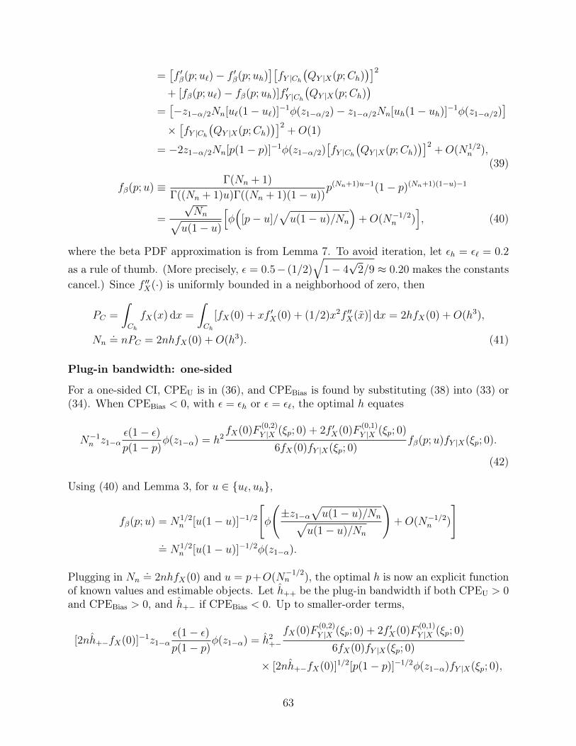
=[f ′β(p;u`)− f ′β(p;uh)
][fY |Ch
(QY |X(p;Ch)
)]2+ [fβ(p;u`)− fβ(p;uh)]f
′Y |Ch
(QY |X(p;Ch)
)=[−z1−α/2Nn[u`(1− u`)]−1φ(z1−α/2)− z1−α/2Nn[uh(1− uh)]−1φ(z1−α/2)
]×[fY |Ch
(QY |X(p;Ch)
)]2+O(1)
= −2z1−α/2Nn[p(1− p)]−1φ(z1−α/2)[fY |Ch
(QY |X(p;Ch)
)]2+O(N1/2
n ),(39)
fβ(p;u) ≡ Γ(Nn + 1)
Γ((Nn + 1)u)Γ((Nn + 1)(1− u))p(Nn+1)u−1(1− p)(Nn+1)(1−u)−1
=
√Nn√
u(1− u)
[φ(
[p− u]/√u(1− u)/Nn
)+O(N−1/2
n )], (40)
where the beta PDF approximation is from Lemma 7. To avoid iteration, let εh = ε` = 0.2
as a rule of thumb. (More precisely, ε = 0.5− (1/2)√
1− 4√
2/9 ≈ 0.20 makes the constantscancel.) Since f ′′X(·) is uniformly bounded in a neighborhood of zero, then
PC =
∫Ch
fX(x) dx =
∫Ch
[fX(0) + xf ′X(0) + (1/2)x2f ′′X(x)] dx = 2hfX(0) +O(h3),
Nn.= nPC = 2nhfX(0) +O(h3). (41)
Plug-in bandwidth: one-sided
For a one-sided CI, CPEU is in (36), and CPEBias is found by substituting (38) into (33) or(34). When CPEBias < 0, with ε = εh or ε = ε`, the optimal h equates
N−1n z1−α
ε(1− ε)p(1− p)
φ(z1−α) = h2fX(0)F
(0,2)Y |X (ξp; 0) + 2f ′X(0)F
(0,1)Y |X (ξp; 0)
6fX(0)fY |X(ξp; 0)fβ(p;u)fY |X(ξp; 0).
(42)
Using (40) and Lemma 3, for u ∈ {u`, uh},
fβ(p;u) = N1/2n [u(1− u)]−1/2
[φ
(±z1−α
√u(1− u)/Nn√
u(1− u)/Nn
)+O(N−1/2
n )
].= N1/2
n [u(1− u)]−1/2φ(z1−α).
Plugging in Nn.= 2nhfX(0) and u = p+O(N
−1/2n ), the optimal h is now an explicit function
of known values and estimable objects. Let h++ be the plug-in bandwidth if both CPEU > 0and CPEBias > 0, and h+− if CPEBias < 0. Up to smaller-order terms,
[2nh+−fX(0)]−1z1−αε(1− ε)p(1− p)
φ(z1−α) = h2+−fX(0)F
(0,2)Y |X (ξp; 0) + 2f ′X(0)F
(0,1)Y |X (ξp; 0)
6fX(0)fY |X(ξp; 0)
× [2nh+−fX(0)]1/2[p(1− p)]−1/2φ(z1−α)fY |X(ξp; 0),
63

and solving for h (and plugging in estimators of the unknown objects) yields the expressionin the text. The extra coefficient on h++ is due to taking the first-order condition of theCPE minimization problem rather than simply setting the two types of CPE to sum to zero.These h hold for both lower and upper one-sided inference.
Plug-in bandwidth: two-sided, p = 1/2
For two-sided inference with p = 1/2, the Bh term becomes zero, as shown in (44). ThenCPEBias < 0 since B2
h > 0, f ′QI,u`Y |Ch
(p) < 0, and f ′QI,uhY |Ch
(p) > 0. The optimal h sets CPEBias +
CPEU.= 0. Substituting (37) and (39) into (35), h solves
N−1n z1−α/2
εh(1− εh) + ε`(1− ε`)p(1− p)
φ(z1−α/2)
= −(1/2)h4
(fX(0)F
(0,2)Y |X (ξp; 0) + 2f ′X(0)F
(0,1)Y |X (ξp; 0)
6fX(0)fY |X(ξp; 0)
)2
×{−z1−α/2Nnφ(z1−α/2)2[p(1− p)]−1
[fY |X(ξp; 0)
]2},
[2nhfX(0)]−22ε(1− ε)
=h4
36fX(0)2fY |X(ξp; 0)
(fX(0)F
(0,2)Y |X (ξp; 0) + 2f ′X(0)F
(0,1)Y |X (ξp; 0)
)2
,
h = n−1/3∣∣∣fX(0)F
(0,2)Y |X (ξp; 0) + 2f ′X(0)F
(0,1)Y |X (ξp; 0)
∣∣∣−1/3
, (43)
again using rule-of-thumb ε = 0.2 and rounding down a leading 1.19 to one.
Plug-in bandwidth: two-sided, p 6= 1/2
For two-sided inference with p 6= 1/2, the dominant bias terms do not cancel completely, butthe difference is of smaller order than the O(N
1/2n ) in the one-sided case. From (46),
fβ(p;uh)− fβ(p;u`) = −(1/3)z1−α/2φ(z1−α/2)2p− 1
p(1− p)+O(N−1/2
n ) = O(1).
Our two CPE terms are thus of orders N−1n � n−1h−1 and h2. This implies that h∗ � n−1/3
and that CPE is O(n−2/3). If so, the B2h term is of order h4Nn = h5n = n−2/3, so it must
also be included. Although the second term from the product rule derivative in the B2h term
is not zero this time, it is smaller-order and thus omitted below.Using (35), (38), (39), and (46),
CPEBias.= Bh
[fQI,uhY |Ch
(QY |X(p;Ch)
)− f
QI,u`Y |Ch
(QY |X(p;Ch)
)]+ (1/2)B2
h
[f ′QI,u`Y |Ch
(QY |X(p;Ch)
)− f ′
QI,u`Y |Ch
(QY |X(p;Ch)
)]
64

.= BhfY |Ch
(F−1Y |Ch(p)
)[fβ(p;uh)− fβ(p;u`)]
− (1/2)B2hz1−α/2Nnφ(z1−α/2)2[p(1− p)]−1
[fY |Ch
(F−1Y |Ch(p)
)]2
.=fY |X(ξp; 0)z1−α/2φ(z1−α/2)
p(1− p)[Bh(1− 2p)/3−B2
hNnfY |X(ξp; 0)]. (44)
With large enough h, (44) is always negative, so there always exists an optimal h that cancelsthe dominant terms of CPEU and CPEBias. This h solves
−N−1n z1−α/2
εh(1− εh) + ε`(1− ε`)p(1− p)
φ(z1−α/2)
=fY |X(ξp; 0)z1−α/2φ(z1−α/2)
p(1− p)[Bh(1− 2p)/3−B2
hNnfY |X(ξp; 0)].
Continuing to solve for h using (41) and then Lemma 5,
−[2nhfX(0)]−12ε(1− ε)
= fY |X(ξp; 0){h2(Bh/h
2)(1− 2p)/3− h4(B2h/h
4)[2nhfX(0)]fY |X(ξp; 0)},{
n−1[fX(0)]−1ε(1− ε)}
= h6{
2n[fY |X(ξp; 0)
]2fX(0)B2
h/h4}− h3
{fY |X(ξp; 0)[(1− 2p)/3]Bh/h
2},
0 = (h3)2{na} − (h3){b} − {c/n},
h3 =b±√b2 + 4ac
2an,
h = n−1/3
(Bh/|Bh|)(1− 2p) +√
(1− 2p)2 + 4
2∣∣∣fX(0)F
(0,2)Y |X (ξp; 0) + 2f ′X(0)F
(0,1)Y |X (ξp; 0)
∣∣∣1/3
,
setting ε to match (43) when p = 1/2.
Plug-in bandwidth: beta PDF difference approximation
The following approximates the beta PDF difference fβ(p;uh)− fβ(p;u`). For either u = uhor u = u`, from the proof of Lemma 7, where here ∆x1 = p, ∆x2 = 1− p, ∆k1 = (n + 1)u,∆k2 = (n+ 1)(1− u), J = 1, and u− p = O(n−1/2),
log(f∆X(∆x)) = K + h(∆x) +O(n−1),
K = (J/2) log(n/2π) +1
2
J+1∑j=1
log(n/[∆kj − 1]),
eK =[1 +O(n−1)
]√ n
2π
√1
u(1− u),
65

h(∆x) = −(1/2)(n− J)2
J+1∑j=1
(∆xj − [∆kj − 1]/[n− J ])2
∆kj − 1
+ (1/3)(n− J)3
J+1∑j=1
(∆xj − [∆kj − 1]/[n− J ])3
(∆kj − 1)2+O(n−1)
= −(1/2)n[(u− p)2/[u(1− u)] + 2(u− p)(2u− 1)/[nu(1− u)]
](45)
+ (1/3)n(p− u)3[u−2 − (1− u)−2] +O(n−1).
First, note that eK will put the√n coefficient in front, so the O(n−1) remainder in
h(∆x) is required in order to yield O(n−1/2) overall. Even within eK , we must keep track ofu = p± n−1/2z
√p(1− p) +O(n−1), not just u ≈ p, where for brevity z ≡ z1−α/2. So
[uh(1− uh)]−1/2 = [p(1− p)]−1/2 − (1/2)n−1/2z1− 2p
p(1− p)+O(n−1),
eK(uh) =n1/2√
2πp(1− p)
[1 + (1/2)n−1/2z
2p− 1√p(1− p)
]+O(n−1/2),
eK(u`) =n1/2√
2πp(1− p)
[1− (1/2)n−1/2z
2p− 1√p(1− p)
]+O(n−1/2).
Second, for uh, let uh = p+n−1/2c1 +n−1c2 +O(n−3/2) from Lemma 3. Then, (u− p)2 =n−1c2
1 + 2n−3/2c1c2 +O(n−2) and (u− p)3 = n−3/2c31 +O(n−2). Plugging into (45) and using
the small x approximations ex = 1 + x+O(x2) and 1/(1 + x) = 1− x+O(x2),
h(∆x) = −1
2
c21
p(1− p)− n−1/2
(c1(c2 + 2p− 1)
p(1− p)− (2p− 1)c3
1
3p2(1− p)2+
c21z(2p− 1)
2[p(1− p)]3/2
)+O(n−1)
= −z2/2− 2n−1/2z2p− 1
3√p(1− p)
+O(n−1),
exp{h(∆x)} = e−z2/2
[1− (2/3)n−1/2z
2p− 1√p(1− p)
]+O(n−1),
while for u`,
exp{h(∆x)} = e−z2/2
[1 + (2/3)n−1/2z
2p− 1√p(1− p)
]+O(n−1).
Altogether,
fβ(p;uh) =n1/2√p(1− p)
φ(z)
[1− (1/6)n−1/2z
2p− 1√p(1− p)
]+O(n−1/2),
fβ(p;u`) =n1/2√p(1− p)
φ(z)
[1 + (1/6)n−1/2z
2p− 1√p(1− p)
]+O(n−1/2),
66

fβ(p;uh)− fβ(p;u`) = −(1/3)zφ(z)2p− 1
p(1− p)+O(n−1/2). (46)
67
![arXiv:1703.05813v2 [math.GT] 16 May 2018 · bracket. For all expansions θwe have {−,−}θ = {−,−}KKS + higher order terms. It turns out that there is a class of expansions,](https://img.dokumen.tips/doc/110x75/5dd0cbfcd6be591ccb62be26/arxiv170305813v2-mathgt-16-may-2018-bracket-for-all-expansions-we-have-aa.jpg)