Fractals don’t have to be scary. Mandelbrot Maps: … · \Fractals don’t have to be scary." Mandelbrot Maps: Creating a real-time Mandelbrot/Julia fractal explorer Iain Parris

$Page 1: Fractals don’t have to be scary. Mandelbrot Maps: … · \Fractals don’t have to be scary." Mandelbrot Maps: Creating a real-time Mandelbrot/Julia fractal explorer Iain Parris$
“Fractals don’t have to be scary.”

Mandelbrot Maps : Creating a real-time

Mandelbrot/Julia fractal explorer

Iain Parris

DissertationMSc in Computer Science

School of InformaticsUniversity of Edinburgh

22 August 2008

1

Abstract

Mandelbrot Maps is a new fractal explorer applet, capable of providingreal-time exploration of the Mandelbrot set and associated Julia sets –with an emphasis on allowing intuitive exploration.

The user interface is designed to be natural, easy-to-use, and unobtru-sive. Furthermore, real-time interaction is found to be both achievable,and desirable.

The overall result is a fractal explorer intended to be interesting, ac-cessible, and fun for people with a wide range of previous mathematicalor computer exposure – from the layman to the expert.

2

AcknowledgementsWith thanks to:

Philip Wadler My supervisor for this project, who has offered invaluable ad-vice and direction.

Douglas Armstrong For some dissertation write-up pointers.

My parents For the food, place to live, and remarkably good imitation of theaverage computer user – particularly useful when needing feedback fromreal people.

My friends For keeping me sane.

Brandilynn French Last but not least, my fiancee, Brandi. For everything.I dedicate this dissertation to you.

3

DeclarationI declare that this thesis was composed by myself, that the work containedherein is my own except where explicitly stated otherwise in the text, and thatthis work has not been submitted for any other degree of professional qualifica-tion except as specified.

(Iain Parris)

4

Contents

1 Introduction 6

2 Mathematical Background 102.1 Mandelbrot Set . . . . . . . . . . . . . . . . . . . . . . . . . . . . 10

2.1.1 Definition . . . . . . . . . . . . . . . . . . . . . . . . . . . 102.1.2 Escape-time Algorithm . . . . . . . . . . . . . . . . . . . 112.1.3 Visualising the Mandelbrot set . . . . . . . . . . . . . . . 12

2.2 Julia Sets . . . . . . . . . . . . . . . . . . . . . . . . . . . . . . . 122.3 Connectedness of a Julia set . . . . . . . . . . . . . . . . . . . . . 142.4 Other Mathematical Results . . . . . . . . . . . . . . . . . . . . . 14

3 Pre-existing Fractal Explorers 163.1 Applet: by James Henstridge . . . . . . . . . . . . . . . . . . . . 16

3.1.1 Description . . . . . . . . . . . . . . . . . . . . . . . . . . 163.1.2 Critical Review . . . . . . . . . . . . . . . . . . . . . . . . 17

3.2 Applet: by Alexander Bogomolny . . . . . . . . . . . . . . . . . . 183.2.1 Description . . . . . . . . . . . . . . . . . . . . . . . . . . 183.2.2 Critical Review . . . . . . . . . . . . . . . . . . . . . . . . 19

3.3 Applet: The Quadratic Map, by Yakov Shapiro . . . . . . . . . . 203.3.1 Description . . . . . . . . . . . . . . . . . . . . . . . . . . 203.3.2 Critical Review . . . . . . . . . . . . . . . . . . . . . . . . 21

3.4 Applet: Julia Animator, by Evgeny Demidov . . . . . . . . . . . 223.4.1 Description . . . . . . . . . . . . . . . . . . . . . . . . . . 223.4.2 Critical Review . . . . . . . . . . . . . . . . . . . . . . . . 23

4 Design and Implementation of Mandelbrot Maps 244.1 Initial Design . . . . . . . . . . . . . . . . . . . . . . . . . . . . . 24

4.1.1 Overall Architecture . . . . . . . . . . . . . . . . . . . . . 254.1.2 Creating a Prototype . . . . . . . . . . . . . . . . . . . . . 254.1.3 Lessons from the Prototype . . . . . . . . . . . . . . . . . 26

4.2 Zooming . . . . . . . . . . . . . . . . . . . . . . . . . . . . . . . . 264.2.1 How to zoom? . . . . . . . . . . . . . . . . . . . . . . . . 274.2.2 Implementing Mouse Wheel Zooming . . . . . . . . . . . 284.2.3 Zoom Limits . . . . . . . . . . . . . . . . . . . . . . . . . 28

4.3 Zoom Slider . . . . . . . . . . . . . . . . . . . . . . . . . . . . . . 294.4 Panning (moving around the canvas) . . . . . . . . . . . . . . . . 294.5 Home Button . . . . . . . . . . . . . . . . . . . . . . . . . . . . . 294.6 Save . . . . . . . . . . . . . . . . . . . . . . . . . . . . . . . . . . 29

4.6.1 Variety of Resolutions . . . . . . . . . . . . . . . . . . . . 304.7 Bookmarking: Show URL . . . . . . . . . . . . . . . . . . . . . . 314.8 Colouring the Image . . . . . . . . . . . . . . . . . . . . . . . . . 324.9 Number of Iterations to Perform . . . . . . . . . . . . . . . . . . 36

4.9.1 Quantifying the Iteration Upper Bound . . . . . . . . . . 394.9.2 Contrast Slider . . . . . . . . . . . . . . . . . . . . . . . . 41

5

4.10 Rendering . . . . . . . . . . . . . . . . . . . . . . . . . . . . . . . 414.10.1 Efficient Painting . . . . . . . . . . . . . . . . . . . . . . . 414.10.2 “Blocky Squares” Crude-first Rendering . . . . . . . . . . 424.10.3 Rendering Threads . . . . . . . . . . . . . . . . . . . . . . 42

5 User Evaluation 445.1 Method . . . . . . . . . . . . . . . . . . . . . . . . . . . . . . . . 44

5.1.1 Real-time Tickbox Features . . . . . . . . . . . . . . . . . 445.1.2 Why the two modes? . . . . . . . . . . . . . . . . . . . . . 455.1.3 Survey . . . . . . . . . . . . . . . . . . . . . . . . . . . . . 455.1.4 Advertising the survey . . . . . . . . . . . . . . . . . . . . 46

5.2 User Feedback . . . . . . . . . . . . . . . . . . . . . . . . . . . . 475.2.1 User Base . . . . . . . . . . . . . . . . . . . . . . . . . . . 475.2.2 Features Understood . . . . . . . . . . . . . . . . . . . . . 475.2.3 Comments . . . . . . . . . . . . . . . . . . . . . . . . . . . 485.2.4 Image Quality . . . . . . . . . . . . . . . . . . . . . . . . 495.2.5 Bugs Fixed . . . . . . . . . . . . . . . . . . . . . . . . . . 50

5.3 Testing the Real-time Hypothesis . . . . . . . . . . . . . . . . . . 51

6 Future Work 546.1 Rendering Rate . . . . . . . . . . . . . . . . . . . . . . . . . . . . 54

6.1.1 Multicore . . . . . . . . . . . . . . . . . . . . . . . . . . . 546.1.2 Panning – with cached rendering . . . . . . . . . . . . . . 556.1.3 Re-use work from the crude renderings . . . . . . . . . . . 55

6.2 Colour Schemes . . . . . . . . . . . . . . . . . . . . . . . . . . . . 556.3 Deep Zoom . . . . . . . . . . . . . . . . . . . . . . . . . . . . . . 556.4 Beyond Quadratics . . . . . . . . . . . . . . . . . . . . . . . . . . 56

7 Conclusion 56

References 56

1 Introduction

The new Java applet written for this MSc project, Mandelbrot Maps – and aquick-start video guide to the applet for an end user – are available online athttp://homepages.inf.ed.ac.uk/s0790125/mmaps/

Background The Mandelbrot set, and associated Julia sets, are examples offractals – shapes where self-similarity may be observed on all scales[10]. How-ever, this extraordinary complexity all arises from one extremely-simple equa-tion1

1The equation behind these fractal images is: zn+1 = z2n + c. For further details, see

Section 2.

6

http://homepages.inf.ed.ac.uk/s0790125/mmaps/

There is only one Mandelbrot set – which is fundamentally just a set ofpoints lying on the complex plane. The Mandelbrot set is named in honour ofthe mathematician Benoıt Mandelbrot, for his work in the 1980s.

While there is only one Mandelbrot set, there are numerous Julia sets, eachone also lying on the complex plane. There is a Julia set corresponding toevery single point in the complex plane; that is, each point in the complex planeparameterizes a Julia set. So, if a particular point on the complex plane ischosen, a Julia set corresponding to this point (parameterized by it) may bedrawn onto the complex plane. Julia sets are named for Gaston Julia, for hiswork on complex dynamics in the 1900s.

The Mandelbrot set and the Julia sets are closely related. Indeed, thereare a number of remarkable results about the Mandelbrot set, and associatedJulia sets. These results are typically expressed only in abstruse mathematicallanguage, and are therefore completely inaccessible to all but a tiny minority ofpeople.

Fractal explorers present an image of the Mandelbrot set, and allow selection(in some way) of a point on this image. The Julia set parameterized by this pointwill subsequently be generated and displayed. This process may be repeated,to generate numerous Julia sets parameterized by different points.

One interesting result is that there are often striking resemblances betweenthe Mandelbrot set in the region of the point selected, and the associated Juliaset. For two examples of this phenomenon of quasi-similarity, see Figures 1 and2.

Existing Explorers Because typical modern desktop computers are able topresent fairly rapid visualisations of the Mandelbrot set and Julia sets, therealready exist numerous other explorers on the web2, normally presented as Javaapplets. These explorers aim to aid human intuition of these mathematicalconstructs.

The subset of previously-existing explorers which I have been able to examineall have (in my personal opinion) considerable room for improvement in theiruser interfaces, which are ugly and unintuitive – to the point of limiting theinsight into the mathematical results that may be easily obtained by use of eachexplorer, and making the explorers inaccessible to many people.

Mandelbrot Maps Project The overall goal of this project has been todevelop a new program for intuitive exploration of the Mandelbrot set, andassociated Julia sets. This explorer is free and open source software, and isintended to be suitable for use in education.

The key innovation of Mandelbrot Maps is in allowing real-time interaction.Rendering fractal images is computationally expensive. This therefore requiredcareful engineering to improve the response time – for example, by means ofdrawing a fast crude rendering first, followed by filling in the details later, when

2A Google search for Mandelbrot Julia Program yields over 50,000 hits – as of August2008. Only a small subset of these have been surveyed.

7

Figure 1: Example of quasi-similarity: resemblance between a region of theMandelbrot set (top) and a Julia set parameterized by a point within this region(bottom) – images generated by Mandelbrot Maps.

8

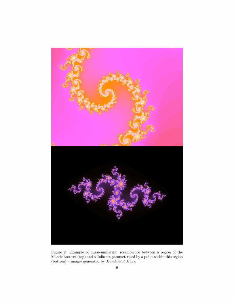
Figure 2: Example of quasi-similarity: resemblance between a region of theMandelbrot set (top) and a Julia set parameterized by a point within this region(bottom) – images generated by Mandelbrot Maps.

9

appropriate. This is coupled with the results of a user survey, which indicatethat users do indeed show a preference for real-time interaction.

Other innovations include:

• Careful attention to the user interface. Where appropriate, similarities tothe popular and generally-familiar Google Maps interface[2] are exploited– hence the name of this applet, Mandelbrot Maps.

• Colouring the generated images in an aesthetically-pleasing way.

• Automating the setting of the upper bound of iterations that will be per-formed by the applet using the escape time algorithm, to make this taskas transparent to the user as possible. (For an explanation of this jargon,see sections 2.1.2 and 4.9.) Setting a good upper bound is very desirable:too high an upper bound results in doing too much work and thereforeslows image generation; too low an upper bound results in inaccurate andmisleading images being shown.

The end result is an applet designed to be interesting, usable and fun for avery broad range of people, with a wide range of pre-existing mathematical orcomputer knowledge – from the layman to the expert.

2 Mathematical Background

Detailed mathematical background, and formal proofs, are out of scope for thisdissertation. However, some general background and results are described inthis section.

2.1 Mandelbrot Set

Most of the information for this section, and section 2.2, is summarised basedon [4].

2.1.1 Definition

Let f(z) = z2 + c. We may iterate this complex function.That is, given zn:

zn+1 = f(zn) = z2n + c

So, setting z0 = 0, we may enumerate the first few iterations:

z0 = 0

z1 = f(z0) = z20 + c = c

z2 = f(z1) = z21 + c = c2 + c

z3 = f(z2) = z22 + c = (c2 + c)2 + c

10

The orbit of 0 is the collection of all of these points z0, z1, z2, ...So, for our f(z) = z2 + c, the orbit of 0 is: 0, c, c2 + c, ...The fate of the orbit of 0 is the eventual behaviour of the orbit of 0. There

are various possible fates, depending – for our particular f(z) – only on thevalue of c. The fate may be:

• Tending towards, or reaching, a fixed point

• Tending towards, or entering, a cycle of some period

• Chaotically bouncing around without divergence

• Diverging to infinity (ie, The orbit of 0 escapes)

The Mandelbrot set may be defined as all the points c in the complex plane forwhich the orbit of 0 remains bounded – that is, does not escape (tend towardsinfinity) – under iteration of f(z) = z2 + c.

2.1.2 Escape-time Algorithm

There is a well-known result3 that if some |zn| > 2, the overall fate is to tendtowards infinity. This leads to a way to test if a point c is within the Mandelbrotset: follow the orbit of 0 for this c for some number of iterations. If we ever seethe orbit of 0 stray outside the circle centred on the origin with radius 2 (ie,some |zn| > 2), then we know that this c is definitely not within the Mandelbrotset, and can stop iterating.

Note that we must define some upper bound on the number of iterationswe will trace, in case we get stuck tending towards a cycle or a fixed point –in which case, with no upper bound, this algorithm would not terminate. Ifthe maximum number of iterations is reached, we therefore assume the point iswithin the Mandelbrot set.

With this algorithm, a point within the Mandelbrot set is never miscate-gorised as not within the Mandelbrot set, but some points outside the Mandel-brot set may be miscategorised as within the Mandelbrot set (if the maximumnumber of iterations is performed without seeing divergence, but the orbit wouldhave eventually diverged later). The higher this upper bound on the number ofiterations, the lower the likelihood of mistakenly categorising a slow-to-divergepoint as within the Mandelbrot set.

With a computer, we may draw an approximation to the Mandelbrot set bytesting many points c within a portion of the complex plane, and colouring themaccording to whether or not they are in the Mandelbrot set. While, with thisalgorithm, only one colour may be assigned to points within the Mandelbrotset (or more accurately, assumed to be within the Mandelbrot set as we havehit the maximum iterations limit), we may choose different colours for pointsoutside the Mandelbrot set, depending on how many iterations were requiredto determine that the point is definitely outwith the Mandelbrot set – that is,

3A formal proof is out of scope for this dissertation.

11

Figure 3: The Mandelbrot Set

until we first find some |zn| > 2. This colour may be interpreted as the point’s“distance” from the Mandelbrot set.

2.1.3 Visualising the Mandelbrot set

Figure 3 shows an image of the Mandelbrot set, created using the escape-timealgorithm with a simple colouring algorithm: greyscale image, with point inten-sities proportional to the number of iterations calculated for that point.

Looking at the overall structure of the Mandelbrot set, we can see thatthere is a large main cardioid in the centre of the Mandelbrot set. There areinfinitely-many smaller bulbs (primary bulbs) attached to this main cardioid.

2.2 Julia Sets

There is only one Mandelbrot set. There is a Julia set for every point in thecomplex plane; each Julia set has a complex parameter c.

Given some complex point c, the filled Julia set parameterized by this c isthe set of points z in the complex plane for which the orbit of z (ie, z0 = z)under iteration of zn+1 = f(zn) = z2

n + c remains bounded.Enumerating the first few iterations:

12

Figure 4: A Julia set

z0 = z

z1 = z20 + c = z2 + c

z2 = z21 + c = (z2 + c)2 + c

If the series of zs does not diverge, z0 = z is in the filled Julia set pa-rameterized by c. The Julia set is the boundary of the associated filled Juliaset.

Using the same escape-time algorithm (with trivial modification) describedin 2.1.2 for drawing the Mandelbrot set, we may draw different filled Julia sets.Figure 4 shows one filled Julia set generated in such a way, again with the simplegreyscale colouring.

13

2.3 Connectedness of a Julia set

Fundamental Dichotomy[18] The fundamental dichotomy for z2 +c is thatevery filled Julia set is either totally connected (it is just “one piece”), or totallydisconnected (a Cantor set, or fractal dust). A Cantor set has no two pointstouching, but yet infinitely many other points scattered within any non-zeroradius disc around any point. Loosely, a Cantor set may be visualised as adense “cloud” of disconnected points.

Mandelbrot set as an index of Julia sets Even more remarkable is thatwe can find whether a given Julia set is a connected set or a Cantor set byexamination of the Mandelbrot set. If the complex number c parameterizingthe given Julia set is within the Mandelbrot set, the Julia set is connected.Otherwise, the Julia set is a Cantor set.[18]

2.4 Other Mathematical Results

There are numerous other results, beyond the few described above. An excel-lent summary of some of these results has been compiled by Devaney, in [11].Detailed description – let alone proof – of these results is out of scope for thisdocument, but this is a short summary of some of the more notable results:

Shattering[13] As c parameterizing the Julia sets leaves the Mandelbrot set,the filled Julia sets shatter – from totally connected sets to Cantor sets,as the boundary of the Mandelbrot set is crossed.

Bifurcations[14] As c parameterizing the Julia sets moves from the Mandel-brot set’s main cardioid, into the primary bulbs, the associated filled Juilasets “pinch” together: this type of change is known as a bifurcation.

Periods of the Primary Bulbs[15][19][20] As described in 2.1, each bulbhas an associated period. There are two geometric results relating to theperiods of these bulbs:

Mandelbrot Set Geometry[20] Spokes (antennae) emanate from thebulbs of the Mandelbrot set. The number of spokes in the largestantenna attached to a primary bulb is the period of the bulb.

Julia Set Geometry[19] For filled Julia sets parameterized by c withinthe primary bulbs of the Mandelbrot set, the period of the primarybulb can be read off from the filled Julia set’s structure: there exist(an infinite number of) junction points where n “segments” of thefilled Julia set are joined by only a single point. n is the period ofthe primary bulb.

Rotation Numbers of the Primary Bulbs[16][17][19] Primary bulbs havean associated rotation number (definitions in [16], [17] and [19]). There isa relationship between the rotation number and:

14

• The angle the primary bulb makes with the main cardioid of theMandelbrot set

• The geometry of the associated Julia sets – ie, those parameterizedby c within the given primary bulb

• The geometry of the Mandelbrot set near the primary bulb

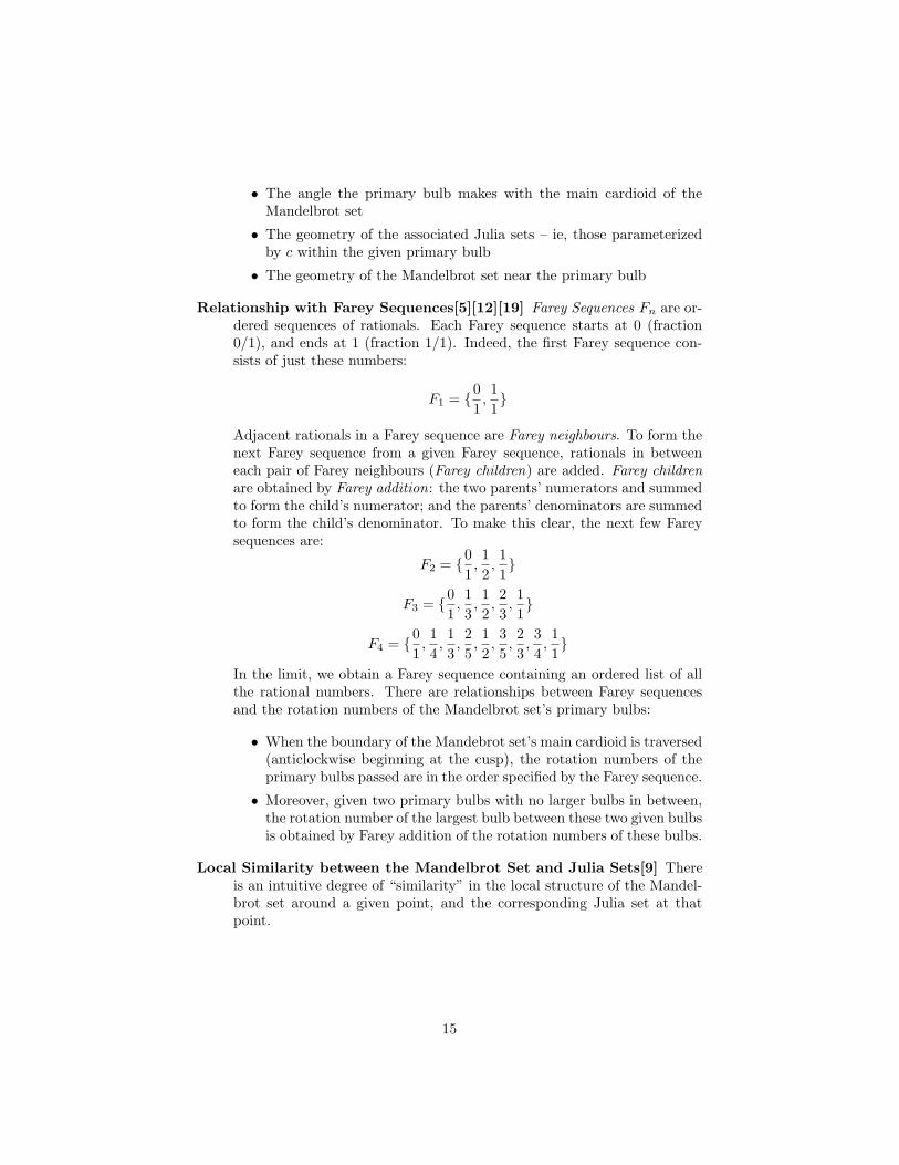
Relationship with Farey Sequences[5][12][19] Farey Sequences Fn are or-dered sequences of rationals. Each Farey sequence starts at 0 (fraction0/1), and ends at 1 (fraction 1/1). Indeed, the first Farey sequence con-sists of just these numbers:

F1 = {01,

11}

Adjacent rationals in a Farey sequence are Farey neighbours. To form thenext Farey sequence from a given Farey sequence, rationals in betweeneach pair of Farey neighbours (Farey children) are added. Farey childrenare obtained by Farey addition: the two parents’ numerators and summedto form the child’s numerator; and the parents’ denominators are summedto form the child’s denominator. To make this clear, the next few Fareysequences are:

F2 = {01,

12,

11}

F3 = {01,

13,

12,

23,

11}

F4 = {01,

14,

13,

25,

12,

35,

23,

34,

11}

In the limit, we obtain a Farey sequence containing an ordered list of allthe rational numbers. There are relationships between Farey sequencesand the rotation numbers of the Mandelbrot set’s primary bulbs:

• When the boundary of the Mandebrot set’s main cardioid is traversed(anticlockwise beginning at the cusp), the rotation numbers of theprimary bulbs passed are in the order specified by the Farey sequence.

• Moreover, given two primary bulbs with no larger bulbs in between,the rotation number of the largest bulb between these two given bulbsis obtained by Farey addition of the rotation numbers of these bulbs.

Local Similarity between the Mandelbrot Set and Julia Sets[9] Thereis an intuitive degree of “similarity” in the local structure of the Mandel-brot set around a given point, and the corresponding Julia set at thatpoint.

15

Figure 5: Screenshot of James Henstridge’s applet

3 Pre-existing Fractal Explorers

There are numerous pre-existing Mandelbrot/Julia explorers; a Google searchyields over 6,000 hits for Mandelbrot Julia Explorer, as of August 2008. It isinfeasible to survey and critique them all. Therefore, I present here four of thebest applets which I could find after viewing the webpages found in the firstfew pages of Google results (and following some of the links contained thereinto other webpages and applets), along with critical review of these applets.

3.1 Applet: by James Henstridge

The first applet reviewed is by James Henstridge. It is available online at [7].Figure 5 shows a screenshot of its default start screen.

3.1.1 Description

This applet has a single pane, used at any one time to display either the Man-delbrot set or a Julia set.

16

The 5 on the default start screen is part of a dropdown box, with options:n = {1, 2, 5, 10}. Changing this option (and clicking Redraw) adjusts the “block-iness” of the images generated. Instead of calculating the time to escape at everypixel, each point computed is scaled up to n×n pixels in the final image – lead-ing to the creation of an image with n × n times fewer pixels. For instance,setting n = 5 means generating an image of 5 × 5 = 25 times fewer pixels.Presumably, this is done for efficiency: a user of a slower computer may accepta more “blocky” image, because it may be generated approximately n×n timesfaster (assuming each point takes roughly the same amount of time to compute).

Clicking Zoom In allows the user to draw a selection box with the mouse.The view then updates, to show only the contents of the selection box – scaledup to fill the viewing area.

Switch (M <-> J) is used to toggle between showing the Mandelbrot set,or a Julia set. Pressing this button, then clicking a point on the Mandelbrotset causes the window to refresh, showing the Julia set of complex parametercorresponding to the point clicked. Clicking the button again returns to thedisplay of the Mandelbrot set.

3.1.2 Critical Review

Low-quality rendering option A user with a slower computer may chooseto have a lower-quality image generated, in a shorter amount of time. If theylike the image shown, and want to see more detail, they must manually choosethe higher-quality setting, and redraw. This is perhaps a disadvantage – oncethe low-quality image is generated and displayed, why not automatically startgenerating the higher-quality image, in case the user is prepared to wait to seesome more detail?

Seeing Julia sets The correspondence between the Mandelbrot set and theJulia sets is made quite clear, by explicitly allowing a click within the Mandel-brot set (after first priming the applet with the Switch button) to generate thecorresponding Julia set.

However, the modal interface, which allows displaying either a Mandelbrotset or a Julia set but not both, is a bit cumbersome. What if we wanted to see afew Julia sets in close proximity? We would have to generate them one-by-one,by: remembering the complex parameter for the Julia set; changing modes backto show the Mandelbrot set; clicking another point on the Mandelbrot set nearthe original point we chose; etc.

Zooming Zooming is fairly simple to understand – a selection box is a familiarconcept.

However, there are some inherent problems:

• The selection box is unconstrained – allowed to be any shape of rectangle.The user may thus easily create a selection with a different aspect ratio tothe viewing area. When the viewing area is updated, a distorted, stretched

17

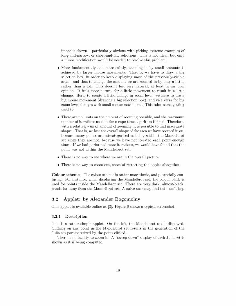
image is shown – particularly obvious with picking extreme examples oflong-and-narrow, or short-and-fat, selections. This is not ideal, but onlya minor modification would be needed to resolve this problem.

• More fundamentally and more subtly, zooming in by small amounts isachieved by larger mouse movements. That is, we have to draw a bigselection box, in order to keep displaying most of the previously-visiblearea – and thus to change the amount we are zoomed in by only a little,rather than a lot. This doesn’t feel very natural, at least in my ownopinion. It feels more natural for a little movement to result in a littlechange. Here, to create a little change in zoom level, we have to use abig mouse movement (drawing a big selection box); and vice versa for bigzoom level changes with small mouse movements. This takes some gettingused to.

• There are no limits on the amount of zooming possible, and the maximumnumber of iterations used in the escape-time algorithm is fixed. Therefore,with a relatively-small amount of zooming, it is possible to find inaccurateshapes. That is, we lose the overall shape of the area we have zoomed in on,because many points are miscategorised as being within the Mandelbrotset when they are not, because we have not iterated each point enoughtimes. If we had performed more iterations, we would have found that thepoint was not within the Mandelbrot set.

• There is no way to see where we are in the overall picture.

• There is no way to zoom out, short of restarting the applet altogether.

Colour scheme The colour scheme is rather unaesthetic, and potentially con-fusing. For instance, when displaying the Mandelbrot set, the colour black isused for points inside the Mandelbrot set. There are very dark, almost-black,bands far away from the Mandelbrot set. A naıve user may find this confusing.

3.2 Applet: by Alexander Bogomolny

This applet is available online at [3]. Figure 6 shows a typical screenshot.

3.2.1 Description

This is a rather simple applet. On the left, the Mandelbrot set is displayed.Clicking on any point in the Mandelbrot set results in the generation of theJulia set parameterized by the point clicked.

There is no facility to zoom in. A “sweep-down” display of each Julia set isshown as it is being computed.

18

Figure 6: Screenshot of Alexander Bogomolny’s applet


Simplicity The applet’s simplicity makes it easy to use, and to understand.Having both the Mandelbrot set and the latest-generated Julia set on screen

at the same time is a natural arrangement. Toggling between different modesand views, as was the case in Henstridge’s applet, is cumbersome; displayingeverything on screen at once is a more elegant solution.

Clicking the Mandelbrot set allows the generation of a Julia set. This makesit easy to generate “nearby” Julia sets – just click, wait for it to be generated,move the mouse slightly, and click again at a point nearby.

Low Resolution Unfortunately, the images generated with the applet arevery small (ie, few pixels). There is no way to increase the resolution of theseimages.

Colour Scheme The Mandelbrot set’s colouring is OK, if not very aesthetically-pleasing. But, as shown in the screenshot in Figure 6, the Julia sets’ colours aredark, and jarring. The image has aliases introduced by the colouring scheme: agrainy appearance.

Rendering Speed With a fairly fast CPU (by 2008 standards; an E6750Intel Core 2 Duo CPU @ 2.66Ghz), it takes ˜2 seconds to generate each Juliaset image. This feels slow.

Missing Features The applet is most limited by its missing features. Inparticular, the lack of a zoom ability.

For gaining an overall feeling of how the Julia sets vary at points across theun-zoomed-in Mandelbrot set, though, it is simple and effective.

19

Figure 7: Screenshot of The Quadratic Map, by Yakov Shapiro

3.3 Applet: The Quadratic Map, by Yakov Shapiro

The Quadratic Map was created by Yakov Shapiro. It is available online at [21].Figure 7 shows a screenshot.

Like many – indeed possibly most – of the existing fractal explorers, TheQuadratic Map is powerful, and with good features, but intimidating and noteasy-to-use.

3.3.1 Description

The Quadratic Map has the following main features:

• Generating a Julia set at a given point

– Click a point in the Mandelbrot set

– Click Compute

• Zooming in on arbitrary sections of the Mandelbrot set, or of a generatedJulia set

– Click-and-drag the mouse to create a selection rectangle

– Click Compute

• Viewing the orbit of a point in the Julia set

– Click a point in the Julia set

– Click View orbit (to view the first ten iterations), or Iterate to stepthrough iterations one-by-one

20

• Animating Julia sets, along a path (arbitrary points connected by straightlines) through the Mandelbrot set

– For an arbitrary number of points in the Mandelbrot set,∗ Click the point in the Mandelbrot set∗ Click Add current E

– Click Animate

Additionally, the maximum number of iterations to perform may be set inde-pendently, for the Mandelbrot set or the Julia set. This is useful when zoomingin – when performing more iterations is necessary, to obtain a more accurateimage.


Complicated interface The interface takes some getting used to. Indeed,without reading instructions, a person is unlikely to be able to make muchheadway at all with the applet!

Animation Once mastered, though, animations are quite a nice way of seeinghow the Julia sets vary as their parameterizing complex number varies smoothly,across a portion of the Mandelbrot set.

Unfortunately, there is no indicator of how far along the path we are, whilethe Julia sets are being displayed in sequence, which makes it somewhat trickyto see positions where interesting things happen along a path. For instance,there is no obvious indicator of at when we first see a Julia set correspondingto a point outside the Mandelbrot set, if moving along a path from inside tooutside the Mandelbrot set.

Unconstrained selection box Just as for Henstridge’s applet, the selectionbox used to zoom has some flaws (see Section 3.1.2) – except that now, we cantweak the maximum number of iterations, and thus can have a much less limitedzoom.

Briefly recapping the flaws in common though, which are inherent to usingan (unconstrained) selection box to zoom:

• Unconstrained selection boxes mean that images may be stretched, anddistorted, if the selection rectangle has a different width:height ratio tothe viewing area.

• Zooming feels unnatural – small mouse movements cause large zoom changes,and vice versa.

• There is no indicator of how far we are zoomed in.

• There is no way to zoom out. (Except, possibly, there may be some limitedsuccess with dragging one corner of the selection box outside the appletwindow.)

21

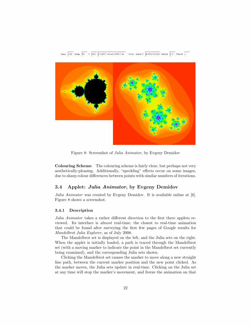
Figure 8: Screenshot of Julia Animator, by Evgeny Demidov

Colouring Scheme The colouring scheme is fairly clear, but perhaps not veryaesthetically-pleasing. Additionally, “speckling” effects occur on some images,due to sharp colour differences between points with similar numbers of iterations.

3.4 Applet: Julia Animator, by Evgeny Demidov

Julia Animator was created by Evgeny Demidov. It is available online at [6].Figure 8 shows a screenshot.

3.4.1 Description

Julia Animator takes a rather different direction to the first three applets re-viewed. Its interface is almost real-time; the closest to real-time animationthat could be found after surveying the first few pages of Google results forMandelbrot Julia Explorer, as of July 2008.

The Mandelbrot set is displayed on the left, and the Julia sets on the right.When the applet is initially loaded, a path is traced through the Mandelbrotset (with a moving marker to indicate the point in the Mandelbrot set currentlybeing examined), and the corresponding Julia sets shown.

Clicking the Mandelbrot set causes the marker to move along a new straightline path, between the current marker position and the new point clicked. Asthe marker moves, the Julia sets update in real-time. Clicking on the Julia setat any time will stop the marker’s movement, and freeze the animation on that

22

particular Julia set.Zooming is possible, centred on a point:

• Zoom in: Alt + Mouse-click

• Zoom out: Ctrl + Mouse-click

Finally, manually adjustments are possible to parameters labelled towards thetop of the applet:

• Steps: How many steps the marker will take along each straight-line path.(For instance, with a value of 100, the marker will take 100 steps alongeach straight line path, to compute 100 Julia sets along this path.)

• Delay : An extra delay between steps.

• It : The upper bound on the maximum number of iterations for the escape-time algorithm.


Real-time animation The near real-time interaction is fairly pleasant. Itis possible to easily create animated progressions of Julia sets along a path,with far less effort than with The Quadratic Map. Just clicking points on theMandelbrot set is all that is now required, in order to animate Julia set changesalong a straight-line path on the Mandelbrot set.

The main inherent shortcoming of this approach is that, if the delay is fairlysmall, it can be hard to keep track of the movement of the marker on theMandelbrot set, while simultaneously watching the changes in the Julia sets.

Unfortunately, there is an additional implementation-specific shortcoming.It is not possible to display an animated magnified region of the Julia sets, asthe marker moves across the Mandelbrot set. It is only possible with this appletto zoom in on sections of a frozen Julia set. As soon as animation begins again,the zoom is lost, and only the overall Julia sets (in the default zoomed-outview) are animated. This limitation makes it very difficult to see the changesin a magnified portion of the Julia sets, for instance while tracing a very shortpath in a highly-zoomed in section of the Mandelbrot set – which would perhapshave been a desirable feature.

Zooming Zooming takes a little bit of getting used to. It is easy to get mixedup between Alt or Ctrl on the keyboard, as modifiers to adjust zooming in orzooming out. However, zooming in on a point still feels more natural than doesa selection box, even so. Once used to this unusual zooming scheme, it worksquite well.

Colouring Scheme The colouring scheme is rather psychedelic (see Figure 8)– not very aesthetically-pleasing, at least in my personal opinion. Unfortunately,there is so much “noise” and speckling in the colouring scheme that it is alsoquite hard to make sense easily of many of the images produced.

23

Manual input fields Manual input fields – as this applet has for Steps, Delayand It – are quite fiddly. The real-time interaction is nice; having to pause thereal-time interaction to manually decide on and input parameters is not so nice.

Overall Overall, this applet is very good. The (almost) real-time interactionaids intuition, and the movement part of the interface is not difficult to master.There are some shortcomings though, particularly in having to keep track ofmultiple sections of the screen at once during animation.

4 Design and Implementation of Mandelbrot Maps

Mandelbrot Maps was developed by iterative improvements, starting from asimple design. Of course, on numerous occasions, it was necessary to refactorthe existing code, to ease addition of a new feature.

Because of largely feature-based development, a feature-based guide to theproject follows.

Mandelbrot Maps has a homepage at http://homepages.inf.ed.ac.uk/s0790125/mmaps/ – the applet itself, and a video demonstrating the user inter-face to the end user, is available online.

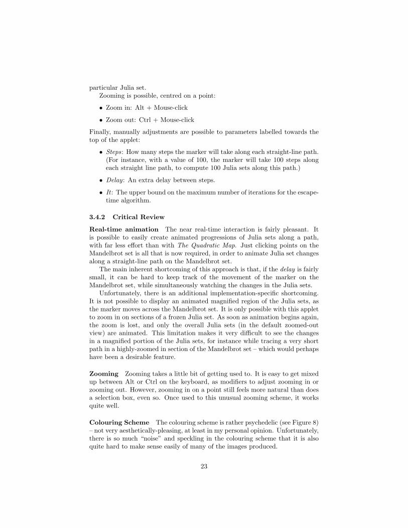
Figure 9: Screenshot of Mandelbrot Maps

4.1 Initial Design

Mandelbrot Maps – the applet created for this MSc project – was intended fromthe beginning to avoid some of the pitfalls encountered by previously-existingapplets, while adding in some useful features too. The overall aim was to create

24



an applet which was very easy to use, and which allowed useful, easy explorationof the Mandelbrot set and associated Julia sets.

In initially planning the applet, my belief from the beginning was that real-time interaction would be desirable – most especially in the generation of theJulia sets. (This hypothesis, of real-time interaction being preferred by endusers, is examined with a user evaluation, detailed in section 5.)

The important questions at the initial planning stage therefore included:Can real-time interaction be achieved? What image quality can we hope for?What broad architecture should we use?

4.1.1 Overall Architecture

It was unclear at this stage whether it would be necessary to exploit multiplecomputers working in parallel, for instance, if there was to be any hope ofgenerating timely real-time images. It was also unclear whether Java would bea suitable language to use4.

4.1.2 Creating a Prototype

For this reason, a simple-minded prototype Java applet was written at the earli-est design stage, before continuing any further. Figure 10 is a screenshot of thisprototype. (This prototype turned out to be the basis of Mandelbrot Maps –which developed through a long series of improvements, of varying complexity,to this initial code.)

The Mandelbrot set is displayed on the left. Mousing over a point in theMandelbrot set led to a new Julia set being displayed on screen, correspondingto the point being moused over.

The images displayed are greyscale, with the intensity of each pixel propor-tional to the percentage of the maximum number of iterations that would becarried out required to see the relevant orbit first go outwith a circle of radius 2– ie, diverge. This is the escape-time algorithm, described in 2.1.2, with almostthe simplest-possible colouring algorithm.

This prototype could be run in any arbitrary size. Larger sizes meant thatmore computations had to be performed, to display each Julia set image, sincemore pixels had to be computed. The number of pixels increases as the squareof the width of a square-shaped viewing area, so doubling the viewing area leadsto four times the number of pixels to compute and display. This correspondsto considerably more computational work, if we make the (reasonable) assump-tions that the average amount of work per pixel doesn’t substantially change onvarying viewing area resolution, and that the chief bottleneck is the time taken

4Java has something of a reputation for being slow. After having used Java for thiscomputationally-intensive project, I now believe this reputation is undeserved – an urbanmyth, perhaps arising due to Java’s earliest versions’ poor performance, and the sometimes-slow startup time of the Java Virtual Machine. There are some interesting benchmarks in[8], and I agree with most of the arguments made; it makes interesting reading, albeit onlytangentially-relevant to this project.

25

Figure 10: Mandelbrot Maps – screenshot of earliest prototype.

to perform all of the behind-the-scenes iterations (rather than, say, the screenupdate frequency).

4.1.3 Lessons from the Prototype

Using this prototype, it was discovered that:

• An upper bound of approximately 100 iterations is sufficient to display agood Julia set image, at this “big picture” zoomed-out scale.

• A single modern desktop computer (CPU: E6750 Intel Core 2 Duo CPU @2.66Ghz) is quite capable of generating timely Julia set images of reason-able resolution (at 400× 400 pixels, 3 images/second) on this zoomed-outscale, inside a Java applet.

Another discovery – arguably just as important – was that this two-panelledapproach with real-time display, based on mouse movements across the Man-delbrot set, indeed felt very natural, especially when compared to the already-experienced pre-existing non-real-time applets.

Heartened by the success of this first prototype, the Informatics ReviewReview was written at this stage in the development of Mandelbrot Maps, anddevelopment could then continue in earnest.

4.2 Zooming

A crucial feature addition was zooming : both on the Mandelbrot set, and on agenerated Julia set image.

Note that to fully implement zooming, there are some complications. Forinstance, to generate accurate pictures at high zoom levels on non-trivial areas

26

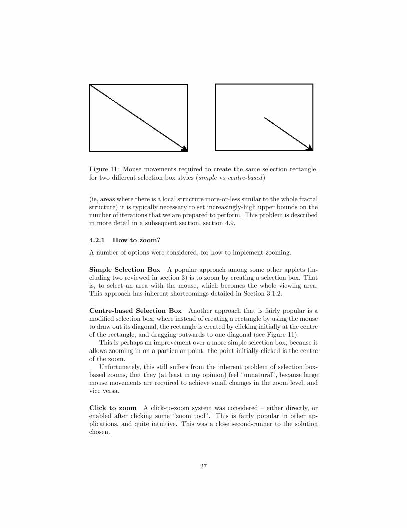
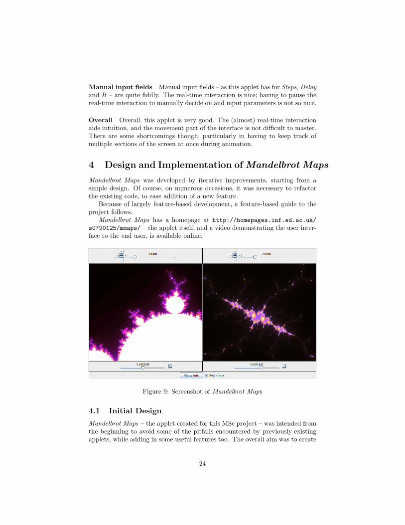
Figure 11: Mouse movements required to create the same selection rectangle,for two different selection box styles (simple vs centre-based)

(ie, areas where there is a local structure more-or-less similar to the whole fractalstructure) it is typically necessary to set increasingly-high upper bounds on thenumber of iterations that we are prepared to perform. This problem is describedin more detail in a subsequent section, section 4.9.

4.2.1 How to zoom?

A number of options were considered, for how to implement zooming.

Simple Selection Box A popular approach among some other applets (in-cluding two reviewed in section 3) is to zoom by creating a selection box. Thatis, to select an area with the mouse, which becomes the whole viewing area.This approach has inherent shortcomings detailed in Section 3.1.2.

Centre-based Selection Box Another approach that is fairly popular is amodified selection box, where instead of creating a rectangle by using the mouseto draw out its diagonal, the rectangle is created by clicking initially at the centreof the rectangle, and dragging outwards to one diagonal (see Figure 11).

This is perhaps an improvement over a more simple selection box, because itallows zooming in on a particular point: the point initially clicked is the centreof the zoom.

Unfortunately, this still suffers from the inherent problem of selection box-based zooms, that they (at least in my opinion) feel “unnatural”, because largemouse movements are required to achieve small changes in the zoom level, andvice versa.

Click to zoom A click-to-zoom system was considered – either directly, orenabled after clicking some “zoom tool”. This is fairly popular in other ap-plications, and quite intuitive. This was a close second-runner to the solutionchosen.

27

Mouse wheel to zoom An approach gaining popularity among other appli-cations is using the mouse wheel to zoom. Because a mouse wheel moves intwo directions, one direction can indicate a zoom in, and the other direction azoom out. A person can then mouse over a particular point and use the mousewheel to zoom in/out, centred on this point. In my personal opinion, this is anextremely natural way of zooming.

Notably, this approach is used in Google Maps[2] (which is where my ex-posure to this mouse-wheel idea came from), and it also seems to be gainingpopularity elsewhere. For instance, it is also used in the open-source Eye ofGNOME [1], the default GNOME image viewer.

4.2.2 Implementing Mouse Wheel Zooming

Having decided to use mouse wheel based zooming, there was no great difficultyin implementation. A constant zoom-factor approach was used, where eachzoom step magnified the area (centred on the point being moused over) by aconstant percentage.

This algorithm was straightforward to implement: decrease in turn the dis-tance of each of the four edges of the current viewing area from the zoom centre(the point being moused over) by a constant percentage5, then set this area asthe new viewing area and redraw.

4.2.3 Zoom Limits

There are limitations of arithmetic using Java’s doubles: Mandelbrot Maps doesnot perform arbitrary-precision arithmetic, but rather limited-precision arith-metic, using Java’s native double type. Therefore, beyond a certain zoom scale,errors accumulate to such an extent that they dominate the attempt at imagegeneration.

These errors manifest themselves as blocky lines, where some adjacent pixelsincorrectly take on the same colours (as determined by the escape-time algo-rithm). This imposes a limit on how far it is meaningful to attempt to zoom in,no matter what upper bound is set on the number of iterations to perform.

This limit is empirically observed to limit zooming to approximately a tril-lion times (12 orders of magnitude) for the Mandelbrot set, and 100 milliontimes (8 orders of magnitude) for the Julia set – the difference in the orders ofmagnitude being due to the difference in the rate at which errors accumulatefor the calculations of the orbits of the relevant points, in each case, with thedifferent iterated equation.

Mandelbrot Maps has these limits coded in, and will refuse to zoom in anyfurther once they are reached. Similarly, a maximum sensible limit for zoomingout is also imposed – so that the user does not accidentally zoom out far furtherthan would make any sense (say, to a region in which the whole fractal occupiesonly a pixel of the display).

5A zoom out is a straightforward generalisation – where the percentage decrease in dis-tances is negative, causing an overall increase in the viewing area.

28

4.3 Zoom Slider

Because zooming is implemented, and because limits have been imposed forhow far we may zoom in or zoom out, a logarithmically-scaled zoom slider is asensible addition to the top of each panel: one for the Mandelbrot set; one forthe Julia sets.

The main function of the zoom slider is orientation, in two different ways:

• The slider offers a quick “at a glance” indication of how zoomed-in we are.

• It is possible to manipulate the slider directly, to zoom in or zoom out –this time, centred on the canvas centre. Because the zoom centre is theexact canvas centre, it is possible to slide the zoom slider to zoom out asfar as we wish, and then slide it the other way to zoom straight back in tothe original point we started from6. This is a very handy feature, as wecan see quickly view a zoom in to a point we found, from any arbitrarilyzoomed out scale that we wish.

4.4 Panning (moving around the canvas)

To pan the canvas – move the canvas – the approach used by Google Maps[2](among others) is again used. Specifically, click-and-drag is used to move thecanvas. The point under the mouse is kept constant, and the rest of the canvasis moved appropriately.

This neatly ties in with the zoom wheel being used to scroll. It is, in bothcases, possible to manipulate the canvas directly, and in a very natural manner.

In addition, navigation buttons (up, down, left, right) were placed near tothe zoom slider, and can alternatively be used for movement.

4.5 Home Button

Next to the navigation buttons, a home button was added. When clicked, thedefault view is restored: a zoomed-out display of the whole fractal image.

4.6 Save

A useful feature, and one which seems to be often omitted in other applets, isthe ability to save the images that it displays.

6This is also possible when zooming with the mouse wheel, if care is taken not to movethe mouse at all while manipulating the scroll wheel. It is challenging to keep the mouseexactly still though, and movements – even by a pixel – will change the zoom centre, whichwill certainly be problematic if this movement occurs when zoomed out quite a way: we willhave lost the original point that we wanted to zoom back in on, when we changed the zoomcentre by moving the mouse.

29

4.6.1 Variety of Resolutions

Mandlebrot Maps is capable of generating images for saving at a variety ofresolutions, which are labelled as:

• Small (approximately 475×406 pixels – this is always set to the exact sizeof the canvas, as seen on screen)

• Medium (1024× 768 pixels)

• Large (1600× 1200 pixels)

• Large - Widescreen (1680× 1050 pixels)

• Extra Large (1920× 1200 pixels)

• Extra Large - Widescreen (2560× 1600 pixels)

The rationale for allowing multiple sizes is that a person may wish to generatea high-resolution image, for display in some way – for instance, as a desktopbackground, as an image on a poster, or as part of a full-screen slideshow.

Image Area When the aspect ratio of the canvas does not match that of theimage to be saved, what area should the image show? (Note that this discussesthe image’s viewing area, not any actual transformations carried out on somein-memory image. The images are then generated on the fly, by performing thestandard iteration-count algorithm, after having set the viewing area.)

Care must be taken to neither clip the on-screen viewing area – which mayresult in the loss of a feature we were interested in – nor to stretch the canvas– which would result in distorted shapes.

The approach adopted by Mandelbrot Maps is illustrated in Figure 12. Thefractal image on screen is represented by a red box, with a blue circle in it. Thelarge rectangle represents the image area.

30

Figure 12: Centre the scaled-up canvas within the full image area. This is theapproach used in Mandelbrot Maps. There is no truncation of the on-screenimage, nor is there stretching resulting in distorted shapes.

Image-saving considerations There are two more considerations for savingimages:

• Generating a high-resolution may take a long time. Therefore, MandelbrotMaps carries out the computations in a low-priority thread, behind thescenes – with a progress bar to show how much of the image has beengenerated. The progress bar also has a Cancel option, allowing the userto abort the rendering.

• Applets are limited for memory by the Java Virtual Machine. A typicallimit (default on installation, though it can be adjusted) is about 64MB.Because the images are generated in-memory as large bitmaps, the appletmay run out of memory when trying to allocate space to generate a newimage. To try to reduce the chances of this happening unnecessarily, Javais asked to garbage-collect just before the memory for a new bitmap isallocated. If we run out of memory even so on attempting the allocation,an error message is displayed, advising the user to save the image at asmaller size or to wait for other image(s) being generated to completefirst.

4.7 Bookmarking: Show URL

Another oft-overlooked feature in fractal explorers is the ability to return to anice location that you have found. That is, the ability to in some way bookmarkthe current location, and possibly even send it to a friend.

31

Three options were considered for Mandelbrot Maps:

• Save/load text files, containing the internal location data in some form.This would work, but perhaps it is non-ideal to use a custom text-fileformat.

• Save/load self-documenting XML files, containing the internal locationdata as before. This would work, but exchanging files with a friend isperhaps not ideal – especially because it would require the friend to knowwhere to find the applet already, and then to open the XML file in theapplet.

• Generate self-documenting URLs, which consist of the applet’s URL alongwith parameters representing location data passed in the query string.This is the approach used by Mandelbrot Maps.

To generate a URL, there is a Show link button. When clicked, a URL isdisplayed in a textbox, ready to be copy-and-pasted elsewhere – for instance, inan instant message or an email to a friend.

The URL contains all the state information about the current location, andso is able to restore this state when loaded.

4.8 Colouring the Image

As discussed in Section 2.1.2, the escape time algorithm generates as its outputfor each pixel an iteration percentage: the percentage of the maximum iterationsthat were computed for this particular point, before a point that strayed outsidethe circle of radius 2 was first found. Pixels with percentages of <100% areguaranteed to be outside the set; the lower the percentage, the greater thepoint’s “distance” from the set. Pixels with percentages of 100% are assumedto be within the set (or at least rather close to the set – so close that we cannottell that they are not within the set, without re-running the algorithm with ahigher upper bound of iterations).

The goal now is to colour these pixels in such a way, starting from theseinput percentages, to produce an image that hopefully:

• Aids intuition

• Is aesthetically-pleasing

In creating Mandelbrot Maps, various colouring methods were tried.

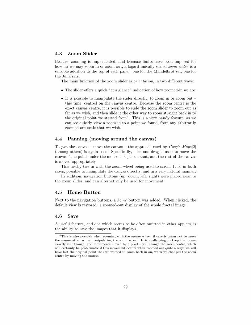
Greyscale The simplest way to colour the image is to set the pixel’s inten-sity proportional to the iteration percentage (100% corresponding to white; 0%corresponding to black; greys in between). The result is a greyscale image, suchas Figure 13.

This works, but could be improved with the addition of colour.

32

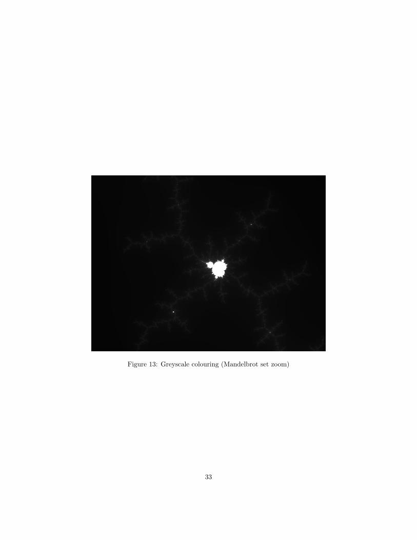
Figure 13: Greyscale colouring (Mandelbrot set zoom)

33

Figure 14: HSV colour space: hue varying with the number of iterations (Man-delbrot set zoom)

HSV Colour Space The next attempt was to use the hue-saturation-value(HSV) colour space. The saturation and value were fixed, while the hue wasdetermined straighforwardly from the iteration percentage7. This led to resultssuch as in Figure 14.

While certainly colourful, this is not in my opinion very aesthetically-pleasing.The result is garish, to my eyes.

RGB Colour Space I moved to the red-green-blue (RGB) colour space,where pixel colours are determined based on independently-set intensities forred (R), green (G) and blue (B) colour components; each component’s intensitybeing represented by an integer in range 0 – 255. The question thus became:what mathematical functions would be good to use to map an iteration per-centage to an integer in range 0 – 255, for each of the R, G and B colourcomponents?

The most straightforward answer, of using for each component a simplescaling up from the iteration percentage to the range 0 – 255, is a way of againgenerating simple greyscale images such as Figure 13.

7The hues in this colour space may be laid out in a finite line. The percentage of iterationsperformed thus trivially maps to a unique point on this line: to a hue.

34

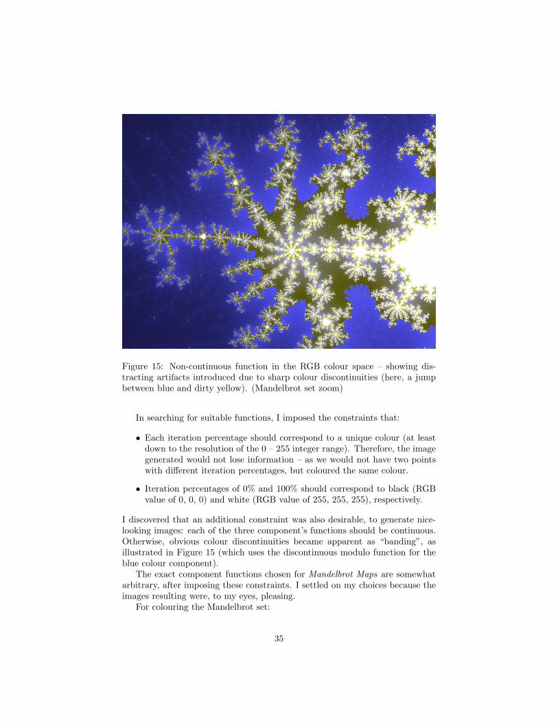
Figure 15: Non-continuous function in the RGB colour space – showing dis-tracting artifacts introduced due to sharp colour discontinuities (here, a jumpbetween blue and dirty yellow). (Mandelbrot set zoom)

In searching for suitable functions, I imposed the constraints that:

• Each iteration percentage should correspond to a unique colour (at leastdown to the resolution of the 0 – 255 integer range). Therefore, the imagegenerated would not lose information – as we would not have two pointswith different iteration percentages, but coloured the same colour.

• Iteration percentages of 0% and 100% should correspond to black (RGBvalue of 0, 0, 0) and white (RGB value of 255, 255, 255), respectively.

I discovered that an additional constraint was also desirable, to generate nice-looking images: each of the three component’s functions should be continuous.Otherwise, obvious colour discontinuities became apparent as “banding”, asillustrated in Figure 15 (which uses the discontinuous modulo function for theblue colour component).

The exact component functions chosen for Mandelbrot Maps are somewhatarbitrary, after imposing these constraints. I settled on my choices because theimages resulting were, to my eyes, pleasing.

For colouring the Mandelbrot set:

35

Figure 16: RGB component functions used in Mandelbrot Maps – Mandelbrotset

Green Simple scaling, from iteration percentage to range 0 – 255.

Red Steep scaling, from iteration percentage to range 0 – 255, hitting the ceilingvalue of 255 before an iteration percentage of 100% (20%), and remainingat the maximum value of 255 thereafter.

Blue Sinusoidal function, shifted and scaled such that 0% corresponds to 0,and 100% corresponds to the ceiling value of 255.

This is graphically represented in Figure 16. Note that all three constraints aremet (distinct colours for a given iteration percentage, black/white endpoints,continuous component functions). This is the approach used to colour the Man-delbrot images, with results such as Figure 17.

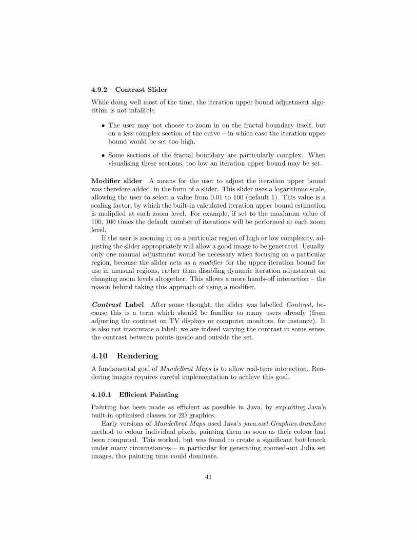
A very similar, but distinct, choice of component functions is used for colour-ing the Julia sets. The rationale here is that using a slightly different colourscheme provides a visual cue to users that the Mandelbrot set and the Julia setsare not the same (albeit related).

The Julia sets’ colour scheme is represented graphically in Figure 18, and anexample generated image is shown in Figure 19.

4.9 Number of Iterations to Perform

The escape time algorithm (see Section 2.1.2) needs an upper bound on thenumber of iterations that will be performed. What should this limit be?

If the limit is set too low, we generate misleading images – with lots of pointsclose to the Mandelbrot set being miscategorised as within the Mandelbrot set.If set too high, we may perform considerable unnecessary work – iterating pointsmore times than are necessary to obtain a good image.

36

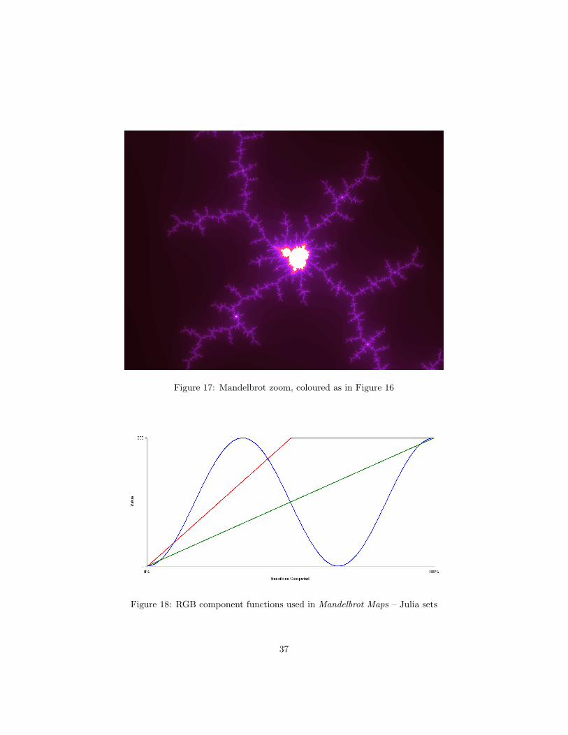
Figure 17: Mandelbrot zoom, coloured as in Figure 16

Figure 18: RGB component functions used in Mandelbrot Maps – Julia sets

37

Figure 19: Julia zoom, coloured as in Figure 18

38

One approach is simply to allow the user to input directly the upper boundon number of iterations. This is an approach taken by many other fractalexplorers. However, can we do better? Can we determine how many iterationswe will likely need to perform, without user input?

Two observations which I made suggest that we can automate selecting anappropriate number of iterations, at least to some extent.

1. The “interesting” images are found when zooming in on the fractal bound-ary, rather than on either “empty space” or the featureless set interior.Therefore, a reasonable assumption is that people will tend to be zoomingin on or very near to the fractal boundary, at least most of the time.

2. The further we are zoomed in on the fractal boundary, the higher theiteration limit needs to be set in order to produce accurate shapes. Intu-itively, this makes some sense – the further we are zoomed in on the fractalboundary, the “closer” the points are to the interior of the set, and so themore iterations we will need to carry out to be able to classify points asinside or outside the set.

4.9.1 Quantifying the Iteration Upper Bound

By eye, I noted how many iterations were necessary to create a “good” imagefor the Mandelbrot set or various Julia sets, at various levels of zoom on thefractal boundary.

The results are shown graphically in Figures 20 and 21, for the Mandelbrotand Julia sets respectively. Note that the scales are logarithmic: the plots showthe logarithm of the needed iteration upper bound (judged by eye) versus themagnitude of the logarithm of the width of each pixel, while zooming in on thefractal boundaries.

We have quite a good straight-line fit on each log-log plot:

Mandelbrot set Based on the trendline in Figure 20:

ln(iterations) = 0.2095 |ln(pixelSize)|+ 3.998

∴ iterations = 54e1.23|ln(pixelSize)|

Julia set Based on the trendline in Figure 21:

ln(iterations) = 0.4588 |ln(pixelSize)|+ 1.8662

∴ iterations = 6.46e1.58|ln(pixelSize)|

These trend-lines are therefore coded into Mandelbrot Maps, and used todynamically set the iteration count upper bound, at each zoom level.

39

Figure 20: Plot showing iterations upper limit needed to obtain a “good” visu-alisation of the Mandelbrot set fractal boundary, at various scales.

Figure 21: Plot showing iterations upper limit needed to obtain a “good” visu-alisation of Julia set fractal boundaries, at various scales.

40

4.9.2 Contrast Slider

While doing well most of the time, the iteration upper bound adjustment algo-rithm is not infallible.

• The user may not choose to zoom in on the fractal boundary itself, buton a less complex section of the curve – in which case the iteration upperbound would be set too high.

• Some sections of the fractal boundary are particularly complex. Whenvisualising these sections, too low an iteration upper bound may be set.

Modifier slider A means for the user to adjust the iteration upper boundwas therefore added, in the form of a slider. This slider uses a logarithmic scale,allowing the user to select a value from 0.01 to 100 (default 1). This value is ascaling factor, by which the built-in calculated iteration upper bound estimationis muliplied at each zoom level. For example, if set to the maximum value of100, 100 times the default number of iterations will be performed at each zoomlevel.

If the user is zooming in on a particular region of high or low complexity, ad-justing the slider appropriately will allow a good image to be generated. Usually,only one manual adjustment would be necessary when focusing on a particularregion, because the slider acts as a modifier for the upper iteration bound foruse in unusual regions, rather than disabling dynamic iteration adjustment onchanging zoom levels altogether. This allows a more hands-off interaction – thereason behind taking this approach of using a modifier.

Contrast Label After some thought, the slider was labelled Contrast, be-cause this is a term which should be familiar to many users already (fromadjusting the contrast on TV displays or computer monitors, for instance). Itis also not inaccurate a label: we are indeed varying the contrast in some sense;the contrast between points inside and outside the set.

4.10 Rendering

A fundamental goal of Mandelbrot Maps is to allow real-time interaction. Ren-dering images requires careful implementation to achieve this goal.

4.10.1 Efficient Painting

Painting has been made as efficient as possible in Java, by exploiting Java’sbuilt-in optimised classes for 2D graphics.

Early versions of Mandelbrot Maps used Java’s java.awt.Graphics.drawLinemethod to colour individual pixels, painting them as soon as their colour hadbeen computed. This worked, but was found to create a significant bottleneckunder many circumstances – in particular for generating zoomed-out Julia setimages, this painting time could dominate.

41

Refactoring to use java.awt.image.MemoryImageSource improved performancegreatly, in these cases (benchmarked at 20 images/second vs 3 images/secondfor a typical zoomed-out Julia set image, all other factors being equal, on a com-puter with E6750 Intel Core 2 Duo CPU @ 2.66Ghz). MemoryImageSource isa Java class optimised for good graphics performance, when used for animatedgraphics based on in-memory pixel grids.

4.10.2 “Blocky Squares” Crude-first Rendering

Exponentially-increasing work As discussed in Section 4.9.1, typical zoom-ing in on the fractal boundary results in an exponentially-increasing upperbound to the maximum number of iterations in the escape-time algorithm. Gen-erating a full image in anything approaching real-time (say, under 0.5 seconds)therefore rapidly becomes impossible.

To mitigate this problem, we may first generate a cruder “blocky” rendering,before later carrying on to fill in the details with a full-quality rendering.

Pixel blocks If, instead of computing a colour for every pixel, we instead firstcomputed the same image area but made up out of 2 × 2 pixel blocks, we willbe performing around about 1

2×2 = 14 the calculations. Therefore, we would

expect the cruder 2 × 2 block rendering to be ready about 4 times faster thanthe full-quality rendering.

Similarly, we would expect a 3×3 block rendering to be about 9 times fasterthan the full-quality rendering; a 4 × 4 block rendering to be about 16 timesfaster; etc.

To allow real-time interaction at greater zoom levels than would otherwisebe possible, Mandelbrot Maps therefore carries out a cruder “blocky” renderingfirst, before filling in the details later. The block size is increased as the max-imum number of iterations that might be carried out increases. Furthermore,the high-quality rendering may be interrupted before it completes.

On a fairly modern computer (with E6750 Intel Core 2 Duo CPU @ 2.66Ghz)this allows real-time interaction over the wide range of zoom levels supported inMandelbrot Maps – with the limits being imposed by the precision of the doubletype, as described in Section 4.2.3.

4.10.3 Rendering Threads

Mandelbrot Maps performs the time-consuming iteration calculations in a sep-arate thread, so as to allow the GUI to remain responsive at all times. If thesecalculations were performed in the main thread, then the GUI would becomeunresponsive while rendering was in progress.

Rendering Queue A thread-safe blocking FIFO (first-in, first-out) queue ofscheduled renderings is used, one queue for each panel: one queue for the Man-delbrot set panel; one queue for the Julia set panel. Each panel also has an

42

associated rendering thread, which sequentially processes its queue, one render-ing at a time.

The unprocessed scheduled renderings in the queue may be cleared beforescheduling a new rendering, for the reason that these renderings are now out ofdate, and should not be started. (For instance, if the mouse is rapidly movedover the Mandelbrot set, a string of Julia sets will have rendering scheduled.We should not begin rendering an out-of-date Julia set corresponding to an oldmouse position, when we have a newer Julia set to render; we should emptythese old, unstarted renderings out of the queue.)

The rendering thread may be pre-emptively aborted at any time while per-forming the high-quality rendering. Therefore, if a new rendering is scheduledwhile a high-quality rendering is in progress, the old high-quality rendering maybe aborted so that the new rendering may begin at once.

While performing a crude rendering, though, the rendering thread will notabort until at least 300ms has passed, even if a new rendering has appeared.In earlier versions of Mandelbrot Maps, the crude rendering was either neverpre-emptively aborted (which caused unresponsiveness if the crude renderingdid, for any reason, take a significant amount of time), or was always able to bepre-emptively aborted (which caused problems because it was easy to create asituation where no renderings were completed, since each rendering would needjust a few milliseconds more time than available to complete).

Why 300ms? 300ms is a compromise value picked for human reasons, andone which suited my personal taste. It would be possible to perform a userevaluation to perhaps tweak and improve on this value, but this would requiremore resources and time than available in this project.

A somewhat reasonable choice of this value would, I believe, be in the ball-park range of 100ms – 1000ms. To put that more quantitatively: I think itcould be 200ms or 500ms, but not 100ms or 800ms - making the assumptionthat my personal preferences are not very far away from “human norms”.

With a low value like 100ms, crude renderings would be considerably lesslikely to complete successfully due to the more strict cut-off – especially on aslower CPU. With a high value like 1000ms, crude renderings would be slightlymore likely to complete successfully, but the delay may become very cumber-some. 300ms was the best compromise that I found after some brief trial-and-error, for my personal taste.

This delay is most seen when using the zoom slider to zoom out/in on apoint for orientation. The crude renderings shown here need to be timely, butneed a fair chance to complete too. If not given a chance to complete, thatis if crude renderings may always be aborted (a value of 0ms!), when movingthe zoom slider, there may be no real-time feedback at all, as a chain of cruderenderings are all pre-empted without any completing.

Allowing interruption is perhaps most useful as a safety mechanism to catchthe rare condition of a very slow crude rendering. When zoomed in a long way,and turning the contrast up very high, the associated crude rendering may take

43

longer than 300ms to complete. Allowing pre-emptive abortion if the contrastslider is decreased (when the user realises that “this isn’t a good idea” and triesto lower the contrast slider to a more sensible place) allows Mandelbrot Mapsto remain responsive to this change, by aborting the slow crude rendering.

High-quality rendering feedback If a high-quality rendering takes a sig-nificant amount of time – which is here chosen to mean over 300ms for similarreasons to before – then the work in progress is shown at regularly. That is,a “sweeping down” is seen, as the high quality rendering is generated (whichis not guaranteed to complete, since it may be pre-emptively aborted at anytime if the user requests a different rendering). This acts as visible feedback toshow that something is happening, and to let the user immediately see whathigh-quality rendering data the computer has already computed as soon as it isavailable.

5 User Evaluation

To gain feedback from real users about Mandelbrot Maps, and in the process togain data to test the hypothesis that real-time interaction is indeed generallypreferred by users, a user evaluation was performed.

5.1 Method

A real-time tickbox was added to the Mandelbrot Maps interface – it is visiblein Figure 9, near the bottom of the applet.

5.1.1 Real-time Tickbox Features

By default, this box is ticked – so that Mandelbrot Maps runs in real-time mode.In this mode, real-time features are enabled:

• An initial crude fast blocky rendering (section 4.10.2) is used, if necessary.A full-quality rendering then completes afterwards.

• Julia sets are displayed in real time, on moving the mouse within theMandelbrot set.

• Panning around the canvas is possible with click-and-dragging (section4.4), and zooming with the mouse wheel (section 4.2). (Note that naviga-tion buttons still do appear, to be used if preferred.)

• The zoom slider (section 4.3) and the contrast slider (section 4.9.2) updatethe display in real-time when modified.

When this box is not ticked – so that Mandelbrot Maps is running in non-real-time mode, the real-time specific features are disabled. Now:

44

• No fast, crude rendering is displayed; just the high-quality, slow rendering.

• Julia sets are displayed when clicking the mouse within the Mandelbrotset.

• Moving around the canvas is possible only with the navigation buttons,and zooming only with the zoom slider.

• The zoom slider and contrast slider do not provide real-time feedback;the display updates only once a value has been chosen, rather than whilemodifying the slider value.

The home (section 4.5), save (section 4.6) and show link (section 4.7) featuresare the same in both modes.

5.1.2 Why the two modes?

This tickbox allows toggling on or off the real-time features of Mandelbrot Maps,while keeping the rest of the interface the same. As fair a test as possible couldthen be performed, between a real-time and a non-real-time applet – as it is allthe same applet, just running in different modes.

Otherwise, if a comparison had been made between Mandelbrot Maps anda second non-real-time applet, all sorts of confounding factors could enter in– such as a user voting up one applet over the other because of preferring itscolour scheme. In this way, all other factors could be kept constant, to judgeuser feedback on the real-time features alone.

5.1.3 Survey

A link to http://homepages.inf.ed.ac.uk/s0790125/mmaps/ (the home ofMandelbrot Maps) was advertised. From here, a self-selected group of interestedvolunteers could:

• View a brief quick-start guide to using the features of the MandelbrotMaps interface, in a 4 minute screencast which I created and uploaded toYouTube: http://www.youtube.com/watch?v=pMCB4C_dVyI

• Experiment with Mandelbrot Maps itself – which the screencast encour-aged them to do in both real-time and non-real-time modes: http://homepages.inf.ed.ac.uk/s0790125/mmaps/mmaps.html

• Fill in a brief survey about their experiences: http://homepages.inf.ed.ac.uk/cgi/s0790125/mmaps.html

The survey asked users:

• How many minutes they had spent using Mandelbrot Maps

• To rate the image quality (0 – 10 scale)

45


http://www.youtube.com/watch?v=pMCB4C_dVyI

http://homepages.inf.ed.ac.uk/s0790125/mmaps/mmaps.html

http://homepages.inf.ed.ac.uk/s0790125/mmaps/mmaps.html

http://homepages.inf.ed.ac.uk/cgi/s0790125/mmaps.html

http://homepages.inf.ed.ac.uk/cgi/s0790125/mmaps.html

• To rate real-time and non-real-time modes for their ease of use (0 – 10scale)

• To rate real-time and non-real-time modes overall (0 – 10 scale)

• To select which of the following features they understood how to use:

– Moving (left, right, up, down)

– Zoom

– Save

– Generating a link

– Adjusting the contrast

• Whether the person had ever used other programs to explore fractals

• To rate their own computer abilities

• For any other comments

• For their email address – optionally, so that it could be filled in anony-mously if preferred

Explaining the mathematics behind the Mandelbrot set, and the Julia sets, wasout of scope for the user survey, however. There are numerous other webpagesavailable which detail this, and users filling in the survey were not required tohave familiarity with the mathematics. The hope was that, in spite of this, theuser interface would be sufficiently clear to allow intuitive exploration of thefractals, even if the user was unfamiliar with the maths behind the images.

5.1.4 Advertising the survey

A wide range of people were invited to take part in the survey. This included:

• All Informatics students – both undergraduate and postgraduate – at theUniversity of Edinburgh, as of July 2008

• Friends and family (with a wide range of computer or mathematical ex-perience)

• Linking internet communities with perhaps interested audiences (http://forums.outpost10f.com/ and http://forums.xkcd.com/)

In all, 89 survey responses were received – from a wide variety of users, fromthese various backgrounds.

46

http://forums.outpost10f.com/

http://forums.outpost10f.com/

http://forums.xkcd.com/

Figure 22: How survey respondents rated their computer abilities

5.2 User Feedback

The vast majority of users were able to run the applet with no difficulty. This isgood – as it was a key motivation behind the decision to implement MandelbrotMaps as a Java applet.

Unfortunately, there was a problem for some Mac users: some older Macs,used by early adopters, cannot yet run Sun’s Java 1.6, and therefore were unableto run Mandelbrot Maps. This problem was reported to me by three Mac users.

5.2.1 User Base

Based on the survey responses:29% of the respondents had used fractal explorers before.89% of respondents answered the question How many minutes have you spent

using this program, Mandelbrot Maps? : their mean time spent using MandelbrotMaps before filling in the survey was 9 minutes. (This is perhaps what wouldbe expected for casual and interested, but busy, volunteers.)

Nearly all respondents rated their personal computer abilities as somewherebetween average (5/10) and expert (10/10): see Figure 22. Note, however, thatthe question How would you rate your own computer abilities? is very sub-jective, and this question’s answers should perhaps not be taken too seriously.This graph (Figure 22) is shown only to illustrate that most people answeringthe survey regarded themselves as average or above, but with a large spread ofresponses to this question.

5.2.2 Features Understood

Respondents answered the survey question Please select the features of Mandel-brot Maps that you understand how to use. Percentages of respondents claiming

47

to understand how to use the various features follow:

• Move – 99%

• Zoom – 97%

• Save Image – 82%

• Show Link – 73%

• Adjust Contrast – 91%

It is very encouraging to note that the overwhelming majority of respondentsunderstood how to use the basic interface: to move and zoom.

The contrast slider also was widely understood. (It was not mentioned inthe introductory video that the slider adjusted the upper bound on the numberof iterations to perform, but people could seem to intuitively understand thatadjusting the slider could present extra detail, when necessary.)

Saving images and showing links presented a little more trouble to somepeople, but were still understood by most respondents.

5.2.3 Comments

The response was overwhelmingly positive. A lot of very positive commentswere received. Samples from many of these comments are quoted below.

From people with prior experience with fractal applets:

• I find the Mandelbrot set one of the most accessible illustrations of thebeauty of mathematics, and I have tried to get people interested in thesubject using various Mandelbrot set explorers on the net. This is in adifferent league. I am extremely impressed.

• The rating system should allow for higher than 10 scores.

• This program was phenomenal. Brilliant brilliant job.

• Very cool. Particularly as you have it running as a java applet, it’s reallynice and smooth (surpringly!). Good clear GUI and the real time versionis very natural to use.

• Very good and easy to use....!

• Very impressive!

From people without any prior experience with fractal applets:

• I love the colours!

• Way kewl program!!! Now I have a new background on my desktop!!

48

• I said I’ve used other fractal programs. I have: Apophysis (for use byfractal artists). It made no real sense to me and I haven’t managed toactually use it, but I understand the whole fractal concept better nowafter this. So whether that was intentional or not, thanks!

• twas fun!

• This is incredibly cool! I’ve never seen anything like this before, but Ithink it’s fun to play with.

• The applet is amazing!

• i find the quality of the images very clear and very detailed and the rangeof the zoom to within billions of the image is very impressive good luckwith it

• Quite beautiful. You should work with an artist to fully explore thispotential. I still don’t understand what a Mandelbrot set is. How is thisconnected to daily life? Regardless, Well done, you made this very userfriendly.

• Nice App, might have to go and look up what mandelbrot sets and juliasets are now you’ve sparked my interest.

• Very fun and pretty (I now have a Mandelbrot desktop wallpaper), I cansee it being quite addictive looking at how each point varies. It would beinteresting if it was extended with other fractals and a little informationabout the different types.

• Great fun - thanks. Will pass it on.

• A very good piece of work - Kudos!

• One of the cooler things I’ve seen in quite some time. Fractals are moreinteresting than I originally thought.

In particular, it is worth noting that a few respondents found the images suf-ficiently aesthetically pleasing that they were worthy images for being used astheir new desktop background! It is hard to find higher praise than this.

5.2.4 Image Quality

More quantitatively than noting that some respondents were so pleased with theimages that they deemed them worthy of being used as desktop backgrounds,the results of the respondents being asked to rate the image quality on a scale of0 (very poor) – 10 (excellent) are available. These results are shown graphicallyin Figure 23.

The two users who rated the image quality as 0 had submitted the surveywithout being able to run the applet at the time of responding, due to nothaving Java 1.6 correctly installed.

49

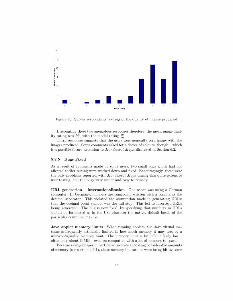
Figure 23: Survey respondents’ ratings of the quality of images produced

Discounting these two anomalous responses therefore, the mean image qual-ity rating was 8.0

10 , with the modal rating 1010 .

These responses suggests that the users were generally very happy with theimages produced. Some comments asked for a choice of colours, though – whichis a possible future extension to Mandelbrot Maps, discussed in Section 6.2.

5.2.5 Bugs Fixed

As a result of comments made by some users, two small bugs which had notaffected earlier testing were tracked down and fixed. Encouragingly, these werethe only problems reported with Mandelbrot Maps during this quite-extensiveuser testing, and the bugs were minor and easy to remedy.

URL generation – internationalisation One tester was using a Germancomputer. In Germany, numbers are commonly written with a comma as thedecimal separator. This violated the assumption made in generating URLs:that the decimal point symbol was the full stop. This led to incorrect URLsbeing generated. The bug is now fixed, by specifying that numbers in URLsshould be formatted as in the US, whatever the native, default locale of theparticular computer may be.

Java applet memory limits When running applets, the Java virtual ma-chine is frequently artificially limited in how much memory it may use, by auser-configurable memory limit. The memory limit is by default fairly low –often only about 64MB – even on computers with a lot of memory to spare.

Because saving images in particular involves allocating considerable amountsof memory (see section 4.6.1), these memory limitations were being hit by some

50

users, but the java.lang.OutOfMemoryError was not handled in any way; imagesaving just failed silently.

Now, java.lang.OutOfMemoryError is caught, and an appropriate error mes-sage is displayed (advising the user to save only one or two images at a time, orto save the image in a smaller size). Also, Java’s built-in garbage collection isinvoked before allocating memory for new images to save, in the hope that asmuch memory as possible will be freed, to maximise the chance of the memoryallocation succeeding.

5.3 Testing the Real-time Hypothesis

I hypothesised that people would prefer real-time interaction, to non-real-timeinteraction. More specifically, I hypothesise that users overall will rate real-timemode higher than non-real-time mode for both ease of use and overall. The nullhypothesis is that the ratings will not be higher (that is: the ratings will be thesame, or lower) in each category.

We may test the hypothesis by performing a statistical analysis on the surveyresponses, at the 1% significance level.

Ease of Use Mean (real-time; non-real-time):8.610

;7.210

The mean ratings for real-time and non-real-time modes’ ease of use are both

high. The mean for real-time mode’s ease of use (8.610

) is higher than that of

non-real-time (7.210

). Is there a statistically significant difference, however?Figure 24 illustrates graphically the difference in ratings of each of the 89

survey respondents, for the ease of use of real-time and non-real-time modes.Specifically, each bar in Figure 24 represents one respondent. For example, if

a respondent rated real-time mode as910

, and non-real-time-mode as710

, thenthe corresponding bar would show a value of 9− 7 = +2.

As shown graphically (Figure 24):

• 2 respondents preferred non-real-time mode to real-time mode (rating dif-ferences of -2 and -1)

• 47 respondents rated both modes equally (rating differences of 0)

• 40 respondents showed some degree of preference for real-time mode:

– 14 respondents: +1





– 1 respondent: +6

51



Figure 24: Differences in each person’s ratings for real-time and non-real-timemodes, for ease of use.

A 1-tailed paired t-test may now be performed, pairing the responses forreal-time and non-real-time modes by respondent. On performing this test,the rating differences are found to be significant at the 1% significance level(p < 0.1% of obtaining results showing at least as great a preference for real-time mode over non-real-time mode as we obtained, under the null hypothesisthat users do not show a preference for real-time mode): we may therefore rejectthe null hypothesis.

Overall, there is found to be a statistically significant preference for the easeof use of real-time mode over non-real-time mode.

Overall Rating Mean (real-time; non-real-time):8.310

;7.210

Real-time mode has a higher mean overall rating than does non-real-time

mode (8.310

vs7.210

). We may perform a similar statistical analysis again, as wedid for the ease of use ratings.

As shown graphically (Figure 25):

• 2 respondents preferred non-real-time mode to real-time mode (rating dif-ferences of -7 and -1)

• 49 respondents rated both modes equally (rating differences of 0)

• 38 respondents showed some degree of preference for real-time mode:

52








Figure 25: Differences in each person’s ratings for real-time and non-real-timemodes, overall.

As an aside: interestingly, the single person who indicated a strong prefer-ence for non-real-time mode over real-time mode overall (difference of -7) hadearlier indicated just as strong a preference in the other direction, for real-timemode’s ease of use over non-real-time mode’s ease of use (+7)! Perhaps thisanomaly was due to making an error when filling in the survey. Nonetheless,even though a suspected error, this response was assumed to be what the respon-dent had intended, and not discounted in performing the statistical analysis.

A similar 1-tailed paired t-test may now be performed for the overall ratingas for the ease of use rating, again pairing the responses for real-time and non-real-time modes by respondent. On performing this test, the rating differencesare found to be significant at the 1% significance level (p < 0.1%): we maytherefore reject the null hypothesis that users do not show a preference forreal-time mode in their overall ratings of both modes.

Overall, there is thus also found to be a statistically significant preferencefor the overall rating of real-time mode over non-real-time mode.

53

Real time is preferred Based on the statistically significant preference (atthe 1% significance level) for real-time over non-real-time modes, based on easeof use and overall ratings both, we have strong evidence to support the hypothe-sis that users generally prefer real-time interaction – which is the key innovationof the Mandelbrot Maps project.

6 Future Work

As positive as the user reviews were, it is of course possible to further improveor expand Mandelbrot Maps.

6.1 Rendering Rate

If the rendering rate can be increased, then:

• At high zoom levels in particular, images would load faster – hopefullyincreasing user satisfaction.

• A higher-resolution image could be generated in the same amount of timethat a lower-resolution image used to take. This could be exploited toincrease the overall resolution of the images produced by Mandelbrot Maps(that is, the “size” of the applet), or to make some crude renderings “lesscrude” – that is, with a smaller block size.

6.1.1 Multicore

The trend in processors is increasingly towards multicore. While a typical desk-top computer may currently have only two or four cores at most, the number ofcores in a typical desktop computer is steadily increasing, and likely to continueto do so.

Because Mandelbrot Maps assigns a thread to each rendering, multiple coresare already exploited under some circumstances. For instance, if the Mandelbrotset is being rendered, a separate core can run the thread to render Julia setsas the mouse is moved – thus exploiting two cores to their fullest. As anotherexample, each image saved in the background may use its own core to generatethe image – which is good if saving multiple images simultaneously, or for imagesaving while using continuing to use Mandelbrot Maps.

In the case when only one rendering thread is running, though, it will onlybe executed on one core. If the CPU is otherwise only lightly-loaded, the othercores are effectively not used.

With relatively-small modifications to the rendering algorithm (because eachpoint is examined independently of all other points, making computing pointsin parallel an “embarrasingly-parallel” problem), multiple threads could be as-signed to render each image. For instance, two threads might be assigned, withone to render the top half of the image; the other to render the bottom half

54

of the image. Each of these threads could be assigned to separate cores, thusexploiting otherwise-idle cores.

This may well perform less well on a single-core machine, though, than theoriginal algorithm, due to thread-switching overheads.

6.1.2 Panning – with cached rendering

When panning, no attempt is currently made to cache any already-computedpoints – whether on-screen or just off-screen (but possibly on-screen again soon).This is quite wasteful, especially when each point requires many iterations tobe computed to determine its colour.

Adding in this cache would increase the complexity of the rendering algo-rithm, but is very likely to improve performance – especially at high resolutions.This may also improve the user experience, because a high-quality renderedsection would not be “lost”, and need to be recalculated, on moving the imageslightly.

6.1.3 Re-use work from the crude renderings

Crude renderings carry out a subset of the work of the high-quality renderings.For instance, for a block size of two, one in four of the pixels of the high-qualityrendering are computed by the crude rendering.

Such pixels could be skipped in the high-quality rendering, having alreadybeen calculated by the crude-first rendering. With a block size of two, thiswould decrease the work done by the high-quality rendering by about 25%.With increasing block size, the work already done becomes less significant – alower percentage of the whole has already been computed.

However, if implementing this scheme, care would have to be taken to ensurethat the rendering algorithm remained correct.

6.2 Colour Schemes

Another possible enhancement is research into further aesthetically-pleasing,and yet clear, colour schemes. Perhaps this may be implemented as a series ofcolour schemes to choose between.

However, this may be a feature that few would use – being quite happywith the default colours – and which would thus serve only to clutter the userinterface for the majority of people.

Perhaps if implemented as a configurable option, hidden away behind aPreferences menu for example, this would be an aid to “power users” while notcluttering the interface significantly for regular users.

6.3 Deep Zoom

Zooming is currently limited by the accuracy of Java’s double type, as discussedin Section 3.1.2. Expanding Mandelbrot Maps to allow deeper zooms – indeed,possibly arbitrarily-deep zooms – would be an interesting endeavour.

55

Arbitrary-precision arithmetic would have to be used, rather than Java’snative doubles. In itself, this is not a major modification. However, there mightbe a performance impact associated with the higher-precision arithmetic.

It would be necessary to determine how great a performance impact thiswas, and to find ways to mitigate the effect – especially at lower zoom levels,where such high precision is not necessary anyway.

6.4 Beyond Quadratics

There are analogues to the familiar Mandelbrot set and associated Julia sets forother polynomials – not just the quadratic polynomial. For instance, instead ofzn+1 = z2

n + c (quadratic), we could use zn+1 = z3n + c (cubic).

Being able to view and explore different polynomials in the family may be auseful future addition.

7 Conclusion

Mandelbrot Maps (homepage: http://homepages.inf.ed.ac.uk/s0790125/mmaps/) is a new free and open source fractal explorer applet, capable of pro-viding real-time exploration of the Mandelbrot set and associated Julia sets –with an emphasis on allowing intuitive exploration. Real-time interaction is fea-sible and implemented, and user evaluation strongly suggests that it is indeeddesirable.

The overall result is a fractal explorer created with the goals of being inter-esting, accessible, and fun for people with a wide range of previous mathematicalor computer exposure – from the layman to the expert.

The overwhelmingly-positive user feedback suggests that these goals havebeen met.

References

[1] Eye of GNOME. http://www.gnome.org/projects/eog/.

[2] Google Maps. http://maps.google.com/.

[3] Alexander Bogomolny. Mandelbrot/Julia Applet. http://www.cut-the-knot.org/blue/julia.shtml.

[4] Binghamton University Maths Department. The Mandelbrot Set and JuliaSets. http://www.math.binghamton.edu/MATH/topics/mandel/.

[5] Robert L. Devaney. The Mandelbrot set, the Farey tree, and the Fibonaccisequence. Amer. Math. Monthly, 106(4):289–302, 1999. See http://math.bu.edu/people/bob/papers/farey.ps.

[6] Evgeny Demidov. Julia Animator. http://www.ibiblio.org/e-notes/MSet/Anim/ManJuOrbB.htm.

56



http://www.gnome.org/projects/eog/

http://maps.google.com/

http://www.cut-the-knot.org/blue/julia.shtml

http://www.cut-the-knot.org/blue/julia.shtml

http://www.math.binghamton.edu/MATH/topics/mandel/

http://math.bu.edu/people/bob/papers/farey.ps

http://math.bu.edu/people/bob/papers/farey.ps

http://www.ibiblio.org/e-notes/MSet/Anim/ManJuOrbB.htm

http://www.ibiblio.org/e-notes/MSet/Anim/ManJuOrbB.htm

[7] James Henstridge. Mandelbrot/Julia Applet. http://www.jamesh.id.au/fractals/mandel/Mandel.html.

[8] J.P.Lewis and Ulrich Neumann. Performance of Java versus C++. http://www.idiom.com/~zilla/Computer/javaCbenchmark.html, January 2003.

[9] Lei Tan. Similarity between the Mandelbrot set and Julia sets. Commu-nications in Mathematical Physics, 134(3):587–617, 1990. Permanent link:http://projecteuclid.org/euclid.cmp/1104201823.

[10] Benoit B. Mandelbrot. The Fractal Geometry of Nature. W. H. Freeman,August 1982.

[11] Robert L. Devaney. Mandelbrot Set Explorer. http://math.bu.edu/DYSYS/explorer/.

[12] Robert L. Devaney. Mandelbrot Set Explorer: How are the rotation num-bers associated to the primary bulbs arranged around the boundary of themain cardioid? http://math.bu.edu/DYSYS/explorer/tour8.html.

[13] Robert L. Devaney. Mandelbrot Set Explorer: What happens to Julia setsas c leaves the Mandelbrot set? http://math.bu.edu/DYSYS/explorer/tour4.html.

[14] Robert L. Devaney. Mandelbrot Set Explorer: What happens to Juliasets as c moves from the large main cardioid into one of the smaller bulbsattached to the cardioid? http://math.bu.edu/DYSYS/explorer/tour5.html.

[15] Robert L. Devaney. Mandelbrot Set Explorer: What is the period of the”primary bulbs” and how can you see this period? For that matter, whatare the primary bulbs? http://math.bu.edu/DYSYS/explorer/tour6.html.

[16] Robert L. Devaney. Mandelbrot Set Explorer: What is the rotation numberassociated to the ”primary bulbs” and how can you compute this number?http://math.bu.edu/DYSYS/explorer/tour7.html.

[17] Robert L. Devaney. Rotation Numbers and Internal angles of the Mandel-brot bulbs. http://www.ibiblio.org/e-notes/MSet/Period.htm.

[18] Robert L. Devaney. The Fractal Geometry of the Mandelbrot Set: Thefundamental dichotomy. http://math.bu.edu/DYSYS/FRACGEOM/node5.html.

[19] Robert L. Devaney. The Fractal Geometry of the Mandelbrot Set II: Howto Count and How to Add. Fractals, 3(4):629–640, 1995. See http://math.bu.edu/DYSYS/FRACGEOM2/FRACGEOM2.html.

57

http://www.jamesh.id.au/fractals/mandel/Mandel.html

http://www.jamesh.id.au/fractals/mandel/Mandel.html

http://www.idiom.com/~zilla/Computer/javaCbenchmark.html

http://www.idiom.com/~zilla/Computer/javaCbenchmark.html

http://projecteuclid.org/euclid.cmp/1104201823

http://math.bu.edu/DYSYS/explorer/

http://math.bu.edu/DYSYS/explorer/

http://math.bu.edu/DYSYS/explorer/tour8.html








http://www.ibiblio.org/e-notes/MSet/Period.htm

http://math.bu.edu/DYSYS/FRACGEOM/node5.html

http://math.bu.edu/DYSYS/FRACGEOM/node5.html

http://math.bu.edu/DYSYS/FRACGEOM2/FRACGEOM2.html

http://math.bu.edu/DYSYS/FRACGEOM2/FRACGEOM2.html

[20] Robert L. Devaney. The Fractal Geometry of the Mandelbrot Set I: ThePeriods of the Bulbs. In Fractals, Graphics, and Mathematics Education,volume 58 of MAA Notes, pages 61–68, 2002. See http://math.bu.edu/DYSYS/FRACGEOM/FRACGEOM.html.

[21] Yakov Shapiro for Professor Robert Devaney. Applet – The QuadraticMap. http://math.bu.edu/DYSYS/applets/Quadr.html.

58

http://math.bu.edu/DYSYS/FRACGEOM/FRACGEOM.html

http://math.bu.edu/DYSYS/FRACGEOM/FRACGEOM.html

http://math.bu.edu/DYSYS/applets/Quadr.html

Documents

Fractals don’t have to be scary. Mandelbrot Maps: … · \Fractals don’t have to be scary." Mandelbrot Maps: Creating a real-time Mandelbrot/Julia fractal explorer Iain Parris