Fractal Curve Fitting Halftoning Thesis

THE MODELLING OF NATURAL

IMPERFECTIONS AND AN IMPROVED SPACE

FILLING CURVE HALFTONING TECHNIQUE

By

Tien-tsin Wong

A Dissertation

submitted in partial fulfillment of the requirements

for the Degree of Master of Philosophy

Division of Computer Science

The Chinese University of Hong Hong

June 1994

Acknowledgement

I would like to express my deepest gratitude to my dissertation advisor and

friend Dr. S. C. Hsu for his guidance and help throughout this dissertation. I

would like to extend my thanks to my friends, Chung-yuen Li and Sau-yuen

Wong for their valuable comments and help throughout the project. I would

like to thank Chung-yuen Li for his help in the preparation of the photographs

used in this thesis, and Chi-lok Chan for his help throughout the preparation of

this thesis.

I would like to extend my thanks to the Chinese University of Hong Kong for

the two years �nancial support in forms of teaching assistantship and research

assistantship.

During my six years study in the Chinese University, I have encountered

numerous people who have helped me in many other ways and to whom I am

thankful for.

Finally, this dissertation is dedicated to the ones who are always in my heart.

ii

Abstract

In this thesis, we tackle two computer graphics problems: 1) The modelling

of natural imperfections and, 2) Improvement on the clustered-dot space �lling

curve halftoning method.

The modelling of natural imperfections is a technique to introduce blemishes

onto the object surfaces in order to achieve the goal of realism. In this project,

we present a new framework of modelling of such surface imperfections. The

framework consists of two phases: Firstly, a tendency value, which represents

the potential of a surface point of interest being imperfect (e.g. with scratches,

rusted, etc.), is calculated based on the object orientation to all abstract imper-

fection sources. It is then adjusted by the external factors, like surface exposure,

scraping and surface curvature, etc. Secondly, a chaotic imperfection pattern is

generated according to this calculated tendency. We have applied this frame-

work to model two very common kinds of imperfections: dust accumulation and

scratching. Some promising images are resulted.

Two common problems exist in most of the existing digital halftoning tech-

niques. They are the presence of annoying visual artifacts and ink smudging

which introduces intensity error to the �nal appearance of the halftone. In

1991, a clustered-dot space �lling curve halftoning technique was proposed. It

reduces both problems e�ectively. However, a new problem arises. It su�ers

from excessive blurring when the cluster size increases. In this thesis, we pro-

pose two improvements, selective precipitation and adaptive clustering, on the

iii

former method to minimize these blurring e�ects. Selective precipitation out-

puts the sequence of black dots at the position where the sum of the gray values

of the corresponding pixels on the original image is the highest. Adaptive clus-

tering uses a 1D edge detection �lter to �nd the sharp edges and adaptively

adjust the size of the clusters so that they would not cross over the sharp edges.

Hence, the sharpness of �ne details is retained without the need of image pre-

�ltering. By calculating a Gibbs measure and the length of the perimeter of the

resulting black pixels as objective image quality measures, we have shown that

images dithered by our methods do have better quality than the one produced

by the original clustered-dot space �lling curve halftoning technique.

iv

Contents

1 Introduction 1

1.1 The Modelling of Natural Imperfections : : : : : : : : : : : : : : 1

1.2 Improved Clustered-dot Space Filling Curve Halftoning Technique 2

1.3 Structure of the Thesis : : : : : : : : : : : : : : : : : : : : : : : 3

2 The Modelling of Natural Imperfections 4

2.1 Introduction : : : : : : : : : : : : : : : : : : : : : : : : : : : : : 4

2.2 Related Work : : : : : : : : : : : : : : : : : : : : : : : : : : : : 6

2.2.1 Texture Mapping : : : : : : : : : : : : : : : : : : : : : : 6

2.2.2 Blinn's Dusty Surfaces : : : : : : : : : : : : : : : : : : : 7

2.2.3 Imperfection Rule-based Systems : : : : : : : : : : : : : 7

2.3 Natural Surface Imperfections : : : : : : : : : : : : : : : : : : : 8

2.3.1 Dust Accumulation : : : : : : : : : : : : : : : : : : : : : 8

2.3.2 Scratching : : : : : : : : : : : : : : : : : : : : : : : : : : 10

2.3.3 Rusting : : : : : : : : : : : : : : : : : : : : : : : : : : : 10

2.3.4 Mould : : : : : : : : : : : : : : : : : : : : : : : : : : : : 11

2.4 New Modelling Framework for Natural Imperfections : : : : : : 13

2.4.1 Calculation of Tendency : : : : : : : : : : : : : : : : : : 13

2.4.2 Generation of Chaotic Pattern : : : : : : : : : : : : : : : 19

2.5 Modelling of Dust Accumulation : : : : : : : : : : : : : : : : : : 21

2.5.1 Predicted Tendency of Dust Accumulation : : : : : : : : 22

v

2.5.2 External Factors : : : : : : : : : : : : : : : : : : : : : : 24

2.5.3 Generation of Fuzzy Dust Layer : : : : : : : : : : : : : : 30

2.5.4 Implementation Issues : : : : : : : : : : : : : : : : : : : 31

2.6 Modelling of Scratching : : : : : : : : : : : : : : : : : : : : : : : 31

2.6.1 External Factor : : : : : : : : : : : : : : : : : : : : : : : 32

2.6.2 Generation of Chaotic Scratch Patterns : : : : : : : : : : 35

2.6.3 Implementation Issues : : : : : : : : : : : : : : : : : : : 36

3 An Improved Space Filling Curve Halftoning Technique 39

3.1 Introduction : : : : : : : : : : : : : : : : : : : : : : : : : : : : : 39

3.2 Review on Some Halftoning Techniques : : : : : : : : : : : : : : 41

3.2.1 Ordered Dither : : : : : : : : : : : : : : : : : : : : : : : 41

3.2.2 Error Di�usion and Dither with Blue Noise : : : : : : : : 42

3.2.3 Dot Di�usion : : : : : : : : : : : : : : : : : : : : : : : : 43

3.2.4 Halftoning Along Space Filling Traversal : : : : : : : : : 43

3.2.5 Space Di�usion : : : : : : : : : : : : : : : : : : : : : : : 46

3.3 Improvements on the Clustered-Dot Space Filling Halftoning Method 47

3.3.1 Selective Precipitation : : : : : : : : : : : : : : : : : : : 47

3.3.2 Adaptive Clustering : : : : : : : : : : : : : : : : : : : : 50

3.4 Comparison With Other Methods : : : : : : : : : : : : : : : : : 57

3.4.1 Low Resolution Observations : : : : : : : : : : : : : : : 57

3.4.2 High Resolution Printing Results : : : : : : : : : : : : : 58

3.4.3 Analytical Comparison : : : : : : : : : : : : : : : : : : : 58

4 Conclusion and Future Work 69

4.1 The Modelling of Natural Imperfections : : : : : : : : : : : : : : 69

4.2 An Improved Space Filling Curve Halftoning Technique : : : : : 71

Bibliography 72

vi

List of Tables

3.1 Computational energy E(�) of di�erent samples dithered by dif-

ferent algorithms. : : : : : : : : : : : : : : : : : : : : : : : : : : 60

3.2 Computational energy E(�) of dithered images dithered with dif-

ferent threshold T. : : : : : : : : : : : : : : : : : : : : : : : : : 60

3.3 Total perimeter of di�erent samples dithered by di�erent algorithms. 61

vii

List of Figures

2.1 A synthesized image. : : : : : : : : : : : : : : : : : : : : : : : : 5

2.2 Dusty lamp stand. : : : : : : : : : : : : : : : : : : : : : : : : : 9

2.3 Dusty socket. : : : : : : : : : : : : : : : : : : : : : : : : : : : : 9

2.4 A closeup view of dust particles. : : : : : : : : : : : : : : : : : : 10

2.5 Painted chair with scratches. : : : : : : : : : : : : : : : : : : : : 11

2.6 Leather bag with scratches. : : : : : : : : : : : : : : : : : : : : 12

2.7 Bread with mould. : : : : : : : : : : : : : : : : : : : : : : : : : 12

2.8 A tiny surface patch. : : : : : : : : : : : : : : : : : : : : : : : : 15

2.9 Ray Ri intersect with an obstacle. : : : : : : : : : : : : : : : : : 17

2.10 The function !. : : : : : : : : : : : : : : : : : : : : : : : : : : : 17

2.11 n evenly distributed rays emitted from point P . : : : : : : : : : 18

2.12 Cosine tendency function. : : : : : : : : : : : : : : : : : : : : : 23

2.13 Dusty sphere with � = 1 : : : : : : : : : : : : : : : : : : : : : : 24

2.14 Dusty sphere with � = 0:6. : : : : : : : : : : : : : : : : : : : : : 24

2.15 Object with a portion in 'shadow'. : : : : : : : : : : : : : : : : 25

2.16 Negative exposure e�ect. : : : : : : : : : : : : : : : : : : : : : : 26

2.17 Positive exposure e�ect. : : : : : : : : : : : : : : : : : : : : : : 27

2.18 Dusty door plate: 1 random ray. : : : : : : : : : : : : : : : : : : 28

2.19 Dusty door plate: 5 random rays. : : : : : : : : : : : : : : : : : 28

2.20 Dust map and its e�ect. : : : : : : : : : : : : : : : : : : : : : : 29

2.21 Dusty sphere with scraping. : : : : : : : : : : : : : : : : : : : : 29

viii

2.22 Dusty X-wing. : : : : : : : : : : : : : : : : : : : : : : : : : : : : 31

2.23 Curvature vs exposure. : : : : : : : : : : : : : : : : : : : : : : : 32

2.24 Surface curvature. : : : : : : : : : : : : : : : : : : : : : : : : : : 33

2.25 Average curvature on a teapot. : : : : : : : : : : : : : : : : : : 34

2.26 Gaussian curvature on the same teapot. : : : : : : : : : : : : : : 35

2.27 A scratched teapot. : : : : : : : : : : : : : : : : : : : : : : : : : 37

2.28 Another scratched teapot. : : : : : : : : : : : : : : : : : : : : : 37

3.1 Traversing an image along a Peano Curve. : : : : : : : : : : : : 44

3.2 Traversing an image along a Hilbert curve. : : : : : : : : : : : : 44

3.3 Problem of precipitation at �xed location. : : : : : : : : : : : : 48

3.4 Problem of Velho and Gomes's suggestion. : : : : : : : : : : : : 48

3.5 Cross with sharp edges. : : : : : : : : : : : : : : : : : : : : : : : 51

3.6 Problem of �xed cluster size. : : : : : : : : : : : : : : : : : : : : 52

3.7 The potential problem of 2D edge detector. : : : : : : : : : : : : 53

3.8 1D Negative of the Laplacian of the Gaussian �lter. : : : : : : : 54

3.9 Sensitivity of edge detection. : : : : : : : : : : : : : : : : : : : : 56

3.10 Comparison of classic halftoning methods: cat. : : : : : : : : : : 62

3.11 Comparison of various space �lling curve halftoning methods: cat. 63

3.12 Comparison of various space �lling curve halftoning methods: F14. 64

3.13 Comparison of various space �lling curve halftoning methods: F16

factory. : : : : : : : : : : : : : : : : : : : : : : : : : : : : : : : : 65

3.14 Comparison of various space �lling curve halftoning methods:

teapot. : : : : : : : : : : : : : : : : : : : : : : : : : : : : : : : : 66

3.15 E�ect of di�erent threshold value. : : : : : : : : : : : : : : : : : 67

3.16 High resolution printout: cat. : : : : : : : : : : : : : : : : : : : 68

3.17 High resolution printout: sphere. : : : : : : : : : : : : : : : : : 68

ix

Chapter 1

Introduction

In the course of this research, two di�erent topics in computer graphics are tack-

led. They are the digital halftoning with space �lling curve and the modelling

of natural imperfections.

1.1 The Modelling of Natural Imperfections

One can easily synthesize realistic image of perfectly clean objects using state of

the art computer graphics technologies. However, objects in reality are seldom

free from blemishes. Surfaces in real life are usually covered with di�erent kinds

of imperfections such as dust, scratches, rust, splotches, mold and stains.

To achieve the goal of photo-realism, the modelling of natural imperfection

clearly cannot be neglected. This is especially important in �lm production,

since the computer generated objects are usually overlaid with live-action scenes

[Robe93]. Surfaces without blemishes make a scene looks unnatural and disso-

nant.

We state some criteria in order to make a modelling technique useful:

� The technique should simulate the phenomenon realistically.

1

Chapter 1 Introduction

� The technique should provide su�cient control for the user to design the

e�ect that he/she desires.

� The technique should take care of all small details automatically, leaving

the user to concentrate on the design of global appearance.

� The technique should be e�cient enough to prevent the rendering process

from being slowed down.

� The technique should be compatible with traditional rendering techniques,

so that, it can be easily plugged into existing rendering software.

Unfortunately, most current technologies do not satisfy all of the above cri-

teria. In this project, we have developed an empirical framework to simulate the

appearance of natural imperfections. We have applied the framework to model

dust accumulation and scratching. Although we have only modelled these two

kinds of imperfections, our methods can be extended to simulate other imper-

fections. We show that our techniques satisfy all criteria stated before.

1.2 Improved Clustered-dot Space Filling Curve

Halftoning Technique

Digital halftoning is a technique to simulate images with more shades using a

limited number of colors. It is especially important in publishing industry, since

it is more economic to use fewer colors.

Many halftoning methods have been proposed in the past. Nevertheless, two

common problems exist among these methods. Firstly, some halftoning meth-

ods produce distracting regular patterns. Secondly, some halftoning methods

produce dispersed-dot dithered images, which tends to be darkened excessively

2

Chapter 1 Introduction

when printing smudge exists. Since no printing device is perfect, printing smudge

is almost unavoidable in any printing process.

In 1982, a new approach to dithering was proposed. It dithers images along

a fractal space �lling curve [Witt82]. The intertwined behavior of space �lling

curve reduces the noticeable regular patterns in the dithered image. In 1991,

a clustered-dot version [Velh91] was proposed which also reduces the printing

smudge error. It seems that major problems have been solved, at least partially.

However, new problem arises. This clustered-dot version su�ers from excessively

blurring when the cluster size increases (We shall explain the term cluster size

in chapter 3).

We are proposing an improved method aiming at reducing the blurring ap-

pearance while preserving advantages of the original method.

1.3 Structure of the Thesis

Chapter 2 describes our newly proposed framework for imperfection modelling

in detail. Two kinds of imperfections, dust accumulation and scratching are

modelled using the proposed framework. In chapter 3, we �rst discuss the prob-

lems of existing halftoning methods. Then, we show how our improvements can

reduce the blurring problem. Finally, in chapter 4, some conclusions on these

two topics are drawn and future works are discussed.

3

Chapter 2

The Modelling of Natural

Imperfections

2.1 Introduction

Although state-of-the-art computer graphics technologies allow us to synthesize

realistic images of virtual world, one can easily distinguish synthetic images from

photographs of real world in most of the cases. It shows that synthetic images

have some characteristics in common which make them look arti�cial. One such

characteristics is the cleanliness of synthetic object surfaces. Synthetic objects

are usually perfectly smooth, neat and clean (Figure 2.1). On the other hand,

real world objects are usually covered with di�erent kinds of blemishes. These

blemishes include dust (Figure 2.2 and 2.3), scratches (Figure 2.5 and 2.6), rust

(Figure 2.5), mould (Figure 2.7) and stains.

The modelling of natural imperfections is a technique to introduce blemishes

into images in order to achieve realism. Imperfection is a very general concept.

The term imperfection used in this thesis is restricted to surface imperfections.

To synthesize realistic images, blemishmodelling is apparently not negligible.

4

Chapter 2 The Modelling of Natural Imperfections

Figure 2.1: A synthesized image by Mike Miller. It demonstrates one problem

of synthetic images, virtual objects are too clean and perfect.

This modelling technique is especially important when computer generated ob-

jects are overlaid with scenes of real world. For instance, in the production of the

�lm Jurassic Park [Robe93], computer generated dinosaurs are frequently over-

laid with live-action scenes. Surfaces without blemishes make the �nal scenes

look unnatural and dissonant.

A few techniques (discussed in Section 2.2) are proposed to model the ap-

pearance of imperfect surfaces. However, they all fail to recognize the com-

mon characteristics of blemish distribution. Although blemishes seem to occur

randomly, we can �nd some geometrical factors that a�ect the distribution of

blemishes. For instance, less frequently exposed surface has higher tendency to

accumulate dust than frequently exposed one. Paint on a curved surface has

higher tendency of being peeled o� than that on a at one. These geometrical

informations can be used to automate the generation of blemished patterns.

In this chapter, we have proposed a new empirical framework for the mod-

elling of various imperfections. Our proposed techniques provide su�cient au-

tomation, by utilizing the geometrical information of the object model, for a

non-professional person to create realistic blemishes. On the other hand, our

5


methods also provide su�cient control on the overall blemish distribution.

We have applied this framework to model two common imperfections: dust

accumulation and scratching. Dust accumulation occurs almost everywhere.

Scratching is easily observed on multi-layered surfaces. Although these two

imperfections seem unrelated, our framework has been successfully applied to

model them.

2.2 Related Work

2.2.1 Texture Mapping

Texture mapping [Blin76, Heck86] is a simple and powerful technique to in-

crease the visual richness of object surfaces. Its simplicity and e�ciency make

it popular. The basic idea of texture mapping is to change surface properties of

the object according to a user-de�ned texture image.

Many variants of texture mapping [Heck86] were proposed during the past

three decades. The original texture mapping [Catm74] changes only the color

parameter of the surface. If the specular re ection is changed according to

the texture, it is known as environment mapping [Blin76, Gree86]. If the

normal vector is perturbed according to the texture, it is known as bump

mapping [Blin78]. Others change the glossiness coe�cient [Blin78], trans-

parency [Gard84, Gard85], di�used re ection [Mill84], surface displacement

[Upst89], and local coordinate system [Kaji85, Cabr87].

It is natural to use texture mapping to visually simulate the surface imper-

fection by composing texture with blemished patterns. However, it may require

many working hours of a professional artist to compose such texture. Texture

mapping alone provides no automation of generation of blemishes. Moreover,

6


texture are usually distorted after mapped onto undevelopable surface.1 Hanra-

han and Harberli [Hanr90] developed a 3D painting system which allows com-

position of texture on the surface of a 3D object interactively. This approach

may reduce the e�ect of distortion. However, it still provides no automation on

generation of blemishes.

2.2.2 Blinn's Dusty Surfaces

In 1982, Blinn [Blin82] modelled the appearance of dusty surfaces using physical

approaches. It concerns the statistical simulation of light passing through and

being re ected by clouds of similar small particles, like dust particles (assuming

dust particles are similar small spheres). However, he assumed the thickness

of the dust layer is constant. He did not provide a method to automatically

determine the amount of dust accumulated on surfaces. A constant thickness of

dust layer is also unrealistic. Moreover, Blinn has not mentioned the extension

of the technique to model any other imperfections.

2.2.3 Imperfection Rule-based Systems

Becket and Badler [Beck90] propose a system dedicated to generation of tex-

tures with blemishes. They described two methods for the generation of blem-

ishes on a texture: rule-guided aggregation and 2D fractal subdivision. The

system also provides a natural language interface. The user can tell the system

where to place blemishes through an English-like language.

Unfortunately, the proposed method does not provide su�cient automation.

Just as Blinn's method described before, the system only models the chaotic

appearance of blemishes and the user still has to specify where to place such

blemishes in detail. The method fails to recognize some common features of the

1If a surface is developable, the surface can be unfolded or developed onto a plane without

stretching or tearing. For details, see [Roge90, pp. 420].

7


distribution of blemishes. We will show, later in this chapter, that the distri-

bution of blemishes is usually related to some geometrical factors. Moreover,

specifying the location of blemishes through the natural language interface is

clumsy and not interactive. It seems more natural to specify through some in-

teractive programs. Furthermore, adjectives (e. g. good, very good, bad, more

and less, etc. ) used in this English-like language are usually mapped to some

�xed parameter value. This unnecessary discretion and constraint may decrease

the exibility of specifying the continuous parameter values. The texture created

using rule-guided aggregation or 2D fractal subdivision is still a two-dimensional

texture image. It still has to be mapped onto the object surface. As stated be-

fore, the mapping process may introduce distortion if the texture is mapped to

an undevelopable surface. Moreover, the system does not model dust accumu-

lation.

2.3 Natural Surface Imperfections

This section describes four commonly observed natural surface imperfections.

Photographs of real imperfect surfaces will be shown for illustration. Two of

them, dust accumulation and scratching, have been modelled using the new

framework proposed in section 2.4.

2.3.1 Dust Accumulation

Dust accumulation takes place everywhere. It can be easily observed in any

environment which has not been cleaned for a while. Figure 2.2 and 2.3 shows

photographs of a dusty lamp stand and a dusty socket respectively. In Figure 2.2,

less inclined surface accumulates more dust than steep one due to gravity and

surface friction. The dusty surface looks like a surface covered by a thin layer of

fuzzy matters, which is composed of di�erent types of dust particles (Figure 2.4).

8


Figure 2.3 shows that less exposed surface accumulates more dust than more

exposed one due to the sheltering e�ect. Notice the dust particles surrounding

the bumpy characters on the socket in Figure 2.3. In this case, dust particles

accumulated on surfaces with less exposure have less chance of being removed

by wind or other external forces.

Figure 2.2: Dusty lamp stand.

Figure 2.3: Dusty socket.

9


Figure 2.4: A closeup view of dust particles.

2.3.2 Scratching

We de�ne scratching as the phenomenon of parts of the surface layer being

peeled o� from the object. The occurrence of scratching is usually due to the

attack by external forces. This phenomenon is usually seen on the surface of

painted object. Actually, it can occur on any multi-layered object, such as gilded

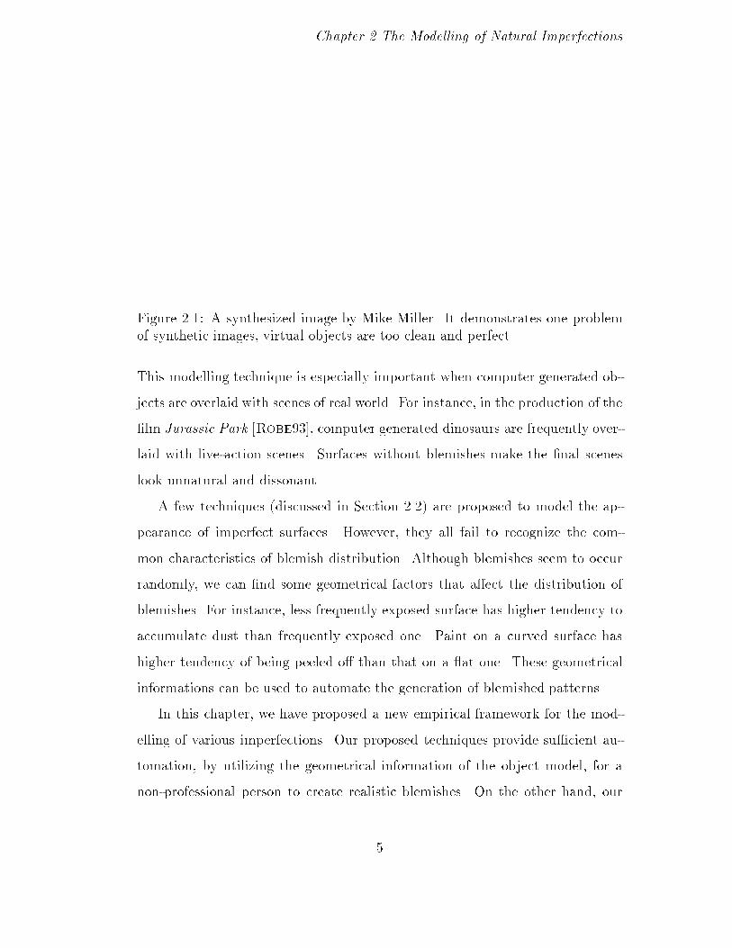
objects and leather objects, etc. Figure 2.5 and 2.6 show two di�erent objects

with chaotic scratch patterns. Both �gures show that scratches usually appear at

places with high surface curvature. Surface exposure also a�ects the formation

of scratches, since less exposed surfaces have less chance of being peeled o� by

any external forces. Notice the leg in the back in Figure 2.5 gets less scratches

than the one in the front.

2.3.3 Rusting

Corrosion is the gradual deterioration of any metal due to its reaction with

air, water or other chemicals to form oxides or other compounds. Rusting is

the term used to describe the corrosion of one speci�c metal, iron. As iron

is the most widely used metal in the world, rusting is the most common type

of corrosion. The necessary condition of rusting is the presence of oxygen and

water. However, there are some factors catalyzing the rusting process. They

are the presence of electrolytes, heat and the presence of another metal, like

copper, tin or silver to be in contact with iron. One way to protect iron from

10


Figure 2.5: Painted chair with scratches.

rusting is to apply a protective layer such as paint, plastic coating, varnish and

grease. Therefore, when the protective layer is peeled o� from the ferric object,

rusting usually occurs. Figure 2.5 shows the reddish brown rust on the scratched

portions of the metallic chair. Since rusting usually appears on the scratched

surface, curvature and surface exposure a�ect the tendency of rusting indirectly.

2.3.4 Mould

Mould [To77] is the result of dispersal of fungi on the surface of organic matter,

such as bread, cheese, and etc. The appearance of mouldy pattern is usually in

the form of aggregates (Figure 2.7) due to the colonization of fungus. Shady,

11


Figure 2.6: Leather bag with scratches.

wet and warm environment favours the growth of fungi. Again, surface exposure

a�ects the formation of mould. Less exposed surface usually has less chance of

being illuminated, hence has a higher tendency of moulding.

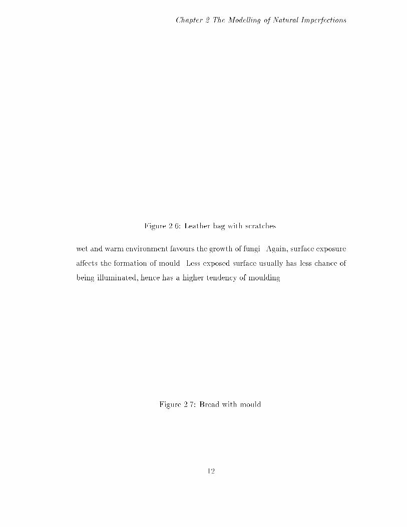
Figure 2.7: Bread with mould.

12


2.4 NewModelling Framework for Natural Im-

perfections

Under the new framework, the modelling process basically consists of 2 phases:

the calculation of tendency value and the generation of chaotic patterns. The

�rst phase involves the determination of a tendency value for each surface point of

interest. Since the distribution of imperfections is usually related to the surface

geometry, we can calculate the tendency value according to these geometrical in-

formations. The tendency value represents the potential of that surface point of

interest to become blemished. In the second phase, we generate chaotic patterns

according to the calculated tendency. The separation of the modelling process

into two phases has an advantage: the generation method of chaotic patterns can

be easily replaced with another method to produces di�erent patterns without

interferring the tendency calculations.

2.4.1 Calculation of Tendency

Sources of Imperfection

The formation process of blemishes is very complex. It may be due to human

factors, physical laws and other unpredictable events. However, we can imagine

that the formation of blemishes is due to di�erent kinds of abstract imperfection

sources. For instance, scratches are usually found near the handle of leather

handbag (Figure 2.6). This is due to frequent contact with human hands. In

this case, we can imagine that there is an abstract scratch source near the

handle. Dust particles are usually accumulating on upward surface due to the

e�ect of one physical law, gravity. We can also imagine that there is a dust

source placed above the surface. This abstraction of imperfection sources is

analogous to the concept of light sources [Fole90, ch. 16] [Watt92, pp. 42{48].

13


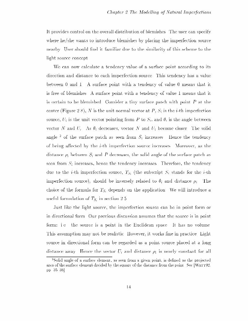
It provides control on the overall distribution of blemishes. The user can specify

where he/she wants to introduce blemishes by placing the imperfection source

nearby. User should �nd it familiar due to the similarity of this scheme to the

light source concept.

We can now calculate a tendency value of a surface point according to its

direction and distance to each imperfection source. This tendency has a value

between 0 and 1. A surface point with a tendency of value 0 means that it

is free of blemishes. A surface point with a tendency of value 1 means that it

is certain to be blemished. Consider a tiny surface patch with point P at the

center (Figure 2.8), N is the unit normal vector at P , Si is the i-th imperfection

source, Ui is the unit vector pointing from P to Si, and �i is the angle between

vector N and Ui. As �i decreases, vector N and Ui become closer. The solid

angle 2 of the surface patch as seen from Si increases. Hence the tendency

of being a�ected by the i-th imperfection source increases. Moreover, as the

distance �i between Si and P decreases, the solid angle of the surface patch as

seen from Si increases, hence the tendency increases. Therefore, the tendency

due to the i-th imperfection source, TSi (the subscript Si stands for the i-th

imperfection source), should be inversely related to �i and distance �i. The

choice of the formula for TSi depends on the application. We will introduce a

useful formulation of TSi in section 2.5.

Just like the light source, the imperfection source can be in point form or

in directional form. Our previous discussion assumes that the source is in point

form: i.e. the source is a point in the Euclidean space. It has no volume.

This assumption may not be realistic. However, it works �ne in practice. Light

source in directional form can be regarded as a point source placed at a long

distance away. Hence the vector Ui and distance �i is nearly constant for all

2Solid angle of a surface element, as seen from a given point, is de�ned as the projected

area of the surface element divided by the square of the distance from the point. See [Watt92,

pp. 35{36]

14


ii

Uθ

N S

P

i

Figure 2.8: A tiny surface patch.

surface points. That is why it is known as directional source. One example of

directional source is the Sun. Since the Sun is far away from the Earth, light rays

from the Sun are basically in parallel. Since �i is now constant, TSi is inversely

related to �i only.

If more than one source is given, we shall sum up the tendency value due to

each source (in point form or directional form). Hence, the overall tendency TS

of a surface point due to all sources is

TS =mXi=1

TSi (2.1)

where m is the total number of imperfection sources and

TSi =

8><>:

TSi(�i; �i) if source is in point form,

TSi(�i) if source is in directional form.

15


External Factors

The tendency value TS calculated using the above formula is a predicted value.

The actual tendency value may deviate from the predicted value due to external

factors. Di�erent kinds of imperfections may be a�ected by di�erent external

factors. Nevertheless, there is one common external factor. It is surface expo-

sure. In this section, we will describe how we can model this geometrical factor.

Notice that other external factors also exist and will be discussed when we apply

the framework to model dust accumulation and scratching in section 2.5 and 2.6.

In general, the actual tendency T for a surface point of interest, after considering

those external factors, is the tendency TS scaled by a function � of all external

factors Ei's.

T = max(0;min(1; T0 + TS � �(E1; E2; E3; : : :))) (2.2)

where Ei is the i-th external factor.

T0 is a constant, s. t. 0 � T0 � 1.

Surface Exposure Consider the intersection of a ray Ri, which is �red from

a surface point P , and an obstacle at distance di from P (Figure 2.9). As

di increases (i.e. the obstacle moves away from point P ), the e�ect of that

obstacle on the surface exposure � at P decreases non-linearly. We de�ne a

weight function ! of di that returns value in [0; 1] s.t. !(d1) � !(d2) if d1 � d2,

!(di) = 0 when di = 0, and !(di) ! 1 when di ! +1 (i.e. no intersection).

This function should be non-linear. We de�ne this function as,

!(di) =di

dh + di

(2.3)

where dh is a user-de�ned constant called the half-exposure distance, which is

roughly the average spacing between the point P and other nearby objects that

would reduce the exposure at point P to 0.5 (Figure 2.10).

16


P

Riid

obstacle

Figure 2.9: Ray Ri intersect with an obstacle.

1

0.5

0dh

di

ω di( )

Figure 2.10: The function !.

17


P

Figure 2.11: n evenly distributed rays emitted from point P .

If we �re many rays from point P and evenly distribute them in the upper

hemisphere of point P (Figure 2.11), the surface exposure � is then de�ned by

the following equation,

� = limn!1

1

n

nXi=1

!(di) (2.4)

� will be 1 when P is completely exposed since all !(di) = 1. � will be 0 when

P touches with any obstacle since all !(di) = 0.

In practice, we can determine � using one-level ray tracing. We subdivide the

surface of the upper hemisphere above point P into several equal sized windows.

For each window, we �re certain amount of rays from point P through the

window to detect whether those rays intersect with any obstacle. Then we can

approximate the surface exposure by

� =1

n0

n0Xi=1

!(di) (2.5)

where n0 is number of rays emitted, n0 is a �nite constant,

!() and di are de�ned as before.

18


This is a sampling technique. The more windows are subdivided and the

more rays are �red, the more accurate the approximation is. However, this

method inherits the same problems as the original ray tracing, namely aliasing

and expensive intersection tests. The aliasing problem can be solved by su-

persampling [Fole90, ch. 14], distribution ray tracing [Cook84], cone tracing

[Aman84] or pencil tracing [Shin87, Shin89]. However, there is no complete

solution to decrease the computational cost of ray tracing to a reasonable level.

A more economic approach to determine � is described in section 2.5.

2.4.2 Generation of Chaotic Pattern

After the �nal tendency value T is calculated, we can generate blemishes ac-

cording to this tendency. Since blemishes are usually in irregular patterns, we

need some stochastic methods to generate such patterns. In this section, we

suggest two standard methods: solid texturing with fractal/noise function, and

rule-guided aggregation.

Solid Texturing with Fractal and Noise Function

Solid texturing [Peac85, Perl85] is an extension of traditional texture map-

ping. Traditional texture mapping maps a 2D texture to the surface of an object.

This mechanism is altered for solid texture. Instead of 2D texture space, solid

texturing uses 3D texture space. For each point of the object to be textured,

there is an associated point in the 3D texture space. The traditional texture

mapping is analogous to wrapping the object with a sheet of paper (2D texture

space). Solid texturing is analogous to carving the object from a piece of mate-

rial, like wood and marble (3D texture space). The advantage of solid texturing

is that there is no distortion during mapping. The 3D texture can be obtained

by creating a 3D lattice of texture values. Mathematical functions can be used

to generate values at the points of the 3D lattice. Two popular functions are

19


fractional Brownian motion and Perlin's noise function.

Mandelbrot observed that many natural objects and phenomena are stochas-

tically self-similar [Mand77, Peit88] which is the main criterion of fractal ob-

jects. Since then, fractal has been successfully used in the generation of di�erent

natural objects, like landscapes [Four82, Mand82, Voss85, Kalr91], plants

[Oppe86, Kalr91] and clouds [Voss85]. One of the fractal functions, fractional

Brownian motion (fBm) [Peit88, pp. 58{70], has been used by many researchers

[Voss88, Saup88, Beck90] to generate interesting chaotic patterns. The origi-

nal fBm, VH(t), is a single valued function of one variable, t (usually time). Its

increment VH(t2)� VH(t1) has a Gaussian distribution with variance

hjVH (t2)� VH(t1)j2i / jt2 � t1j2H

where the brackets h and i denote ensemble averages over many samples of VH(t)

and parameter H has a value between 0 and 1. This fBm can be extended to

accept positional vector as input. The extended version is frequently used as

a solid texturing function. The detailed explanation of fBm can be found in

[Peit88]. We shall not go into detail here.

Perlin [Perl85] proposed another useful stochastic solid texturing function,

noise(), which is a scalar valued function taking a 3D positional vector as input.

It has three major properties:

� Statistical invariance under rotation: it has the same statistical property

even when we rotate its domain.

� Statistical invariance under translation: it gives same statistical charac-

teristic no matter how we translate its domain.

� It has no visible features within a certain narrow size range.

The function noise() is good because it introduces noise e�ect without sacri-

�cing the continuity and the control over spatial frequency. Perlin also derived

20


a turbulence function based on this noise function. He used the noise and tur-

bulence function to generate convincing images of waves and �re.

To generate chaotic patterns, we do the following procedure. Instead of

calculating the whole 3D texture space, we only calculate the noise/fBm function

whenever necessary. When we shade a point on object surface, we �rst calculate

a noise value using fBm() or noise() with a positional vector as input. The

returned noise value is multiplied by the tendency T to create a pattern according

to the tendency. Finally, by mapping di�erent ranges of resultant value to

di�erent colors, we can receive a chaotic pattern. This method is especially

useful in the generation of scratch patterns, rust patterns and fuzzy dust layers.

Rule-guided Aggregation

Becket [Beck90] proposed rule-guided aggregation to generate patterns of stain

and rust. Some sticky seeds are �rst placed on the surface. Then a di�usion

process is performed. During this process, whenever a oating particle collides

with the sticky seed, there is a chance that the particle will stick to the seed.

This possibility is a function of distance between the central seed and the oating

particle. Large distance yields small possibility. When the di�usion process

�nish, aggregation of particles will be formed.

By placing more seeds in the position with a higher tendency value, we can

associate the pattern with our calculated tendency value. Notice that this is a

method to compose the pattern in the texture space. The mapping process may

still introduce distortion.

2.5 Modelling of Dust Accumulation

Dust accumulation is a common natural phenomenon in real life. Modelling of

dust accumulation, however, has not been well studied. We present a technique

21


to model the tendency of dust particles settled on object surface based on the

properties of surface and the geometry of object. The scattering of light by air-

borne dust has been well-studied [Blin82, Max86, Nish87, Rush87] and we

shall not consider it here. We illustrate our techniques with images of synthetic

dusty objects.

2.5.1 Predicted Tendency of Dust Accumulation

Due to the e�ect of gravity, horizontal surfaces usually accumulate more dust

than inclined ones. However, if an object is placed near an open window in

front of a dusty construction site, surfaces facing the window would have more

dust particles accumulated on it than on other faces. Therefore inclination of

a surface against the direction of the dust source (which might be in terms of

the combined e�ect of gravity, wind direction and the actual source of dust

particles) would certainly a�ect the amount of dust particles settled. On the

other hand, this amount is also dependent on the surface type. A sticky surface

(a furry, rough or adhesive one) is more likely to accumulate dust particles than

less-sticky ones (e.g. a smooth one).

Consider the small surface patch in Figure 2.8. Assuming surface properties

are isotropic,3 the predicted tendency of dust accumulation of a surface point

due to a dust source would be a function of �i, the angle between surface normal

and the vector pointing from P to i-th dust source, and �, a stickiness factor

of the surface. Instead of providing a physical model to the dust adhering

process, we adopt some functions that approximate the physical process. The

function should has its peak when �i is 0 and gradually falls o� as �i increases.

Furthermore, an increase in stickiness would decrease the rate of falling o� of

dust particles. These e�ects are very similar to the re ection of light from a

3We say a surface property is isotropic if the surface property is independent of the viewing

direction.

22


ηSi

η

i

=1

=8

Figure 2.12: Predicted tendency functions with di�erent values of �. �i is kept

constant.

surface. The dust source is analogous to the light source. The fall o� in dust

amount as �i increases is similar to the fall o� in di�use component of light

re ection. Therefore it is natural to consider a function similar to Phong's

re ection model [Watt92] to model this predicted tendency function:

TSi =

8><>:

cos�(�i) if source is in directional form,

1

�2i

cos�(�i) if source is in point form.(2.6)

where �i is angle between vector N and Ui,

�i the distance from point P to Si,

� is the surface slippiness (large � means less sticky).

TSi has all the required properties (Figure 2.12): A highly sticky surface

(solid curve in Figure 2.12) accumulates larger total tendency (area under the

curve) than a less sticky one (dashed curve in Figure 2.12). The computation

is also e�cient, cos(�i) is simply the dot product N � Ui. Figure 2.13 shows a

dusty sphere with a directional dust source applied from above using the cosine

function stated before.

23


2.5.2 External Factors

To model the in uence by external factors like coverage or scraping, the predicted

tendency TS is multiplied by a function �, which tells how much the predicted

tendency is realized in the actual environment.

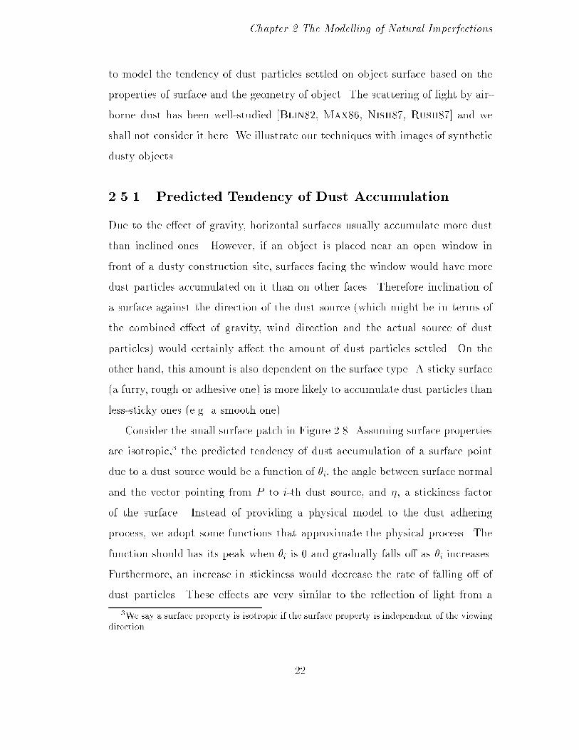
Figure 2.13: A dusty sphere with one directional dust source applied from the

top. � = 1 and � = 1.

Figure 2.14: The same dusty sphere. � = 0:6 and � = 1.

24


Figure 2.13 and 2.14 show a dusty sphere generated by multiplying the pre-

dicted tendency with di�erent �. The value of � is kept constant throughout

the whole surface of the sphere in these two examples. In practice, � varies from

point to point.

The value of � is dependent on the geometry of the object and can be further

in uenced by other factors like coverage and scraping.

Surface Exposure

Consider the object in Figure 2.15. Area B is less exposed to air than area A.

As area B has less exposure than area A, the dust amount that area B may

receive is less. On the other hand, area B may eventually result in more dust

accumulation - since area B is less exposed, the dust particles accumulated on it

have less chance of being removed by wind or scraping. Hence the dust amount

of area B is larger than that of area A.

A B

Figure 2.15: Object with a portion in 'shadow'.

In order to model both cases, the term � can be written as a function of

surface exposure �.

� =

8><>:

0; �0< 0

�0; 0 � �

0

(2.7)

where �0 = �o � r0� and

�o is a factor modelling the global external e�ects, s.t. �o 2 <.

25


� is the surface exposure, such that 0 � � � 1. Larger value

means more exposed.

r0 is a scaling factor to scale the e�ect of surface exposure and r0 2 <.

When r0 is positive, the surface exposure is negatively related to �. This

models the case that area A accumulates less dust than area B. Figure 2.16

shows one example with negative surface exposure e�ect. When r0 is negative,

the surface exposure is positively related to �. This models the opposite case.

Figure 2.17 shows the same object with positive exposure e�ect.

Figure 2.16: The e�ect of negative surface exposure (i.e. r0 > 0): less-exposed

area received more dust.

We have described in section 2.4.1 a method to determine �. However, it is

expensive to be accurate. We present a more economic approach here. Instead

of �nding an accurate � at each surface point of interest. We can make use of

the fuzzy property of dust layer. We only need a very rough approximation of �

at each surface point by emitting only a few number of rays in random (for the

purpose of anti-aliasing) direction in the upper hemisphere of surface point P .

26


Figure 2.17: The e�ect of positive surface exposure (i.e. r0 < 0): less-exposed

area accumulated less dust.

Then, an inaccurate � can be evaluated by equation 2.5 at each surface point of

interest. Although � is inaccurate in the microscopic level, it is accurate in the

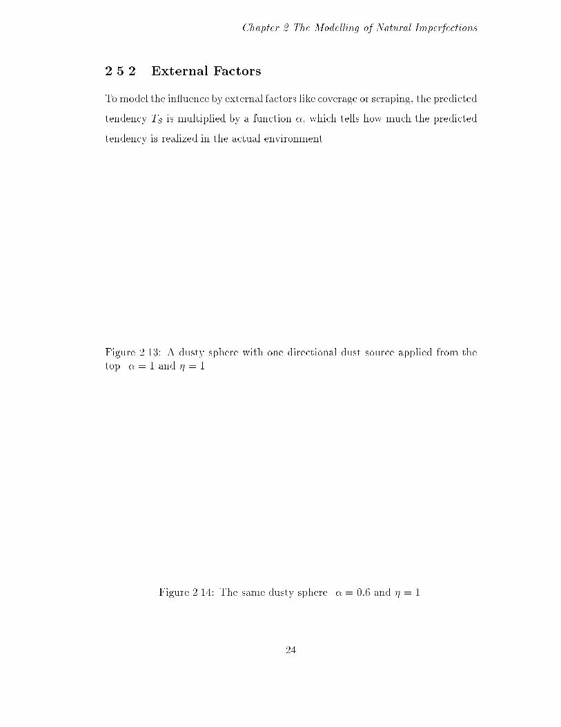
macroscopic level (i.e. on average). This can be shown by Figure 2.18 and 2.19,

which are generated using 1 and 5 random rays respectively. The value of surface

exposure would have a greater variation, if fewer rays are emitted. This would

also result in a more scattered appearance.

Scraping

E�ects due to scraping are modelled using a dust mapping technique, which is

a variant of texture mapping [Blin76, Heck86]. The surface dust amount is

changed according to the pattern in the dust map, which is just a texture map.

The equation of � is now:

� =

8><>:

0; �0< 0

�0; 0 � �

0

(2.8)

27


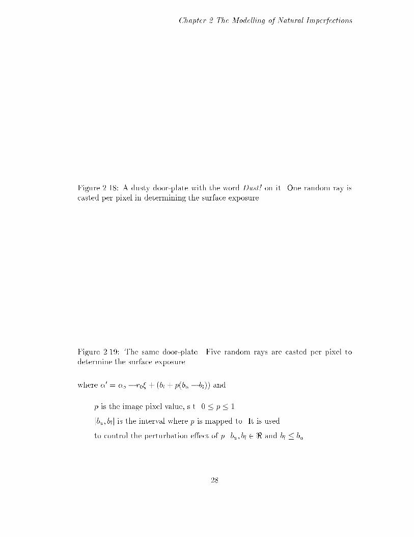
Figure 2.18: A dusty door-plate with the word Dust! on it. One random ray is

casted per pixel in determining the surface exposure.

Figure 2.19: The same door-plate. Five random rays are casted per pixel to

determine the surface exposure.

where �0 = �o � r0� + (bl + p(bu � bl)) and

p is the image pixel value, s.t. 0 � p � 1.

[bu; bl] is the interval where p is mapped to. It is used

to control the perturbation e�ect of p. bu; bl 2 < and bl � bu.

28


Figure 2.20 shows how one speci�c scanline in the dust map (left diagram

in Figure 2.20) perturbs the term � (right diagram in Figure 2.20). Figure 2.21

shows the dust pattern on a sphere modi�ed with the dust map on the left of

Figure 2.20.

x0 x1 x2 x3

x

α

x0 x1 x2 x3

bu

bl

Figure 2.20: The dust map used to perturb the tendency of dust accumulation

on the sphere.

Figure 2.21: The dusty sphere modi�ed with a dust map in the previous �gure.

29


2.5.3 Generation of Fuzzy Dust Layer

It is possible to apply the �nal tendency value T as the thickness parameter

to Blinn's light re ection function [Blin82]. A simpler approach, however, is

adopted in our implementation. The �nal tendency T calculated by equation 2.2

is further perturbed by Perlin's noise function (described in section 2.4.2) to give

a fuzzy appearance. The �nal surface property for rendering are then linearly in-

terpolated with the perturbed value between the original object surface property

and the surface property when the surface is fully covered with dust particles

(see Equation 2.9). The latter is prede�ned. This linear interpolation of surface

property is just a simpli�ed approximation. All synthetic dusty images (Fig-

ure 2.13, 2.14, 2.16, 2.17, 2.18, 2.19, 2.21 and 2.22) are generated using this

simpli�ed approach.

Sfinal = T0Sdust + (1� T

0)Sobject (2.9)

where T 0 = T � noise(P ) and

Sfinal is the �nal surface properties,

Sdust is the surface properties when fully covered with dust,

Sobject is the surface properties when free of dust,

T is the �nal tendency calculated by Equation 2.2,

noise() is the Perlin's noise function which returns value in [0; 1],

P is the positional vector.

A more accurate approach is to precompute an array of BRDF (Bidirectional

Re ectance Distribution Function) tables [Kaji85, West92, Ward92]. Di�er-

ent tables record the BRDF of the surface patch covered with di�erent amount

of dust particles. On rendering, the actual re ectance can be interpolated among

these BRDF tables using the �nal tendency T .

30


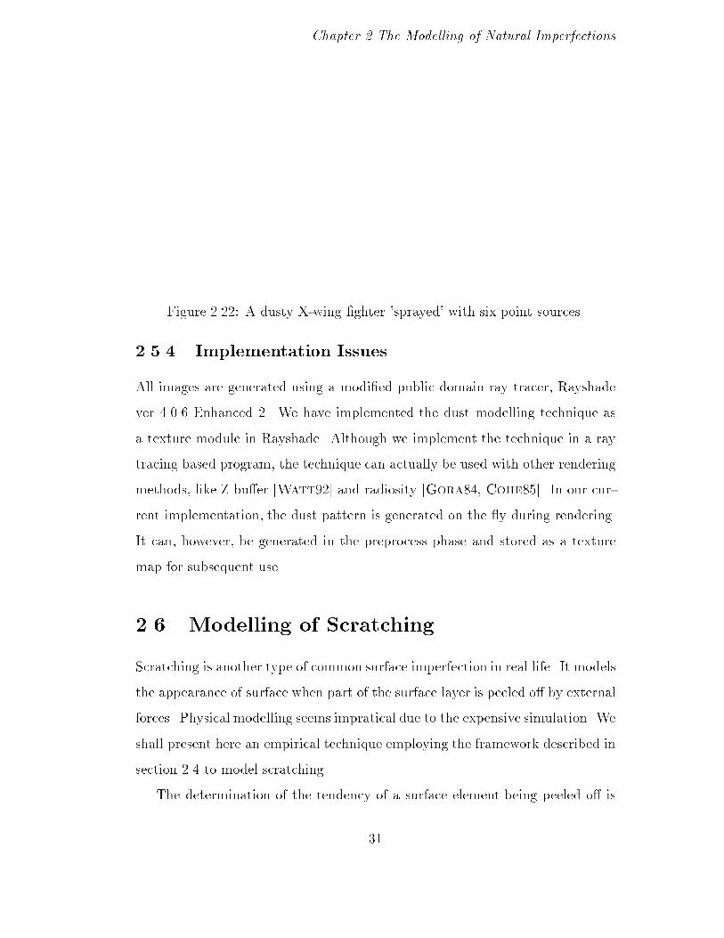
Figure 2.22: A dusty X-wing �ghter 'sprayed' with six point sources.

2.5.4 Implementation Issues

All images are generated using a modi�ed public domain ray tracer, Rayshade

ver 4.0.6 Enhanced 2. We have implemented the dust modelling technique as

a texture module in Rayshade. Although we implement the technique in a ray

tracing based program, the technique can actually be used with other rendering

methods, like Z bu�er [Watt92] and radiosity [Gora84, Cohe85]. In our cur-

rent implementation, the dust pattern is generated on the y during rendering.

It can, however, be generated in the preprocess phase and stored as a texture

map for subsequent use.

2.6 Modelling of Scratching

Scratching is another type of common surface imperfection in real life. It models

the appearance of surface when part of the surface layer is peeled o� by external

forces. Physical modelling seems impratical due to the expensive simulation. We

shall present here an empirical technique employing the framework described in

section 2.4 to model scratching.

The determination of the tendency of a surface element being peeled o� is

31


similar to that of dust accumulation, except that one more external factor takes

place. It is the surface curvature.

Since the calculation of predicted tendency due to a scratch source is sim-

ilar to that of dust accumulation in Section 2.5.1, we shall concentrate on the

discussion of the external factor.

2.6.1 External Factor

The e�ect of surface exposure and scraping is discussed in Section 2.5.2. We

shall not repeat here. In this section, we focus on one factor which is speci�c to

scratching, surface curvature.

Surface Curvature

Paint on a protrusive surface is more likely to be peeled o� than that on a at one.

The scratches usually start from the protrusive area and then propagate to the

surroundings. This is because the protrusive nature increases the chance of being

attacked by external forces. Note that surface exposure alone cannot account

for such e�ect. Consider a convex surface and a at surface (Figure 2.23). Both

of them can be completely exposed, but paint on the convex one has a larger

tendency of being peeled o�.

Figure 2.23: Paint on the convex surface has a larger tendency of being peel o�

than that on a at one, even though they have the same surface exposure.

32


The de�nition of surface curvature is de�ned as follows. Without loss of

generality, we can represent any surface as a parametric surface. For each plane

containing the normal at a particular point P on the surface, the curvature �

of the intersection curve between the plane and the surface at point P can be

determined. As the plane is rotated about the normal, the curvature changes. It

can be showed that there exists distinct directions for which the curvature is a

minimum (�min) and maximum(�max). They are known as principal curvatures.

Two combinations of the principal curvatures are useful, they are the average

curvature H and the Gaussian curvature K.

N

P

Q(u,w)

Figure 2.24: The curvature at surface point P is de�ned as the curvature of the

curve of intersection of the plane containing the normal and surface Q(u;w).

H =�min + �max

2(2.10)

K = �min�max (2.11)

Dill [Dill81] showed that the average curvature and the Gaussian curvature

of a biparametric surface Q(u;w) are,

33


H =AjQwj2 � 2BQu �Qw + CjQuj2

2jQu �Qwj3(2.12)

K =AC �B

2

jQu �Qwj4(2.13)

where

A = (Qu �Qw) �Quu

B = (Qu �Qw) �Quw

C = (Qu �Qw) �Qww

Qu =@Q

@u

Qw =@Q

@w

Quu =@2Q

@u2

Qww =@2Q

@w2

Quw =@2Q

@u@w

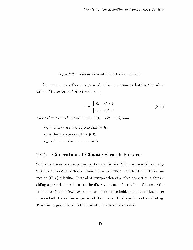
Figure 2.25 and 2.26 show the average and Gaussian curvature values on a

teapot respectively. The red color indicates the surface position is highly curved

while the white color indicates the surface is at.

Figure 2.25: Average curvature on a teapot.

34


Figure 2.26: Gaussian curvature on the same teapot.

Now we can use either average or Gaussian curvature or both in the calcu-

lation of the external factor function �,

� =

8><>:

0; �0< 0

�0; 0 � �

0

(2.14)

where �0 = �o � r0� + r1�a + r2�G + (bl + p(bu � bl)) and

r0, r1 and r2 are scaling constants 2 <,

�a is the average curvature 2 <,

�G is the Gaussian curvature 2 <.

2.6.2 Generation of Chaotic Scratch Patterns

Similar to the generation of dust patterns in Section 2.5.3, we use solid texturing

to generate scratch patterns. However, we use the fractal fractional Brownian

motion (fBm) this time. Instead of interpolation of surface properties, a thresh-

olding approach is used due to the discrete nature of scratches. Whenever the

product of T and fBm exceeds a user-de�ned threshold, the outer surface layer

is peeled o�. Hence the properties of the inner surface layer is used for shading.

This can be generalized to the case of multiple surface layers,

35


Sfinal =

8>>>>>>>>>>>>>>><>>>>>>>>>>>>>>>:

Slayer0

if 0 � T0< �0,

Slayer1

if �0 � T0< �1,

� � �

Slayeri

if �i�1 � T0< �i,

� � �

Slayermif �m�1 � T

0< �m,

(2.15)

where T 0 = T � fBm(P ) and

m+ 1 is the total number of of surface layers,

Sfinal is the �nal surface properties,

Slayeriis the surface properties of the i-th layer below the outermost one Slayer

0,

�i is the user-de�ned threshold for i-th layer, s.t. 0 � �0 � �1 � � � � � �m � 1

T is the �nal tendency calculated by Equation 2.2,

fBm() is the fractional Brownian motion. fBm() returns value in [0; 1],

P is the positional vector.

Figure 2.27 shows a scratched teapot generated by this method. Figure 2.28

shows the same teapot with a point-formed scratch source applied near the

bottom. This teapot has only two surface layers.

2.6.3 Implementation Issues

Surface Representation

A speci�c type of biparametric surface, Bezier surface patches [Roge90], is used

to model object. It is frequently used in computer graphics. It is given by

Q(u;w) =nBXi=0

mBXj=0

Bi;jJnB ;i(u)KmB ;j(w) (2.16)

36


Figure 2.27: A scratched teapot. The Gaussian curvature e�ect is exaggerated

by setting the r2 to a large value and r1 to zero.

Figure 2.28: The scratched teapot with a point form scratch source applied near

the bottom of the teapot.

where

Jn;i(u) =

0B@n

i

1CAui(1� u)

n�i

Km;j(w) =

0B@m

j

1CAw

j(1 �w)m�j

and

nB, mB are one less than the number of vertices in the u and w directions

37


respectively,

Bi;j's are the vertices of the nB �mB control points.

In practice, 4� 4 control points are used to specify one Bezier surface patch.

Bezier surface patch is usually converted to a mesh of polygons before rendering

due to the ine�ciency of direct rendering of Bezier patch. Recursive subdi-

vision [Lane80] and forward di�erencing [Wall90] are two common methods

to subdivide a Bezier patch into polygons. In our implementation, we use for-

ward di�erencing to subdivide patches into triangles, since it is more e�cient

asymptotically.

Curvature Interpolation

In order to speed up the calculation of curvature, we do not calculate the curva-

ture at every surface point. We calculate the average and Gaussian curvatures

only at the vertices of each subdivided polygon. The curvature values of the

interior points within the polygon are approximated by interpolating among the

curvatures at vertices. This is similar to the case of Gouraud shading [Gour71]

which interpolates the intensities and the case of Phong shading [Phon75] which

interpolates the surface normals. Although this approximation may not be ac-

curate, it is su�cient for our purpose.

Rendering

We also implement the method in the ray tracer, Rayshade 4.0.6 Enhanced 2, as

a texture module. Just like the modelling of dust accumulation, the scratch pat-

tern is generated on the y during rendering. However, the scratch pattern can

be generated in the preprocess phase and stored as a texture map for subsequent

use.

38

Chapter 3

An Improved Space Filling

Curve Halftoning Technique

3.1 Introduction

Some classical halftoning techniques, like ordered dither [Baye73], error di�u-

sion [Floy76] and dot di�usion [Knut87] introduce artifacts into the resultant

bilevel image. Figure 3.10(b) shows the noticeable regular patterns introduced

by ordered dither. Figure 3.10(c) shows the snake-like patterns created by error

di�usion. Figure 3.10(d) shows the dot patterns introduced by dot di�usion.

These artifacts look not just unpleasant, but also misleading to the viewer.

Many newer techniques [Witt82, Ulic87, Geis90, Geis93, Velh91] have been

proposed to reduce these artifacts.

Another important problem in digital halftoning is the deviation from the

ideal intensity due to the smudging of printed dots. This problem is especially

important in high resolution printing. While one can correct this by determining

the transfer function of a particular device through calibration [Goer87], a

better halftoning method could provide a wider range of intensities. Moreover,

the accuracy of the transfer function depends on the consistency of the printing

39

Chapter 3 An Improved Space Filling Curve Halftoning Technique

conditions, e.g. quality of the paper used, type of the ink, etc. This method may

be inaccurate when, for example, the printer is running out of ink, or paper with

di�erent degree of absorbability is used. By clustering the printing dots, we can

reduce perimeters of blackened regions which are roughly proportional to the

smudging error. Hence it is a more reliable means to ensure the dithered images

to have better quality. The traditional ordered dither, Knuth's smooth dot

di�usion [Knut87] and the clustered-dot space �lling curve halftoning method

proposed by Velho and Gomes [Velh91] all have the clustering capability.

Most digital halftoning techniques can either reduce artifacts or reduce print-

ing smudge error, but not both. The clustered-dot space �lling curve halftoning

method can, however, reduce both artifacts and printing smudge error. The

space �lling curve halftoning method is attractive because of its pleasant smooth

grains in the resultant image and the aperiodicity of the halftone pattern. The

clustering ability of the algorithm, hence the amount of smudging, can also be

controlled by a single parameter.

Clustering the dots in the clustered-dot space �lling curve method would

however excessively blur the image. We propose two improvements, selective

precipitation and adaptive clustering, to the clustered-dot space �lling curve

halftoning method. Results from improved method are compared with the im-

ages dithered by clustered-dot space �lling curve method and other popular

halftoning techniques.

Besides comparing these results subjectively, we also compared the quality

of halftone images based on a Gibbs measure [Geis93] and the total length of

perimeters of the blackened areas, which gives a rough measure to the potential

amount of smudging. We use them as the objective measures of the halftone

quality of various methods.

40


3.2 Review on Some Halftoning Techniques

On the subject of digital halftoning, much has been written in the past. Or-

dered dither [Baye73], error di�usion [Floy76] and other coloured noise based

techniques [Geis90, Ulic87], dot di�usion [Knut87] and the more recent space

�lling curve based techniques [Witt82, Velh91, Zhan93] are some of the more

well-known techniques.

3.2.1 Ordered Dither

Ordered dither [Baye73] is probably the most commonly used algorithm. The

basic algorithm is to tile the whole image with a dither matrix D of threshold

values, say

D =

2666666664

19=32 25=32 27=32 31=32

21=32 5=32 3=32 17=32

23=32 7=32 1=32 15=32

29=32 9=32 11=32 13=32

3777777775

Whenever the pixel value (range from 0 to 1, 0 is white, 1 is black) in the

original image exceeds the corresponding threshold value, a corresponding pixel

in the dithered image will be turned on (value 1).

Its popularity is due to the simplicity of the algorithm and its exibility

in being able to produce various halftone screen e�ects at various angles and

densities by simply changing the dither matrix. Another important advantage

o�ered by the method is its ability to cluster the black dots so that the e�ect of

ink smudging can be reduced. Moreover, it can be implemented in parallel. Fur-

thermore, high frequency features in the original image can usually be preserved

thus allowing sharp edges to remain sharp in the halftone image. However, the

technique tends to smooth out the subtle low frequency details. The halftone

resulted also su�ers from a correlated periodicity which would produce clear

gray level bands on a smooth gray ramp (Figure 3.17(a)).

41


3.2.2 Error Di�usion and Dither with Blue Noise

Error di�usion [Floy76] is an elegant scheme designed to preserve the local av-

erage gray level in the halftone image. The method distributes the quantization

error in a pixel to its neighbourhood so that the quantization error in one pixel

would compensate for that arised in another one. Each pixel propagates the

error to its right, lower left, below and lower right neighbours in a �xed ratio.

Here is the pseudocode,

for i = 1 to n

begin

for j = 1 to n

begin

if input[i,j] < 0.5

begin

output[i,j] = 0

end

else

begin

output[i,j] = 1

end

error = input[i,j] - output[i,j]

input[i,j+1] = input[i,j+1] + (error * 7/16)

input[i+1,j-1] = input[i+1,j-1] + (error * 3/16)

input[i+1,j] = input[i+1,j] + (error * 5/16)

input[i+1,j+1] = input[i+1,j+1] + (error * 1/16)

end

end

The variables input and output are 2D arrays holding the original grayscale

image and the dithered image respectively. The pixel value is between 0 and 1.

The variable error contains the propagated error.

One problem with the original error di�usion method is that the �xed error

propagation pattern (or error �lter) would produce annoying visual artifacts

on at areas or on smoothly changing gray ramps. By introducing a certain

degree of randomness into the error propagation ratio and by alternating the

42


raster scanning direction on di�erent scanlines, this artifact can generally be

eliminated. These modi�ed schemes with randomness are classi�ed as blue noise

(high frequency white noise) halftoning methods [Ulic87]. Blue noise methods

produce patterns that are aperiodic and radially symmetrical. Because the low

frequency components are not present, the resulting image would only appear

smooth when viewed from a reasonable distance.

However, the fatal problem with these methods is that they produce dis-

persed dots which tend to smudge and darken the �nal image excessively when

printed on high resolution devices (Figure 3.16(b) and 3.17(b)).

3.2.3 Dot Di�usion

Knuth [Knut87] combines ordered dither and error di�usion to develop the dot

di�usion method. It has both the clustering ability of ordered dither and the

error propagation ability of the error di�usion scheme. The technique has the

additional advantage of being able to run in parallel. However, due to the �xed

di�usion pattern within a cluster, periodic regular patterns are present in the

resultant halftone image (Figure 3.10(d)).

3.2.4 Halftoning Along Space Filling Traversal

A space �lling curve traversal is a continuous trace that passes through all

pixels in the image exactly once. It was �rst discovered by Peano in 1890.

Some classic space �lling curves are the Peano curve (Figure 3.1), the Hilbert

curve (Figure 3.2) and the Sierpinski curve. In 1982, Witten and Neal [Witt82]

proposed a halftoning algorithm based on space �lling curves traversal. The

algorithm traverses the whole gray scale image along a space �lling curve. The

Hilbert curve is particularly suitable for use in halftoning for its higher spatial

coherence compared with the other two [Voor91].

The basic idea of the algorithm is to perform error di�usion along the space

43


Figure 3.1: Traversing an image along a Peano Curve.

Figure 3.2: Traversing an image along a Hilbert curve.

44


�lling curve. Instead of propagating the quantization error in a pixel to 4 neigh-

bour pixels as in original error di�usion, the error is transferred to the next pixel

on the path. Just as error di�usion, the algorithm su�ers from the smudging

problem due to its dispersed-dot property.

Velho and Gomes proposed a clustered-dot version [Velh91] in 1991. As the

program traverses the image, it accumulates pixel values. Whenever a certain

�xed number of pixels, which form a cluster, have been scanned through, the

program generates a number of black dots according to the accumulated gray

value in this cluster. According to the original pseudocode in their paper, the

black dots are always precipitated at the beginning of each cluster. The error

between the actual accumulated gray value and the intensity of generated black

pixels is propagated to the next cluster. The pseudocode is,

Given: The size of cluster is N.

select a space �lling curve path

accumulator = 0

while there is pixel to process

begin

move forward N pixels along the path

move backward N pixels and accumulate gray value

move forward N pixels and generate dots:

if accumulator >= 1

begin

accumulator = accumulator - 1

output pixel is on

end

else

begin

output pixel is o�

end

end

45


The clustered-dot version uses the parameter cluster size, N, to control the

smudging error. As the cluster size increases, more black dots are connected

due to the intertwined nature of space �lling curves (Figure 3.1 and 3.2), the

total perimeter of blackened area decreases, hence reducing the printing smudge

error which depends on the total perimeter. Witten's original algorithm is just

a special case when the cluster size is equal to one pixel.

Figure 3.11(a) and 3.11(b) are the same cat image dithered by space �lling

curve halftoning method with cluster sizes of 1 pixel (i.e. no clustering) and 9

pixels respectively. Both images are free from having periodic regular patterns.

One problem with space �lling curve halftoning techniques is that the curve

may not �t the dither image. For instances, Hilbert curve traverses image with

resolution 2n � 2n, Peano curve traverses image of 3n � 3n. Cole [Cole90]

generalizes the Peano curve and developed murray curves. Murray curve �ts

image with resolution m� n, such that m and n are odd and can be factorized.

Wyvill and McNaughton [Wyvi91] further extend murray curve to develop Geo�

curve which can �t image with width and height both greater than seven.

Clustering minimizes the image darkening problem due to smudging of printed

dots and dot gain. However, as the cluster size increases, the dithered image

becomes blurrier and small details are lost (Figure 3.11(b), 3.12(b), 3.13(b) and

3.14(b)).

3.2.5 Space Di�usion

Space di�usion [Zhan93] is a recently proposed scheme based on Knuth's idea of

dot di�usion but using a space �lling curve pattern to perform the dot di�usion.

The method is identical to Knuth's but with a di�erent di�usion matrix. The

method has the same advantages of being parallel and that no regular periodic

pattern would appear on the resultant images. However, the technique as de-

scribed in the paper no longer have the clustering capability of the clustered-dot

46


space �lling curve method and hence is unsuitable for high resolution printing.

If a clustering scheme similar to the clustered-dot space �lling curve version is

used, the method would su�er from the same excessive blurring problem.

3.3 Improvements on the Clustered-Dot Space

Filling Halftoning Method

One disadvantage of the clustered-dot space �lling curve halftoning method is

that images dithered by this method are usually blurrier than those dithered

by other halftone techniques like ordered dither and error di�usion. One can

improve the quality of dither image by preprocessing the original grayscale im-

age [Ulic87]. Such preprocessing techniques include sharpening, smoothing,

increasing contrast and gamma correction. However, all these methods change

the gray value of each pixel in the original grayscale image, hence producing

unfaithful resultant images. Preprocessing the grayscale image does not solve

the underlying problems in the clustered-dot space �lling halftoning method.

We recognize that the blurring is due to the poor precipitation scheme of black

pixels and the �xation of cluster size in the original method. Aiming at these

two causes, we are proposing two improvements on the clustered-dot space �lling

curve halftoning method, namely, selective precipitation and adaptive clustering.

3.3.1 Selective Precipitation

The clustered-dot space �lling curve halftoning algorithm (Section 3.2.4) precip-

itates the black pixels at a �xed location, say, at the beginning of each cluster.

This results in a poor approximation (Figure 3.3(b)) to the original image when

the original gray values (Figure 3.3(a)) in a particular cluster are not gathered

around that �xed location. Although Velho and Gomes had brie y suggested

in their paper that the white subregion can be centred at the pixel with the

47


highest intensity in order to preserve details, this may still result in a poor

approximation (Figure 3.4(b)).

b. Original Dithering Result

a. Grayscale Image Pixels

c. After Selective Precipitation

Figure 3.3: (a) A straightened cluster along a space �lling curve in the original

gray scale image. (b) Resulting halftone based on the clustered-dot space �lling

curve halftoning method if we precipitate black pixels at the beginning of the

cluster. (c) A better approximation.

b. Velho and Gomes suggestion


c. After Selective Precipitation

Figure 3.4: (a) A straightened cluster along a space �lling curve in the original

grayscale image. (b) Result based on Velho and Gomes's suggestion. (c) Result

using selective precipitation.

We propose a method of selectively placing the output black pixels over the

area with the highest total gray value. This would give a better approximation to

the original gray value distribution. We call this technique selective precipitation.

The algorithm is as follows. The number of black pixels to be output in the

current cluster is determined in the same way as the clustered-dot space �lling

48


curve method. This number is then used as the length of a moving window

which shifts within the halftone cluster. The gray values of the grayscale image

pixels within the moving window are summed and recorded with the position of

the window. Our objective is to �nd the position in the cluster such that the

sum of gray values of bgraysumc consecutive pixels is the highest. That position

is where we start to precipitate the black dots. The algorithm is sketched below:

Assumptions:

1. Assume the pixel has gray value between 0 and 1.

2. In order to simplify the formulation, we number each image pixel in the

order of the space �lling curve traversal. We can reference any pixel on

the original image using the notation input[i] just like an one dimension

array.

Input:

1. clusterstart is the index number of the �rst element of the current clus-

ter.

2. graysum is the sum of gray value inside the current cluster.

3. clustersize is the size of the cluster.

Output:

1. The quantization error is returned through the variable graysum.

Algorithm:

winlen = bgraysumcgraysum = graysum - winlen

winsum = maxsum = 0

winstart = clusterstart

for i = winstart to (winstart+winlen-1)

begin

winsum = winsum + input[i]

end

while (winstart+winlen) - clusterstart < clustersize

begin

if maxsum < winsum

begin

49


maxsum = winsum

rightplace = winstart

end

winsum = winsum - input[winstart] + input[winstart+winlen]

winstart = winstart + 1

end

Output winlen number of black pixels starting from rightplace

The variable input is an array holding the gray values of the original image

pixels. After running the above process, we can output black dots starting from

rightplace. The time complexity of this process is linear since each pixel inside

the cluster is accessed at most twice.

The improvement over the clustered-dot space �lling curve method is quite

substantial. Figure 3.11(c) shows the result of halftoning the cat image using

the improved space �lling curve method with selective precipitation (cluster size

is 9 pixels). Comparing to Figure 3.11(b) which uses the clustered-dot space

�lling curve method (cluster size is also 9 pixels), our image seems sharper and

more subtle details are perceivable. Notice that patterns on the cat's cheeks

can be now seen clearly which are blurred in Figure 3.11(b). Similar improve-

ments can be observed in Figure 3.12(c), 3.13(c) and 3.14(c). All of them seem

sharper and preserve more details which are blurred in the images dithered by

the clustered-dot space �lling curve method. Another e�ect resulted from the

selective precipitation technique is that the e�ective cluster size is usually higher.

This is because when a cluster boundary overlaps a darker area in the original

image, the resultant black dots in clusters on both sides of the cluster bound-

ary would stick to the boundary. In the clustered-dot space �lling method, this

could never happen however.

3.3.2 Adaptive Clustering

50


(a) (b)

(c) (d)

Figure 3.5: (a) Gray scale image of a cross. (b) Dithered by the space �lling

curve with cluster size = 9 pixels. (c) With selective precipitation. (d) After

adaptive clustering with threshold T = 0.012.

Even with selective precipitation, we still cannot ensure that the sharp-

ness of high frequency edges are preserved. Figure 3.5(a) shows an original

grayscale image of a cross with very sharp edges. If we dither this image using

the clustered-dot space �lling curve halftoning method with 9-pixel clusters, we

51


get Figure 3.5(b), which is blurred excessively. The blurring is reduced (Fig-

ure 3.5(c)) on using selective precipitation. However, one can still see that some

edges are still a little bit fuzzy. This example shows that rigid positioning of

black pixels is not the only cause of the blurring.

Another factor which causes the blurring is the rigid grouping of output black

pixels. Figure 3.6 shows the case. The original gray values are accumulated on

both ends of the cluster. In such a case, the only thing selective precipitation

can do is to generate black pixels on the end with higher total gray value.

If we divide the cluster into 2 smaller subclusters however and perform the

selective precipitation process in both subclusters, a better approximation can

be resulted.

b. After Selective Precipitation

c. Cutting the cluster into 2 parts


Figure 3.6: (a) The straightened cluster along the space �lling curve in the

original gray scale image. (b) The result after running the selective precipitation.

(c) better result if the cluster is divided into 2 smaller clusters.

Of course one can decrease the size of all clusters to reduce the occurrence

of the cases as in Figure 3.6(a). However, a smaller cluster size also means a

weaker capability of reducing the e�ect of printer smudge. This is a dilemma. To

make a trade-o�, we use smaller clusters only when necessary. That is, instead

of using a �xed cluster size as in the clustered-dot space �lling curve method,

we allow the cluster size to vary.

One way to decide where to subdivide the cluster is to detect whether the

52


case like Figure 3.6(a) occurs. Instead, we decide to subdivide a cluster wherever

a sharp edge is detected. Since human eyes are more sensitive to high frequency

changes, blurring phenomena on sharp edges are more noticeable (Figure 3.5(c)).

This partitioning of clusters at sharp edges would be able to preserve sharp

details. We call this subdivision technique adaptive clustering.

Figure 3.7: 2D edge detector may detect edge which is not intercepted by the

space �lling curve.

Even though a 2D edge detection �lter can be applied to the image to identify

edges, it is computationally expensive. Furthermore, edges which would not be

intercepted by the space �lling curve (e.g. tangential to the space �lling curve

or at the cluster boundary, see Figure 3.7) would also be detected which are

unnecessary. Since the space �lling curve visits all pixels in the image exactly

once, it e�ectively scales down the 2D image into a 1D chain of signal. It is

good enough to employ just a 1D �lter along the space �lling curve. We �nd

that detecting edges using 1D �lter is good enough for visual purpose. It may

be due to the intertwined behaviour of space �lling curve. This argument can be

shown in all example images (Figure 3.11(d), 3.12(d), 3.13(d), 3.14(d), 3.15(c)

and 3.15(d)) in this thesis. The standard 1D Laplacian of the Gaussian �lter

[Jain89] (Figure 3.8) is applied to this chain of signals to recognize sharp edges.

53


This �lter is the negation of the second derivative of the Gaussian function with

respect to the input signal x:

e

�x2

2�2

�3

p2�

(1� x2

�2)

where � is the standard deviation.

In our implementation, the �lter kernel has a width of 7 pixels. In order to

convolve the �lter on previous and next three pixels (total 7 pixels), we set � to

1.

-0.1

0

0.1

0.2

0.3

-3 -2 -1 0 1 2 3

Negative of Laplacian of Gaussian Filter

Figure 3.8: 1D Negative of the Laplacian of the Gaussian �lter.

The algorithm to perform adaptive clustering is as follows. The image pixels

are scanned through in the original space �lling order. A cluster is formed

whenever N (the maximum cluster size) pixels have been traversed or a sharp

edge is encountered, whichever comes earlier. Selective precipitation is then

performed within the cluster. The pseudocode is shown below:

54


Given:

1. maximum cluster size N,

2. threshold T.

Algorithm:

select a space �lling curve pattern

graysum = 0

clustersize = 0

current = clusterstart = 0

while current < no. of pixel

begin

currconv = result of convoluting the negative of

the Laplacian of the Gaussian �lter

to the image input[] with

input[current] (current pixel)

as the centre.

graysum = graysum + input[current]

clustersize = clustersize + 1

if abs(currconv-lastconv)>T or clustersize>N

begin

perform selective precipitation with parameters

graysum, clustersize and clusterstart.

clustersize = 0

clusterstart = current

end

lastconv = currconv

current = current + 1

end

Figure 3.5(d) shows the cross dithered by this improved �lling curve method

(with adaptive clustering and selective precipitation). The maximumcluster size

N is set to 9 pixels. Our new algorithm completely eliminates all blurring of sharp

edges in this example. There are more samples produced by our algorithm with

N=9 and T=0.012, they are Figure 3.11(d), 3.12(d), 3.13(d) and 3.14(d). Notice

those small details in the background of F16 factory image (Figure 3.13(d)) can

be seen quite clearly. All of them retain sharp edges that would have been blurred

55


using selective precipitation alone. They look sharper than the corresponding

images produced by the clustered-dot space �lling curve halftoning method.

Moreover, the algorithm would not break clusters into subclusters when the

image contains only gradual intensity change, hence maximizing the clustering

capability.

T

T

T

T

InputSignal

ConvolutionResult

Figure 3.9: The upper curve is the 1D input gray scale image signal. The lower

curve is the corresponding convolution result after applying the 1D negative of

the Laplacian of Gaussian �lter.

The sensitivity of the edge detection �lter also a�ects the resulting halftone

image. We control this with a user-de�ned threshold T (Figure 3.9). This value

can also be determined automatically using the technique presented in [Schl91].

A lower threshold would allow more edges to be detected and results in poten-

tially smaller cluster sizes. The e�ect is demonstrated in Figure 3.15.

56


Figure 3.15(a) is the teapot image dithered by the clustered-dot space �lling

curve method with a 55-pixel cluster. Figure 3.15(b), 3.15(c) and 3.15(d) are

images dithered by our improved algorithm using T=100, T=0.08 and T=0.012

respectively. All of them use a maximum cluster size N of 55 pixels. The smaller

the T is, the more edges are detected. Hence more small details are visible.

3.4 Comparison With Other Methods

The resultant halftone images created using various methods are shown in Fig-

ure 3.11{3.17. The quality improvement resulted from our enhanced methods is

promising.

3.4.1 Low Resolution Observations

Figure 3.10 and Figure 3.11 show dithered images of a cat using various halfton-

ing methods. Images produced by ordered dither (Figure 3.10)(b), original error

di�usion (Figure 3.10(c)) and dot di�usion (Figure 3.10(d)) all produced some

forms of artifacts. Ordered dither and dot di�usion generate periodic regular

patterns, while error di�usion produces snake-like patterns. On the other hand,

images dithered by space �lling curve halftoning methods reduce artifacts. Fig-

ure 3.11(a) is dithered using dispersed-dot space �lling curve halftoning method

(cluster size = 1 pixel), while Figure 3.11(b) is dithered by clustered-dot space

�lling curve halftoning method with cluster size = 9 pixels. One can notice

that the image dithered by large cluster is excessively blurred. Notice that the

tongue, the ear, the detail on the forehead and the whisker in Figure 3.11(b) can-

not be seen clearly. Images dithered by both selective precipitation and adaptive

clustering preserve more details than those dithered with selective precipitation

alone. This argument is veri�ed by Figure 3.13(d), where the original grayscale

contains many small details.

57


3.4.2 High Resolution Printing Results

Figure 3.16 and 3.17 show results of printing on a 600 dpi printer. The halftone

images are created respectively using ordered dither (order 4�4), error di�usion,

the clustered-dot space �lling curve method (N=15) and our improved version

with both adaptive clustering and selective precipitation (N=15, T=0.012). The

quality of our images is clearly superior than the clustered-dot space �lling curve

method and more subtle details that are smoothed out in the ordered dither

version are also visible.

The excessive darkening of images by error di�usion is apparent from these

outputs. The artifact of using ordered dither to distribute the errors is also

demonstrated by the appearance of clear bands (false contours) on the gray

scale ramp in Figure 3.17(a).

3.4.3 Analytical Comparison

Gibbs Model

Geist proposes the use of a maximum-entropy Gibbs measure as an objective

indicator of the quality of dithered images. The mathematical details can be

found in [Geis93]. We do not go into the detailed derivations, but present only

how the measure is calculated.

For each pixel, we calculate two terms. The �rst term represents the correla-

tion between the individual dithered pixel and the underlying grayscale intensity.

It is formulated as (1 � 2wi)(2Vi � 1), where Vi is the gray value of the pixel

in the original grayscale image and wi is the dithered pixel with value 0 or 1.

The second term represents the correlation of the neighbourhood of the dithered

pixel and the neighbourhood of the corresponding grayscale pixel. This term is

formulated as f(i; j)(1� 2wi)(1� 2wj) where i is the current dithered pixel and

j is its neighbour. Geist suggested that pixels inside a circle of radius 5 pixels of

58


the current pixel are considered as neighbours. The computational energy E(�)

of a dithered image is the sum of above two terms of all pixels. Hence it is,

E(�) = �n�1Xi=0

�iIi �1

2(n�1Xi=0

n�1Xj=0

Tij�i�j)

where

Tij = Tji =

8><>:�f(i; j) if i, j are neighbors,

0 otherwise.

Ii = (2Vi � 1) (3.1)

�i = (2wi � 1) (3.2)

We have measured results generated by our improved algorithm using the

Gibbs measure. The values E(�) of all dithered images are shown in Table 3.1.

Notice that the more negative E(�) is, the better the quality of the dithered

image is. Among all halftoning algorithm, error di�usion has the lowest energy.

However, it does not have clustering ability. The worst is the ordered dither,

even though it supports clustering.

As the cluster size increases, E(�) increases, hence the quality decreases. In

each of four samples, we get a lower E(�) when we perform selective precipita-

tion. The energy is further lowered when adaptive clustering is also performed.

Among the various space �lling curve based algorithms, our improved method

gives the best results. Moreover, our method performs even better than the

ordered dither, which has clustering ability.

Table 3.2 shows the computational energy when using di�erent threshold T.

As the threshold decreases, the �lter is more sensitive to edges and more edges

are preserved, hence the image quality increases.

Total Perimeter of Black Regions

Another quantity which we have adopted as a measure of the susceptibility to

smudging is the total perimeter of black regions in the dithered image. The

59


Ordered

dithered

(4 � 4

kernel)

Error

di�usion

Dispersed-

dot space

�ll-

ing curve

halftoning

method

(N=1)

Clustered-

dot space

�ll-

ing curve

halftoning

method

(N=9)

Improved

us-

ing selec-

tive pre-

cipitation

(N=9)

Improved

us-

ing selec-

tive pre-

cipitation

and adap-

tive clus-

tering

with

T=0.012

Cat

(Fig. 3.11(a))

-24661 -27206 -26150 -24035 -25398 -26292

F14

(Fig. 3.12(a))

-17164 -21000 -19391 -17145 -18118 -18872

F16 factory

(Fig. 3.13(a))

-22904 -28095 -24978 -16712 -22606 -26472

Teapot

(Fig. 3.14(a))

-17763 -21712 -20178 -17278 -18717 -19143

Table 3.1: Computational energy E(�) of di�erent samples dithered by di�erent

algorithms.

Original space

�lling curve

halftoning

method with

N=55.

Improved with

selec-

tive precipita-

tion and adap-

tive

clustering with

N=55, T=100.

Improved with

selec-

tive precipita-

tion and adap-

tive

clustering with

N=55, T=0.08.

Improved with

selec-

tive precipita-

tion and adap-

tive cluster-

ing with N=55,

T=0.012.

Teapot

(Fig. 3.14(a))

-13317 -16056 -16448 -17513

Table 3.2: Computational energy E(�) of dithered images dithered with di�erent

threshold T.

60


total perimeter is the number of pixel edges between one black and one white

pixel. The smudging error should be roughly proportional to this total perimeter

(The geometry of the perimeter would also a�ect the amount of smudging. We

have not taken into account of this factor for simplicity). The smaller the total

perimeter is, the weaker the e�ect of smudging of printed dots is. Table 3.3 shows

total perimeters of images dithered by various halftoning methods. Among all

samples, error di�usion produces images with the longest total perimeter. This

agrees with the fact that it su�ers from severe smudging (Figure 3.16(b) and

3.17(b)). The best one (smallest total perimeter) is produced by the space �lling

curve method with selective precipitation alone. This is due to the increased

e�ective cluster size as explained in Section 3.3.1. Images dithered by space �ll-

ing curve halftoning method with selective precipitation and adaptive clustering

have longer total perimeter, since some clusters are subdivided. However, these

values are still comparable to values from ordered dither and the clustered-dot

space �lling curve method. This shows that adaptive clustering can generally

improve the image quality without sacri�cing the clustering advantage.

Error

di�usion

Ordered

dither (4�4

kernel)

Original

space �lling

curve

halfton-

ing method

(N=9)

Improved

with selec-

tive precip-

itation only

(N=9)

Improved

with selec-

tive precip-

itation and

adaptive

clustering

with N=9,

T=0.012.

Cat 31052 20780 21594 17700 22344

F14 46918 40398 38975 33958 38124

F16 factory 45157 35826 38795 32913 41239

Teapot 48494 31963 34259 29501 31652

Table 3.3: Total perimeter of di�erent samples dithered by di�erent algorithms.

61


(a) (b)

(c) (d)

Figure 3.10: (a) Original 256�256 gray scale cat. (b) 256�256 Ordered dithered

image applying matrix D. (c) Cat image dithered by error di�usion. (d) Cat

image dithered by dot di�usion.

62


(a) (b)

(c) (d)

Figure 3.11: (a) Dithered by space �lling curve halftoning method with no

clustering (1-pixel cluster). (b) Dithered by space �lling curve halftoning method

with a cluster size N of 9 pixels. (c) Dithered by the same process as previous

�gure, except this image go through an additional selective precipitation process.

(d) Dithered by space �lling curve halftoning method plus selective precipitation

and adaptive clustering with N=9, T=0.012.

63


(a) (b)

(c) (d)

Figure 3.12: (a) 256�256 gray scale image of F14. (b) Dithered by the clustered-

dot space �lling curve halftoning method. The bands on the ground have totally

lost. (c) After selective precipitation process. (d) After selective precipitation

and adaptive clustering with N=9, T=0.012. Notice that the vertical bands on

the ground are clearly visible.

64


(a) (b)

(c) (d)

Figure 3.13: (a) 256 � 256 gray scale image of F16 factory. (b) Dithered by

the clustered-dot space �lling curve halftoning method. (c) After selective pre-

cipitation. (d) After selective precipitation and adaptive clustering with N=9,

T=0.012.

65


(a) (b)

(c) (d)

Figure 3.14: (a) 256 � 256 gray scale image of teapot. (b) Dithered by the

clustered-dot space �lling curve halftoning method. (c) After selective pre-

cipitation. (d) After selective precipitation and adaptive clustering with N=9,

T=0.012.

66


(a) (b)

(c) (d)

Figure 3.15: (a) Dithered by clustered-dot space �lling curve halftoning method

with cluster size=55. (b) Dithered by improved space �lling curve halftoning

method with N=55, T=100. That is detect no edge at all, only selective pre-

cipitation. (c) Dithered by improved space �lling curve halftoning method with

N=55, T=0.08. (d) Dithered by improved space �lling curve halftoning method

with N=55,T=0.012.

67


(a) (b)

(c) (d)

Figure 3.16: The cat image printed on a 600 dpi printer using di�erent halftoning

methods. (a) Ordered dither. (b) Error di�usion. (c) Original space �lling curve

(N=15) (d) Selective precipitation and adaptive clustering (N=15, T=0.012)

(a) (b)

(c) (d)

Figure 3.17: A test image with gradually changing gray values printed on a 600

dpi printer using di�erent halftoning methods. (a) Ordered dither. (b) Error

di�usion. (c) Original space �lling curve (N=15) (d) Selective precipitation and

adaptive clustering (N=15, T=0.012)

68

Chapter 4

Conclusion and Future Work

In this chapter, we draw some conclusions on the two topics discussed previously.

Future works are also stated.

4.1 The Modelling of Natural Imperfections

The use of traditional texture mapping to create the appearance of blemished

surfaces requires a lot of manual adjustment and is di�cult to apply to irreg-

ularly shaped objects. The possible distortions during the mapping process

further complicate the composition of the desired texture. Furthermore, the

distribution of blemishes on di�erent parts of an object cannot be automatically

deduced.

The new framework proposed in this thesis requires only a few parameters

to control the overall e�ect of blemishes. The overall appearance can be con-

trolled by placing a few imperfection sources around the object. Small details

are automatically generated according to geometrical informations. Hence the

user is freed from detail adjustments. The separation of the tendency value

calculation from the generation of the �nal blemish pattern provides the free-

dom to switch pattern generation methods. Solid texturing is used to generate

69

Chapter 4 Conclusion and Future Work

blemished patterns due to its simplicity and e�ciency.

We have applied the framework to the modelling of dust accumulation and

scratching. Some convincing images are resulted. Moreover, the proposed ten-

dency function can be e�ciently computed. This can be seen from our imple-

mentations: we have implemented the model as a texture module of a ray tracer.

Although the tendency value is calculated during rendering, the calculations do

not slow down the rendering process signi�cantly. If the generated patterns are

stored as texture maps for subsequent use, the rendering process can be speed

up further.

As the number of abstract imperfection sources increases, the calculation of

tendency value of each surface point may increase. This may not cause serious

problem because each object usually has a only few private (or local) imperfec-

tion sources associates with it. The imperfection sources of one object cannot

a�ect another object. This is quite di�erent from the case of light source. All

light sources de�ned should be global to all objects in the environment.

In the future, other imperfections, like mould and rust, can be implemented

using the proposed framework. A program that allows placing the imperfection

sources interactively and storing the resultant pattern as texture map is worth

implementing.

To generate more realistic dust patterns, an anisotropic1 re ection model

[Kaji85, Cabr87,Ward92,West92] seems promising. A natural phenomenon

which is quite similar to dust accumulation is snow accumulation. However,

snow has signi�cant volume. The next step we want to take would be to model

precipitations with volume.

1The term anisotropic is opposite to the term isotropic. An anisotropic surface has di�erent

surface properties (e.g. re ection) when it is viewed from di�erent direction.

70

Chapter 4 Conclusion and Future Work

4.2 An Improved Space Filling Curve Halfton-

ing Technique

We have proposed two methods, selective precipitation and adaptive cluster-

ing, to improve the clustered-dot space �lling curve halftoning method. The

images obtained from our improved method appear sharper than that from the

clustered-dot space �lling curve method. The sharpness is achieved without any

form of pre-�ltering. The qualities of the resultant images are also compared

analytically using a Gibbs energy measure and total perimeter of black regions

in the dithered image. These two measures demonstrate that our improved

method does result in better quality halftones without a corresponding increase

in susceptibility to printing smudge.

The improved techniques can be applied to the serial clustered-dot space

�lling curve method as well as the parallel version (space di�usion) proposed by

Zhang [Zhan93].

Our method still inherits some disadvantages of the space �lling curve based

halftoning method. The method requires more memory to store the whole image

due to the irregular traversal of space �lling curve. This can be worked around if

we store pixels of the image in the order of the space �lling curve traversal. This

requires additional conversion from traditional image storing format. Moreover,

a special display method is also required to display the converted images.

Clustering black pixels for output reduces the occurrence of smudging of

printed dots. This is a rather passive approach. It has a disadvantage that

di�erent portion of the imagemay have di�erent intensity error, since the amount

of smudging is di�erent. A more aggressive approach is to compensate the

intensity error due to smudging. We will do more research along this direction

in the future.

71

Bibliography

[Aman84] Amanatides, J. Ray tracing with cones. In Christiansen, H., ed-

itor, Computer Graphics (SIGGRAPH '84 Proceedings), volume 18,

pp. 129{135, July 1984.

[Baye73] Bayer, B. E. An optimum method for two level renditionof

continuous-tone pictures. In Proceedings of the IEEE International

Conference on Communication, pp. 26{11{26{15, 1973.

[Beck90] Becket, W. and Badler, N. I. Imperfection for realistic im-

age synthesis. Journal of Visualization and Computer Animation,

1(1):26{32, Aug. 1990.

[Blin76] Blinn, J. F. and Newell, M. E. Texture and re ection in com-

puter generated images. Communications of the ACM, 19(10):542{

546, October 1976.

[Blin78] Blinn, J. F. Simulation of wrinkled surfaces. In Computer Graphics

(SIGGRAPH '78 Proceedings), volume 12, pp. 286{292, August 1978.

[Blin82] Blinn, J. F. Light re ection functions for simulation of clouds and

dusty surfaces. In Computer Graphics (SIGGRAPH '82 Proceedings),

volume 16, pp. 21{29, July 1982.

72

[Cabr87] Cabral, B., Max, N., and Springmeyer, R. Bidirectional re-

ection functions from surface bump maps. In Computer Graphics

(SIGGRAPH '87 Proceedings), volume 21, pp. 273{281, July 1987.

[Catm74] Catmull, E. E. A Subdivision Algorithm for Computer Display of

Curved Surfaces. PhD thesis, Dept. of CS, U. of Utah, Dec. 1974.

[Cohe85] Cohen, M. A radiosity method for the realistic image synthesis of

complex di�use environments. Master's thesis, Program of Computer

Graphics, Cornell Univ., Aug. 1985.

[Cole90] Cole, A. J. Naive halftoning. In Proceedings of Computer Graphics

International '90, pp. 203{222, 1990.

[Cook84] Cook, R. L., Porter, T., and Carpenter, L. Distributed ray

tracing. In Christiansen, H., editor, Computer Graphics (SIG-

GRAPH '84 Proceedings), volume 18, pp. 137{145, July 1984.

[Dill81] Dill, J. C. An application of color graphics to the display of surface

curvature. In Computer Graphics (SIGGRAPH '81 Proceedings),

volume 15, pp. 153{161, Aug. 1981.

[Floy76] Floyd, R. and Steinberg, L. An adaptive algorithm for spatial

grey scale. In Proceedings of SID 17, pp. 75{77, 1976.

[Fole90] Foley, J. D., van Dam, A., Feiner, S. K., and Hughes, J. F.

Computer Graphics: Principles and Practices (2nd Edition). Addi-

son Wesley, 1990.

[Four82] Fournier, A., Fussell, D., and Carpenter, L. Computer

rendering of stochastic models. In Communications of the ACM,

volume 25, pp. 371{384, June 1982.

73

[Gard84] Gardner, G. Y. Simulation of natural scenes using textured

quadric surfaces. In Christiansen, H., editor, Computer Graphics


[Gard85] Gardner, G. Y. Visual simulation of clouds. In Barsky,

B. A., editor, Computer Graphics (SIGGRAPH '85 Proceedings),

volume 19, pp. 297{303, July 1985.

[Geis90] Geist, R. and Reynolds, R. Colored noise inversion in digital

halftoning. In Proceedings of Graphics Interface '90, pp. 31{38, May

1990.

[Geis93] Geist, R., Reynolds, R., and Suggs, D. A markovian

framework for digital halftoning. ACM Transactions on Graphics,

12(2):136{159, April 1993.

[Goer87] Goertzel, G. and Thompson, G. R. Digital halftoning on the

ibm 4250 printer. IBM Journal Res. Develop., 31(1):2{15, January

1987.

[Gora84] Goral, C. M., Torrance, K. E., Greenberg, D. P., and

Battaile, B. Modeling the interaction of light between di�use

surfaces. In Christiansen, H., editor, Computer Graphics (SIG-


[Gour71] Gouraud, H. Continuous shading of curved surfaces. IEEE Trans-

actions on Computers, C-20(6):623{629, June 1971.

[Gree86] Greene, N. Environment mapping and other applications of world

projections. IEEE Computer Graphics and Applications, 6(11):21{

29, Nov. 1986.

74

[Hanr90] Hanrahan, P. and Haeberli, P. E. Direct WYSIWYG painting

and texturing on 3D shapes. In Baskett, F., editor, Computer

Graphics (SIGGRAPH '90 Proceedings), volume 24, pp. 215{223,

Aug. 1990.

[Heck86] Heckbert, P. S. Survey of texture mapping. IEEE Computer

Graphics and Applications, 6(11):56{67, November 1986.

[Jain89] Jain, A. K. Fundamentals of Digital Image Processing. Prentice

Hall, 1989.

[Kaji85] Kajiya, J. T. Anisotropic re ection models. In Computer Graphics


[Kalr91] Kalra, P. K. Fractals and their applications. In Thalmann,

M. and Thalmann, D., editors, New Trends in Animation and

Visualization, chapter 14, pp. 197{205. John Wiley & Sons, England,

1991.

[Knut87] Knuth, D. E. Digital halftones by dot di�usion. ACM Transactions

on Graphics, 6(4):245{273, 1987.

[Lane80] Lane, J. and Riesenfeld, R. A theoretical development for the

computer generation and display of piecewise polynomial surfaces.

IEEE Trans. Pattern Analysis Machine Intell., 2(1):35{46, 1980.

[Mand77] Mandelbrot, B. B. The Fractal Geometry of Nature. W.H. Free-

man and Co., New York, rev 1977.

[Mand82] Mandelbrot, B. B. Comment on computer rendering of fractal

stochastic models. In Communications of the ACM, volume 25, pp.

581{584, August 1982.

75

[Max86] Max, N. L. Atmospheric illumination and shadows. In Evans,

D. C. and Athay, R. J., editors, Computer Graphics (SIGGRAPH

'86 Proceedings), volume 20, pp. 117{124, Aug. 1986.

[Mill84] Miller, G. S. and Hoffman, C. R. Illumination and re ection

maps: Simulated objects in simulated and real environments. In

SIGGRAPH '84 Advanced Computer Graphics Animation seminar

notes. July 1984.

[Nish87] Nishita, T., Miyawaki, Y., and Nakamae, E. A shading model

for atmospheric scattering considering luminous intensity distribu-

tion of light sources. In Stone, M. C., editor, Computer Graphics


[Oppe86] Oppenheimer, P. E. Real time design and animation of fractal

plants and trees. In Evans, D. C. and Athay, R. J., editors,

Computer Graphics (SIGGRAPH '86 Proceedings), volume 20, pp.

55{64, August 1986.

[Peac85] Peachey, D. R. Solid texturing of complex surfaces. In Barsky,

B. A., editor, Computer Graphics (SIGGRAPH '85 Proceedings),

volume 19, pp. 279{286, July 1985.

[Peit88] Peitgen, H.-O. and Saupe, D. The Science of Fractal Images.

Springer-Verlag, 1988.

[Perl85] Perlin, K. An image synthesizer. In Barsky, B. A., editor,

Computer Graphics (SIGGRAPH '85 Proceedings), volume 19, pp.

287{296, July 1985.

[Phon75] Phong, B.-T. Illumination for computer generated pictures. Com-

munications of the ACM, 18(6):311{317, June 1975.

76

[Robe93] Robertson, B. Dinosaur magic. Computer Graphics World, pp.

44{52, September 1993.

[Roge90] Rogers, D. F. and Adams, J. A. Mathematical Elements for

Computer Graphics. McGraw-Hill, 1990.

[Rush87] Rushmeier, H. E. and Torrance, K. E. The zonal method for

calculating light intensities in the presence of a participating medium.

In Stone, M. C., editor, Computer Graphics (SIGGRAPH '87 Pro-

ceedings), volume 21, pp. 293{302, July 1987.

[Saup88] Saupe, D. Algorithms for random fractals. In Peitgen, H.-O.

and Saupe, D., editors, The Science of Fractal Images, pp. 71{136.

Springer-Verlag, 1988.

[Schl91] Schlag, J. Noise thresholding in edge images. In Graphics Gems

II, pp. 105. Academic Press, 1991.

[Shin87] Shinya, M., Takahashi, T., and Naito, S. Principles and ap-

plications of pencil tracing. In Stone, M. C., editor, Computer

Graphics (SIGGRAPH '87 Proceedings), volume 21, pp. 45{54, July

1987.

[Shin89] Shinya, M., Saito, T., and Takahashi, T. Rendering tech-

niques for transparent objects. In Proceedings of Graphics Interface

'89, pp. 173{82, Toronto, Ontario, June 1989. Canadian Information

Processing Society.

[To77] To, Y. K. Basic Principles in Biology. Hung Fung Book Co. Ltd.,

1977.

[Ulic87] Ulichney, R. Digital Halftoning. MIT Press, 1987.

77

[Upst89] Upstill, S. The Renderman Companion: A Programmer's Guide

to Realistic Computer Graphics. Addison Wesley, 1989.

[Velh91] Velho, L. and Gomes, J. d. Digital halftoning with space �lling

curves. In Sederberg, T. W., editor, Computer Graphics (SIG-


[Voor91] Voorhies, D. Space-�lling curves and a measure of coherence. In

Graphics Gems II, pp. 26{30. Academic Press, 1991.

[Voss85] Voss, R. F. Random fractal forgeries. In Earnshaw, R. A.,

editor, Fundamental Algorithms for Computer Graphics, pp. 805{

835. Springer-Verlag, 1985.

[Voss88] Voss, R. F. Fractals in nature: From characterization to simulation.

In Peitgen, H.-O. and Saupe, D., editors, The Science of Fractal

Images, pp. 22{70. Springer-Verlag, 1988.

[Wall90] Wallis, B. Tutorial on forward di�erencing. In Graphics Gems, pp.

594{603. Academic Press, 1990.

[Ward92] Ward, G. J. Measuring and modeling anisotropic re ection. In

Catmull, E. E., editor, Computer Graphics (SIGGRAPH '92 Pro-

ceedings), volume 26, pp. 265{272, July 1992.

[Watt92] Watt, A. and Watt, M. Advanced Animation and Rendering

Techniques: Theory and Practice. Addison-Wesley Publishing Com-

pany, 1992.

[West92] Westin, S. H., Arvo, J. R., and Torrance, K. E. Predicting

re ectance functions from complex surfaces. In Catmull, E. E., ed-

itor, Computer Graphics (SIGGRAPH '92 Proceedings), volume 26,

pp. 255{264, July 1992.

78

[Witt82] Witten, I. H. and Neal, R. M. Using peano curves for bilevel

display of continuous-tone images. IEEE Computer Graphics and

Applications, 2:47{52, May 1982.

[Wyvi91] Wyvill, G. and McNaughton, C. Three plus �ve makes eight:

A simpli�ed approach to haltoning. In Patrikalakis, N. M., ed-

itor, Scienti�c Visualization of Physical Phenomena (Proceedings of

CG International '91), pp. 379{392. Springer-Verlag, 1991.

[Zhan93] Zhang, Y. and Webber, R. E. Space di�usion: An improved

parallel halftoning technique using space-�lling curves. In Kajiya,

J. T., editor, Computer Graphics (SIGGRAPH '93 Proceedings),

volume 27, pp. 305{312, Aug. 1993.

79

Documents

Fractal Curve Fitting Halftoning Thesis