Embed Size (px)
Citation preview

2009 Spring ME451 - GGZ Page 1Week 12-13: Frequency Response
• We would like to analyze a system property by applying
a test sinusoidal input u(t) and observing a response y(t).
• Steady state response yss(t) (after transient dies out) of a
system to sinusoidal inputs is called frequency
response.
SystemSystem
FR FR –– What is Frequency Response (RF)?What is Frequency Response (RF)?
)(ty)(ty
ss
tAtu ωsin)( =
2009 Spring ME451 - GGZ Page 2Week 12-13: Frequency Response
• RC circuit
• Input a sinusoidal voltage u(t)
• What is the output voltage y(t)?
RR
CC
FR FR –– A Simple Example A Simple Example (1)(1)
)(1
)( sIsC
sY =
)(tu
)()1
()( sIsC
RsU +=
)(ty
1
1)(
+=
RCssG

2009 Spring ME451 - GGZ Page 3Week 12-13: Frequency Response
• TF (R=C=1)
• Let
0 5 10 15 20 25 30 35 40 45 50-1
-0.8
-0.6
-0.4
-0.2
0
0.2
0.4
0.6
0.8
1
r
y
At steadyAt steady--state, state, uu((tt)) and and yy((tt)) has same frequency, has same frequency,
but different amplitude and phase!but different amplitude and phase!
FR FR –– A Simple Example A Simple Example (2)(2)
1
1)(
+=
ssG
ttu sin)( =
uy

2009 Spring ME451 - GGZ Page 4Week 12-13: Frequency Response
• Derivation of y(t)
• Inverse Laplace
0 as t goes to infinity.0 as t goes to infinity.
Partial fraction expansionPartial fraction expansion
(Derivation for general (Derivation for general GG((ss)) is given at the end of lecture slide.)is given at the end of lecture slide.)
FR FR –– A Simple Example A Simple Example (3)(3)
)1
1
1
1(
2
1
1
1
1
1)()()(
22 +
+−+
+=
+⋅
+==
s
s
ssssUsGsY
( )ttety sincos2
1)(
1 +−= −
( ) )45sin(2
1sincos
2
1)(
o
sstttty −=+−=

2009 Spring ME451 - GGZ Page 5Week 12-13: Frequency Response
• How is the steady state output of a linear system when
the input is sinusoidal?
• Steady state output:
– Frequency is same as the input frequency
– Amplitude is that of input (A) multiplied by
– Phase shifts
GainGain
FR FR –– System Response to Sinusoidal InputSystem Response to Sinusoidal Input
)(ty )(tyss
tAtu ωsin)( =)(sG
))(sin()()( ωωω jLGtjGAtyss
+=
ω)( ωjG
)( ωjG∠

2009 Spring ME451 - GGZ Page 6Week 12-13: Frequency Response
• For a stable system G(s), G(jw) (ω is real and positive) is called frequency response function (FRF).
• FRF is a complex number, and thus, has an amplitude and
a phase.
• First order example
ReRe
ImIm
FR FR –– Frequency Response FunctionFrequency Response Function
1
1)(
+=
ssG
−=+∠−∠=∠+
=
− ωωωω
ω
1
2
tan)1()1()(1
1)(
jjG
jG
1
1)(
+=
ωω
jjG

2009 Spring ME451 - GGZ Page 7Week 12-13: Frequency Response
• Second order system
ReRe
ImIm
23
2)(
2 ++=
sssG
ωωωωω
32
2
2)(3)(
2)(
22 jjjjG
+−=
++=
FR FR –– Another FRF ExampleAnother FRF Example
−−=
+−∠−∠=∠
+−=
−
2
1
2
222
2
3tan
)32()2()(
9)2(
2)(
ω
ω
ωωω
ωωω
jjG
jG
ω3j
22 ω−

2009 Spring ME451 - GGZ Page 8Week 12-13: Frequency Response
• FRF
• Two graphs representing FRF
– Bode diagram (Bode plot)
– Nyquist diagram (Nyquist plot)
FR FR –– First Order Example RevisitedFirst Order Example Revisited
1
1)(
+=
ωω
jjG

2009 Spring ME451 - GGZ Page 9Week 12-13: Frequency Response
• Bode diagram consists of gain plot & phase plot
LogLog--scalescale
FR FR –– Body Diagram (Plot) of Body Diagram (Plot) of GG(j(jωω))
(deg) )( ωjG∠
(dB) )(log2010
ωjG
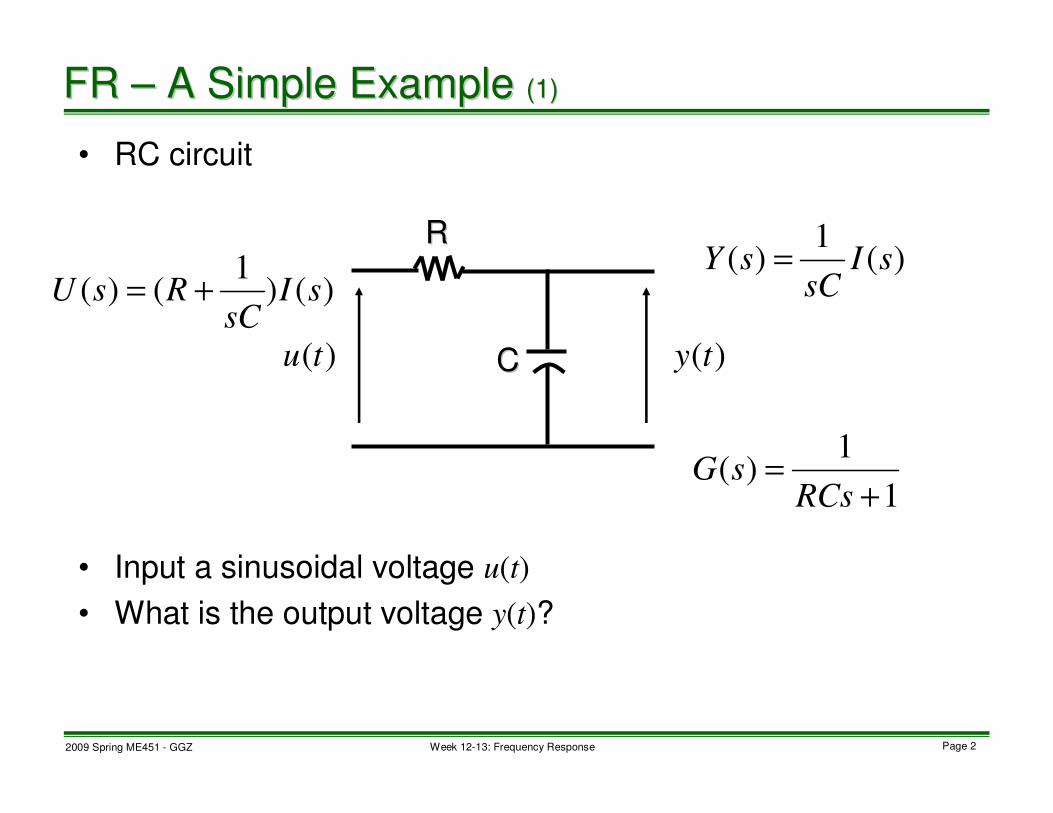
2009 Spring ME451 - GGZ Page 10Week 12-13: Frequency Response
• TF
10-2
10-1
100
101
102
-50
-40
-30
-20
-10
0
10-2
10-1
100
101
102
-100
-80
-60
-40
-20
0
Corner frequencyCorner frequency
FR FR –– Body Diagram of a 1Body Diagram of a 1stst Order SystemOrder System
1
1)(
+=
TssG
<<
>>≈
+=
T
T
TjjG
Tjω
ω
ωω
ω1 if
1 if1
1
1)(
1
T
1
45−
90−
dB/decade20−
1
1)(
+=
ssG

2009 Spring ME451 - GGZ Page 11Week 12-13: Frequency Response
• First order system
FR FR –– Sketching Body DiagramSketching Body Diagram
1
1)(
+=
ssG
11.0
1)(
+=
ssG
110
1)(
+=
ssG

2009 Spring ME451 - GGZ Page 12Week 12-13: Frequency Response
• Bode diagram shows amplification and phase shift of a
system output for sinusoidal inputs with various frequencies.
• It is very useful and important in analysis and design of
control systems.
• The shape of Bode plot contains information of stability, time responses, and much more!
• It can also be used for system identification. (Given FRF
experimental data, obtain a transfer function that matches
the data.)
FR FR –– Remarks on Body DiagramRemarks on Body Diagram
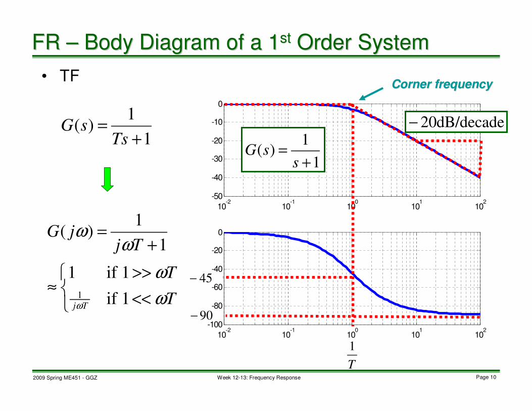
2009 Spring ME451 - GGZ Page 13Week 12-13: Frequency Response
• Sweep frequencies of sinusoidal signals and obtain FRF
data (i.e., gain and phase).
• Select G(s) so that G(jω) fits the FRF data.
Agilent Technologies: FFT Dynamic Signal Analyzer
UnknownUnknown
systemsystem
Generate sin signalsGenerate sin signals
Sweep frequenciesSweep frequencies
Collect FRF dataCollect FRF data
Select Select G(sG(s))
FR FR –– Body Diagram: System IdentificationBody Diagram: System Identification

2009 Spring ME451 - GGZ Page 14Week 12-13: Frequency Response
• Frequency response is a steady state response of
systems to a sinusoidal input.
• For a linear system, sinusoidal input generates
sinusoidal output with same frequency but different amplitude and phase.
• Bode plot is a graphical representation of frequency
response function. (“bode.m”)
• Next, Bode diagram of simple transfer functions
FR FR –– Body Diagram SummaryBody Diagram Summary

2009 Spring ME451 - GGZ Page 15Week 12-13: Frequency Response
Term having denominator of Term having denominator of G(sG(s))
0 as t goes to infinity.0 as t goes to infinity.
FR FR –– Derivation of Frequency ResponseDerivation of Frequency Response
)()()()()( 21
22sC
js
k
js
k
s
AsGsUsGsY
g+
−+
+=
+==
ωωω
ω
==+
−=
−=
−−=
++=
−→
−→
j
jAG
j
AjG
s
AsGjsk
j
jAG
j
AjG
s
AsGjsk
js
js
2
)(
2)()()(lim
2
)(
2)()()(lim
222
221
ω
ω
ωω
ω
ωω
ω
ω
ωω
ω
ωω
ω
ω
4444 34444 21))(sin(
))(())((
2)()(
ωω
ωωωω
ω
jGt
jGtjjGtj
ssj
eejGAty
∠+
∠+−∠+ −=
)}({)( 1
21sCLekekty
g
tjtj −− ++= ωω
2009 Spring ME451 - GGZ Page 16Week 12-13: Frequency Response
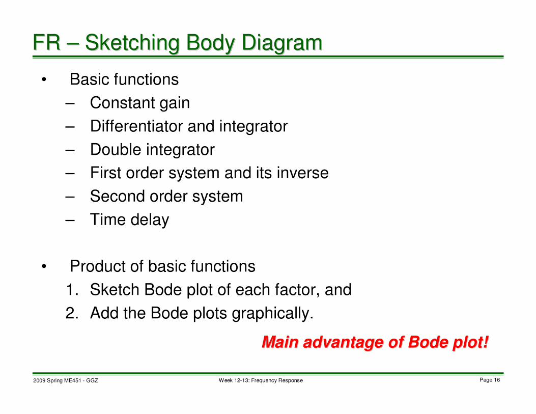
• Basic functions
– Constant gain
– Differentiator and integrator
– Double integrator
– First order system and its inverse
– Second order system
– Time delay
• Product of basic functions
1. Sketch Bode plot of each factor, and
2. Add the Bode plots graphically.
Main advantage of Bode plot!Main advantage of Bode plot!
FR FR –– Sketching Body DiagramSketching Body Diagram

2009 Spring ME451 - GGZ Page 17Week 12-13: Frequency Response
10-2
10-1
100
101
102
19
19.5
20
20.5
21
10-2
10-1
100
101
102
-1
-0.5
0
0.5
1
• TF
FR FR –– Body Diagram (Constant Gain)Body Diagram (Constant Gain)
ωωω ∀=∠=⇒= ,0)( ,)()( ojGKjGKsG
10=K

2009 Spring ME451 - GGZ Page 18Week 12-13: Frequency Response
10-2
10-1
100
101
102
-40
-20
0
20
40
10-2
10-1
100
101
102
89
89.5
90
90.5
91
• TF
FR FR –– Body Diagram (Differentiator)Body Diagram (Differentiator)
ωωωω ∀=∠=⇒= ,90)( ,)()( ojGjGssG
dB/decade20+

2009 Spring ME451 - GGZ Page 19Week 12-13: Frequency Response
• TF
10-2
10-1
100
101
102
-40
-20
0
20
40
10-2
10-1
100
101
102
-91
-90.5
-90
-89.5
-89
Mirror image of Mirror image of
the bode plot of the bode plot of
1/s with respect 1/s with respect
to to ωω--axis.axis.
ωωω
ω ∀−=∠=⇒= ,90)( ,1
)(1
)( ojGjG
ssG
e20dB/decad-
FR FR –– Body Diagram (Integrator)Body Diagram (Integrator)
2009 Spring ME451 - GGZ Page 20Week 12-13: Frequency Response
10-2
10-1
100
101
102
-100
-50
0
50
100
10-2
10-1
100
101
102
-181
-180.5
-180
-179.5
-179
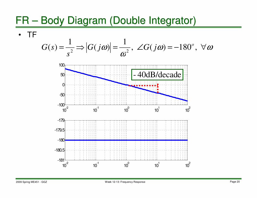
• TF
FR FR –– Body Diagram (Double Integrator)Body Diagram (Double Integrator)
ωωω
ω ∀−=∠=⇒= ,180)( ,1
)(1
)(22
ojGjG
ssG
e40dB/decad-

2009 Spring ME451 - GGZ Page 21Week 12-13: Frequency Response
• TF
10-2
10-1
100
101
102
-50
-40
-30
-20
-10
0
10-2
10-1
100
101
102
-100
-80
-60
-40
-20
0
Corner frequencyCorner frequency
Straight lineStraight line
approximationapproximation
e20dB/decad-
FR FR –– Body Diagram (1Body Diagram (1stst Order System)Order System)
1
1)(
+=
TssG
<<
>>≈
+=
T
T
TjjG
Tjω
ω
ωω
ω1 if
1 if1
1
1)(
145−
90−
1
1)(
+=
ssG
T
1

2009 Spring ME451 - GGZ Page 22Week 12-13: Frequency Response
• TF
10-2
10-1
100
101
102
0
10
20
30
40
50
10-2
10-1
100
101
102
0
20
40
60
80
100
Mirror image of the Mirror image of the
original bode plot original bode plot
with respect to with respect to ωω--
axis.axis.
FR FR –– Body Diagram (Inversed 1Body Diagram (Inversed 1stst Order System)Order System)
1
1
11)(
−
+=+=
TsTssG
e20dB/decad+

2009 Spring ME451 - GGZ Page 23Week 12-13: Frequency Response
• TF
• Resonant freq
• Peak gain
10-1
100
101
-60
-40
-20
0
20
10-1
100
101
-200
-150
-100
-50
0
resonanceresonance
FR FR –– Body Diagram (2Body Diagram (2ndnd Order System)Order System)
22
2
2)(
nn
n
sssG
ωςω
ω
++=
221: ςωω −=nr
1 if
2
1
12
1
2
<<
≈−
ς
ςςς
90−
180−
1.0=ς
1=ς
1=ς
dB/decade40−
2009 Spring ME451 - GGZ Page 24Week 12-13: Frequency Response
1 0-2
1 0-1
1 00
1 01
1 02
-1
-0 .5
0
0 .5
1
1 0-2
1 0-1
1 00
1 01
1 02
-6 0 0 0
-4 0 0 0
-2 0 0 0
0
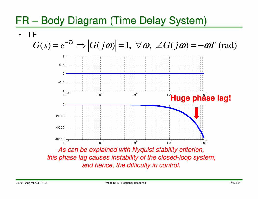
• TF
Huge phase lag!Huge phase lag!
As can be explained with As can be explained with NyquistNyquist stability criterion, stability criterion,
this phase lag causes instability of the closedthis phase lag causes instability of the closed--loop system,loop system,
and hence, the difficulty in control.and hence, the difficulty in control.
FR FR –– Body Diagram (Time Delay System)Body Diagram (Time Delay System)
(rad) )( , ,1)()( TjGjGesG Ts ωωωω −=∠∀=⇒= −

2009 Spring ME451 - GGZ Page 25Week 12-13: Frequency Response
• Use Matlab “bode.m” to obtain precise shape.
• ALWAYS check the correctness of
– Low frequency gain (DC gain)
– High frequency gain
• Example
FR FR –– Body Diagram RemarkBody Diagram Remark
)0(G
)(∞G
dB62)0( ⇒=G
dB2010)( ⇒=∞G
5
)1(10)(
+
+=
s
ssG

2009 Spring ME451 - GGZ Page 26Week 12-13: Frequency Response
• Sketch bode plot.
FR FR –– Body Diagram ExercisesBody Diagram Exercises
110
1)(
+=
ssG
1)( =sG 1.0)( =sG 10)( −=sG
2)( ssG =3)( ssG =
3
1)(
ssG =
110
10)(
+=
ssG 110)( += ssG
12)( += ssG 15
)( +=s
sG42
4)(
2 ++=
sssG

2009 Spring ME451 - GGZ Page 27Week 12-13: Frequency Response
• Bode plot of various simple transfer functions.
– Constant gain
– Differentiator, integrator
– 1st order and 2nd order systems
– Time delay
• Sketching Bode plot is just ….
– to get a rough idea of the characteristic of a system.
– to interpret the result obtained from computer.
– to detect erroneous result from computer.
FR FR –– Body Diagram SummaryBody Diagram Summary

2009 Spring ME451 - GGZ Page 28Week 12-13: Frequency Response
10-2
10-1
100
101
102
19
19.5
20
20.5
21
10-2
10-1
100
101
102
-1
-0.5
0
0.5
1
10-2
10-1
100
101
102
-40
-20
0
20
40
10-2
10-1
100
101
102
89
89.5
90
90.5
91
FR FR –– Body Diagram of Basic Functions Body Diagram of Basic Functions (Review (Review -- 1)1)
KsG =)(
K10
log20
ssG =)(
dB/decade20+

2009 Spring ME451 - GGZ Page 29Week 12-13: Frequency Response
10-2
10-1
100
101
102
-100
-50
0
50
100
10-2
10-1
100
101
102
-181
-180.5
-180
-179.5
-179
10-2
10-1
100
101
102
-40
-20
0
20
40
10-2
10-1
100
101
102
-91
-90.5
-90
-89.5
-89
FR FR –– Body Diagram of Basic Functions Body Diagram of Basic Functions (Review (Review -- 2)2)
ssG
1)( =
2
1)(
ssG =
dB/decade20+dB/decade20−

2009 Spring ME451 - GGZ Page 30Week 12-13: Frequency Response
10-2
10-1
100
101
102
-50
-40
-30
-20
-10
0
10-2
10-1
100
101
102
-100
-80
-60
-40
-20
0
10-2
10-1
100
101
102
0
10
20
30
40
50
10-2
10-1
100
101
102
0
20
40
60
80
100
FR FR –– Body Diagram of Basic Functions Body Diagram of Basic Functions (Review (Review -- 3)3)
1
1)(
+=
TssG
1)( += TssG
dB/decade20+
dB/decade20−
T
1
T
1

2009 Spring ME451 - GGZ Page 31Week 12-13: Frequency Response
10-1
100
101
-60
-40
-20
0
20
10-1
100
101
-200
-150
-100
-50
0
Bode plot of a 2nd order system
FR FR –– Body Diagram of Basic Functions Body Diagram of Basic Functions (Review (Review -- 4)4)
resonanceresonance
22
2
2)(
nn
n
sssG
ωςω
ω
++=
221: ςωω −=nr
1 if
2
1
12
1
2
<<
≈−
ς
ςςς
90−
180−
1.0=ς
1=ς
1=ς
dB/decade40−
Resonant frequency
Peak Gain
2009 Spring ME451 - GGZ Page 32Week 12-13: Frequency Response
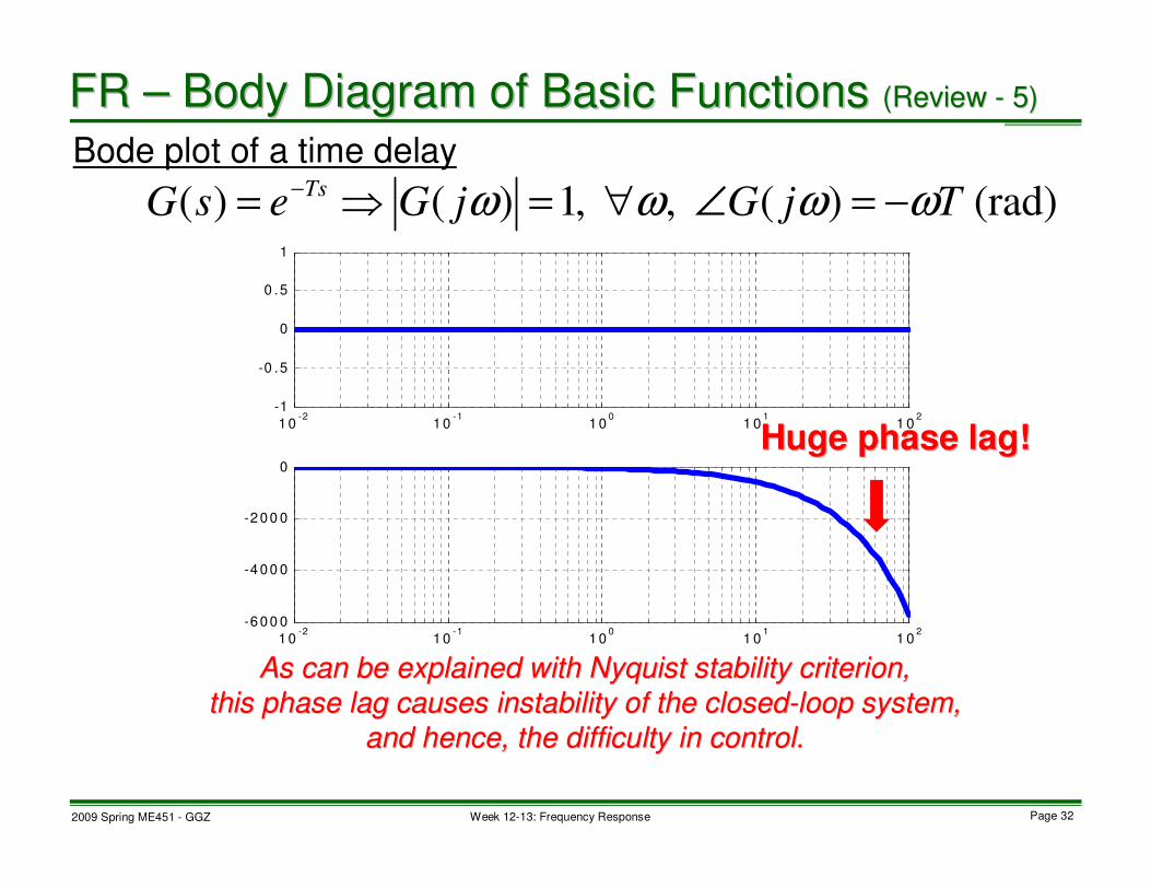
Bode plot of a time delay
FR FR –– Body Diagram of Basic Functions Body Diagram of Basic Functions (Review (Review -- 5)5)
1 0-2
1 0-1
1 00
1 01
1 02
-1
-0 .5
0
0 .5
1
1 0-2
1 0-1
1 00
1 01
1 02
-6 0 0 0
-4 0 0 0
-2 0 0 0
0
Huge phase lag!Huge phase lag!
As can be explained with As can be explained with NyquistNyquist stability criterion, stability criterion,
this phase lag causes instability of the closedthis phase lag causes instability of the closed--loop system,loop system,
and hence, the difficulty in control.and hence, the difficulty in control.
(rad) )( , ,1)()( TjGjGesG Ts ωωωω −=∠∀=⇒= −
2009 Spring ME451 - GGZ Page 33Week 12-13: Frequency Response
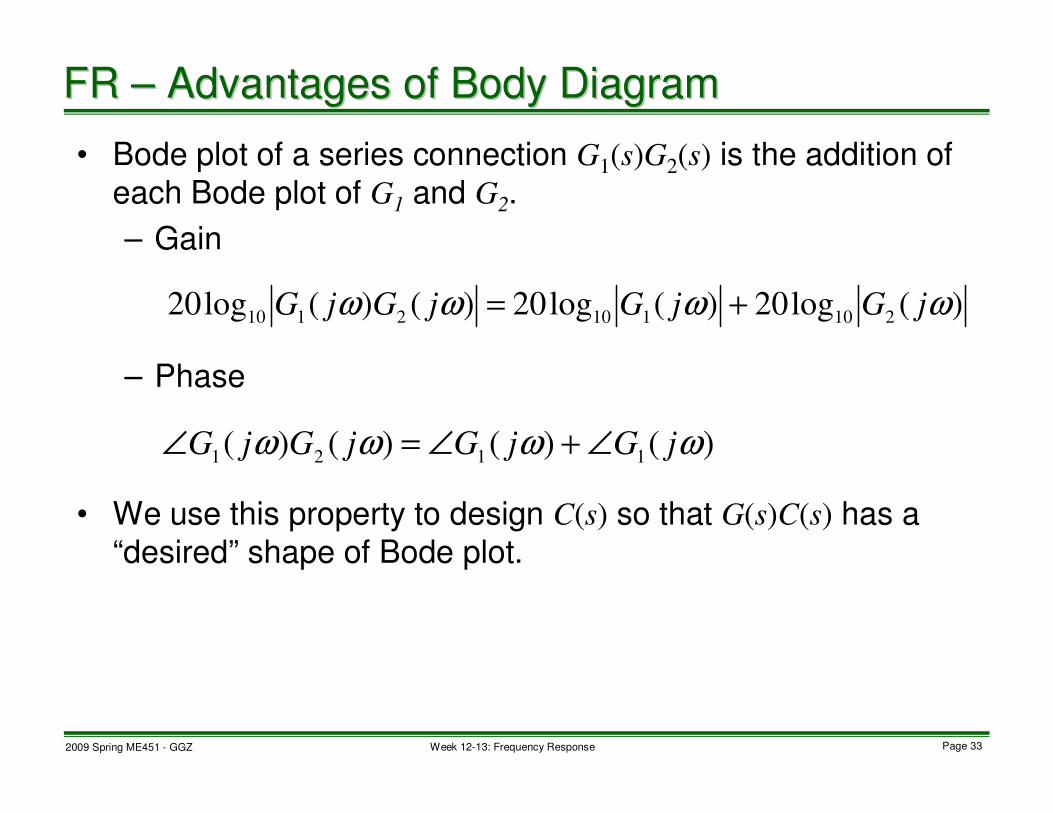
• Bode plot of a series connection G1(s)G2(s) is the addition of
each Bode plot of G1 and G2.
– Gain
– Phase
• We use this property to design C(s) so that G(s)C(s) has a
“desired” shape of Bode plot.
FR FR –– Advantages of Body DiagramAdvantages of Body Diagram
)(log20)(log20)()(log202101102110
ωωωω jGjGjGjG +=
)()()()(1121
ωωωω jGjGjGjG ∠+∠=∠

2009 Spring ME451 - GGZ Page 34Week 12-13: Frequency Response
• Use polar representation
Then,
Therefore,
FR FR –– Short Proofs of Gain and Phase FormulaShort Proofs of Gain and Phase Formula
)()(
212121)()()()(
ωωωωωω jGjjGjejGjGjGjG
∠+∠=
)(log20)(log20
))()((log20)()(log20
210110
21102110
ωω
ωωωω
jGjG
jGjGjGjG
+=
=
)(
222)()(
ωωω jGjejGjG
∠=)(
111)()(
ωωω jGjejGjG
∠=
)()()()(21
)()(
2121 ωωωω ωω
jGjGejGjGjGjjGj
∠+∠=∠=∠∠+∠

2009 Spring ME451 - GGZ Page 35Week 12-13: Frequency Response
• Sketch the Bode plot of a transfer function
1. Decompose G(s) into a product form:
2. Sketch a Bode plot for each component on the same
graph.
3. Add them all on both gain and phase plots.
FR FR –– Example 1 Example 1 (1)(1)
ssG
110)( ⋅=
ssG
10)( =

2009 Spring ME451 - GGZ Page 36Week 12-13: Frequency Response
dBdB
degdeg
--2020
FR FR –– Example 1 Example 1 (2)(2)
ssG
10)( =
ssG
1)(
2=
10)(1 =sG

2009 Spring ME451 - GGZ Page 37Week 12-13: Frequency Response
dBdB
degdeg
--2020
FR FR –– Example 2Example 2
ssG
1)(
2=
1.0)(1 =sG
ssG
1.0)( =

2009 Spring ME451 - GGZ Page 38Week 12-13: Frequency Response
dBdB
degdeg
--2020
--4040ssG
1)(
2=
)12(
1)(
+=
sssG
FR FR –– Example 3Example 3
12
1)(1
+=
ssG
2009 Spring ME451 - GGZ Page 39Week 12-13: Frequency Response
dBdB
degdeg
+20+20
--2020
+45+45 --4545
--4545
FR FR –– Example 4Example 4
)10(
)1(10)(
+
+=
s
ssG
1)(1
+= ssG
11.0
1)(
2+
=s
sG
2009 Spring ME451 - GGZ Page 40Week 12-13: Frequency Response
dBdB
degdeg
+20+20
--4040
+45+45 --4545
--9090
--2020
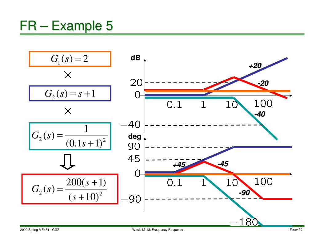
FR FR –– Example 5Example 5
2)(1
=sG
1)(2
+= ssG
22)11.0(
1)(
+=
ssG
22)10(
)1(200)(
+
+=
s
ssG

2009 Spring ME451 - GGZ Page 41Week 12-13: Frequency Response
• Sketch the Bode plot of:
• Find a transfer function having the gain plot:
0dB0dB
20dB20dB
22 2020
--4040+20+20
Ans.Ans.
FR FR –– ExercisesExercises
2)1(
20)(
+=
sssG
2)1(
8)(
+=
s
ssG
2
2)(
s
ssG
+=
)2(
2)(
2 +=
sssG
)1()1(
5)(
212
201 ++
=ss
ssG

2009 Spring ME451 - GGZ Page 42Week 12-13: Frequency Response
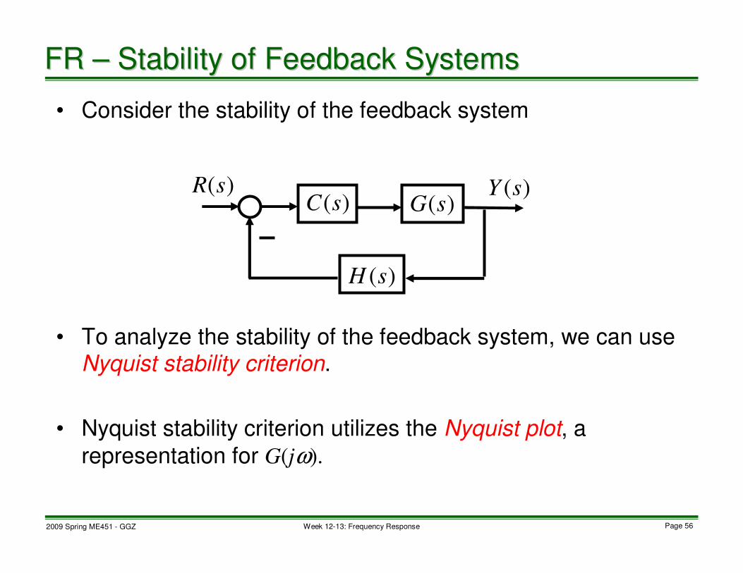
• Consider the feedback system
• Fundamental questions
– If G, C, and H are stable, is closed-loop system always
stable?
– If G, C, and H are unstable, is closed-loop system always
unstable?
FR FR –– Stability of Feedback SystemsStability of Feedback Systems
)(sG)(sC
)(sH
)(sR )(sY

2009 Spring ME451 - GGZ Page 43Week 12-13: Frequency Response
• Closed-loop stability can be determined by the roots of
the characteristic equation
• CL system is stable if the Characteristic Equation has all
roots in the open left half plane.
• How to check the stability?
– Compute all the roots.
– Routh-Hurwitz stability criterion
– Nyquist stability criterion
FR FR –– ClosedClosed--Loop Stability CriterionLoop Stability Criterion
0)(1 =+ sL )()()(:)( sHsCsGsL =

2009 Spring ME451 - GGZ Page 44Week 12-13: Frequency Response
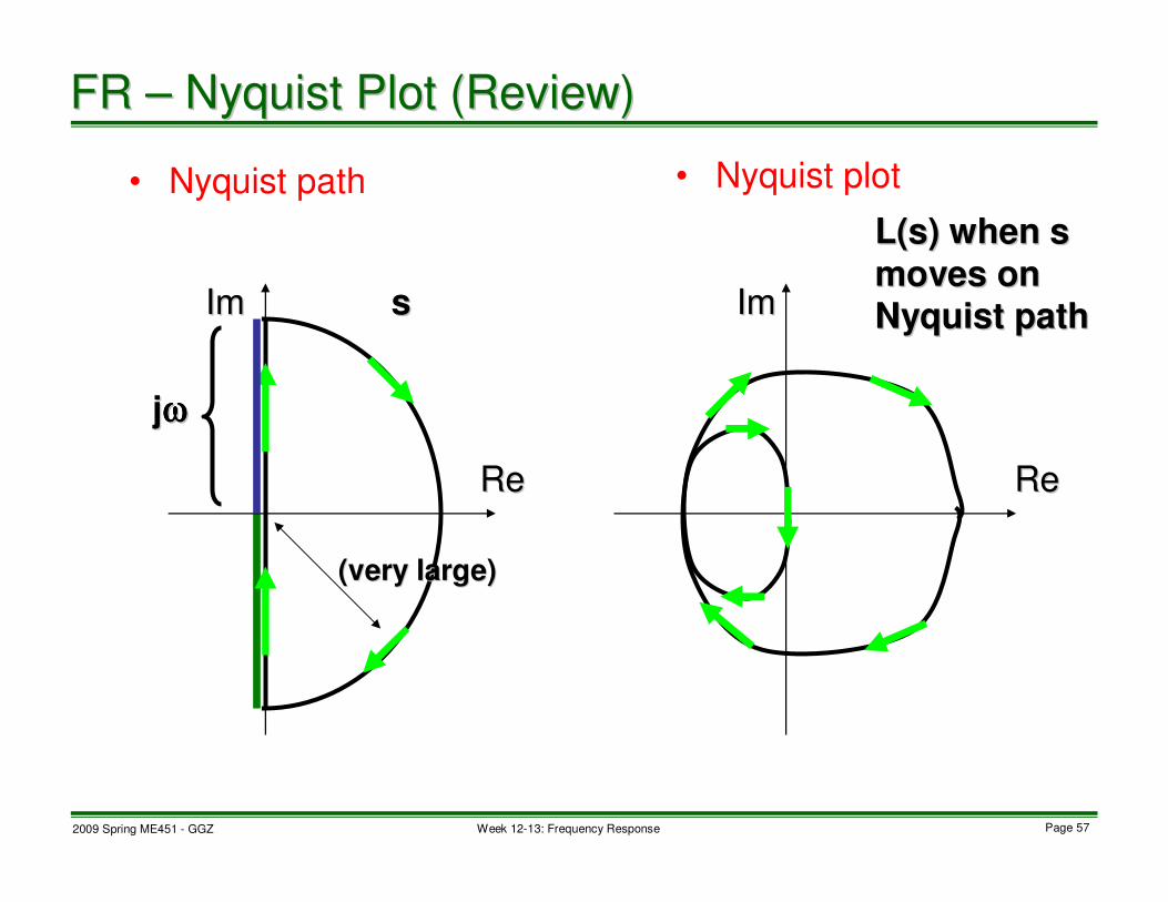
• Nyquist path
(very large)(very large)
• Nyquist plot
ss
L(sL(s) when s ) when s
moves on moves on
NyquistNyquist path path
ReRe
ImIm
ReRe
ImIm
jjωωωωωωωω
FR FR –– NyquistNyquist PlotPlot
2009 Spring ME451 - GGZ Page 45Week 12-13: Frequency Response
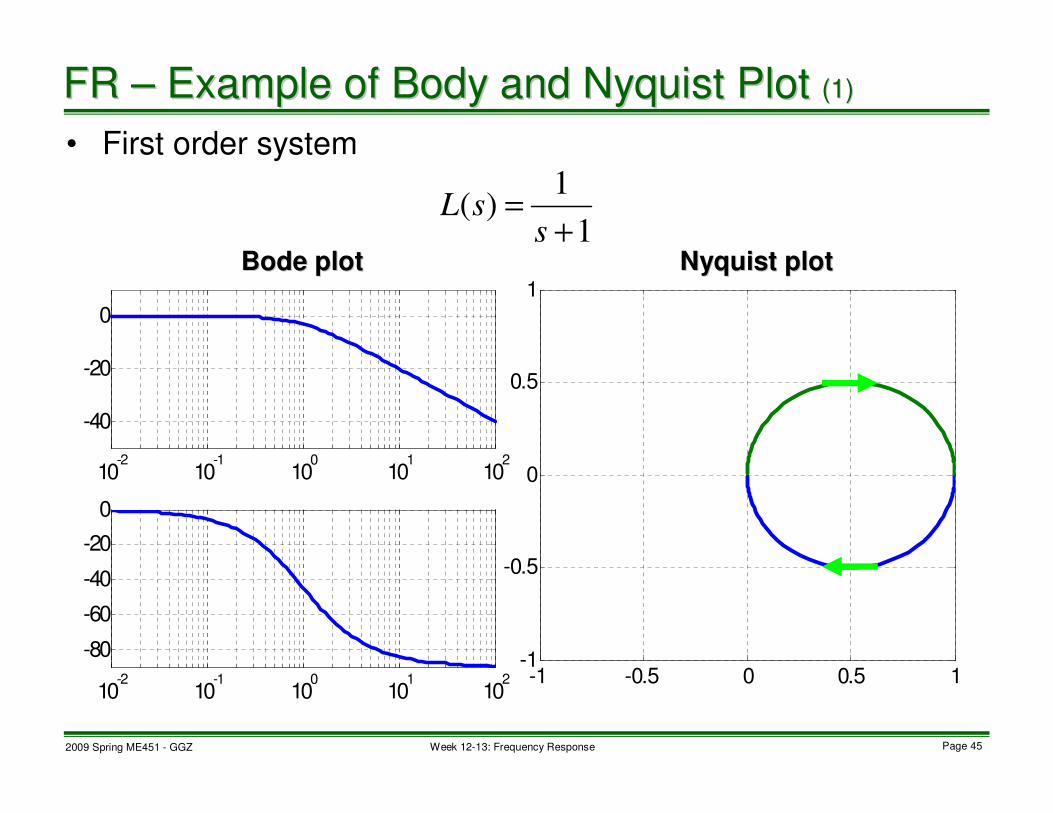
• First order system
10-2
10-1
100
101
102
-40
-20
0
10-2
10-1
100
101
102
-80
-60
-40
-20
0
Bode plotBode plot NyquistNyquist plotplot
-1 -0.5 0 0.5 1-1
-0.5
0
0.5
1
FR FR –– Example of Body and Example of Body and NyquistNyquist Plot Plot (1)(1)
1
1)(
+=
ssL

2009 Spring ME451 - GGZ Page 46Week 12-13: Frequency Response
• Second order system
Bode plotBode plot
10-2
10-1
100
101
102
-100
-50
0
10-2
10-1
100
101
102
-150
-100
-50
0
NyquistNyquist plotplot
-1 -0.5 0 0.5 1-1
-0.5
0
0.5
1
FR FR –– Example of Body and Example of Body and NyquistNyquist Plot Plot (2)(2)
2)1(
1)(
+=
ssL

2009 Spring ME451 - GGZ Page 47Week 12-13: Frequency Response
• Third order system
Bode plotBode plot
10-2
10-1
100
101
102
-150
-100
-50
0
10-2
10-1
100
101
102
-200
-100
0
NyquistNyquist plotplot
-1 -0.5 0 0.5 1-1
-0.5
0
0.5
1
FR FR –– Example of Body and Example of Body and NyquistNyquist Plot Plot (3)(3)
3)1(
1)(
+=
ssL

2009 Spring ME451 - GGZ Page 48Week 12-13: Frequency Response
• Z: # of CL poles in open RHP
• P: # of OL poles in open RHP (given)
• N: # of clockwise encirclement around -1
by Nyquist plot of OL transfer function L(s)
(counted by using Nyquist plot of L(s))
Remark: N = -1: a counter-clockwise encirclement
FR FR –– NyquistNyquist Stability CriterionStability Criterion
0: stable is system CL =+=⇔ NPZ

2009 Spring ME451 - GGZ Page 49Week 12-13: Frequency Response
• Clockwise
ReRe
ImIm
• Counter-clockwise
ReRe
ImIm
FR FR –– Encirclement on Encirclement on NyquistNyquist PlotPlot

2009 Spring ME451 - GGZ Page 50Week 12-13: Frequency Response
• If Nyquist plot passes the point -1, it means that the
closed-loop system has a pole on the imaginary axis
(and thus, not stable).
ReRe
ImIm
FR FR –– Encirclement on Encirclement on NyquistNyquist Plot RemarkPlot Remark
00 somefor 1)( ωω −=jL
00 somefor 0)(1 ωω =+ jL
0at pole a has system CL ωj

2009 Spring ME451 - GGZ Page 51Week 12-13: Frequency Response
-1.5 -1 -0.5 0 0.5 1-1
-0.5
0
0.5
1
-1.5 -1 -0.5 0 0.5 1-1
-0.5
0
0.5
1
For For L(sL(s) of 2) of 2ndnd order and constant numerator, order and constant numerator,
gain increase never lead to unstable CL system!gain increase never lead to unstable CL system!
Gain increaseGain increase
FR FR –– Example for 2Example for 2ndnd Order Order L(sL(s))
2)1(
1)(
+=
ssL
2)1(
10)(
+=
ssL
stable CL0,0 ⇒== NP stable CL0,0 ⇒== NP

2009 Spring ME451 - GGZ Page 52Week 12-13: Frequency Response
-5 0 5 10 15-15
-10
-5
0
5
10
15
-2 -1.5 -1 -0.5 0 0.5 1-1
-0.5
0
0.5
1
Gain increaseGain increase
For For L(sL(s) with relative degree 3, ) with relative degree 3,
gain increase eventually lead to unstable CL system!gain increase eventually lead to unstable CL system!
FR FR –– Example for 3Example for 3rdrd Order Order L(sL(s))
stable CL0,0 ⇒== NP unstable CL1,0 ⇒== NP
3)1(
1)(
+=
ssL
3)1(
15)(
+=
ssL
2009 Spring ME451 - GGZ Page 53Week 12-13: Frequency Response
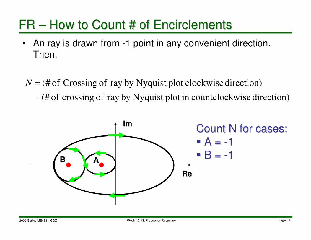
BB
• An ray is drawn from -1 point in any convenient direction. Then,
ReRe
ImIm
AA
Count N for cases:Count N for cases:
�� A = A = --11
�� B = B = --11
FR FR –– How to Count # of EncirclementsHow to Count # of Encirclements
direction) wisecountclockin plot Nyquist by ray of crossing of (# -
direction) clockwiseplot Nyquist by ray of Crossing of #(=N

2009 Spring ME451 - GGZ Page 54Week 12-13: Frequency Response
• Nyquist stability criterion allows us to determine the stability
of CL system from a knowledge of the G(jω) of OL system.
• If an OL system is stable, it requires only frequency
response data of OL system (TF model L(s) is not
necessary).
• It can deal with time delay, which Routh-Hurwitz criterion
cannot.
• We often draw only half of Nyquist plot. (The other half is
mirror image w.r.t. real axis.)
FR FR –– Notes on Notes on NyquistNyquist Stability CriterionStability Criterion

2009 Spring ME451 - GGZ Page 55Week 12-13: Frequency Response
• Nyquist plot (Matlab command: “nyquist.m”)
• Nyquist stability criterion for feedback stability
• Exercises: For (half of) Nyquist plot below, count N for
each case.
•• A = A = --1 1 (Ans. N=2)(Ans. N=2)
•• B = B = --1 1 (Ans. N=0)(Ans. N=0)
•• C = C = --1 1 (Ans. N=2)(Ans. N=2)
•• D = D = --1 1 (Ans. N=0)(Ans. N=0)
•• E = E = --1 1 (Ans. N=2)(Ans. N=2)
•• F = F = --1 1 (Ans. N=0)(Ans. N=0)
AA
BB
CC
DD
EE
FF
FR FR –– NyquistNyquist Summary and Summary and ExcerciseExcercise
2009 Spring ME451 - GGZ Page 56Week 12-13: Frequency Response
• Consider the stability of the feedback system
• To analyze the stability of the feedback system, we can use Nyquist stability criterion.
• Nyquist stability criterion utilizes the Nyquist plot, a
representation for G(jω).
FR FR –– Stability of Feedback SystemsStability of Feedback Systems
)(sG)(sC
)(sH
)(sR )(sY
2009 Spring ME451 - GGZ Page 57Week 12-13: Frequency Response
• Nyquist path
(very large)(very large)
• Nyquist plot
ss
L(sL(s) when s ) when s
moves on moves on
NyquistNyquist path path
ReRe
ImIm
ReRe
ImIm
jjωωωωωωωω
FR FR –– NyquistNyquist Plot (Review)Plot (Review)

2009 Spring ME451 - GGZ Page 58Week 12-13: Frequency Response
• Z: # of CL poles in open RHP
• P: # of OL poles in open RHP (given)
• N: # of clockwise encirclement around -1
by Nyquist plot of OL transfer function L(s)
(counted by using Nyquist plot of L(s))
Remark: N = -1: a counter-clockwise encirclement
FR FR –– NyquistNyquist Stability Criterion (Review)Stability Criterion (Review)
0: stable is system CL =+=⇔ NPZ
2009 Spring ME451 - GGZ Page 59Week 12-13: Frequency Response
• Unstable L(s)
• Stable L(s)
• L(s) with an integrator
• L(s) with a double integrator
• L(s) with a time-delay
FR FR –– NyquistNyquist Stability (More Examples)Stability (More Examples)

2009 Spring ME451 - GGZ Page 60Week 12-13: Frequency Response
-1.2 -1 -0.8 -0.6 -0.4 -0.2 0-0.1
-0.05
0
0.05
0.1
FR FR –– NyquistNyquist Stability Example Stability Example (Unstable (Unstable L(sL(s) (1))) (1))
stable is system CL0)1(1: ⇒=−+=+= NPZ
)3)(2)(1(
8)(
++−=
ssssL

2009 Spring ME451 - GGZ Page 61Week 12-13: Frequency Response
-2 -1.5 -1 -0.5 0
-0.1
-0.05
0
0.05
0.1
0.15
-1 -0.8 -0.6 -0.4 -0.2 0
-0.06
-0.04
-0.02
0
0.02
0.04
0.06Gain increaseGain increase Gain decreaseGain decrease
FR FR –– NyquistNyquist Stability Example Stability Example (Unstable (Unstable L(sL(s) (2))) (2))
)3)(2)(1(
11)(
++−=
ssssL
)3)(2)(1(
5)(
++−=
ssssL
unstable is system CL
2)1(1:
⇒
=++=+= NPZ
unstable is system CL
1)0(1:
⇒
=++=+= NPZ

2009 Spring ME451 - GGZ Page 62Week 12-13: Frequency Response
Interpretation by root locus
11--22--33
ReRe
ImIm
Open loop gain increase will first stabilize, Open loop gain increase will first stabilize,
and then, destabilize the closedand then, destabilize the closed--loop system.loop system.Stabilizing!Stabilizing!
Destabilizing!Destabilizing!
FR FR –– NyquistNyquist Stability Example Stability Example (Unstable (Unstable L(sL(s) (3))) (3))
)3)(2)(1(
1)(
++−=
ssssL

2009 Spring ME451 - GGZ Page 63Week 12-13: Frequency Response
• IF P=0 (i.e., if L(s) has no pole in open RHP or stable)
This fact is very important since openThis fact is very important since open--loop systems loop systems
in many practical problems have no pole in open RHP!in many practical problems have no pole in open RHP!
FR FR –– NyquistNyquist Stability Criterion: A Special CaseStability Criterion: A Special Case
0stable is system CL =+=⇔ NPZ:
0stable is system CL =⇔ N

2009 Spring ME451 - GGZ Page 64Week 12-13: Frequency Response
-1 0 1 2 3-3
-2.5
-2
-1.5
-1
-0.5
0
0.5
-5 0 5 10 15 20-15
-10
-5
0
CL stableCL stable CL unstableCL unstable
FR FR –– NyquistNyquist Stability Example Stability Example (stable (stable L(sL(s) (1))) (1))
)3)(2)(1(
20)(
+++=
ssssL
)3)(2)(1(
100)(
+++=
ssssL

2009 Spring ME451 - GGZ Page 65Week 12-13: Frequency Response
Interpretation by root locus
--11--22--33
ReRe
ImIm
Open loop gain increase will Open loop gain increase will
destabilize the closeddestabilize the closed--loop system.loop system.
FR FR –– NyquistNyquist Stability Example Stability Example (stable (stable L(sL(s) (2))) (2))
)3)(2)(1(
1)(
+++=
ssssL
2009 Spring ME451 - GGZ Page 66Week 12-13: Frequency Response
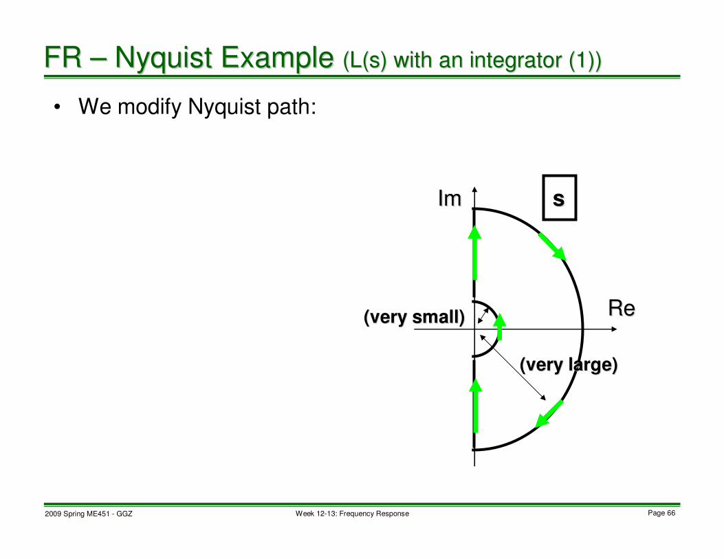
• We modify Nyquist path:
(very large)(very large)
ss
ReRe
ImIm
(very small)(very small)
FR FR –– NyquistNyquist Example Example ((L(sL(s) with an integrator (1))) with an integrator (1))

2009 Spring ME451 - GGZ Page 67Week 12-13: Frequency Response
-1 -0.8 -0.6 -0.4 -0.2 0
-15
-10
-5
0
5
10
15
FR FR –– NyquistNyquist Example Example ((L(sL(s) with an integrator (2))) with an integrator (2))
)1(
1)(
+=
sssL
Stable CL0,0 ⇒== NP
2009 Spring ME451 - GGZ Page 68Week 12-13: Frequency Response
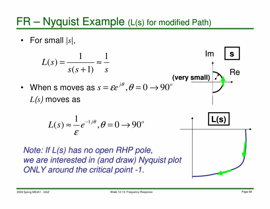
• For small |s|,
• When s moves as
L(s) moves as
ReRe
ImIm
(very small)(very small)
ss
L(sL(s))
Note: If Note: If L(sL(s) has no open RHP pole,) has no open RHP pole,
we are interested in (and draw) we are interested in (and draw) NyquistNyquist plot plot
ONLY around the critical point ONLY around the critical point --1.1.
FR FR –– NyquistNyquist Example Example ((L(sL(s) for modified Path)) for modified Path)
ssssL
1
)1(
1)( ≈
+=
ojes 900, →== θε θ
ojesL 900,
1)( 1 →=≈ − θ
ε
θ

2009 Spring ME451 - GGZ Page 69Week 12-13: Frequency Response
-5 -4 -3 -2 -1 0-5
0
5
FR FR –– NyquistNyquist Example Example ((L(sL(s) with an double integrator)) with an double integrator)
)1(
1)(
2+
=ss
sL
unStable CL2,0 ⇒== NP

2009 Spring ME451 - GGZ Page 70Week 12-13: Frequency Response
-1 0 1 2 3-3
-2.5
-2
-1.5
-1
-0.5
0
0.5
RouthRouth--Hurwitz is NOT applicable!Hurwitz is NOT applicable!
FR FR –– NyquistNyquist Example Example ((L(sL(s) with a time delay (1))) with a time delay (1))
)3)(2)(1(
20)(
+++=
ssssL
unStable CL1,0 ⇒== NP
Stable CL0,0 ⇒== NP
)3)(2)(1(
20)(
7.0
+++=
−
sss
esL
s

2009 Spring ME451 - GGZ Page 71Week 12-13: Frequency Response
1 0-2
1 0-1
1 00
1 01
1 02
-1
-0 .5
0
0 .5
1
1 0-2
1 0-1
1 00
1 01
1 02
-6 0 0 0
-4 0 0 0
-2 0 0 0
0
• TF
Huge phase lag!Huge phase lag!
As can be explained with As can be explained with NyquistNyquist stability criterion, stability criterion,
this phase lag causes instability of the closedthis phase lag causes instability of the closed--loop system,loop system,
and hence, the difficulty in control.and hence, the difficulty in control.
(rad) )( , ,1)()( TjGjGesG Ts ωωωω −=∠∀=⇒= −
FR FR –– NyquistNyquist Example Example ((L(sL(s) with a time delay (2))) with a time delay (2))

2009 Spring ME451 - GGZ Page 72Week 12-13: Frequency Response
• Examples for Nyquist stability criterion
• Next,
– PID control
– Relative stability
• Exercise: Suppose L(s) is stable and has Nyquist plot below. Find the range of OL gain K>0 for which CL
system is stable.
--0.50.5--22--3.33.3
(Ans. 0 < K< 1/3.3, (Ans. 0 < K< 1/3.3, ½½ < K <2)< K <2)
--11
FR FR –– NyquistNyquist SummarySummary