FPGA-Based DOCSIS Upstream

Demodulation

A Thesis Submitted

to the College of Graduate Studies and Research

in Partial Fulfillment of the Requirements

for the Degree of Doctor of Philosophy

in the Department of Electrical and Computer Engineering

University of Saskatchewan

by

Brian Berscheid

Saskatoon, Saskatchewan, Canada

c© Copyright Brian Berscheid, July, 2011. All rights reserved.

Permission to Use

In presenting this thesis in partial fulfillment of the requirements for a Postgraduate

degree from the University of Saskatchewan, it is agreed that the Libraries of this

University may make it freely available for inspection. Permission for copying of this

thesis in any manner, in whole or in part, for scholarly purposes may be granted by

the professors who supervised this thesis work or, in their absence, by the Head of

the Department of Electrical and Computer Engineering or the Dean of the College

of Graduate Studies and Research at the University of Saskatchewan. Any copying,

publication, or use of this thesis, or parts thereof, for financial gain without the

written permission of the author is strictly prohibited. Proper recognition shall be

given to the author and to the University of Saskatchewan in any scholarly use which

may be made of any material in this thesis.

Request for permission to copy or to make any other use of material in this thesis

in whole or in part should be addressed to:

Head of the Department of Electrical and Computer Engineering

57 Campus Drive

University of Saskatchewan

Saskatoon, Saskatchewan, Canada

S7N 5A9

i

Acknowledgments

I would like to express my appreciation to my supervisors, Professor J. Eric Salt

and Professor Ha H. Nguyen for their guidance and teaching throughout my pursuit

of this degree. They have truly taken an interest in my work, and have provided

outstanding support over the years. I feel very fortunate to have had the opportunity

to work with such wonderful supervisors.

I would also like to thank Professors Robert Johanson, Aryan Saadat-Mehr, and

Doug Degenstein for acting as members of my Ph.D. advisory committee. Their

questions and comments have helped to direct my research.

I would like to thank fellow students Eric Pelet and Zohreh Andalibi, with whom

I have enjoyed many thoughtful discussions and collaborations.

Finally, I would like to express my gratitude to my parents, Bruce and Barbara

Berscheid, who have provided tremendous support, encouragement, and inspiration

over the years.

ii

Abstract

In recent years, the state-of-the-art in field programmable gate array (FPGA)

technology has been advancing rapidly. Consequently, the use of FPGAs is being con-

sidered in many applications which have traditionally relied upon application-specific

integrated circuits (ASICs). FPGA-based designs have a number of advantages over

ASIC-based designs, including lower up-front engineering design costs, shorter time-

to-market, and the ability to reconfigure devices in the field. However, ASICs have

a major advantage in terms of computational resources. As a result, expensive high

performance ASIC algorithms must be redesigned to fit the limited resources available

in an FPGA.

Concurrently, coaxial cable television and internet networks have been undergoing

significant upgrades that have largely been driven by a sharp increase in the use

of interactive applications. This has intensified demand for the so-called upstream

channels, which allow customers to transmit data into the network. The format

and protocol of the upstream channels are defined by a set of standards, known as

DOCSIS 3.0, which govern the flow of data through the network.

Critical to DOCSIS 3.0 compliance is the upstream demodulator, which is re-

sponsible for the physical layer reception from all customers. Although upstream

demodulators have typically been implemented as ASICs, the design of an FPGA-

based upstream demodulator is an intriguing possibility, as FPGA-based demodula-

tors could potentially be upgraded in the field to support future DOCSIS standards.

Furthermore, the lower non-recurring engineering costs associated with FPGA-based

designs could provide an opportunity for smaller companies to compete in this market.

The upstream demodulator must contain complicated synchronization circuitry

to detect, measure, and correct for channel distortions. Unfortunately, many of the

synchronization algorithms described in the open literature are not suitable for either

upstream cable channels or FPGA implementation. In this thesis, computationally

inexpensive and robust synchronization algorithms are explored. In particular, algo-

iii

rithms for frequency recovery and equalization are developed.

The many data-aided feedforward frequency offset estimators analyzed in the lit-

erature have not considered intersymbol interference (ISI) caused by micro-reflections

in the channel. It is shown in this thesis that many prominent frequency offset es-

timation algorithms become biased in the presence of ISI. A novel high-performance

frequency offset estimator which is suitable for implementation in an FPGA is de-

rived from first principles. Additionally, a rule is developed for predicting whether

a frequency offset estimator will become biased in the presence of ISI. This rule is

used to establish a channel excitation sequence which ensures the proposed frequency

offset estimator is unbiased.

Adaptive equalizers that compensate for the ISI take a relatively long time to

converge, necessitating a lengthy training sequence. The convergence time is reduced

using a two step technique to seed the equalizer. First, the ISI equivalent model of

the channel is estimated in response to a specific short excitation sequence. Then,

the estimated channel response is inverted with a novel algorithm to initialize the

equalizer. It is shown that the proposed technique, while inexpensive to implement

in an FPGA, can decrease the length of the required equalizer training sequence by

up to 70 symbols.

It is shown that a preamble segment consisting of repeated 11-symbol Barker

sequences which is well-suited to timing recovery can also be used effectively for

frequency recovery and channel estimation. By performing these three functions

sequentially using a single set of preamble symbols, the overall length of the preamble

may be further reduced.

iv

Table of Contents

Permission to Use i

Acknowledgments ii

Abstract iii

Table of Contents v

List of Tables x

List of Figures xi

List of Abbreviations xv

1 Introduction 1

1.1 Motivation . . . . . . . . . . . . . . . . . . . . . . . . . . . . . . . . . 1

1.1.1 The Cable Industry . . . . . . . . . . . . . . . . . . . . . . . . 1

1.1.2 FPGAs . . . . . . . . . . . . . . . . . . . . . . . . . . . . . . 4

1.2 FPGA-Based DOCSIS Upstream Demodulator . . . . . . . . . . . . . 5

1.2.1 Problem Statement . . . . . . . . . . . . . . . . . . . . . . . . 6

1.2.2 Organization of Thesis and Main Contributions . . . . . . . . 8

2 Upstream Channel Operation 10

2.1 Upstream Physical Layer . . . . . . . . . . . . . . . . . . . . . . . . . 10

2.1.1 Basic QAM Theory . . . . . . . . . . . . . . . . . . . . . . . . 10

2.1.2 Channel Impairments . . . . . . . . . . . . . . . . . . . . . . . 18

Additive White Gaussian Noise . . . . . . . . . . . . . . . . . 18

v

Timing Offset . . . . . . . . . . . . . . . . . . . . . . . . . . . 20

Frequency and Phase Offset . . . . . . . . . . . . . . . . . . . 21

Channel Echoes . . . . . . . . . . . . . . . . . . . . . . . . . . 23

2.2 MAC Layer Control . . . . . . . . . . . . . . . . . . . . . . . . . . . . 26

2.2.1 Overview . . . . . . . . . . . . . . . . . . . . . . . . . . . . . 26

2.2.2 Ranging Mode . . . . . . . . . . . . . . . . . . . . . . . . . . . 28

2.2.3 Traffic Mode . . . . . . . . . . . . . . . . . . . . . . . . . . . . 32

3 Demodulator Architecture 34

3.1 High-Level Architecture . . . . . . . . . . . . . . . . . . . . . . . . . 34

3.1.1 Analog Front End . . . . . . . . . . . . . . . . . . . . . . . . . 35

3.1.2 Digital Front End . . . . . . . . . . . . . . . . . . . . . . . . . 37

3.1.3 Symbol Recovery . . . . . . . . . . . . . . . . . . . . . . . . . 38

4 Frequency and Phase Recovery 44

4.1 Introduction . . . . . . . . . . . . . . . . . . . . . . . . . . . . . . . . 44

4.2 Performance Limits . . . . . . . . . . . . . . . . . . . . . . . . . . . . 45

4.3 Maximum Likelihood Estimators . . . . . . . . . . . . . . . . . . . . 48

4.4 Frequency Offset Estimator . . . . . . . . . . . . . . . . . . . . . . . 50

4.4.1 Previous Work . . . . . . . . . . . . . . . . . . . . . . . . . . 50

4.4.2 Derivation from First Principles . . . . . . . . . . . . . . . . . 51

Phase Noise Model . . . . . . . . . . . . . . . . . . . . . . . . 51

The Estimator - Insight and Performance . . . . . . . . . . . . 53

vi

The Effect of ISI . . . . . . . . . . . . . . . . . . . . . . . . . 60

Implementation Details . . . . . . . . . . . . . . . . . . . . . . 62

Simulation Results . . . . . . . . . . . . . . . . . . . . . . . . 65

Frequency Offset Correction . . . . . . . . . . . . . . . . . . . 70

4.5 Phase Estimator . . . . . . . . . . . . . . . . . . . . . . . . . . . . . 72

4.5.1 Maximum Likelihood Estimator . . . . . . . . . . . . . . . . . 73

4.5.2 Estimator Selection . . . . . . . . . . . . . . . . . . . . . . . . 74

4.5.3 Estimator Analysis . . . . . . . . . . . . . . . . . . . . . . . . 75

4.5.4 Simulation Results . . . . . . . . . . . . . . . . . . . . . . . . 76

4.5.5 Phase Offset Correction . . . . . . . . . . . . . . . . . . . . . 79

5 Equalization 81

5.1 Introduction . . . . . . . . . . . . . . . . . . . . . . . . . . . . . . . . 81

5.1.1 Previous Work . . . . . . . . . . . . . . . . . . . . . . . . . . 83

5.1.2 Problem Formulation . . . . . . . . . . . . . . . . . . . . . . . 85

5.2 Estimation of the ISI Equivalent Filter Coefficients . . . . . . . . . . 89

5.2.1 Intuitive Method . . . . . . . . . . . . . . . . . . . . . . . . . 89

5.2.2 Length of ISI Equivalent Filter . . . . . . . . . . . . . . . . . 93

5.2.3 Linear MVU Theory for ISI Equivalent Filter . . . . . . . . . 96

5.2.4 Estimator Selection . . . . . . . . . . . . . . . . . . . . . . . . 98

Perfect Excitation Sequences . . . . . . . . . . . . . . . . . . . 99

Complementary Code-Based Excitation Sequences . . . . . . . 100

vii

Impulse-Like Excitation Sequences . . . . . . . . . . . . . . . 101

Barker-Based Excitation Sequences . . . . . . . . . . . . . . . 106

5.2.5 Effect of Phase Rotation on ISI Estimation . . . . . . . . . . . 110

5.3 Initialization of Equalizer Coefficients . . . . . . . . . . . . . . . . . . 111

5.3.1 Overview of Common Equalization Techniques . . . . . . . . . 111

5.3.2 Post-Main-Path Initialization Technique . . . . . . . . . . . . 113

Proof that Post-Main-Path Filter is Minimum Phase . . . . . 115

Coefficient Computation . . . . . . . . . . . . . . . . . . . . . 118

5.3.3 Incorporating Pre-Main-Path Information for Initialization . . 122

5.3.4 Computational Complexity . . . . . . . . . . . . . . . . . . . . 124

5.4 Simulation Results . . . . . . . . . . . . . . . . . . . . . . . . . . . . 126

5.4.1 Impulse-Like ISI Estimator . . . . . . . . . . . . . . . . . . . . 126

5.4.2 Barker-Based ISI Estimators . . . . . . . . . . . . . . . . . . . 131

6 Contributions and Conclusions 135

6.1 Frequency Recovery Contributions . . . . . . . . . . . . . . . . . . . . 135

6.2 Equalization Contributions . . . . . . . . . . . . . . . . . . . . . . . . 137

6.3 Conclusions . . . . . . . . . . . . . . . . . . . . . . . . . . . . . . . . 139

A Maximum Likelihood Frequency and Phase Offset Estimation 141

B Detailed Discussion of ISI Estimation Schemes 144

B.1 4-Symbol Perfect Sequence . . . . . . . . . . . . . . . . . . . . . . . . 144

B.2 5-Symbol Impulse-Like Sequence . . . . . . . . . . . . . . . . . . . . . 145

viii

B.3 5-Symbol Barker-Based Sequence . . . . . . . . . . . . . . . . . . . . 148

B.4 11-Symbol Barker-Based Sequence . . . . . . . . . . . . . . . . . . . . 151

B.5 Summary . . . . . . . . . . . . . . . . . . . . . . . . . . . . . . . . . 155

C Reciprocal of a Random Variable 156

D Raising a Random Variable to a Power 157

E Proof of Independence of Noise Samples at Output of ISI Equivalent

Filter 158

ix

List of Tables

1.1 A listing of versions of the DOCSIS standard and their release dates. 2

2.1 Echo channel model. . . . . . . . . . . . . . . . . . . . . . . . . . . . 25

4.1 First channel model for ISI simulation. . . . . . . . . . . . . . . . . . 67

4.2 Second channel model for ISI simulation. . . . . . . . . . . . . . . . . 69

5.1 Channel model for simulation to determine length of ISI equivalent filter. 94

5.2 Performance and complexity of MVU estimators of ISI equivalent co-

efficients. . . . . . . . . . . . . . . . . . . . . . . . . . . . . . . . . . . 109

5.3 Computational complexity of equalization algorithms. . . . . . . . . . 125

5.4 Computational complexity of equalization seeding techniques. . . . . 134

B.1 Performance and complexity of MVU estimators of ISI equivalent co-

efficients. . . . . . . . . . . . . . . . . . . . . . . . . . . . . . . . . . . 155

x

List of Figures

1.1 A typical frequency partitioning of signals in DOCSIS networks. . . . 2

1.2 A high-level overview of the devices in a DOCSIS network. . . . . . . 3

1.3 A high-level block diagram of a digital demodulator. . . . . . . . . . . 7

2.1 Block diagram of a basic QAM modulator. . . . . . . . . . . . . . . . 11

2.2 Constellation diagram for 16-QAM modulation. . . . . . . . . . . . . 12

2.3 Block diagram of a basic QAM demodulator. . . . . . . . . . . . . . . 14

2.4 Graphical representation of a filter meeting the Nyquist criterion. . . 16

2.5 Graphical representation of a filter failing the Nyquist criterion. . . . 17

2.6 Model of AWGN channel. . . . . . . . . . . . . . . . . . . . . . . . . 18

2.7 Eye diagram for QPSK system with α = .1. . . . . . . . . . . . . . . 21

2.8 Received constellation points for 1000 QPSK symbols with ∆f = 10−4

and φo = π/8. . . . . . . . . . . . . . . . . . . . . . . . . . . . . . . . 23

2.9 Linear filter channel model used to represent effect of echoes. . . . . . 24

2.10 Effect of an echo on received baseband signal. . . . . . . . . . . . . . 25

2.11 ISI seen in QPSK constellation due to echo. . . . . . . . . . . . . . . 26

2.12 An example of upstream bandwidth allocation using minislots. . . . . 28

2.13 A spatial distribution of CMs can result in a large variation in message

transit times. . . . . . . . . . . . . . . . . . . . . . . . . . . . . . . . 29

2.14 Ranging minislots provide a buffer to allow for CM timebase variability. 30

2.15 Structure of pre-equalizer in DOCSIS upstream transmitter. . . . . . 31

xi

3.1 High level structure of upstream demodulator. . . . . . . . . . . . . . 34

3.2 Block diagram of complete band sampling analog front end. . . . . . 35

3.3 Block diagram of band-selective sampling analog front end. . . . . . . 36

3.4 Block diagram of digital front end for upstream demodulator. . . . . 37

3.5 Typical structure of a feedback synchronizer. . . . . . . . . . . . . . . 39

3.6 Typical structure of a feedforward synchronizer. . . . . . . . . . . . . 40

3.7 High level block diagram of symbol recovery module. . . . . . . . . . 41

3.8 The structure of an upstream packet. . . . . . . . . . . . . . . . . . . 41

4.1 Modeling AWGN as phase noise. . . . . . . . . . . . . . . . . . . . . 52

4.2 The set of independent estimators which are combined in the decreasing

average-length technique. . . . . . . . . . . . . . . . . . . . . . . . . . 55

4.3 The set of independent estimators which are combined in the equal

average-length technique. . . . . . . . . . . . . . . . . . . . . . . . . . 59

4.4 Modeling the channel ISI as a symbol-rate linear filter. . . . . . . . . 61

4.5 Block diagram of proposed frequency offset estimator. . . . . . . . . . 65

4.6 Variance of proposed frequency offset estimator. . . . . . . . . . . . . 66

4.7 Means of proposed estimator and three well-known estimators in first

ISI channel. . . . . . . . . . . . . . . . . . . . . . . . . . . . . . . . . 67

4.8 Mean squared errors of proposed estimator and three well-known esti-

mators in first ISI channel. . . . . . . . . . . . . . . . . . . . . . . . . 68

4.9 Magnitude responses of simulated ISI channels. . . . . . . . . . . . . 69

4.10 Means of proposed estimator and three well-known estimators in sec-

ond ISI channel. . . . . . . . . . . . . . . . . . . . . . . . . . . . . . . 70

xii

4.11 Mean squared errors of proposed estimator and three well-known esti-

mators in second ISI channel. . . . . . . . . . . . . . . . . . . . . . . 71

4.12 Block diagrm of circuit used to correct for frequency offset. . . . . . . 71

4.13 Hardware implementation of the maximum likelihood phase offset es-

timator. . . . . . . . . . . . . . . . . . . . . . . . . . . . . . . . . . . 74

4.14 Variance of proposed phase estimation algorithm with no residual fre-

quency offset and no channel ISI. . . . . . . . . . . . . . . . . . . . . 77

4.15 Variance of proposed phase estimation algorithm with typical residual

frequency offset and no channel ISI. . . . . . . . . . . . . . . . . . . . 78

4.16 Block diagrm of circuit used to correct for phase offset. . . . . . . . . 80

5.1 Model of the end-to-end system. . . . . . . . . . . . . . . . . . . . . . 85

5.2 ISI model and adaptive equalizer. . . . . . . . . . . . . . . . . . . . . 86

5.3 An abstract view of the idea behind the proposed equalizer seeding

technique. . . . . . . . . . . . . . . . . . . . . . . . . . . . . . . . . . 88

5.4 Energy distribution in coefficients of ISI equivalent filter. . . . . . . . 95

5.5 Average variance of MVU estimator for best possible excitation se-

quences of various lengths. . . . . . . . . . . . . . . . . . . . . . . . . 104

5.6 Autocorrelation function of Barker sequence and Impluse-Like sequence.106

5.7 Parallel representation of the ISI equivalent filter. . . . . . . . . . . . 114

5.8 Summed Magnitude of downsampled raised cosine impulse response. . 117

5.9 Energy distribution in the equalizer taps. . . . . . . . . . . . . . . . . 121

5.10 Circuit for generating estimates of 4 of the most influential coefficients

of the equalizer. . . . . . . . . . . . . . . . . . . . . . . . . . . . . . . 122

xiii

5.11 Structure of cascaded equalizers used to incorporate pre main-path

information. . . . . . . . . . . . . . . . . . . . . . . . . . . . . . . . . 123

5.12 Circuit for equalizer utilizing pre main-path information. . . . . . . . 125

5.13 High-level overview of simulation for MER measurement. . . . . . . . 128

5.14 Tradeoff between step size and MER after 160 updates using the LMS

algorithm. . . . . . . . . . . . . . . . . . . . . . . . . . . . . . . . . . 129

5.15 Equalizer convergence rates using IL sequence for ISI estimation, ∆ =

1/64, threshold = 22dB. . . . . . . . . . . . . . . . . . . . . . . . . . 130

5.16 Equalizer convergence rates using IL sequence for ISI estimation, ∆ =

1/64, threshold = 19dB. . . . . . . . . . . . . . . . . . . . . . . . . . 131

5.17 Comparison of equalizer convergence rates using IL, BB11, and BB11x3

for ISI estimation, ∆ = 1/64, threshold = 22dB. . . . . . . . . . . . . 132

5.18 Comparison of equalizer convergence rates using IL, BB11, and BB11x3

for ISI estimation, ∆ = 1/64, threshold = 22dB. . . . . . . . . . . . . 133

B.1 Matched filter implementation of MVU estimator for perfect 4-symbol

sequence. . . . . . . . . . . . . . . . . . . . . . . . . . . . . . . . . . 146

B.2 MVU estimators for ISI equivalent coefficients using Impulse-Like se-

quence. . . . . . . . . . . . . . . . . . . . . . . . . . . . . . . . . . . . 148

B.3 MVU estimators for ISI equivalent coefficients using 5-symbol Barker-

Based sequence. . . . . . . . . . . . . . . . . . . . . . . . . . . . . . . 151

B.4 MVU estimator for ISI coefficient b−1 using 11-symbol Barker-Based

sequence. . . . . . . . . . . . . . . . . . . . . . . . . . . . . . . . . . 154

B.5 MVU estimator for ISI coefficient b0 using 11-symbol Barker-Based

sequence. . . . . . . . . . . . . . . . . . . . . . . . . . . . . . . . . . 155

xiv

List of Abbreviations

ADC Analog to Digital Converter

AGC Automatic Gain Control

ASIC Application Specific Integrated Circuit

AWGN Additive White Gaussian Noise

BB Barker-Based

BPSK Binary Phase Shift Keying

BSS Band Selective Sampling

CAZAC Constant Amplitude Zero Autocorrelation

CBS Complete Band Sampling

CC Complementary Code

CM Cable Modem

CMTS Cable Modem Termination System

CORDIC COordinate Rotation DIgitial Computer

CRB Cramer-Rao Bound

DSP Digital Signal Processing

DOCSIS Data Over Cable Service Interface Specification

FIR Finite Impulse Response

FPGA Field Programmable Gate Array

IF Intermediate Frequency

IL Impulse-Like

ISI InterSymbol Interference

LMS Least Mean Squares

LUT Look Up Table

MAC Media Access Control

MER Modulation Error Ratio

xv

ML Maximum Likelihood

MSE Mean Squared Error

MSO Multiple System Operator

MVU Minimum Variance Unbiased

NCO Numerically Controlled Oscillator

PD Peak Distortion

PM Post-Main

PPM Pre-and-Post-Main

QAM Quadrature Amplitude Modulation

QPSK Quadrature Phase Shift Keying

RAM Random Access Memory

RF Radio Frequency

RLS Recursive Least Squares

RMS Root Mean Square

RV Random Variable

S-CDMA Synchronous Code Division Multiple Access

SNR Signal to Noise Ratio

SRRC Square Root Raised Cosine

TDMA Time Division Multiple Access

ZF Zero Forcing

xvi

1. Introduction

1.1 Motivation

1.1.1 The Cable Industry

In recent years, cable television providers around the world have been extending

the use of their networks in order to provide telephone and internet services to cus-

tomers in addition to cable television. Such cable companies are commonly referred to

as multiple system operators (MSOs). At the same time, many telephone companies

have diversified into the digital television and internet businesses, placing the MSOs

and telephone companies in direct competition.

The original cable networks were constructed in the United States, beginning in

the late 1940s [1]. Originally, these were exclusively one-way networks, used to dis-

tribute analog television signals from a central cable office (headend) to a multitude

of users. Under this traditional broadcast model, the flow of information was unidi-

rectional; the end users had no need to transmit data back to the headend.

However, in the present day, users of the cable network demand ever higher net-

work speeds in order to take advantage of a variety of bandwidth-intensive applica-

tions such as video-on-demand, online gaming, and videoconferencing. By nature,

interactive applications such as these require each user to transmit data through-

out the network, necessitating a network capable of supporting two-way traffic. The

widespread usage of these types of interactive applications, coupled with the competi-

tion provided by the telephone companies, is driving many cable MSOs to significantly

upgrade the capabilities of their networks.

1

Figure 1.1 A typical frequency partitioning of signals in DOCSIS networks.

Modern cable networks are structured so as to permit simultaneous communica-

tion in two directions: from the headend to the end users (the downstream, or forward

path) and from the end users back to the headend (the upstream, or return path).

To support this full-duplex communication scheme, the frequency spectrum on the

cable is partitioned into two distinct regions. Upstream transmissions are allocated

to the lower frequency region (typically 5-85MHz), while downstream transmissions

are allocated to the higher frequency band (100MHz - 1GHz) [2], as illustrated in

Figure 1.1.

The bidirectional communication system mentioned above is governed by the Data

Over Cable Service Interface Specification (DOCSIS). The DOCSIS standard, which

is issued by a non-partisan organization known as CableLabs, aims to promote in-

teroperability among the various data over cable networks. The original version of

the DOCSIS standard was released in 1997 [3]. Since 1997, data throughput require-

ments for the cable network have continued to increase rapidly. To keep up with this

demand, a number of upgraded versions of the DOCSIS standard have been released,

as highlighted in Table 1.1. The most recent version of the DOCSIS standard is

DOCSIS 3.0, officially released in August 2006 [2].

Table 1.1 A listing of versions of the DOCSIS standard and their release dates.

DOCSIS Version Release Date

1.0 1997

1.1 2001

2.0 2002

3.0 2006

2

cablemodem

dupl

exer

upstream

demodulator

modulatorCMTS

inte

rnet

streamdown

Cable Operator Location

cableplant

Figure 1.2 A high-level overview of the devices in a DOCSIS network.

Throughout the evolution of the DOCSIS standard over the years since the re-

lease of DOCSIS 1.0, there have been numerous changes to both the upstream and

downstream transmission formats. However, by far the greater of the changes have

been to the upstream transmission scheme, reflecting the huge increase in demand

for upstream bandwidth. In order to provide appropriate levels of throughput and

performance for various upstream applications, the DOCSIS standard is extremely

flexible. A large number of parameters for upstream transmission are dynamically

specified and can be modified for each upstream packet transmission. These parame-

ters include: symbol rate, constellation type, payload size, multiple access technique,

and level of error control coding, to name just a few.

As seen in Figure 1.2, there are two main types of devices which communicate over

a DOCSIS network. The device communicating from the headend side of the network

is known as the Cable Modem Termination System (CMTS). At the other end of

the network are a large number of user terminals known as Cable Modems (CM).

The CMTS is essentially the mastermind of the network, responsible for setting the

upstream transmission parameters for every CM in the system, as well as allocating,

monitoring, and coordinating all of the network traffic in both directions. This task

is particularly onerous in the upstream direction, given that the demodulator in the

CMTS must be capable of properly receiving signals from a large number of CMs,

many of which may be transmitting over severely non-ideal channels [4].

In order to take advantage of the higher speeds and new features allowed by

DOCSIS 3.0, the existing CMTSs and CMs in the networks must be replaced with

3

newer DOCSIS 3.0-compliant models. To date, DOCSIS 3.0 has been deployed in a

relatively small number of communities across North America. Thus, the development

and sale of DOCSIS 3.0-compliant CMTSs and CMs may present a significant business

opportunity for cable equipment vendors.

1.1.2 FPGAs

To date, upstream demodulators used in commercially-deployed CMTS systems

have typically been implemented with application-specific integrated circuits (ASICs).

While ASICs tend to provide a very high level of performance, they do suffer from a

number of downsides.

• High non-recurring engineering design costs: In order to manufacture an ASIC,

an extremely expensive set of masks must first be produced for the use during

the lithographic fabrication process [5]. The high cost of this initial fabrica-

tion means that ASICs are not generally commercially viable for lower volume

applications.

• Fixed design: Once an ASIC has been designed and fabricated, its structure

or function may not be changed. Even the smallest functionality change will

require the production of a completely new set of lithographic masks.

• Time to market: Due to the high complexity of the design and fabrication of

ASICs, ASIC designs generally take a relatively long time to complete. This

time to market is further lengthened by the fact that ASIC designs must un-

dergo an arduous testing process prior to fabrication. Since ASICs may not be

modified in any way after fabrication, each ASIC design must be painstakingly

tested prior to the final tape out.

To get around these weaknesses, some cable equipment vendors are considering

field programmable gate arrays (FPGAs) as an alternative to ASICs for the implemen-

tation of an upstream DOCSIS demodulator. FPGAs are integrated circuits whose

4

internal structure may be modified after fabrication through a simple programming

process. This ability to reconfigure the functionality of the device in the field serves

to reduce both design times and time to market, thereby providing advantages over

the traditional ASIC-based approach.

An FPGA contains a finite number of discrete logic components which may be con-

nected together in various ways in order to produce arbitrary behavior. The amount

of logic components contained in a single FPGA has increased dramatically over the

past few years. As a result, FPGAs now have the logic capacity to fulfill the needs of

many complex applications that could previously only be achieved through the use of

ASICs. Consequently, worldwide usage of FPGAs has been steadily increasing since

the introduction of the first commercial FPGA by Xilinx in 1985 [6]. By far the two

largest FPGA manufacturers are Xilinx and Altera.

In addition to generic look-up tables and flip flops, modern FPGAs offer a number

of specialized blocks tailored to specific applications. For example, digital signal pro-

cessing (DSP) blocks allow for high-speed multiplication and accumulation of digital

inputs. Dedicated random access memory (RAM) inside the FPGA allows for easy

storage and retrieval of data. Some FPGAs even provide such features as high-speed

serial transceivers and built-in PowerPC processors.

1.2 FPGA-Based DOCSIS Upstream Demodulator

The high-level goal of this research is to work towards establishing the feasibility

of implementing a DOCSIS 3.0 upstream demodulator in an FPGA. An investigation

into FPGA-based DOCSIS 3.0 upstream demodulators is desirable for a number of

reasons:

• The lower development cost of an FPGA-based solution as compared to an

ASIC-based solution could lower barriers to entry into the CMTS market, pro-

viding smaller companies with a chance to compete.

• The field-reconfigurability of FPGAs is extremely valuable in a frequently-

5

changing environment such as the cable industry. For example, should a new

version of the DOCSIS standard be released in a few years, FPGA-based CMTS

systems could potentially be reconfigured to conform to the new standard

through a firmware upgrade. On the other hand, systems which rely on ASICs

would need to be completely replaced.

• Despite the recent increases in FPGA capacity, FPGAs are typically limited in

terms of the available logic resources when compared to ASICs [7], especially

in terms of dedicated multiplier circuits. Many well-known receiver algorithms

require a large number of multiplications. Consequently, these algorithms are

often not optimal for use in an FPGA and new algorithms which conserve

multipliers may be required. For this reason, the design and implementation of

communications circuits in FPGAs is an intellectually stimulating task.

1.2.1 Problem Statement

As will be discussed in detail in Section 2.1.2, upstream packets in a cable network

are typically corrupted by a number of transmitter-specific impairments. These may

include timing error, carrier frequency and phase error, and channel micro-reflections

(echoes) [8]. In order for a demodulator to provide adequate performance, it is nec-

essary to estimate and correct for these impairments on a packet-by-packet basis.

Digital demodulators are generally structured in a manner similar to that of Fig-

ure 1.3. Note that this high-level structure is not particularly unique; many examples

of similar structures can be found in the open literature [9]. As shown in the fig-

ure, the demodulator contains a number of synchronization blocks which attempt to

compensate for the impairments present in the input signal. In general, the perfor-

mance and cost of a digital demodulator significantly depends upon the quality of

these synchronization blocks [10]. As a consequence, the design of high-performance,

low complexity digital synchronization techniques has been an active research topic

in recent years [11], [12], [13], [14].

The research discussed in this thesis was centered around the design of synchro-

6

Figure 1.3 A high-level block diagram of a digital demodulator.

nization algorithms for DOCSIS upstream channels which are suitable for FPGA-

based implementation. Specifically, the aim of the research was to solve two key

synchronization problems which are prerequisites for an implementation of a DOC-

SIS upstream demodulator:

• Frequency recovery: Many frequency estimation algorithms have been presented

in the literature over the past half century, including [15], [16], [17], [18]. These

references are discussed in detail in Chapter 4. However, the suitability of these

algorithms for the DOCSIS upstream is questionable, as they were not specif-

ically designed to operate in channels with significant intersymbol interference

(ISI). This research aimed to develop a new frequency offset estimator which

is economical to implement in an FPGA and is capable of operating reliably in

the presence of DOCSIS channel echoes.

• Equalization: In order to compensate for the ISI caused by echoes in the ca-

ble plant, an equalizer is required in a DOCSIS upstream demodulator. This

equalizer initially needs to be trained, which is typically a time-consuming and

computationally expensive task, as discussed in [19], [20], [21], which are general

primers on equalization theory. In order to maximize the data throughput of

7

the channel, it is desirable for this training process to be as short as possible.

The goal of this research is to develop a fast-converging equalization scheme for

DOCSIS channels which can be inexpensively implemented in an FPGA.

1.2.2 Organization of Thesis and Main Contributions

The remainder of the thesis is organized as follows. Background material which

is intended to improve the comprehensibility of the thesis as a whole is contained in

Chapters 2 and 3. More specifically, Chapter 2 provides an in-depth look at the oper-

ation and modeling of DOCSIS upstream channels. Next, the proposed demodulator

architecture is outlined in Chapter 3.

Frequency recovery for DOCSIS upstream channels is discussed in Chapter 4.

This chapter contains two main contributions. The first is a novel high-performance

frequency recovery algorithm which has been derived from first principles. The struc-

ture of this algorithm is well-suited to a cost-effective FPGA-based implementation.

The second main contribution of this chapter is a rule which may be used to predict

whether a given frequency offset estimator will be unbiased in the presence of ISI. For

applications where unbiased estimation is required, this rule places a restriction on

the structure of a frequency offset estimator and the preamble sequence upon which

it operates. It is shown that the proposed frequency offset estimator can be made

unbiased for a wide range of preamble sequences.

Chapter 5 then addresses the problem of DOCSIS upstream equalization. The

main contribution of this chapter is a method for reducing the convergence time of

an adaptive equalizer for DOCSIS upstream channels. The method is comprised

of two parts. First, the ISI caused by micro-reflections in the upstream channel is

modeled as an equivalent filter. By observing the distortion caused by the channel

to a known excitation sequence, the equivalent filter’s impulse response is estimated.

Next, the impulse response is crudely inverted in order to initialize the coefficients of

the adaptive equalizer. It is shown that this technique can decrease the length of the

required training sequence for the adaptive equalizer by up to 70 symbols.

8

Finally, Chapter 6, which concludes the thesis, presents a detailed summary of

the research contributions.

9

2. Upstream Channel Operation

2.1 Upstream Physical Layer

The design of a DOCSIS upstream receiver is complicated by the many impair-

ments present in typical upstream signals. In order to understand the synchronization

algorithms which are discussed in this thesis, it is first necessary to understand these

impairments and the effect which they have upon the signal presented to the upstream

demodulator. Accordingly, this section presents background material related to the

physical layer of DOCSIS upstream channels.

2.1.1 Basic QAM Theory

As specified in the DOCSIS standard, data is transferred across upstream cable

channels using Quadrature Amplitude Modulation (QAM). QAM is a well-known

communication technique whereby the magnitudes of two sinusoidal carriers may

be varied independently to convey information. The carriers are chosen to be π/2

radians out of phase, which guarantees orthogonality and prevents the carriers from

interfering with each other. Figure 2.1 illustrates the complete structure of a QAM

modulator/transmitter.

In a QAM modulator, incoming binary data bits are encoded into symbols in a

fashion known to both transmitter and receiver. Such an encoding rule maps a finite

integer k binary digits into one of 2k symbols in a manner prescribed by the standard.

The rate at which the symbol encoder accepts blocks of k binary digits and converts

them into symbols is referred to as the symbol rate. For a digital QAM system,

each symbol is a 2-tuple (aI , aQ), where each of the components is used to amplitude

10

Figure 2.1 Block diagram of a basic QAM modulator.

modulate one of the quadrature carriers. By plotting all of the 2k possible symbols

specified by the encoding rule on a 2-dimensional plane, a visual representation -

typically called a constellation diagram - of the encoding rule may be obtained. An

example constellation diagram for a 16-QAM encoding rule is shown in Figure 2.2.

For each symbol generated by the symbol mapper, two pulses are generated with

weights specified by the values of aI and aQ. Since bandwidth is a precious resource in

modern communication systems, the resulting sequences of pulses are passed through

a low pass pulse shaping filter in order to limit the bandwidth consumed by the

transmission. The filtered signals may be written as the summation of a number of

scaled and delayed versions of the filter’s impulse response as follows:

wI(t) =

∞∑

k=−∞

aIkht(t− kT ) (2.1)

wQ(t) =∞∑

k=−∞

aQkht(t− kT ) (2.2)

where the impulse response of the pulse shaping filter is ht(t) and the symbol period

is T, which has units of seconds per symbol.

11

−3 −2 −1 0 1 2 3

−3

−2

−1

0

1

2

3

Imag

inar

y C

ompo

nent

, aQ

Real Component, aI

Figure 2.2 Constellation diagram for 16-QAM modulation.

At this point, a brief digression is advisable in order to clarify one key matter.

The term ‘symbol’ is a frequent source of confusion when digital communication

systems are discussed. Some sources define a symbol as the baseband continuous-

time waveform which is generated by filtering each output pulse from the symbol

mapper. Others use the term ‘symbol’ to mean a 2-tuple or a complex number.

In this document, the term symbol refers to a complex number which represents

the magnitudes of the pulses from the symbol mapper, i.e. aI + jaQ. For an M-

QAM system, the symbol mapper’s encoding rule defines M possible symbols, each of

which is represented by a complex number. For example, a 4-QAM quadrature phase

shift keying (QPSK) system defines the following four symbols: Esejπ/4, Ese

j3π/4,

Ese−j3π/4, and Ese

−jπ/4, where Es is a constant which represents the average symbol

energy.

Returning to the modulator description, the outputs of the pulse shaping filter are

used to modulate the aforementioned pair of sinusoidal carriers. The two modulated

12

carriers are then added together. The result is a radio frequency (RF) signal which is

suitable for transmission across the cable channel. The transmitted RF signal, x(t),

may be represented mathematically as follows:

x(t) = wI(t)cos(2πfct) + wQ(t)sin(2πfct) (2.3)

It is mathematically convenient to express the baseband signal using complex num-

bers: xb(t) = wI(t) − jwQ(t). Then, equation (2.3) may be written in terms of the

complex baseband signal multiplied by a complex exponential carrier as follows:

x(t) = ℜ[xb(t) · e2πfct]

= ℜ[(wI(t)− jwQ(t)) · e2πfct] (2.4)

The structure of a circuit which demodulates the QAM transmission and recovers

the original binary data is shown in Figure 2.3. For now, it shall be assumed that the

input signal to the demodulator y(t) is exactly equal to x(t), which is the transmitter’s

output. As shown in the figure, the first step in demodulating the received signal is

to downconvert the RF signal to baseband by multiplying it with two quadrature

carriers which are generated in the receiver:

vI(t) = y(t)2cos(2πfct)

= 2[wI(t)cos(2πfct)cos(2πfct) + wQ(t)sin(2πfct)cos(2πfct)]

= wI(t)[cos(4πfct) + cos(0)] + wQ(t)[sin(4πfct) + sin(0)]

= wI(t) + wI(t)cos(4πfct) + wQ(t)sin(4πfct) (2.5)

vQ(t) = y(t)2sin(2πfct)

= 2[wI(t)cos(2πfct)sin(2πfct) + wQ(t)sin(2πfct)sin(2πfct)]

= wI(t)[sin(4πfct) + sin(0)] + wQ(t)[−cos(4πfct) + cos(0)]

= wQ(t)− wQ(t)cos(4πfct) + wI(t)sin(4πfct) (2.6)

As can be seen in equations (2.5) and (2.6), the process of downconverting the received

signal to baseband also produces signal components at double the carrier frequency.

13

Figure 2.3 Block diagram of a basic QAM demodulator.

In order to remove these unwanted double frequency components, a low pass filter is

applied. It is well-known [22] that if the received signal is corrupted with additive

white Gaussian noise, the maximum signal to noise ratio is obtained if the receiver’s

low pass filter has an impulse response that is the time-reversed version of the trans-

mitter’s pulse shaping filter. In practice, these two filters are generally identical, as

the impulse response of the transmitter’s filter usually has even symmetry. After the

application of the matched filter, the signals at the receiver may be written as follows:

zI(t) = vI(t) ∗ hr(t)

= wI(t) ∗ hr(t)

=

∞∑

k=−∞

aIkg(t− kT ) (2.7)

zQ(t) = vQ(t) ∗ hr(t)

= wQ(t) ∗ hr(t)

=

∞∑

k=−∞

aQkg(t− kT ) (2.8)

14

where hr(t) is the impulse response of the receiver filter and g(t) is the combined

impulse response of the transmitter and receiver filters.

Assuming for the moment that the transmitted symbols do not interfere with

each other, it is possible to recover the ith symbol by sampling zI(t) and zQ(t) at

the symbol time t = iT . With the symbol values recovered, it is a simple matter

to pass these values through a symbol decoder which performs the complementary

operation to that of the transmitter’s symbol encoder to obtain the original k binary

information bits.

While bandlimiting the transmitted QAM signal through the application of a

low pass filter is beneficial in terms of reducing the bandwidth consumed by the

transmission, this process also has a downside: each pulse is spread out in time.

When the duration of each pulse is increased beyond the symbol period, it becomes

possible for the symbols to interfere with one another. This type of interference

between symbols is commonly known as intersymbol interference (ISI).

Fortunately, it is possible to design the bandlimiting filter in order to prevent ISI

under ideal conditions. In order to do so, the combined impulse response of the trans-

mitter and receiver filters must meet the well-known Nyquist criterion. Practically

speaking, this means that the combined impulse response of the pulse shaping and

matched filters, which is denoted g(t), must be equal to zero at all multiples of the

symbol period:

g(kT ) =

1 if k = 0

0 if k 6= 0

(2.9)

Figures 2.4 and 2.5 provide a visual representation of the Nyquist criterion. In these

plots, a filter impulse response is shown with a solid line. Since the input to this filter

is a series of impulses at the symbol rate, the output will be the summation of multiple

shifted copies of the filter’s impulse response. To illustrate this fact, two copies of

the filter’s impulse response, shifted by +1 and −1 symbol intervals are shown using

dashed lines. For all three responses, the samples which would be obtained by an

ideal receiver at t = iT are highlighted using asterisks.

15

−8 −6 −4 −2 0 2 4 6 8−0.4

−0.2

0

0.2

0.4

0.6

0.8

1

Sample time, t/Tsym

Filt

er Im

puls

e R

epon

se

Figure 2.4 Graphical representation of a filter meeting the Nyquist criterion.

In Figure 2.4, it is clear that the samples seen by a properly-synchronized receiver

contain contributions from only one symbol at a time, indicating that the Nyquist

criterion has been met. In contrast, the filter of Figure 2.5 does not achieve the

Nyquist criterion. Samples taken from the filter’s output at the correct symbol times

contain contributions not only from the current symbol, but also previous and future

symbols. This phenomenon, which is known as ISI, can significantly degrade the

performance of a communication system.

The filter of Figure 2.4 is actually a very famous and widely-used filter. This filter,

which is known as a raised-cosine filter because its magnitude response has a cosine

shaped transition band, is used as the pulse shaping filter for DOCSIS upstream

communication. The impulse response of a raised cosine filter has the form:

g(t) =sin(πt/T )

πt/T

cos(παt/T )

1− 4α2t2/T 2(2.10)

where 0 ≤ α ≤ 1 is a parameter which defines the transition bandwidth of the filter.

16

−10 −5 0 5 10−0.4

−0.2

0

0.2

0.4

0.6

0.8

1

Sample time, t/Tsym

Filt

er Im

puls

e R

epon

se

Figure 2.5 Graphical representation of a filter failing the Nyquist criterion.

When raised cosine filters are used in communication systems, it is common to split

the filter equally between the transmitter and receiver. In this case, the so-called

square root raised cosine (SRRC) filters have the following impulse response:

g(t) =

1− α + 4α

π, t = 0

α√2

[(1 +

2

π

)sin( π4α

)+

(1− 2

π

)cos( π4α

)], t = ± T

4α

sin

[πt

T(1− α)

]+ 4α

t

Tcos

[πt

T(1 + α)

]

πt

T

[1−

(4α

t

T

)2] , otherwise

(2.11)

DOCSIS upstream channels employ SRRC filters with α = 0.25 in both the trans-

mitter and receiver.

Having covered the basic theory of QAM communication, channel impairments

present in the upstream cable channel which complicate the task of the receiver are

17

Figure 2.6 Model of AWGN channel.

addressed next.

2.1.2 Channel Impairments

As mentioned in the introduction, the portion of the cable spectrum which may be

allocated to DOCSIS upstream channels is 5-85 MHz. Unfortunately, this is typically

a fairly challenging frequency range in which to operate, due to the large number

of frequency-dependent impairments present in the cable plant within the allocated

band. Some of the impairments faced by a demodulator operating in an upstream

cable channel will be discussed in the following sections.

Additive White Gaussian Noise

Additive White Gaussian Noise (AWGN) is an impairment which is common to all

communications systems. It arises from a number of sources, the most prominent of

which is Johnson noise [23] generated inside the electrical components inside the re-

ceiver. Another common source of AWGN in cable channels is spurious transmissions

from adjacent channels. As the name implies, the effect of AWGN on the transmitted

signal in the cable channel is additive, as illustrated in Figure 2.6.

Taking AWGN into account, the received signal at the receiver input may be

written as:

y(t) = x(t) + n(t)

= wI(t)cos(2πfct)− wQ(t)sin(2πfct) + n(t) (2.12)

18

The AWGN process n(t) is modeled as having an amplitude with a Gaussian

probability density function and a white frequency spectrum: ie,

fn(a) =1√2πσ2

e

(−

(a−µ)2

2σ2

)

(2.13)

N(f) =

1 f 6= 0

0 f = 0

(2.14)

where a is the amplitude of n(t) at an arbitrary time t = to.

While the bandwidth of the AWGN may not be strictly infinite as (2.14) implies,

this discrepancy is inconsequential, given that the digital receiver applies a low pass

filter to the received signal. The bandwidth of the AWGN is much greater than the

bandwidth of the filter, so the noise process n(t) appears to have infinite bandwidth

as far as the receiver is concerned.

The effects of AWGN on digital systems have been investigated thoroughly and

are presented in a number of well-known communications textbooks, including [24]

and [25]. In fact, it is well-known [25] that the most fundamental limiting factor

on the performance of a digital communication system is the signal to noise ratio,

defined as the average energy per symbol divided by the power spectral density of the

noise, i.e. Es/No. For DOCSIS upstream channels, the levels of the received signals in

combination with the operating temperature of the receiver ensures Es/No > 25dB [2].

It is important to keep the effect of noise in mind when designing synchronization

algorithms for communication receivers. AWGN degrades the performance of a com-

munications receiver by adding a degree of uncertainty to the received signal. This

uncertainty in the received signal will be translated into randomness in the parameter

estimate. Reducing this randomness, measured by the variance of the estimates, is

one of the major goals for the design of a synchronization algorithm. The Cramer-

Rao lower bound (CRB) [26] specifies the lowest possible variance for a circuit which

generates estimates of a parameter θ based on an observation vector x:

var(θ) =−1

E[δ2

δθ2ln(f(x; θ))

] (2.15)

19

where f(x; θ) is the likelihood function corresponding to observervations x and pa-

rameter θ. When a synchronization algorithm has been designed, it is customary to

compare its variance to the limit specified by the CRB.

Timing Offset

Timing offset refers to error in the sampling time of the digital receiver. As dis-

cussed in Section 2.1.1 and shown in Figure 2.3, once the receiver has downconverted

and filtered the incoming signal, it must sample the filtered signal at a time of pre-

cisely t = iT in order to perfectly recover the transmitted symbol. In a practical

system, the receiver and transmitter operate using independent oscillators which are

not synchronized. Therefore, the phase and frequency of these oscillators will gener-

ally not be identical. In effect, the mismatch causes the receiver to sample the filtered

signal at t = iT ′ + ∆t, where T ′ 6= T reflects an incorrect sampling clock frequency

and ∆t reflects an incorrect sampling clock phase.

The Nyquist criterion guarantees that the receiver can recover the transmitted

symbols free of ISI provided that the signal is sampled at exactly t = iT . However,

if the receiver instead samples the signal at an incorrect time t = iT ′ + ∆t, ISI will

result. This ISI will increase the probability of symbol errors by making it more

difficult for the receiver to distinguish between the possible transmitted symbols. A

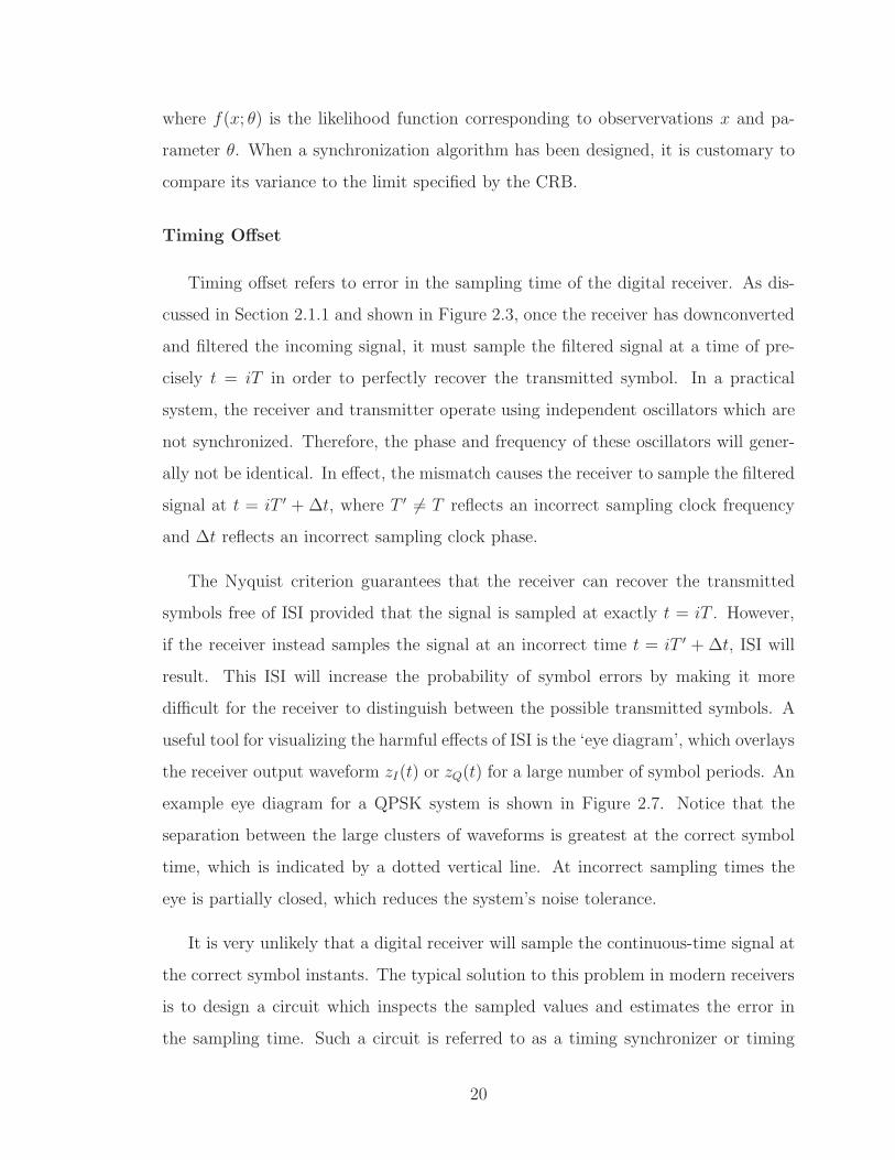
useful tool for visualizing the harmful effects of ISI is the ‘eye diagram’, which overlays

the receiver output waveform zI(t) or zQ(t) for a large number of symbol periods. An

example eye diagram for a QPSK system is shown in Figure 2.7. Notice that the

separation between the large clusters of waveforms is greatest at the correct symbol

time, which is indicated by a dotted vertical line. At incorrect sampling times the

eye is partially closed, which reduces the system’s noise tolerance.

It is very unlikely that a digital receiver will sample the continuous-time signal at

the correct symbol instants. The typical solution to this problem in modern receivers

is to design a circuit which inspects the sampled values and estimates the error in

the sampling time. Such a circuit is referred to as a timing synchronizer or timing

20

−1 −0.5 0 0.5 1−3

−2

−1

0

1

2

3

Sampling Time , t/T

Mat

ched

Filt

er O

utpu

t, z I(t

)

Figure 2.7 Eye diagram for QPSK system with α = .1.

recovery circuit. The timing error estimate is then passed to a digital interpolation

filter which processes the incoming samples to effectively resample the underlying

continuous-time signal at the correct sampling instants.

Frequency and Phase Offset

Another potential source of mismatch between the transmitter and receiver in

a digital communication system lies in the sinusoidal carriers used for upconversion

and downconversion in the transmitter and receiver respectively. Since these carriers

are generated from independent oscillators, there is some degree of disparity in their

frequency and phase. Mathematically, we can model the effect of this frequency and

phase offset by changing the arguments to the sinusoidal functions in the receiver

from 2πfct to 2π(fc+∆f)t+ φo. Using this model, the effect of phase and frequency

21

offset on the receiver’s downconversion process may be investigated:

vI(t) = y(t)2cos(2π(fc +∆f)t + φo)

= 2[wI(t)cos(2πfct)cos(2π(fc +∆f)t+ φo)

= + wQ(t)sin(2πfct)cos(2π(fc +∆f)t + φo)]

= wI(t)cos(2π∆ft+ φo)− wQ(t)sin(2π∆ft+ φo) (2.16)

vQ(t) = y(t)2sin(2π(fc +∆f)t+ φo)

= 2[wI(t)cos(2πfct)sin(2π(fc +∆f)t+ φo)

= + wQ(t)sin(2πfct)sin(2π(fc +∆f)t+ φo)]

= wQ(t)cos(2π∆ft+ φo) + wI(t)sin(2π∆ft+ φo) (2.17)

Note that the double frequency components have been omitted from the final

step in equations (2.16) and (2.17) due to the fact that they will be immediately

removed by the receiver’s matched filter. Clearly, frequency and phase offset cause

the received constellation points to rotate. In the case of phase offset, there is a single

initial rotation of φo radians, whereas frequency offset causes the constellation to spin

at a constant rate of 2π∆fT radians per symbol. These two effects may be seen in

Figure 2.8, which shows the received constellation points for 1000 transmitted QPSK

symbols with a phase offset of π/8 radians and a frequency offset of 10−4 ∗ 2π radians

per symbol.

It is apparent from Figure 2.8 that frequency and phase offset complicate the task

of the receiver, as the modulation scheme relies upon the angle of the received con-

stellation points to convey significant information. In order to make correct decisions,

the receiver must be able to estimate the phase and frequency offset so that it may

compensate for them by performing a derotation internally. Consequently, the design

and analysis of a frequency offset estimator for DOCSIS upstream channels is one of

the major goals of this thesis.

22

−1 −0.5 0 0.5 1−1

−0.5

0

0.5

1

Real Part of Received Signal, zI(kT)

Imag

inar

y P

art o

f Rec

eive

d S

igna

l, z Q

(kT

)Received symbolsExpected symbols

Figure 2.8 Received constellation points for 1000 QPSK symbols with ∆f = 10−4

and φo = π/8.

Channel Echoes

The design of a DOCSIS-based cable network is such that many CMs are connected

to the same physical cable network which eventually connects back to the headend.

Consequently, when a CM transmits on an upstream channel, its signal travels across

the network not only to the headend, but also to a potentially large number of CMs.

Given that the signal is reaching such a large number of devices, there is a relatively

high probability that some of the devices may not be perfectly impedance-matched

to the channel. The result of such a mismatch is that a portion of the transmitted

signal will be reflected back onto the cable and eventually to each of the connected

devices. Due to this phenomenon, the CMTS will not receive just a single copy of the

transmitted signal. Rather, it will receive multiple delayed copies of the transmitted

signal, each having different attenuation values and phase shifts. These reflected

23

Figure 2.9 Linear filter channel model used to represent effect of echoes.

signals are known as echoes or micro-reflections.

The effect of echoes on the signal received by a digital demodulator may be mod-

eled as the application of a linear filter hc(t) to the transmitted signal, as shown in

Figure 2.9. Note that in the model, the channel filter is applied prior to the addition

of AWGN.

When the distorted signal is processed at baseband inside the receiver, the con-

tinuous time channel filter may be modeled as an equivalent complex baseband filter

operating at the symbol rate. The coefficients of this filter may be determined for a

specific set of echoes by summing delayed and shifted copies of the combined impulse

responses of the transmitter and receiver shaping filters in order to generate an overall

impulse response. The linear filter coefficients may then be determined by sampling

the overall impulse response at the symbol rate, as shown in Figure 2.10.

To generate Figure 2.10, a single echo with an attenuation of 10dBc, a delay of

0.5T seconds, and a phase rotation of π radians has been applied to the signal. When

the echo-laden signal is sampled at the symbol rate, the samples indicated by large

dots are obtained. These samples determine the equivalent channel impulse response

for this scenario, which turns out to be: −.001z4+.0129z3−.0274z2+.0587z1+.8016−.1984z−1 + .0587z−2 − .0274z−3 + .0129z−4. Notice that the Nyquist ISI criterion is

not fulfilled when the echoes are present, highlighting the fact that the typical effect

of channel echoes is to add ISI to the signal. A constellation plot illustrating the

impact of this ISI may be seen in Figure 2.11.

The echo characteristics of the DOCSIS upstream channel are unique to each

24

−4 −2 0 2 4−0.4

−0.2

0

0.2

0.4

0.6

0.8

1

Time, t/T

Am

plitu

de

TransmittedEchoReceived

Figure 2.10 Effect of an echo on received baseband signal.

individual user. Additionally, new CMs are occasionally connected to the network,

while old CMs are periodically removed from the network. Each of these changes will

naturally cause the echoes present in the DOCSIS upstream channel to change over

time.

In this thesis, a channel model based on the DOCSIS standard [2] will be used.

The model allows for up to three echoes, with specifications as shown in Table 2.1

below:

Table 2.1 Echo channel model.

Relative Amplitude (dBc) Echo Delay (sym) Echo Phase (rad)

-10 Uniform (0 → 2.5) Uniform (0 → 2π)

-20 Uniform (0 → 5) Uniform (0 → 2π)

-30 Uniform (0 → 7.5) Uniform (0 → 2π)

In order for the upstream demodulator to properly recover the transmitted sym-

25

−1 −0.5 0 0.5 1−1

−0.8

−0.6

−0.4

−0.2

0

0.2

0.4

0.6

0.8

1

Real Part of Received Signal, zI(kT)

Imag

inar

y P

art o

f Rec

eive

d S

igna

l, z Q

(kT

)

Figure 2.11 ISI seen in QPSK constellation due to echo.

bols, it is necessary to remove some of the ISI from the received signal. Since the

characteristics of the upstream channel are not known a priori, it is necessary for the

demodulator to detect and compensate for the ISI on the fly. An adaptive equalizer

is particularly well-suited for this task, as will be discussed in Chapter 5.

2.2 MAC Layer Control

2.2.1 Overview

The overall network management for upstream DOCSIS channels is performed by

the media access control (MAC) layer of the CMTS. Although the detailed operation

of the MAC is outside the scope of this research, an overview of the basic principles

involved in the control of upstream channels is useful to provide context for the

remainder of the document.

26

In order to allow multiple users to transmit data to the headend via a single up-

stream channel, recent versions of the DOCSIS standard permit two multiple access

schemes: time division multiple access (TDMA) and synchronous code division mul-

tiple access (S-CDMA). Each upstream channel in a cable network must be using one

of these two multiple access schemes. Note that it is possible for these two schemes

to coexist on separate upstream channels within the same cable network. In TDMA

mode, the entire channel is allocated to a single user for a period of time. The users

take turns transmitting short bursts of data across the channel. In contrast, S-CDMA

mode allows multiple users to transmit data over the channel simultaneously using

orthogonal codes. The orthogonality of these codes ideally permits the CMTS to

correctly recover each of the transmitted data streams without any cross-user inter-

ference.

The goal of the present research is to develop synchronization algorithms for the

DOCSIS TDMA mode. Consequently, the remainder of this thesis will exclusively

focus on TDMA.

Each TDMA upstream channel is broken up into a sequence of timeslots by the

CMTS MAC. These timeslots, each of which corresponds to an upstream transmission

opportunity, are called minislots in the standard. The minislots are synchronized to

an extremely accurate 10.24MHz reference clock stored in the headend. The CMTS

keeps a count of the number of reference clock edges in a reference counter and

periodically transmits this count value to the CMs in a synchronization message via

a downstream channel. Like the CMTS, each CM contains a 10.24MHz clock that

drives its own reference counter. The value of this local reference counter is updated

to match the value transmitted by the CMTS reference counter to correct for drift

caused by differences between the two 10.24MHz clocks. This allows each CM within

the network to maintain a relatively accurate timebase.

The CMTS MAC layer is responsible for scheduling minislots on the upstream

channels and allocating these minislots to the individual CMs. In doing so, the MAC

layer attempts to maximize network throughput and minimize the latency experienced

27

Figure 2.12 An example of upstream bandwidth allocation using minislots.

by each user while ensuring an equitable distribution of network resources. Although

the the design of such a scheduling algorithm is clearly a difficult and important

problem, it is not of interest in the present document. Once the MAC layer has

decided upon the allocation of some number of minislots for an upstream channel, it

broadcasts a bandwidth map message to all of the CMs via a downstream channel

in order to inform the CMs of this allocation. Figure 2.12 provides an example of a

simple bandwidth allocation. Note that all of the minislots in the figure are defined

based on the value contained in the CMTS reference clock counter, which holds a

value of N at the start-time of minislot M .

As suggested in Figure 2.12, there are two main types of packets which are trans-

mitted across DOCSIS upstream channels: ranging packets and traffic mode packets.

These two packet types will be discussed in detail in Sections 2.2.2 and 2.2.3.

2.2.2 Ranging Mode

As discussed in Section 2.1.2, there are a large number potential impairments

which complicate the use of DOCSIS upstream channels. Fortunately, the CMs have

the capacity to correct many of these if given proper instruction by the CMTS. The

purpose of ranging mode is to allow the CMTS to measure certain parameters in a

controlled environment and to verify that the transmissions from a given CM may

be acceptably received. A CM must enter ranging mode upon initially connecting to

28

Figure 2.13 A spatial distribution of CMs can result in a large variation in message

transit times.

the network. Thereafter, each CM will be periodically instructed by the CMTS to

re-range in order to ensure the reliability of the upstream channel. Typically, each

modem is re-ranged every one to two minutes.

The most important of the transmission parameters which must be measured in

ranging mode is the timing offset of a CM. As discussed in Section 2.2.1, each CM

attempts to use the information received from synchronization messages on a down-

stream channel to correct the local reference counter. Unfortunately, this system does

not work perfectly since the CMs are spread out over a geographical area of up to

150 kilometres. Given this wide spatial distribution of CMs, a synchronization mes-

sage containing the same timestamp can arrive at two different CMs at significantly

different times, as shown in Figure 2.13.

Due to this phenomenon, the transmission of synchronization messages alone is

not enough to ensure the CMs are able to time their transmissions to arrive at the

CMTS at precisely the start of the appropriate minislots. Ranging packets are used

to measure the transit time prior to allowing a CM to enter traffic mode and begin

transmitting ‘real’ data. In order to do so, the CMTS allocates a number of minislots

for ranging opportunities, during which CMs attempt to transmit a known packet at

a known time. The measured transit time is then sent to the CM via a downstream

transmission. When allocating minislots, the CMTS ensures that ranging minislots

29

Figure 2.14 Ranging minislots provide a buffer to allow for CM timebase variability.

are much larger than is strictly necessary to transmit the necessary ranging packet,

as seen in Figure 2.14. This ensures that a transmission from a CM with an incorrect

timebase will not overlap into the next minislot and interfere with another user’s

transmission. By searching through the ranging packet for a specific pattern, the

CMTS is able to deduce the propagation delay of the ranging CM.

In addition to timing recovery, a number of other important transmission param-

eters are generally optimized by the CMTS during ranging:

Frequency offset: As discussed in Section 2.1.2, a frequency offset causes the re-

ceived constellation to spin, making the demodulator’s task much more difficult.

It is desirable to reduce the frequency offset associated with each CM, especially

when higher order QAM constellations are to be used. The CMTS measures the

frequency offset for each ranging packet and instructs the transmitting CM to

adjust its carrier frequency in order to minimize the frequency offset in future

packets.

Transmit power: In order to keep the network running smoothly, it is desirable

for the power level received by the CMTS to be relatively consistent between

CMs. Transmit power is measured during a ranging packet so that the power

of the transmitting CM may be adjusted as necessary to achieve this goal.

Channel echoes: As mentioned in Section 2.1.2, echoes are often present on DOC-

30

Figure 2.15 Structure of pre-equalizer in DOCSIS upstream transmitter.

SIS upstream channels. These echoes produce ISI, complicating the demodu-

lation process. Although it is possible to remove the ISI in the demodulator

through the use of an adaptive equalizer, the process of adapting the equalizer

coefficients requires the transmission of a large number of symbols, which would

add a great deal of overhead to each upstream packet. The solution presented

in the DOCSIS standard is to place a pre-equalizer in the CM and allow the

CMTS to determine the coefficients of this equalizer. The equalizer in the CM

has a linear structure, as shown in Figure 2.15. Each ranging packet contains

the necessary overhead for the CMTS to determine the equalizer coefficients

necessary to cancel the unique ISI produced by the channel from the transmit-

ting CM to the CMTS. Using these coefficients, each CM is able to pre-equalize

its transmissions in order to cancel the channel ISI so that the signal reaching

the CMTS is ideally ISI-free.

After each ranging packet, the CMTS will send a ranging response packet back to

the CM on a downstream channel. The ranging response packet contains information

regarding all of the estimated parameters discussed above. Additionally, the response

will indicate whether further ranging is necessary. If the ranging packet was received

successfully and the CM is matched to the channel acceptably well, the CM is reg-

istered with the CMTS and instructed to exit ranging mode and enter traffic mode.

Alternatively, if the ranging packet was not received sufficiently well or if any of the

transmitter parameters discussed above require significant adjustment, the CM is re-

31

quired to update its parameters and send another ranging packet in an appropriate

minislot.

2.2.3 Traffic Mode

In traffic mode, a CM uses upstream bandwidth in order to transmit ‘real’ data.

In this mode, transmissions are relatively free of impairments, since the CMs are re-

ranged often enough to ensure that is the case. Thus, it is unnecessary for the CMTS

to measure and correct transmitter inaccuracies in traffic mode. As a result, there is

typically much less overhead in traffic mode packets than ranging packets.

The overall goal of the CMTS is to maximize the amount of data flowing through

the upstream channels in order to provide the highest possible level of service to users

of the cable network. In order to achieve this goal, the DOCSIS MAC is responsible

for defining and allocating minislots to individual CMs in response to bandwidth re-

quests. For each individual minislot allocation, the MAC must also select appropriate

physical layer transmission parameters, including the constellation, error control cod-

ing parameters, and interleaving parameters. These parameters must be selected on

a per-user basis in order to optimize the throughput of each minislot. Once again, the

algorithms which the MAC uses to complete this scheduling and parameter selection

task are intriguing and complex, but not directly relevant to the current discussion.

Over time, the timing offset, frequency offset, channel echoes, and received power

corresponding to each CM may slowly change, causing degradations to traffic mode

performance. To combat this phenomenon, the CMTS periodically sends the modems

back into ranging mode to resynchronize. Additionally, the CMTS continues to mon-

itor each of the synchronization parameters during traffic mode. In the event that

any of these parameters deviates beyond an acceptable tolerance level, the CMTS

instructs the CM in question to return to ranging mode in order to re-measure and

then re-optimize the transmission parameters.

This research is focused on synchronization algorithms for the TDMA DOCSIS

upstream channel, so the remainder of the document will concentrate on ranging

32

mode packets.

33

3. Demodulator Architecture

3.1 High-Level Architecture

The general structure of the proposed CMTS upstream receiver is shown in Fig-

ure 3.1. As shown in the figure, the input RF signal is first passed to an analog

front end module, which bandlimits the incoming signal. The signal is then digitized

through the use of an analog to digital converter (ADC) and passed to an FPGA for

processing. Inside the FPGA, the sampled signal is first passed to a digital front end,

which downconverts and downsamples the signal to reduce the computational burden

on the digital demodulator. The output of the digital front end, which is a complex

baseband signal, is sent to the digital demodulator. The demodulator recovers the

data and passes the results to the MAC. Note that the demodulator and both front

ends are controlled by tuning and channel information from the MAC layer.

The functionality and design of the analog and digital front end blocks will be

briefly discussed prior to a more detailed overview of the structure of the digital

demodulator, which is the focus of this research.

Figure 3.1 High level structure of upstream demodulator.

34

Figure 3.2 Block diagram of complete band sampling analog front end.

3.1.1 Analog Front End

The goal of the analog front end is to generate an accurate and high-resolution

digital representation of the incoming analog signal. In order to do so, any frequency

components in the input signal which are outside the valid DOCSIS upstream band

of 5-85MHz must first be removed with a bandpass filter. However, the design of the

remainder of the analog front end is not so straightforward. Two potential structures,

each of which has some compelling advantages, will be considered.

The first option is to sample the entire upstream frequency band using a very

high-speed and high-resolution ADC. The analog front end for this technique, which

will be referred to as ‘complete band sampling’ (CBS), is depicted in Figure 3.2.

The main advantage of the CBS design is seen when multiple demodulators are

placed in a single FPGA. In such a scenario, only one analog front end is necessary

since the sampled signal simultaneously contains all of the upstream channels. Ad-

ditionally, this design uses a minimum amount of analog RF circuitry, which may be

beneficial from a reliability standpoint, given the unit-to-unit variability associated

with analog circuits.

The downside to the CBS structure is that it requires a very high quality ADC. In

order to sample the entire 5-85MHz frequency spectrum without any aliasing issues,

the sampling frequency must be at least 85MHz ∗2 = 170MHz. Additionally, there

may be significant variability in power between upstream channels, making some of

the lower-powered channels more difficult to receive. To combat this problem, the

ADC must provide a very high quality output signal, which necessitates an expensive

ADC.

35

Figure 3.3 Block diagram of band-selective sampling analog front end.

A second option for the design of the analog front end is to sample only a small

portion of the upstream frequency band. In order to use this approach, which will

be referred to as ‘band-selective sampling’ (BSS), additional filters must be used to

bandlimit the analog signal prior to the analog-to-digital conversion process in such a

way that the channel of interest is retained. One typical method for bandlimiting the

analog signal utilizes an intermediate frequency (IF) tuner, as shown in Figure 3.3.

The IF tuner mixes the desired channel to a specific intermediate frequency (com-

monly 44MHz) and then applies a narrowband filter to the IF signal. The filter is

selected to be just slightly wider than the widest possible input channel, likely around

6MHz in the case of DOCSIS upstream channels. The narrowband output from the

filter is passed to an ADC and then to the FPGA.

Compared to the CBS model, the ADC in a BSS architecture can use a much

lower sampling frequency for its ADC without experiencing any aliasing. Also, since

the output of the IF tuner is a narrowband signal containing only one upstream

channel, it is possible to apply AGC to only the channel of interest, meaning that

the full resolution of the ADC is used to represent the desired channel. Thus, less

resolution is needed in the ADC for BSS than in CBS, where the AGC is unable to

perform scaling on a single channel. Due to the less stringent ADC requirements, it

is expected that the hardware cost of a BSS front end would be significantly less than

that of a CBS front end. However, since the CBS samples only a single upstream

36

Figure 3.4 Block diagram of digital front end for upstream demodulator.

channel, it is necessary to use one BSS for each demodulator.

3.1.2 Digital Front End

Regardless of which analog front end architecture is used, the input to the FPGA

will be sampled at a rate which is significantly higher than the symbol rate of the

upstream channel of interest. For the symbol recovery block to do its job efficiently,

the sampling rate of the digital signal should be reduced to be two, three, or four

times the symbol rate of the upstream channel in question. The symbol recovery

design discussed in this thesis operates using four samples per symbol. Also, the

symbol recovery circuit operates on the complex baseband equivalent of the upstream

channel. Thus, it is necessary for the digital front end to downconvert the input signal

to baseband.

Conceptually, the structure of the digital front end is illustrated in Figure 3.4.

Note that input from the MAC is necessary in order for the digital front end to know

what frequency to mix the incoming signal with and also to know by what factor

the baseband signal should be downsampled. In order to prevent aliasing, a low pass

filter must be applied to the downconverted signal prior to downsampling. Polyphase

finite impulse response (FIR) filters are a good choice for this purpose, as they are

relatively inexpensive to implement in modern FPGAs.

Recent developments in digital signal processing suggest that the digital front

37

end could be constructed more economically using a fast-Fourier-transform-based

structure, rather than that of Figure 3.4. However, the detailed design of the digital

front end is outside the scope of this document.

3.1.3 Symbol Recovery

The symbol recovery module accepts a complex baseband input signal from the

digital front end and recovers the symbols transmitted on the upstream channel by the

CM. In order to demodulate the upstream transmission, the symbol recovery module

must first filter the incoming signal with a filter that is matched to the transmitter’s

pulse shaping filter. For DOCSIS upstream channels, the transmitter’s pulse shaping

filter is specified as having a SRRC impulse response with α = 0.25.

As discussed in Section 2.1.2, there are a number of impairments present in the

DOCSIS upstream channel which, left uncorrected, will significantly hinder the per-

formance of the symbol recovery circuit. Thus, prior to making a decision regarding

which symbols have been transmitted, the demodulator must first attempt to syn-

chronize with the transmitter in order to compensate for impairments in the filtered

signal. In order to facilitate this synchronization, a known sequence of symbols is

transmitted at the beginning of each upstream packet, as shown in Figure 3.8. These

symbols, collectively referred to as the preamble, are selected by the CMTS so as to

permit the best possible impairment correction performance.

The design of the synchronization circuits used for impairment detection and

correction is one of the main challenges in the design of a DOCSIS upstream receiver.

In general, there are two main categories of synchronization algorithms: feedback

systems and feedforward systems.

Feedback Synchronizers

In feedback synchronizers, the incoming signal is passed into a parameterized com-

pensation device, the purpose of which is to adjust the signal in order to compensate

for errors in the parameter of interest (timing, frequency, or phase). The output of the

38

Figure 3.5 Typical structure of a feedback synchronizer.

compensator is passed to an error detection block, which indicates the approximate

magnitude of the error remaining in the compensated signal, as shown in Figure 3.5.

This error signal is passed through a loop filter in order to reduce jitter, then fed

back to the parameterized compensator. Over time, if the loop is working correctly,

the error in the compensator’s output should approach zero.

Note that a synchronization circuit operating in feedback mode does not actually

estimate the error in the parameter as seen at the demodulator input. Rather, the

error in the compensated output is detected. When the error at the output of the

compensator is large, feedback synchronization circuits tend to suffer from nonlinear-

ity issues. To prevent the nonlinearity of the estimator from having an adverse effect

on the convergence of a feedback estimator, the loop gain must be made small. The

result is that feedback estimators can be relatively slow to converge. While this is not

a problem for systems utilizing continuous transmission such as DOCSIS downstream

channels, it is not ideal for burst channels, such as those used for DOCSIS upstream

communication [9].

Feedforward synchronizers

The typical structure of a feedforward estimator is shown in Figure 3.6. As shown

in the figure, the estimation portion of a feedforward synchronizer operates on the

39

Figure 3.6 Typical structure of a feedforward synchronizer.

input signal, rather than the output of the compensator. In contrast to a feedback

estimator, the estimation module in a feedforward configuration is responsible for

estimating the overall value of the parameter at the synchronizer’s input. This infor-

mation is then passed on to the compensation block.

Since stability is not a concern in feedforward systems, feedforward synchronizers

are able to avoid the loop gain and nonlinearity issues faced by feedback synchronizers.

The result is that feedforward synchronizers tend to converge more quickly than do

feedback synchronizers. Due to this faster convergence, feedforward synchronizers are

well-suited to burst applications, such as DOCSIS upstream channels.

It has been shown in [13] that feedback circuits can be used effectively in a DOC-

SIS upstream demodulator. However, the current research focuses on feedforward

techniques, as they are a natural fit for DOCSIS upstream channels. The overall

structure of the proposed symbol recovery module is shown in Figure 3.7.

In the most straightforward implementation, the preamble symbols are broken up

into four distinct blocks, each of which is used by one of the impairment-correcting

circuits:

40

Figure 3.7 High level block diagram of symbol recovery module.

Figure 3.8 The structure of an upstream packet.

The general signal flow through the symbol recovery module is:

1. Using the preamble symbols, the symbol recovery module first estimates the

timing error in the upstream transmission. Using an interpolator and down-

sampler, the effective sampling times of the digital signal are modified so that

the demodulator has access to samples corresponding to the correct symbol

times.

2. Next, the frequency recovery module acts on the downsampled signal in order to

estimate any carrier frequency offset which may be present in the channel using

a specialized frequency recovery preamble. The estimated carrier frequency

error is removed from the signal by a despinner.

41

3. A third portion of the preamble is used by the phase recovery circuit in order

to detect a rotation of the constellation by a fixed angle. The resulting phase

error estimate is passed to a derotator inside the equalizer for correction.

4. The fourth and final section of the preamble is a training sequence for an equal-

izer. Using this preamble, the equalizer applies an adaptive algorithm to de-

termine a set of filter coefficients which is able to compensate for the micro-

reflections present in the upstream channel.

Note that the timing, frequency, and phase estimators operate only during the

preamble portion of the packet. Once an estimate of the relevant parameter has been

obtained from the preamble symbols, an appropriate correction is applied for the

remainder of the packet. In contrast, the equalizer is able to continually adapt its

taps throughout the entire packet.

One common metric used to analyze the performance of a demodulator is Mod-

ulation Error Ratio (MER), which measures the amount of error in the received

constellation points after the demodulator has attempted to compensate for the im-

pairments. Mathematically, MER is defined as follows:

MER(dB) = 10 ∗ log10

(Es

1N

∑Nj=1 |ej|2

)(3.1)

where Es is the average symbol energy and ej is the error in the jth received symbol.

The choice of a preamble for each of the impairment estimation circuits can have

a significant impact on the performance of each of the circuits. Certain patterns of

preamble symbols can be used to maximize the probability of accurate estimates.

The length of the sequence used to estimate the transmission impairments present in

the upstream channel will also affect the performance of the impairment estimators.

Longer preamble sequences permit more accurate estimates, but are less efficient from

a data throughput point of view. Additionally, it is desirable if the same preamble can

be used for multiple synchronization functions simultaneously. This would allow the

overall preamble sequence to be shortened, increasing the efficiency of the channel.

42

Given these considerations, the selection of an appropriate preamble sequence will be

one of the major topics of this document.

The remaining chapters of this thesis will develop novel frequency recovery, phase

recovery, and equalization circuits that use modest amounts of FPGA resources, yet

perform at near optimum levels.

43

4. Frequency and Phase Recovery

4.1 Introduction

As discussed in Section 2.1.2, frequency and phase differences between the carriers

used for upconversion and downconversion cause the received constellation to spin

and rotate, respectively. Any unexpected rotation is problematic in QAM systems,

as the transmitted data is encoded in both the amplitude and phase of the sinusoidal

carrier. Thus, in order to reliably recover the transmitted symbols, it is necessary to

estimate and correct these offsets. This chapter discusses the design of the circuits

which perform this task, known as the frequency and phase recovery modules.

As previously seen in Figure 3.7, the frequency recovery circuit operates upon the

downsampled output of the timing recovery interpolator. Assuming that the timing

recovery circuit is working correctly, the digital signal presented to the frequency

recovery circuit has exactly one sample per symbol, with the sample being taken at

the correct sampling time. Ignoring any potential ISI for the time being, the input

signal to the frequency recovery module during the preamble portion of the packet

may be written as follows:

yf [n] = anej(∆ωn+φo) + η[n] ; 0 ≤ n ≤ N − 1 (4.1)

where an is the complex transmitted symbol chosen from a unit-energy QPSK con-

stellation, ∆ω is the frequency offset, and φo is the phase offset. During the preamble,

it is possible for the receiver to remove the angle modulation on this complex sinu-

soid by multiplying with the complex conjugate of the transmitted symbol, a∗n, which

44

reduces the expression to:

yu[n] = ej(∆ωn+φo) + ηr[n] ; 0 ≤ n ≤ N − 1 (4.2)

where ηr[n] is a rotated version of the noise and has the same statistics as η[n], which

are a mean of 0 and a variance of σ2.

For the reasons discussed in Section 3.1.3, the frequency and phase estimators are

restricted to the use of data-aided feedforward algorithms in this research.

4.2 Performance Limits

Before proceeding with the development of the frequency and phase recovery al-

gorithms, the performance limits for such algorithms are investigated. These limits,

in the form of CRBs, will provide a reference point against which the proposed algo-

rithms may be evaluated.

In order to find the CRB for a random vector ofNp parameters p = [p0 p1 . . . pNp−1]

to be estimated, the Fisher information matrix, denoted I(p), must first be calculated.

The entries of I(p) are determined by taking the expectation of partial derivatives of

the log-likelihood function as follows:

[I(p)]ij = E

[−∂

2lnfy(y; p)

∂pi∂pj

](4.3)

The CRB on the variance of each parameter pi may be read from a diagonal entry

of the inverse of the Fisher information matrix:

var(pi) ≥ [I−1(p)]ii (4.4)

From equation (4.2), it is clear that yu[n] is a complex Gaussian random variable with

a mean of ej(∆ωn+φo) and a variance of σ2. Since the noise ηr[n] is independent of

ηr[k] if k 6= n, the likelihood function for yu = [ yu[0], yu[1], . . . yu[N − 1] ] may be

expressed as:

fyu(yu; ∆ω, φo) =

(1

πσ2

)Ne

−1

σ2

∑N−1n=0 |yu[n]−ej(∆ωn+φo)|2 (4.5)

45

and the log-likelihood function is given by:

Λyu(yu) = ln(fyu(yu; ∆ω, φo)) = ln

(1

πσ2

)N− 1

σ2

N−1∑

n=0

∣∣yu[n]− ej(∆ωn+φo)∣∣2

= ln

(1

πσ2

)N−

1

σ2

N−1∑

n=0

(yu[n]yu[n]

∗ − yu[n]e−j(∆ωn+φo) − yu[n]

∗ej(∆ωn+φo) + 1)

(4.6)

Next, finding the required second partial derivatives of the log-likelihood function:

∂Λyu(yu)

∂∆ω=

−1

σ2

N−1∑

n=0

(yu[n]e

−j(∆ωn+φo)(jn)− yu[n]∗ej(∆ωn+φo)(jn)

)(4.7)

∂Λyu(yu)

∂φ0

=−1

σ2

N−1∑

n=0

(jyu[n]e

−j(∆ωn+φo) − jyu[n]∗ej(∆ωn+φo)

)(4.8)

∂2Λyu(yu)

∂∆ω2=

−1

σ2

N−1∑

n=0

(n2yu[n]e

−j(∆ωn+φo) + n2yu[n]∗ej(∆ωn+φo)

)(4.9)

∂2Λyu(yu)

∂∆ω∂φ0=

−1

σ2

N−1∑

n=0

(nyu[n]e

−j(∆ωn+φo) + nyu[n]∗ej(∆ωn+φo)

)(4.10)

∂2Λyu(yu)

∂φ20

=−1

σ2

N−1∑

n=0

(yu[n]e

−j(∆ωn+φo) + yu[n]∗ej(∆ωn+φo)

)(4.11)

Substituting the right hand side of equation (4.2) for yu[n] in equations (4.9),

(4.10), and (4.11), then taking the expectation yields:

E

[−∂

2Λyu(yu)

∂∆ω2

]=

1

σ2

N−1∑

n=0

(n2ej(∆ωn+φo)e−j(∆ωn+φo) + n2e−j(∆ωn+φo)ej(∆ωn+φo)

)

=2

σ2

N−1∑

n=0

n2 (4.12)

E

[−∂

2Λyu(yu)

∂∆ω∂φo

]=

1

σ2

N−1∑

n=0

(nej(∆ωn+φo)e−j(∆ωn+φo) + ne−j(∆ωn+φo)ej(∆ωn+φo)

)

=2

σ2

N−1∑

n=0

n (4.13)

46

E

[−∂

2Λyu(yu)

∂φ2o

]=

1

σ2

N−1∑

n=0

(ej(∆ωn+φo)e−j(∆ωn+φo) + e−j(∆ωn+φo)ej(∆ωn+φo)

)

=2

σ2

N−1∑

n=0

1 (4.14)

The expressions above can be simplified using the identities

N−1∑

n=0

n =(N − 1)N

2(4.15)

N−1∑

n=0

n2 =(N − 1)N(2N − 1)

6(4.16)

with the result:

E

[−∂

2Λyu(yu)

∂∆ω2

]=

(N − 1)N(2N − 1)

3σ2(4.17)

E

[−∂

2Λyu(yu)

∂∆ω∂φo

]=

(N − 1)N

σ2(4.18)

E

[−∂

2Λyu(yu)

∂φ2o

]=

2N

σ2(4.19)

Thus, the Fisher information matrix is:

[I(p)] =

(N − 1)(N)(2N − 1)

3σ2

(N − 1)(N)

σ2

(N − 1)(N)

σ2

2N

σ2

(4.20)

and its inverse is:

[I−1(p)

]=

1

det(I(p))

2N

σ2

−(N − 1)(N)

σ2

−(N − 1)(N)

σ2

(N − 1)(N)(2N − 1)

3σ2

(4.21)

where

det(I(p)) =2N2(N − 1)(2N − 1)

3σ4− N2(N − 1)2

σ4

=1

3σ4

[2N2(N − 1)(2N − 1)− 3N2(N − 1)2

]

=N2(N2 − 1)

3σ4(4.22)

47

This reduces to

[I−1(p)

]=

6σ2

N(N2 − 1)

−3σ2

N(N + 1)

−3σ2

N(N + 1)

σ2(2N − 1)

N(N + 1)

. (4.23)

The CRBs on the variance of frequency and phase offset estimators may be read

from the inverse of the Fisher information matrix. Keeping in mind that E[|an|2] = 1

and E[|η|2] = σ2, the bounds may be expressed in terms of the signal-to-noise ratio

(SNR) rather than the noise variance by using the identity SNR = 1σ2.

var(∆ω) ≥[I−1(p)

]11

=6σ2

N(N2 − 1)=

6

N(N2 − 1)SNR(4.24)

var(φo) ≥[I−1(p)

]22

=σ2(2N − 1)

N(N + 1)=

2N − 1

N(N + 1)SNR(4.25)

4.3 Maximum Likelihood Estimators

The maximum likelihood technique is a common method for estimating a set of

parameters. This technique is very popular because it offers a straightforward method

of generating estimators which achieve the CRB for high SNRs and long observation

sequences. For this reason, the maximum likelihood technique is a logical place to

start a search for resource-efficient frequency and phase offset estimators.

As the name suggests, the maximum likelihood algorithm involves finding the

parameter values which maximize the likelihood function for the given set of obser-

vations. An estimator derived in this fashion is referred to as a maximum likelihood

(ML) estimator.

Since the natural logarithm function is monotonic, maximizing the log-likelihood

function is equivalent to maximizing the likelihood function. Given the exponential

nature of the likelihood function, the log-likelihood function is typically much easier

to work with than the original likelihood function. In order to maximize the log-

likelihood function, the most straightforward technique is to find the point at which

the derivative of the function with respect to the parameter of interest is zero. In

48

the case of multiple parameters, the joint ML estimator is found by solving for the

set of parameters that simultaneously set the partial derivatives with respect to each

parameter equal to zero.

The application of the maximum likelihood technique to the current task of esti-

mating the frequency and phase offsets starts with the log-likelihood function:

Λyu(yu) = ln(fyu(yu; ∆ω, φo)) = ln

(1

πσ2

)N− 1

σ2

N−1∑

n=0

∣∣yu[n]− ej(∆ωn+φo)∣∣2 (4.26)

The partial derivatives of the log-likelihood function with respect to ∆ω and φo are

given by equations (4.7) and (4.8). Setting the derivatives to 0 yields the equations:

0 =N−1∑

n=0

(−nyu[n]e−j(∆ωn+φo) + nyu[n]

∗ej(∆ωn+φo))

(4.27)

0 =

N−1∑

n=0

(−yu[n]e−j(∆ωn+φo) + yu[n]

∗ej(∆ωn+φo))

(4.28)

Unfortunately, in many cases, the ML approach does not yield a simple closed-

form expression for an estimator. The current problem appears to be such a case, as

it is not possible to solve equations (4.27) and (4.28) for ∆ω and φo. If computational

complexity and latency were not important considerations, it would be possible to

implement a maximum likelihood estimator by exhaustively evaluating the likelihood

function over the allowable parameter range. However, this type of approach is clearly

impractical for a resource-constrained FPGA-based demodulator.

Alternatively, it is possible to obtain closed-form expressions for ML frequency

and phase offset estimators by making certain approximations which are valid for

high SNRs. The details of this derivation are outlined in Appendix A. Unfortunately,

the estimators derived in this section are still too complex to implement economically

in an FPGA.

When the ML technique fails to yield a convenient estimator, it is necessary to

utilize alternate approaches to deriving an estimator. The design of such approaches

commonly relies upon intuition and mathematical heuristics. The following sections

49

will individually examine the tasks of frequency offset estimation and phase offset

estimation in this fashion.

4.4 Frequency Offset Estimator

4.4.1 Previous Work

The problem of estimating the carrier frequency of a burst digital signal has been

well-studied over the last half-century. Rife and Boorstyn laid the groundwork for

the field [27] by deriving the Cramer-Rao bounds (CRB) and maximum likelihood

estimators for the estimation of the amplitude, frequency, and phase of a single tone

from discrete-time observations. In [15], Tretter showed that a statistically efficient

estimator of the frequency of a noisy sinusoid may be generated using linear regression

techniques. An alternative CRB-achieving scheme, proposed by Kay in [16], exploits

the correlation between the phase of the incoming samples. Later, Luise and Reg-

giannini [17] used maximum likelihood techniques to derive a cost-effective frequency

recovery algorithm for high-SNR signals. One other notable estimator is that pro-

posed by Mengali and Morelli in [18], which has the advantage of a particularly large

estimation range.

The amount of published work in the area of frequency estimation specifically for

DOCSIS upstream channels is relatively limited. In [28], Wang and Speidel suggested

a technique based upon the measurement of the phase angle of the output of a pream-

ble detector. Most recently, Kim et al. [12] surveyed the literature and concluded that

Mengali and Morelli’s technique is well-suited to the upstream channel.

Despite all of this fine work, DOCSIS upstream channels present one key issue

which does not appear to have been analyzed in the literature: the effect of micro-

reflections or ‘echoes’. Significant ISI in the received signal due to micro-reflections

tends to bias the carrier frequency estimators discussed above, reducing their suit-

ability for use in a DOCSIS upstream receiver.

Going forward, a data-aided frequency estimation algorithm is developed that is

50

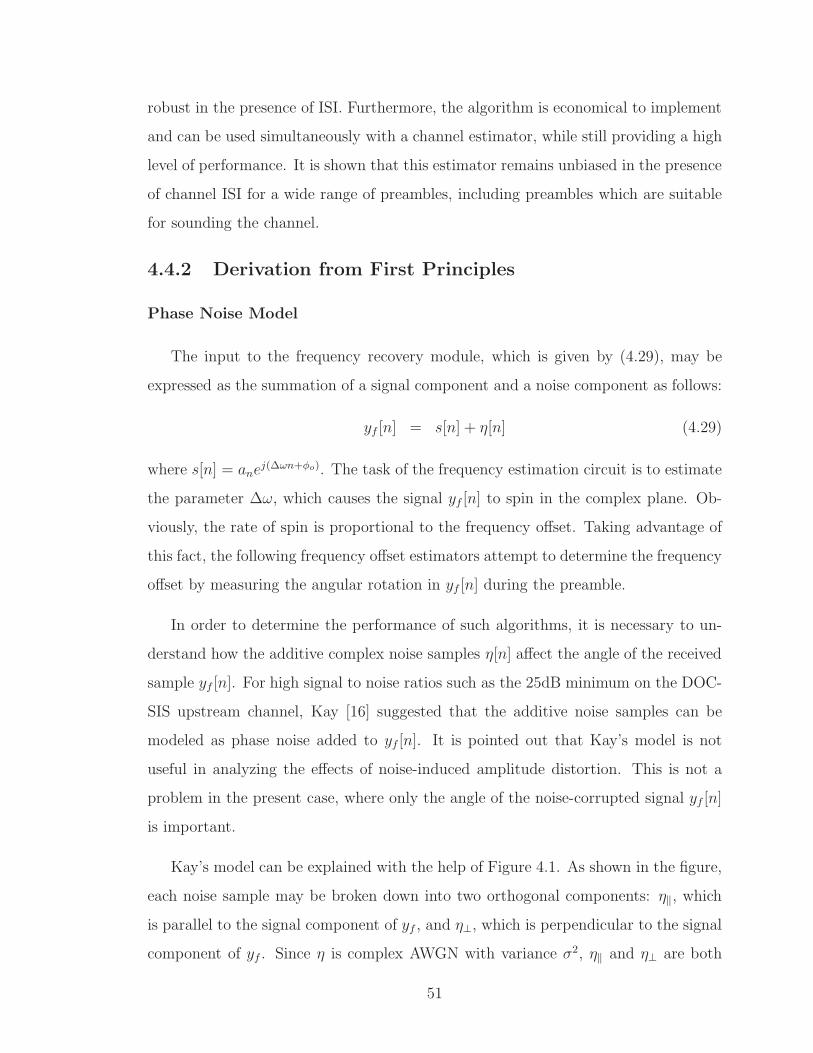
robust in the presence of ISI. Furthermore, the algorithm is economical to implement

and can be used simultaneously with a channel estimator, while still providing a high

level of performance. It is shown that this estimator remains unbiased in the presence

of channel ISI for a wide range of preambles, including preambles which are suitable

for sounding the channel.

4.4.2 Derivation from First Principles

Phase Noise Model

The input to the frequency recovery module, which is given by (4.29), may be

expressed as the summation of a signal component and a noise component as follows:

yf [n] = s[n] + η[n] (4.29)

where s[n] = anej(∆ωn+φo). The task of the frequency estimation circuit is to estimate

the parameter ∆ω, which causes the signal yf [n] to spin in the complex plane. Ob-

viously, the rate of spin is proportional to the frequency offset. Taking advantage of

this fact, the following frequency offset estimators attempt to determine the frequency

offset by measuring the angular rotation in yf [n] during the preamble.

In order to determine the performance of such algorithms, it is necessary to un-

derstand how the additive complex noise samples η[n] affect the angle of the received

sample yf [n]. For high signal to noise ratios such as the 25dB minimum on the DOC-

SIS upstream channel, Kay [16] suggested that the additive noise samples can be

modeled as phase noise added to yf [n]. It is pointed out that Kay’s model is not

useful in analyzing the effects of noise-induced amplitude distortion. This is not a

problem in the present case, where only the angle of the noise-corrupted signal yf [n]

is important.

Kay’s model can be explained with the help of Figure 4.1. As shown in the figure,

each noise sample may be broken down into two orthogonal components: η‖, which

is parallel to the signal component of yf , and η⊥, which is perpendicular to the signal

component of yf . Since η is complex AWGN with variance σ2, η‖ and η⊥ are both

51

Real Axis

ImaginaryAxis

s

yf

ηη‖

η⊥

ψ

Figure 4.1 Modeling AWGN as phase noise.

Gaussian random variables with identical variances of σ2/2. Taking advantage of the

noise decomposition, the phase error, denoted as ψ, may be found using a simple

trigonometric function:

ψ = tan−1

(η⊥|s|

)(4.30)

For large signal to noise ratios, the magnitude of the signal component of yf will

be much larger than η⊥, so the approximation tan(x) ≈ x may be applied, yielding

the result

ψ ≈ η⊥|s| radians (4.31)

DOCSIS 3.0 upstream channels always use QPSK modulation for the preamble,

so |s| has a constant value. Thus, the variance of the phase noise ψ is equal to:

σ2ψ = E[(ψ − E[ψ])2] = E

[(η⊥|s| − E

[η⊥|s|

])2]

radians2

=E[η2⊥]

|s|2 =σ2

2|s|2 =1

2SNRradians2 (4.32)

52

Thus, for large SNRs, the input signal to the frequency recovery circuit may be

modeled as:

yp[n] = anej(∆ωn+φo+ψ[n]) (4.33)

The Estimator - Insight and Performance

Preamble-based frequency offset estimators typically operate by measuring and

combining the angular differences between a set of incoming samples. Perhaps the

most basic technique computes the angular difference between two successive samples.

The frequency offset is then estimated as this angular difference. The heart of this

simple technique is a circuit known as a differential detector. A differential detector

multplies the current input sample by the complex conjugate of the previous sample.

In mathematical terms, its output is:

ydd[n] = y[n]y∗[n− 1] (4.34)

using the phase noise approximation given by (4.33) has:

ydd[n] ≈ anej(∆ωn+φo+ψ[n])a∗n−1e

−j(∆ω(n−1)+φo+ψ[n−1])

≈ ana∗n−1e

j(∆ω+ψ[n]−ψ[n−1]) (4.35)

The phase of the output has three terms: ∆ω, ψ[n], and ψ[n − 1]. The latter two

terms correspond to the phase noise. In practice, the angle of ydd[n] is computed

through the use of either a coordinate rotation digital computer (CORDIC) inverse

tangent circuit [29] or a look-up table. Neglecting any error introduced by the angle

computation device, this simple estimator may be expressed as:

∆ωn−1,n = ∆ωsimple[n] = arg(ydd[n])

= arg(ana∗n−1) + arg(ej(∆ω+ψ[n]−ψ[n−1]))

= arg(ana∗n−1) + ∆ω + ψ[n]− ψ[n− 1] (4.36)

where the subscripts on ∆ωn−1,n indicate that the inputs to the differential detector

correspond to samples n− 1 and n. The sequence of symbol values is known during

the preamble, so the contribution of arg(ana∗n−1) can be removed. Since the sampling

53

rates of sequences y[n] and ydd[n] are equal to the symbol rate, the units of the

estimator given by (4.36) are radians/symbol. Keeping in mind that the phase noise

ψ[n] is a sequence of i.i.d. random variables with mean and variance equal to 0 and

1/(2 · SNR) respectively, it is clear that the estimator of (4.36) is unbiased and that

the variance of ∆ωsimple[n] is equal to 1/SNR in units of (radians/symbol)2.

In order to produce more precise estimates, one obvious approach is to average

M estimates from the simple estimator of (4.36), yielding the following estimator:

∆ωavg =1

M

M∑

n=1

∆ωn−1,n

=1

M

M∑

n=1

(∆ω + ψ[n]− ψ[n− 1])

= ∆ω +ψ[M ]

M− ψ[0]

M(4.37)

An alternative approach to improving the simple estimator is to use a differential

detector with a larger differential delay of M samples. Such an estimator can be

expressed as:

∆ωn−M,n = ∆ωwide =1

Marg(y[n]y[n−M ]∗)

= ∆ω +ψ[M ]

M− ψ[0]

M(4.38)

Interestingly, this M−wide differential approach yields the same result as the aver-

age of M 1−wide differential detector outputs. The estimators of equations (4.37)

and (4.38) produce the same output, so from a theoretical point of view, theM−wide

differential and average of M 1−wide implementations may be used interchangeably.

However, from an implementation perspective, they are quite different, as discussed

in Section 4.4.2.

It is apparent from (4.37) that the average ofM 1−wide estimators, ∆ωavg, is itself

an unbiased estimator that has variance 1M2SNR

, which is lower than the variance of

the simple estimator by a factor of M2. Equation (4.37) also indicates that only the

phase noise at samples 0 andM corrupt the estimator’s output. Since the phase noise

54

Figure 4.2 The set of independent estimators which are combined in the decreasing

average-length technique.

sequence ψ[n] is iid, estimators which start and end on different samples will produce

independent estimates. That is, two estimators that have four different endpoints are

independent.

For anN symbol preamble. it is possible to construct a set ofN/2 (or (N−1)/2 for

N odd) independent averaging estimators by starting and stopping the averaging on

different samples. A composite estimator with lower variance can then be constructed

by weighting and summing these N/2 or (N − 1)/2 independent estimators. Many

different sets of independent estimators can be constructed for a given preamble

length. One of these possible sets of estimators for a simple eight-symbol preamble is

illustrated in Figure 4.2.

The approach depicted in Figure 4.2 will be referred to as the decreasing average-

length set of estimators. As shown in the figure, for the case of an eight-symbol

preamble, the averaging lengths (or differential widths) for the four independent esti-

mators are two, four, six, and eight samples. Similarly, a nine-symbol preamble yields

four independent estimators of lengths three, five, seven, and nine. In either case, it

is possible to construct a low-variance composite estimator by combining the outputs

of the four composite estimators.

In the general case of an N−symbol preamble, the composite decreasing average-

55

length estimator is given by a weighted average of the independent estimators as

follows:

∆ωdecrease =

floor(N/2)−1∑

i=0

ci · ∆ωi,N−i−1 (4.39)

where ci is a weighting function, which may be optimized in order to minimize the

variance of the combined estimator. Since each of the individual estimators is unbi-

ased, the combined estimator will also be unbiased if the sum of the weights is equal

to one.

By using a Lagrange multiplier to minimize the variance of ∆ωdecrease subject to∑floor(N/2)−1

i=0 ci = 1, it is possible to find an optimal set of weights. First, express

(4.39) in terms of the phase noise samples ψ[n]:

∆ωdecrease = ∆ω +

floor(N/2)−1∑

i=0

ci ·(ψ[N − i− 1]− ψ[i]

N − 2i− 1

)(4.40)

The variance of the combined estimator is:

σ2decrease =

floor(N/2)−1∑

i=0

2ci2σ2

ψ

(N − 2i− 1)2=

1

SNR

floor(N/2)−1∑

i=0

c2i(N − 2i− 1)2

(4.41)

Introducing a Lagrange multiplier γ, the Lagrange function may be written as:

Γ =1

SNR

floor(N/2)−1∑

i=0

c2i(N − 2i− 1)2

+ γ

floor(N/2)−1∑

i=0

ci − 1

(4.42)

Equating the partial derivatives of Γ to 0:

∂Γ

∂ci=

2ciSNR(N − 2i− 1)2

+ γ = 0

ci =−γSNR(N − 2i− 1)2

2(4.43)

∂Γ

∂γ=

floor(N/2)−1∑

i=0

ci − 1 = 0

1 =

floor(N/2)−1∑

i=0

ci =

floor(N/2)−1∑

i=0

−γSNR(N − 2i− 1)2

2

γ =−2

SNR∑floor(N/2)−1

i=0 (N − 2i− 1)2=

−2

SNR ·K (4.44)

56

where K is equal to∑floor(N/2)−1

i=0 (N − 2i − 1)2, which is a constant. Next, substi-

tute (4.44) into (4.43) in order to solve for the optimal set of weights:

ci =−γSNR(N − 2i− 1)2

2

=(N − 2i− 1)2

K(4.45)

The variance of a decreasing average-length estimator which utilizes this optimal

set of weights may be found by combining equations (4.41) and (4.45):

σ2decrease =

1

SNR

floor(N/2)−1∑

i=0

c2i(N − 2i− 1)2

=1

SNR

floor(N/2)−1∑

i=0

(N − 2i− 1)4

K2(N − 2i− 1)2=

∑floor(N/2)−1i=0 (N − 2i− 1)2

K2 · SNR

=1

K · SNR (4.46)

Equations (4.45) and (4.46) indicate that the constant K has an important influ-

ence upon both the optimal set of weights and the variance of the optimal combined

estimator. Since the upper bound of the summation includes the floor function, the

value of K must be computed for both odd and even preamble lengths.

For N odd

If N is odd, floor(N/2) = (N − 1)/2, and the upper limit of summation becomes

(N −1)/2−1. When computing the value of K, it is helpful to make the substitution

L = N − 1 in order to shorten the mathematical expressions:

K =

(N−1)/2−1∑

i=0

(N − 2i− 1)2 =

M/2−1∑

i=0

(L− 2i)2

=

M/2−1∑

i=0

(L2 − 4Li− 4i2) (4.47)

In order to simplify this expression, apply the well known equations∑k

i=0 i =k(k+1)

2

57

and∑k

i=0 i2 = k(k+1)(2k+1)

6:

K = L2

(L

2

)− 4L(L

2− 1)(L

2)

2+

4(L2− 1)(L

2)(L− 1)

6

=L3

2− L3

2+ L2 +

L3

6− 2L2

6− L2

6+

2L

6

=L3 + 3L2 + 2L

6(4.48)

Substituting N − 1 back into (4.48) in place of L, we have:

K =(N − 1)3 + 3(N − 1)2 + 2(N − 1)

6

=(N3 − 3N2 + 3N − 1) + 3(N2 − 2N + 1) + 2N − 2

6

K =N(N2 − 1)

6(4.49)

For N even

For even values of N, floor(N/2) = N/2, so the upper limit of the summation

becomes N/2−1. Once again, the substitution L = N −1 is used in order to shorten

the expressions:

K =

N/2−1∑

i=0

(N − 2i− 1)2 =

(M−1)/2∑

i=0

(L− 2i)2

=

(M−1)/2∑

i=0

(L2 − 4Li− 4i2)

= L2

(L+ 1

2

)− 4L(L−1

2)(L+1

2)

2+

4L(L−12)(L+1

2)

6

=L3

2+L2

2− L3

2+L

2+L3

6− L

6

K =L3 + 3L2 + 2L

6

=N(N2 − 1)

6(4.50)

A comparison of equations (4.49) and (4.50) indicates that the equation for K is the

same, regardless of whether N is odd or even. In both cases, the optimal weights ci

58

Figure 4.3 The set of independent estimators which are combined in the equal

average-length technique.

and the variances of the optimal estimators are:

ci =(N − 2i− 1)2

K=

6(N − 2i− 1)2

N(N2 − 1)(4.51)

σ2decrease =

1

K · SNR =6

N(N2 − 1) · SNR (4.52)

The variance of the optimal decreasing average-length estimator calculated in equa-

tion (4.52) matches the CRB of (4.24). Since the CRB-achieving estimator for a given

parameter is unique, the above derivation provides an alternative way of viewing the

two well-known estimators of Tretter and Kay.

An alternative to the averaging structure of Figure 4.2 is shown in Figure 4.3.

These estimators are referred to as an equal average-length set of estimators. While

this approach necessarily produces a composite estimator whose variance is higher

than that of the decreasing average-length scheme, it has a major advantage: the

variance of each individual estimator is equal, removing the need for unequal weight-

ing. Consequently, for the general case of a composite estimator utilizing N − M

independent estimators of averaging length M , the composite estimator output may

be expressed as:

∆ωeq−len =1

N −M

N−M−1∑

i=0

∆ωi,M+i, floor

(N + 1

2

)≤M ≤ N (4.53)

where M is the averaging length of each averaging estimator, as before. The variance

59

of this estimator is easily shown to be:

σ2eq−len =

1

M2(N −M)SNR(4.54)

The value of M that minimizes σ2eq−len in the interval floor

(N+12

)≤ M ≤ N is

Mopt = round(2N/3). For the case where N is divisible by 3, the variance of the

composite equal average-length estimator becomes:

σ2eq−len−best =

1

(2N3)2(N − 2N

3)SNR

=27

4N3SNR, (4.55)

which is approximately 0.5dB higher than the CRB for N >> 1. It could be argued

that the simplicity of implementation more than compensates for the small perfor-

mance penalty of 0.5dB. However, the real value of this composite equal average-

length estimator is not its economy, but that it produces unbiased estimates for

ISI-laden channels.

The Effect of ISI

One of the major challenges posed by the DOCSIS upstream channel is the large

amount of ISI caused by micro-reflections in the cable network. According to the

DOCSIS standard, these micro-reflections can be as large as -10dB relative to the

carrier, and may arrive up to seven symbol durations later than the main path.

Error in the demodulator timing recovery circuit is another (although generally much

less severe) possible source of ISI. From the perspective of the upstream frequency

estimation algorithm, the ISI generated by these two sources may be modeled as a

complex discrete-time FIR filter with complex coefficients h running at the symbol

rate, as illustrated in Figure 4.4.

The figure also shows that the downconversion operation in the receiver, which

creates the frequency offset, operates upon the output of this channel filter. The

input signal to the frequency recovery module may thus be written as:

yISI[n] = (an ⋆ hn)ej(∆ωn+φo+ψ[n])

= ej(∆ωn+φo+ψ[n])L2∑

k=−L1

hkan−k (4.56)

60

Figure 4.4 Modeling the channel ISI as a symbol-rate linear filter.

where ⋆ represents convolution, hk are the complex channel filter coefficients, and L1

and L2 represent the number of filter taps on each side of the main tap, which is h0.

ISI present at the input to the frequency offset estimator typically has a significant

negative impact upon the estimator’s performance. Consider the output of a differen-

tial detector of differential widthM in response to the input signal of equation (4.56):

ydd[n] = yISI[n]yISI[n−M ]∗

= ej(∆ωM+ψ[n]−ψ[n−M ])

(L2∑

k1=−L1

hk1an−k1

)(L2∑

k2=−L1

hk2an−k2−M

)∗

= ej(∆ωM+ψ[n]−ψ[n−M ])

L2∑

k1=−L1

L2∑

k2=−L1

hk1h∗k2an−k1a

∗n−k2−M

= B[n]ej(∆ωM+ψ[n]−ψ[n−M ]) (4.57)

where the unwanted double sum in (4.57) has been defined as:

B[n] ≡L2∑

k1=−L1

L2∑

k2=−L1

hk1h∗k2an−k1a

∗n−k2−M

(4.58)

In general, B[n] in (4.57) is a complex number that scales and rotates the differential

detector output. Since B[n] is a function of the symbol values and the echoes in the

61

channel, the frequency offset estimator acquires a channel-and-sequence-specific bias

which is unknown at the time of transmission. In order for a frequency estimator

based upon the differential detector output of (4.57) to avoid this bias and work

correctly, the argument of B[n] must be known.

Fortunately, the argument of B[n] is known if the preamble sequence is periodic

with period M . In this case, an = an−M , allowing B[n] to be rewritten as:

B[n] ≡L2∑

k1=−L1

L2∑

k2=−L1

hk1h∗k2an−k1a

∗n−k2 (4.59)

Due to the symmetry of (4.59), B[n] = B[n]∗, which means that B[n] is real regardless

of the channel ISI coefficients h, and therefore its argument is zero. By selecting a

periodic preamble, it is possible to prevent ISI from biasing the frequency estimator.

Implementation Details

As shown in the previous section, it is possible to make any differential-based

frequency offset estimator immune to ISI-induced biasing through the selection of an

appropriate preamble. However, what constitutes an appropriate preamble differs for

various averaging algorithms.

Many of the well-known frequency offset estimators, including the Kay estimator

(or equivalently the composite decreasing average-length estimator of Section 4.4.2),

the Mengali and Morelli (M&M) estimator [18], and the Luise and Reggiannini

(L&R) [17] estimator are constructed out of a number of differential detectors of

different lengths. With this type of structure, in order for the overall estimator to

be unbiased, each of the component estimators must also be unbiased. This in turn

requires the period of the preamble sequence to be a common factor of all of the

averaging lengths. If the number of symbols in the preamble is even, this requirement

forces the preamble sequence to have a period of one symbol. On the other hand,

if the number of symbols in the preamble is odd, the preamble must have a period

of either one or two symbols. Either way, the number of possible preambles which

produces unbiased estimators is extremely limited.

62

Being limited to the use of either a constant or alternating preamble is an unwel-

come constraint in many applications, as such a preamble necessarily concentrates the

transmitted energy at one or two discrete frequencies. Preambles of this type are not

suitable for sounding a channel, as good channel sounding sequences distribute the

transmitted energy evenly across the channel bandwidth. This means that reliable

channel estimation can not be performed in parallel with the frequency estimation.

It should also be mentioned that sequences which concentrate the transmitted energy

at one or two frequencies magnify the ill effects of noise if the transmitted energy

coincides with a dip in the channel magnitude response.

In contrast to these well-known estimators, the equal average-length composite

estimator allows for a great deal of choice in terms of preamble selection. Since the

estimator is composed of a series of smaller estimators which each average across M

symbol durations, it will be unbiased for any preamble with a period of M symbols,

regardless of the ISI induced by the channel. If, as is typical, M is chosen to be

significantly greater than one, the number of available preambles which meet the ISI

criterion is large, giving the system designer much more flexibility.

When constructing the composite equal average-length estimator, a question arises:

is it better to implement each of the constituent estimators using (4.37), which av-

erages the arguments of M outputs from a 1−wide detector, or using (4.38), which

utilizes the argument of a single M−wide detector? In general, a differential detector

experiences ambiguity in its output if the magnitude of the angular difference between

its inputs exceeds π radians. If undetected, such a phase ambiguity has a catastrophic

effect upon the generated frequency estimate. There are two main sources of angular

difference between the input vectors: frequency offset and AWGN. Since the effects

are additive and errors of more than π are catastrophic, it is sensible to budget the

worst case difference between AWGN and frequency offset induced phase differences.

While the optimum partition of the maximum π difference could be done with care-

ful analysis, it is reasonable to allow π/4 for the AWGN induced error and 3π/4 for

the frequency offset induced error. When an estimator is constructed using 1−wide

63

differential detector outputs, the above partition implies that the maximum tolerable

frequency offset is ∆f = 3Rs

8in Hz. This very large estimation range is the main

advantage of the averaging implementation.

In contrast, if the M−wide detector implementation of (4.38) is used, in order

for the magnitude of the angular difference caused by the frequency offset to be less

than 3π4, the frequency offset must not exceed ∆f = 3Rs

8M. The frequency estimation

range has been reduced by a factor ofM with respect to that of averagingM 1−wide

detectors. However, the M−wide implementation is more economical, and is thus

preferable, so long as the frequency estimation range is sufficient. For a system where

frequency offset is known to be less than ∆f , M is constrained by M ≤ 3Rs

8∆f. If the

optimum value of M is used, then N is limited by N = 3Mopt

2≤ 9Rs

16∆f.

There may be situations where N must be larger than 9Rs

16∆fto achieve the desired

σ2eq−len. For these situations, there is an equivalent composite equal average-length

estimator that uses a differential width of N − Mopt = round(N/3), which is half

that of Mopt = round(2N/3). This compact estimator averages Mopt outputs of an

N −Mopt wide differential detector and is given by:

∆ωeq−len =1

Mopt

Mopt−1∑

i=0

∆ωi,N−Mopt+i (4.60)

This estimator produces estimates identical to those of (4.53). Therefore its variance

is given by (4.54) and also by (4.55) if N is divisible by three. With the compact

estimator, the sequence length can be as large as N = 9Rs

8∆fbefore the frequency

estimator’s budget for worst case phase difference is exceeded.

The frequency offset of a DOCSIS 3.0 upstream channel is almost certain to be less

than 1.5% of the symbol rate. This means that values of M as large as 38×0.015

= 25

can safely be chosen. Therefore, if σ2eq−len is sufficiently small for N ≤ 37, Mopt =

round(2N/3) can be used for M . In the event that a smaller variance is required, the

variance σ2eq−len can be further reduced by using M = N −Mopt to allow values of

N up to 75 symbols. In either case, it is desirable to make M as large as possible in

order to facilitate channel estimation.

64

Figure 4.5 Block diagram of proposed frequency offset estimator.

Using the composite equal averaging-length estimator with a periodic preamble

produces an ISI-resisting frequency offset estimator which is very well-suited to the

DOCSIS upstram channel. The proposed implementation, shown in Figure 4.5, uti-

lizes a preamble of length 3M which is made up of three repetitions of anM−symbol

sequence. Although any M−symbol sequence will mitigate the effects of ISI, a se-

quence which produces a relatively even spectral distribution of energy, such as a

Barker sequence [30] is recommended for channel estimation purposes.

Due to the fact that the period of the preamble is equal to the width of the differ-

ential detector, no symbol phase compensation is required at the CORDIC output,

since ana∗n−M has a constant value.

Simulation Results

Two computer simulations have been performed in order to verify the perfor-

mance of the proposed frequency offset estimator. The first simulation was designed

to verify the performance of the estimator in the absence of ISI. In this simulation, a

series of packets containing a 33-symbol preamble consisting of three repetitions of an

11-symbol Barker code was input to the frequency estimator depicted in Figure 4.5.

AWGN was added to each incoming packet in order to model the input to the fre-

65

25 30 35 4010

−10

10−9

10−8

10−7

SNR, dB

Var

ianc

e

CRBProposed

Figure 4.6 Variance of proposed frequency offset estimator.

quency estimator. The level of the noise was set to achieve a range of SNR values

typical of DOCSIS upstream packets in real cable networks, but no ISI was injected.

For each SNR, 50,000 packets were processed and the variance of the frequency offset

estimator was computed from these estimates.

The results of this simulation are summarized in Figure 4.6. It is clear from these

results that the proposed estimator has a variance which is approximately 0.5dB worse

than the CRB, as expected. The simulation also verified that the proposed estimator

is unbiased.

The high-level purpose of the second simulation was to verify the ISI immunity

claimed in Section 4.4.2. More concretely, the simulation was designed to highlight

the advantage provided by the proposed estimator over the Kay, M&M, and L&R

estimators in terms of the variety of preamble sequences over which each is unbiased.

As before, this test consisted of passing a large number of packets with appropriate

SNRs to the frequency estimators. Each incoming packet was passed through a

symbol-rate ISI equivalent filter whose coefficients were chosen in accordance with

66

25 30 35 40−2

0

2

4

6x 10

−4

SNR, dB

Mea

n E

rror

Kay (R−11)MM (R−11)LR (R−11)Proposed (R−11)

Figure 4.7 Means of proposed estimator and three well-known estimators in first

ISI channel.

a worst-case set of upstream micro-reflections. The characteristic parameters of the

three simulated micro-reflections are summarized in Table 5.1.

Table 4.1 First channel model for ISI simulation.

Amplitude (dBc) Delay (sym) Carrier Phase (rad)

−10 2.5 π/3

−20 5 π

−30 7 −π/2

For this test, each of the four estimators were applied to each of the modeled

incoming packets, allowing any differences in the performance of the estimators to be

tracked. The test was repeated twice: once using a preamble consisting of a single

symbol repeated 33 times (labelled R-1 in the results), and once using a preamble

consisting of three repetitions of a more desirable 11-symbol Barker sequence (labeled

R-11).

The results of this simulation, some of which are shown in Figures 4.7 and 4.8,

67

25 30 35 4010

−10

10−9

10−8

10−7

10−6

SNR, dB

Mea

n S

quar

ed E

rror Kay (R−11)

MM (R−11)LR (R−11)Proposed (R−11)Proposed (R−1)

Figure 4.8 Mean squared errors of proposed estimator and three well-known esti-

mators in first ISI channel.

were in agreement with the theory presented in Section 4.4.2. Although not shown

in the figures, all of the estimators were immune to ISI when all 33 symbols in the

preamble were the same, as predicted. However, Figure 4.7 indicates that only the

proposed estimator is unbiased for the 11-symbol Barker sequence. When the well-

known estimators were used with the Barker sequence, they acquired a significant

bias. It is apparent from Figure 4.8 that this bias term tends to dominate the MSE

for higher SNRs. Consequently, the proposed estimator has a decided advantage over

the three incumbents in channels with significant ISI.

It is interesting to notice in Figure 4.8 that the MSE of the proposed estimator is

slightly worse with the Barker sequence than the constant preamble. This occurred

because the channel happened to have a magnitude response containing a peak near

the center of the channel bandwidth, which is where the transmitted energy is con-

centrated for the constant preamble. In contrast, if the channel’s magnitude response

happened to have a dip near the center of the channel, one would expect the Barker

sequence to outperform the constant preamble. To verify this, a second ‘worst-case’

68

−1 −0.5 0 0.5 1−15

−13

−11

−9

−7

−5

Frequency, (f−fc)/BW

Mag

nitu

de R

espo

nse,

dB

Channel 1Channel 2

Figure 4.9 Magnitude responses of simulated ISI channels.

channel was generated: The frequency responses of the two simulated channels are

Table 4.2 Second channel model for ISI simulation.

Amplitude (dBc) Delay (sym) Carrier Phase (rad)

−10 1.25 π/2

−20 5 π

−30 7 π

shown in Figure 4.9.

The simulation was repeated using this second channel, yielding the results shown

in Figures 4.10 and 4.11. As with the initial channel, the three well-known estimators

became significantly biased when a Barker sequence was transmitted, while the pro-

posed estimator did not. It is obvious from Figure 4.11 that the proposed estimator

once again has a decided performance advantage over the three well-known estima-

tors. Finally, it may also be seen in Figure 4.11 that the Barker sequence outperforms

the constant sequence for this second channel, as expected.

69

25 30 35 40−8

−6

−4

−2

0

2x 10

−4

SNR, dB

Mea

n E

rror Kay (R−11)

MM (R−11)LR (R−11)Proposed (R−11)

Figure 4.10 Means of proposed estimator and three well-known estimators in second

ISI channel.

Frequency Offset Correction

Once the frequency offset has been estimated for a received packet, correcting

for this offset is a relatively simple process. In order to do so, it is necessary to

multiply the input to the frequency offset estimator, yf [n], by a complex sinusoid

with a frequency equal to the negative of the estimated frequency offset, as shown in

equation (4.61):

yfc[n] = yf [n] · e−j∆ωn

= (anej(∆ωn+φo) + η[n]) · e−j∆ωn

= anej(ωen+φo) + η[n]′ (4.61)

where the subscript fc in yfc[n] indicates ‘frequency corrected’, ωe = ∆ω − ∆ω

and η′[n] = η[n]e−j∆ωn. Since η′[n] is a rotation of a sequence of random variables

η[n] which have circular symmetry, the statistics of η′[n] and η[n] are identical. Note

that a residual frequency offset term equal to the error in frequency estimate still

70

25 30 35 4010

−10

10−9

10−8

10−7

10−6

SNR, dB

Mea

n S

quar

ed E

rror

Kay (R−11)MM (R−11)LR (R−11)Proposed (R−11)Proposed (R−1)

Figure 4.11 Mean squared errors of proposed estimator and three well-known esti-

mators in second ISI channel.

remains in the expression for yfc[n]. However, this residual error will typically be

much smaller than the initial frequency offset.

The hardware structure used to implement this frequency offset correction is shown

in Figure 4.12. As depicted in the figure, a numerically controlled oscillator (NCO)

is typically used to generate the complex sinusoid required for derotation.

Figure 4.12 Block diagrm of circuit used to correct for frequency offset.

71

4.5 Phase Estimator

After the frequency offset has been estimated, the phase estimation problem is

greatly simplified. The input to the phase estimation circuit is taken to be the output

of the frequency correction circuit, yfc[n]. Since the residual frequency offset in yfc[n]

is very small, it may be neglected, allowing the input to the phase estimation circuit,

ypi[n], to be approximated as follows:

ypi[n] = anejφo + η[n]′ ≈ yfc[n] (4.62)

where the subscript pi in ypi[n] is used as a shorthand for ‘phase estimator input’.

The task of the phase estimator is made easier if the phase modulation due to

the preamble symbols is removed. It is possible to remove the modulation during the

preamble component of the packet, since the transmitted symbols, an, are known.

Multiplying by a∗n removes the phase modulation:

ypu[n] = a∗nypi[n] = ejφo + η[n]′′ (4.63)

where η[n]′′ is a rotated version of the noise, which has the same statistics as η[n]′. The

subscript pu on ypu in equation (4.63) is shorthand for ‘phase estimator unmodulated’.

The phase estimation CRB was derived for the case where ∆ω and φo were both

unknown parameters in Section 4.2. The Fisher information matrix for that case is

given by equation (4.20) on page 47 and its inverse is given by equation (4.21) on

page 47. The element in row 2, column 2 of (4.21) provides a lower bound on the

variance of the phase estimator when both the frequency offset and phase offset are

unknown.

However, in this case, the frequency offset is taken to be 0, so the input signal

ypu[n] has only φo as a parameter. Thus, the CRB for the individual phase estimator

may be found by inverting the 1x1 Fisher information matrix involving only the phase.

The value of this 1x1 matrix is the ‘phase’ entry in the Fisher information matrix of

(4.20) (which is located in row 2, column 2). Thus, the CRB for the phase estimator

72

is:

var(φo) ≥ 1/ [I(p)]22 =1

(2N)SNR(4.64)

This lower bound is about a factor of 4 lower than that of equation (4.64), which is

the variance of the phase estimator for the case of simultaneous estimation of both

frequency and phase offset.

4.5.1 Maximum Likelihood Estimator

As before, the first logical step in searching for an estimator is to apply the

maximum likelihood technique. The likelihood and log-likelihood functions of the

unmodulated phase estimator input, which is ypu[n], are:

fypu(ypu;φo) =

(1

πσ2

)Ne

−1

σ2

∑N−1n=0 |ypu[n]−ejφo |2 (4.65)

Λypu(ypu;φo) = N · ln(

1

πσ2

)+

−1

σ2

N−1∑

n=0

|ypu[n]− ejφo |2 (4.66)

The ML estimator is found by setting the derivative of the log-likelihood function

with respect to φo equal to zero:

∂Λypu(ypu;φo)

∂φo=

−1

σ2

N−1∑

n=0

(−jypu[n]∗ejφo + jypu[n]e−jφo) = 0 (4.67)

Equation (4.67) implies that:

N−1∑

n=0

ypu[n]∗ejφo =

N−1∑

n=0

ypu[n]e−jφo (4.68)

which requires:

ej2φo =

∑N−1n=0 ypu[n]∑N−1n=0 ypu[n]

∗(4.69)

Solving equation (4.69) for φo yields the ML estimator:

φoML = ∠

(N−1∑

n=0

ypu[n]

)(4.70)

φoML = tan−1

(ℑ(∑N−1

n=0 ypu[n])

ℜ(∑N−1

n=0 ypu[n])

)(4.71)

73

Figure 4.13 Hardware implementation of the maximum likelihood phase offset es-

timator.

4.5.2 Estimator Selection

Fortunately, this ML estimator is simple and inexpensive to implement from a

hardware perspective. As shown in Figure 4.13, the implementation requires two

accumulators which sum the real and imaginary components of the input signal and

a single CORDIC inverse tangent block.

In general, ML estimators tend to achieve the CRB for high SNRs and large

preamble lengths. As discussed previously, the minimum SNR in a DOCSIS upstream

channel is specified as 25dB, which certainly qualifies as high. Thus, the ML phase

estimator should provide nearly optimal performance in DOCSIS upstream channels.

This fact, coupled with the observation that the ML phase estimator has a very simple

hardware implementation suggests there is no need to continue the search for a phase

estimation algorithm.

The proposed phase estimator uses the final two repetitions of the 11-symbol

differentially-encoded Barker code in order to estimate the phase offset. Thus, the

variance is:

var(φo) =1

44 · SNR radians2 (4.72)

74

4.5.3 Estimator Analysis

The derivation above assumed that the error in the frequency offset estimate is

equal to 0. In reality, this is not the case. Rather, a small residual frequency error

is likely to be present at the input to the phase recovery circuit due to the random

influence of AWGN on the frequency recovery circuit. As a result, the input signal

to the ML phase estimator has the form

ypuf [n] = ejφo+nωe + η[n]′′ (4.73)

where the subscript puf in ypuf is shorthand for ‘phase estimator unmodulated with

frequency offset’, and ωe is the residual frequency offset error. The resulting output

from the ML estimator is:

φoML = ∠

(N−1∑

n=0

ypuf [n]

)

φoML = ∠

(N−1∑

n=0

ejφo+nωe + η[n]′′

)

φoML = φo + ∠

(N−1∑

n=0

ejnωe + η[n]′′

)(4.74)

Since ωe is very small, we may replace ejnωe in equation (4.74) with its first-order

Taylor series approximation, which is 1 + jnωe.

φoML = φo + ∠

(N−1∑

n=0

1 + jnωe + η[n]′′

)

φoML = φo + ∠

(N + j

N(N − 1)ωe2

+

N−1∑

n=0

η[n]′′

)(4.75)

The expected value of equation (4.75) is:

E[φoML] = φo + ∠

(N + j

N(N − 1)

2ωe

)

E[φoML] = φo + tan−1

(N(N − 1)

2Nωe

)(4.76)

Equation (4.76) may be simplified using the approximation tan(x) ≈ x, which is valid

for small angles, yielding the result:

E[φoML] ≈ φo +N − 1

2ωe (4.77)

75

It is apparent from equation (4.77) that the ML phase estimator is biased when a

residual frequency offset is present. The magnitude of this bias is approximately

N−12ωe radians.

It is worthwhile to consider the mean squared error of the phase estimator when

this bias is included. Assuming that the frequency estimator and the phase estimator

are independent, the overall mean squared error of the system may be written as the

sum of the variances as follows:

MSEφo = var(φo) +

(N − 1

2

)2

· var(ωe)

MSEφo =1

(2Np)SNR+

(Np − 1

2

)2

· 27

4N3fSNR

(4.78)

where the number of samples used by the phase and frequency estimators are Np

and Nf respectively. The variances for the phase and frequency estimators, given by

equations (4.64) and (4.55) have been substituted into equation (4.78). The proposed

estimators have Nf = 1.5Np, which results in MSEφo ≈ 1NpSNR

, which is a factor of 2

higher than the case where no residual frequency error is present.

As with frequency offset estimation, any potential ISI in the upstream channel

will tend to bias the phase offset estimator. In the frequency estimator, it is possible

to avoid this bias by using a wide differential detector and by choosing the preamble

carefully. However, in the case of phase estimation, there does not appear to be

an easy way to eliminate this bias. The extent of this bias will be discussed in the

following section.

4.5.4 Simulation Results

The performance of the proposed phase offset estimation algorithm has been ver-

ified through three sets of MATLAB simulations, which are discussed below. In each

of the simulations, 10,000 DOCSIS upstream packets with random timing, frequency,

and phase offsets were generated and passed to the demodulator under test. As in

the case of the frequency offset simulations discussed previously, the preamble used

for these packets consisted of three repetitions of an 11-symbol differentially-encoded

76

20 25 30 3510

−6

10−5

10−4

10−3

SNR, dB

Est

imat

e V

aria

nce

CRBEstimator (Simulation)

Figure 4.14 Variance of proposed phase estimation algorithm with no residual fre-

quency offset and no channel ISI.

Barker sequence. The phase estimator operated using the final two of these Barker

sequences.

The purpose of the initial simulation was to confirm that the proposed phase

offset estimator works properly if no residual frequency offset and no channel ISI

are present on its input signal. Thus, the output of the timing recovery circuit was

passed directly to the frequency correction block, bypassing the frequency estimator.

The correct frequency offset was passed to the frequency correction block, ensuring

that no residual frequency offset was passed to the phase estimator. The resulting

performance of the phase estimator is shown in Figure 4.14, along with the CRB

for phase estimators. It is clear from this figure that the phase estimator essentially

achieves the bound under these nearly-ideal conditions.

77

20 25 30 3510

−6

10−5

10−4

10−3

SNR, dB

Est

imat

e V

aria

nce

CRBExpected MSEEstimator (Simulation)

Figure 4.15 Variance of proposed phase estimation algorithm with typical residual

frequency offset and no channel ISI.

A second simulation was performed in which the phase offset estimator operated

using the output from the proposed frequency offset estimator. The purpose of this

simulation was to investigate the effect of residual frequency error on the phase esti-

mator. For this simulation, the demodulator performed timing, frequency, and phase

compensation just as it would in a real DOCSIS system, although the channel was

taken to be perfect so there was no ISI. The results of this simulation, presented in

Figure 4.15, validate the residual frequency error theory presented in Section 4.5.3.

As expected, the results indicate that the small amount of residual frequency error at

the output of the frequency correction circuit causes the MSE of the proposed phase

estimator to increase by a factor of approximately 2.

The final simulation attempted to quantify the effect of typical DOCSIS upstream

78

channel ISI on the proposed phase offset estimator. In this simulation, the received

packet was modeled as noise-free, which should theoretically allow the phase offset

estimator to work perfectly. However, a channel with three random echoes with the

maximum amplitudes allowed by the DOCSIS standard was incorporated into the

model that generated the received packet. The expectation was that each set of

echoes would impart a channel-specific bias onto the phase estimator. Since no noise

was present, any variation in the generated phase estimates may be attributed to this

biasing effect of the channel ISI. The simulation used 10,000 sets of random echoes

to generate 10,000 phase estimates, the observed variance of which was .012 radians2.

This variability in the phase estimates indicates that the phase estimator can be

biased by ISI, as expected. The bias may or may not be a concern, depending on the

equalization algorithm which operates upon the phase estimator’s output.

4.5.5 Phase Offset Correction

In order to compensate for a phase offset, the straightforward approach is to

multiply the complex input signal by a complex number whose angle is equal to the

negative of the phase offset:

ypc[n] = ypi[n]e−jφo (4.79)

ypc[n] = anejφoe−jφo + η[n]′e−jφo (4.80)

ypc[n] = anej(φo−φo) + η[n]′′′ (4.81)

where the subscript pc is shorthand for ‘phase corrected’, and η[n]′′′ = η[n]′e−jφo .

This operation requires one complex multiplication per input sample.

In order to implement equation (4.79) in hardware, a look-up-table (LUT) is

typically used to map a given φo to the corresponding complex number e−jφo, as

shown in Figure 4.16.

In a DOCSIS system, it is not possible to send a phase adjustment to the trans-

mitter in response to a ranging packet. Consequently, the receiver needs only to

correct for the phase offset, rather than acually computing the value of φo. The cor-

79

Figure 4.16 Block diagrm of circuit used to correct for phase offset.

rection is performed by multiplying ypi[n] with e−jφo, as indicated by equation (4.79).

The complex constant e−jφo can be obtained directly using equation (4.69), with the

result:

e−jφo =1

N

N−1∑

n=0

ypu[n]∗ (4.82)

Note that the output of the summation is scaled by a factor of 1N

to ensure the

magnitude of the resulting complex number is unity. In practice, this implementation

of the phase correction is preferable, as it computes the required correction vector

directly. Computing e−jφo with (4.82) eliminates the need for the CORDIC inverse

tangent block shown in Figure 4.13 as well as the LUT shown in Figure 4.16.

80

5. Equalization

5.1 Introduction

As shown in Figure 3.7, the final block in the proposed upstream demodulator is

the equalizer, which operates upon the output of the frequency and phase correction

circuits. The purpose of the equalizer is to remove any remaining distortion from

the received signal so that it can be accurately mapped to the original sequence of

transmitted symbols.

The problem of ISI corrupting a received signal and causing degradation to the

overall system performance is certainly not unique to the DOCSIS upstream channel.

Accordingly, equalization techniques which are capable of mitigating the effects of

ISI have been well-studied in the open literature. In general these techniques may

be broken down into two main categories: static equalizers and adaptive equalizers.

Both types of equalizers essentially perform a filtering operation upon the incoming

signal in order to remove ISI. The difference is that the coefficients of an adaptive

equalizer can vary over time in order to track changes to the channel. In contrast,

the coefficients of a static equalizer are fixed.

For upstream DOCSIS channels, the impulse response of the channel differs for

each CM and is not known initially, so the filter coefficients for the equalizer must be

computed based upon observations of the incoming signal. Additionally, it is possible

for the channel impulse response to change over time, either due to oscillator drift or

changes to the actual physical topology of the cable network. For these reasons, it is

preferable to use an adaptive equalizer in the upstream receiver, rather than a static

81

equalizer.

DOCSIS specifies that each cable modem should pre-equalize its upstream trans-

missions using a 24-tap linear equalizer. It is the responsibility of the CMTS to

determine the required pre-equalizer tap values during the modem initialization pro-

cess and to send these values to the cable modems via a downstream channel. The

CMTS demodulator determines the pre-equalizer coefficients for each upstream chan-

nel through the use of an adaptive equalizer.

As mentioned in the introduction, when a cable modem first attempts to connect to

the network, an initialization process takes place. This initialization process requires

the cable modem to transmit a packet with a known preamble, the length and content

of which is specified by the CMTS. This preamble is used in the CMTS for several

functions: to train the adaptive equalizer, recover symbol timing, and recover the

carrier. Since training the equalizer is the most difficult and computationally intensive

of these functions, the total required preamble length is largely determined by the

convergence time of the equalizer.

The time required for an adaptive equalizer to converge depends largely upon the

algorithm used to adapt the coefficients. The two main classes of algorithms used for

this task are least mean squares (LMS) algorithms and recursive least squares (RLS)

algorithms. RLS-based algorithms tend to converge more quickly than LMS algo-

rithms, but suffer from a major downside: they are much more complex to implement.

In general, for each update, RLS-based algorithms require a number of multiplications

proportional to N2, where N is the number of coefficients in the equalizer, whereas

the number of multiplications required for an LMS-based algorithm is proportional

to N . In the case of a DOCSIS upstream receiver, N = 24, so the difference between

these two algorithms in terms of implementation complexity is dramatic.

A considerable amount of research, such as [31], [32], and [33] has been focused on

so-called ‘fast-RLS’ techniques, which attempt to decrease the computational com-

plexity of RLS equalizers. Although this work has been very successful, the resulting

82

algorithms are still 3-5x more expensive to implement than the basic LMS. Further-

more, fast-RLS equalizers tend to be prone to finite precision effects, leading to insta-

bility [21]. Additional circuitry is frequently required in order to combat this problem,

further increasing the hardware cost. Overall, while the use of an RLS equalizer may

be practical in an ASIC-based demodulator, an FPGA-based implementation is likely

limited to the use of the LMS algorithm.

The objective of the research discussed in this chapter is to get around this limi-

tation by increasing the convergence speed of an LMS-based equalizer. The approach

to achieving this goal is to coarsely estimate an ISI equivalent for the channel using

a special short ‘excitation word’ placed at the beginning of the training sequence.

The ISI equivalent of the channel is then crudely inverted to initialize (‘seed’) the

adaptive equalizer. Seeding the equalizer shortens the length of training sequence

needed, which reduces the overhead in the packets and increases the efficiency of the

upstream channel.

5.1.1 Previous Work

The operation of adaptive equalizers is well-known [19], [21], and much work has

been done to analyze their performance. However, little work has been published with

the specific goal of optimizing adaptive equalizers for up-stream DOCSIS channels.

Wolf and Gatherer [34] investigated low complexity equalizers in cable modems for

downstream channels. They determined that the most effective low complexity equal-

izer was a 12 complex-tap equalizer that used a least mean square (LMS) algorithm to

update the taps. Some of the rationale had its roots in work done previously by Gath-

erer [35], which deals with the effect of micro-reflections on fractionally-spaced deci-

sion feedback equalizers. More recently, Kim et al. [36] suggested an LMS-updated

24-tap linear equalizer be used if the intent was to send the tap weights to a pre-

equalizer. Dluna et al. [37] proposed a sign-LMS decision feedback equalizer with 24

feedback taps and 8 feed-forward taps for use in a single-chip cable set-top box.

The convergence behavior of the LMS and sign-LMS algorithms is discussed in [19].

83

While these algorithms are desirable from an implementation perspective due to their

low complexity, their slow convergence, which demands a relatively long training

sequence, is known to be a disadvantage.

Sellars et al. [38] looked at decreasing the convergence time for the equalization

of an indoor radio channel. They proposed seeding the equalizer with tap weights

determined from a power ratio approximation scheme to initialize decision feedback

equalizer tap values. Ysebaert et. al [39] found that by combining the LMS and

RLS algorithms, the convergence time of a discrete multitone modulation receiver’s

equalizer was reduced. Yet another way to decrease convergence time was proposed

by Lee et al [40]. Their approach was based on changing the statistics of the equalizer

input.

Wang and Kraemer [41] looked at initializing a decision feedback equalizer for the

purpose of reducing the convergence time. They estimated the channel with a cyclic

correlation method and then initialized the equalizer with an inverse of the estimated

channel.

The structure of the preamble can affect the convergence behavior of an equal-

izer. No literature on the relationship between preamble structure and convergence

time was found. However, training sequence structures have been proposed. Kim et

al. [36] proposed a preamble pattern for upstream cable modems and then developed

synchronization and channel equalization schemes that utilized the proposed pream-

ble pattern. Their proposed preamble consists of a concatenation of oversampled

constant-amplitude, zero-autocorrelation (CAZAC) sequences of length 32. Wang

and Speidel [28] created a preamble specifically for packet acquisition, which included

packet detection, symbol timing estimation, carrier frequency offset estimation and

carrier phase estimation, but did not include equalization.

One published work which appears to be fairly closely related to the current prob-

lem is that presented by harris and Dick (henceforth h&D) in [13]. In the cited paper,

the authors proposed a technique for determining the initial coefficients of an adaptive

84

j Ωo te

Rs

Rs

j Ωo t −e

Rs

AWGNJohnsonnoise

SRRC

SRRC

SRRC

Equalizeryn

ηn

Transmitter

impulsesdata

at rateH )(ISI ej ω

xn

Receiver & Channel ISI channel equivalent

nψ

Figure 5.1 Model of the end-to-end system.

equalizer. The technique consists of transmitting a pair of 32-chip complementary

code spreading sequences to estimate the channel impulse response, then computing

the equalizer’s coefficients using the well-known normal equations discussed in [19].

5.1.2 Problem Formulation

For purposes of analysis, the system will be modeled as shown in Figure 5.1. In the

model, the upstream channel has been removed from its rightful location and placed

(in a different form) inside the receiver. The channel is labeled HISI(ejω), which is a

discrete time finite impulse response filter that runs at the symbol rate. It is placed

after the square root raised cosine (SRRC) filter. The channel filter, which is referred

to as the ISI equivalent filter, models the ISI caused by the upstream channel.

Since the Johnson noise at the front end of the receiver does not go through the

upstream channel, it is modeled as a separate path in the receiver and then added to

the output of the channel equivalent filter. The noise samples are denoted by ηn.

DOCSIS specifies the maximum echo strength seen in an upstream channel as a

function of the echo delay. The echo strength can be as high as -10dBc for delays up

to 0.5 µs, -20dBc for delays between 0.5 and 1 µs and -31.5dBc for delays greater

than 1 µs.

The ISI equivalent filter is shown as a transversal filter in Figure 5.2. The filter is

driven at the symbol rate, i.e., z−1 is a delay of one symbol interval. The theoretical

85

Coefficient

b−1 b0 b1 b2

n−2x−1z −1z −1z−1z−1z−1z

−1z −1z

wn(2) wn(3)

−1z

wn(1) wn(24)wn(23)

zn

wn+1

ny

−2b b3b−3

x x nx n−1xn+1n+2 n−3x

. . . .

. . . .

ηnnψ

Algorithm

xn+3

ISI Equivalent Filter

Adaptive Equalizer

Update

Figure 5.2 ISI model and adaptive equalizer.

length of this filter is the sum of the lengths of the impulse responses of the channel,

the pulse shaping filter, and matched filter, all measured in symbol intervals. The

coefficients for the filter are given by hchannel(t) ⋆ hpulse shaping(t) ⋆ hmatched(t)|t=to+nTwhere to + nT marks the times at which the output of the SRRC filter is sampled

to get the decision variables. This is a causal filter, but is shown as a non-causal

filter in Figure 5.2 to simplify the notation. The input to the ISI equivalent filter

is referred to as a sequence of pristine decision variables xn, which are the decision

variables in the absence of channel distortion and Johnson noise. The outputs of the

ISI equivalent filter, denoted by ψn, are the pristine decision variables corrupted by

channel distortion. The subscript n on all variables indicates time in symbols with

respect to to.

The ISI equivalent filter is an FIR filter of length L1 + L2 + 1 with coefficients

b−L1 , b−L1+1, ... , b−1, b0, b1, ... , bL2 ,

where b0 corresponds to the direct, unreflected path from CM to CMTS. b0 is the

largest of the coefficients and is referred to as the main tap or main path. L1 and L2

represent the number of pre-main path coefficients and post-main path coefficients

respectively. In the event the channel has no echoes, then all coefficients except b0

are zero and b0 = 1. The output of the ISI equivalent filter is then ψn = xn.

86

As shown in Figure 5.2, the input to the equalizer is a noise-corrupted version

of the ISI equivalent filter’s output. This signal, which is denoted yn, is modeled as

follows:

yn =

L2∑

k=−L1

xn−kbk + ηn (5.1)

The overall structure of the feedforward equalizer is also shown in Figure 5.2. As

shown in the figure, an adaptive algorithm is used to update the tap weights of the

24-tap linear equalizer. The error in the decision variable for the nth symbol is given

by

en = xn − zn, (5.2)

where xn is the transmitted symbol and zn is the corresponding equalizer output. As

previously discussed, for an FPGA-based implementation, the equalizer’s taps will be

updated iteratively using the LMS algorithm:

wn+1 = wn +∆yne∗n, (5.3)

where ∆ is the step size, wn = [wn(1), wn(2), . . . , wn(24)]T is a vector of tap weights,

and yn = [yn−7, yn−6, . . . , yn+16]T is a vector of 24 consecutive inputs to the equalizer.

The output of the equalizer is zn = wTnyn for the nth symbol.

In the absence of channel information, LMS equalizers are typically initialized to

have one of the taps unity and the others zero. By updating the coefficients iteratively

according to equation (5.3), the equalizer eventually settles on a set of coefficients wo

which are optimal for the upstream channel. However, if the optimal coefficients for

an upstream channel are significantly different from the initialization values wo, the

convergence process may require many iterations.

Figure 5.3 illustrates the idea behind the proposed method for decreasing the

convergence time of the upstream equalizer at a very abstract level. The fuzzy cloud

in Figure 5.3 represents the 48-dimensional vector space (24 complex dimensions) in

which the equalizer coefficient vector w lies. As illustrated in the figure, the proposed

technique will attempt to initialize the equalizer with a set of coefficients which is

87

Figure 5.3 An abstract view of the idea behind the proposed equalizer seeding

technique.

closer to the global minimim solution than the default starting point. Intuitively, one

would expect that starting the equalizer from a position in the vector space which is

closer to the optimal solution should speed up the convergence process..

At a high level, the proposed technique may be broken up into two main steps:

1. Estimate the coefficients of the ISI equivalent filter.

2. Determine an initial set of equalizer coefficients which partially compensates for

the ISI caused by the filter coefficients estimated in step 1.

These two steps are considered in detail in Sections 5.2 and 5.3.

88

5.2 Estimation of the ISI Equivalent Filter Coefficients

The following sections will address the task of estimating the coefficients of the

ISI equivalent filter. First, the ‘intuitive’ technique presented in [42] will be discussed

in Section 5.2.1. Next, analysis is performed in order to determine an appropriate

length for the ISI equivalent filter in Section 5.2.2. Linear channel estimation theory

is introduced in Section 5.2.3. Section 5.2.4 then uses this linear estimation theory to

propose a number of low-complexity estimators for the ISI equivalent filter. Finally,

Section 5.2.5 briefly discusses the effect of phase offset on the proposed estimators.

5.2.1 Intuitive Method

In order to estimate the coefficients of the ISI equivalent filter, it is necessary to

observe its output in response to a known input stimulus. The ISI equivalent filter

coefficients can then be determined through algebraic manipulation of the observed

output sequence. To facilitate this process, a carefully chosen excitation sequence of

length M is embedded in the preamble.

In reality, the excitation word is filtered using the CM’s pulse shaping filter prior

to transmission. After being distorted by the channel, the signal enters the Nyquist

filter in the receiver. The ISI equivalent filter hides these details, allowing the system

to be conceptualized much more simply. Going forward, the (unfiltered) symbols of

the excitation sequence will be considered to directly enter the ISI equivalent filter,

the output of which is connected to the adaptive equalizer.

Both the performance and the complexity of the ISI estimator are affected by

the choice of the excitation word. Given that the specific frequency response of the

channel is unknown, it makes intuitive sense to select an excitation word sequence

which distributes its transmitted energy relatively evenly across the channel band-

width. One such discrete-time signal is the unit impulse (Kronecker delta) function,

89

i.e.:

δn =

1, n = 0

0, n 6= 0.

(5.4)

The DOCSIS standard does not allow CMs to transmit symbols with zero energy,

which precludes the selection of a Kronecker delta function as the excitation sequence.

However, it is possible to select an excitation sequence which constitutes a Kronecker

delta function with a DC offset. In order to do so, the M symbols in the excitation

word must be such that their constellation points (i.e., the pristine decision variables

xn) are ±Aejθ, where A and θ are constants. Such symbols can be generated from

any square QAM constellation, including binary phase shift keying (BPSK). Without

loss of generality and for reasons of notational convenience, A will be set to 1 and θ

set to zero in the sequel. With these values, the M pristine decision variables take

on values of ±1.

To further simplify the notation, assume for the time being that the numbers

of coefficients on each side of the main tap of the ISI equivalent filter are equal,

ie. L1 = L2. This implies that the number of coefficients in the filter, which is

L = L1 + L2 + 1, must be odd. These restrictions will be removed in Section 5.2.3

when the general case is considered.

If M is even, the sequence of interest generates the sequence x−M/2, . . . , xM/2−1.

Alternatively, for odd values of M , the sequence is x−(M−1)/2, . . . , x(M−1)/2. In either

case, all xn are −1 except x0, which is 1. In order to ensure that no symbols from

before or after the excitation word can influence the estimator, the length of the

excitation word must satisfy M ≥ 2L, where L is odd and is the length of the ISI

equivalent filter. For such an excitation sequence the output of the ISI equivalent

filter is

ψn =

(L−1)/2∑

k=−(L−1)/2

xn−kbk; for−(L+ 1)

2≤ n ≤ (L− 1)

2(5.5)

For n = −(L + 1)/2, the summation over k in (5.5) does not include x0, which

means all values of xn−k are −1. This has ψ−(L+1)/2 = −∑(L−1)/2

k=−(L−1)/2 bk. This allows

90

equation (5.5) to be expressed as

ψn =

−∑(L−1)/2

k=−(L−1)/2 bk; for n = −(L+1)2

2bn −∑(L−1)/2

k=−(L−1)/2 bk; for |n| ≤ (L−1)2,

(5.6)

and thus

ψn = 2bn + ψ−(L+1)/2; for |n| ≤ (L− 1)

2. (5.7)

Rearranging (5.7) provides an equation for the coefficients bn:

bn =ψn − ψ−(L+1)/2

2; for |n| ≤ (L− 1)

2. (5.8)

Figure 5.1 shows that ψn can be estimated with yn. This provides the estimator:

bn =yn − y−(L+1)/2

2for |n| ≤ (L− 1)

2(5.9)

The quality of estimator bn is determined by its mean and variance. The mean

is found by taking the expectation of equation (5.9). It is evident from Figure 5.1

that yn = ψn + ηn and that ψn is the convolution of xn and bn, where ηn results

from white noise filtered by a SRRC filter and then sampled at the symbol rate.

Since xn is known, ψn is a known function of the parameters to be estimated and

therefore not random. The expectation of yn is therefore E[yn] = ψn + E[ηn]. Since

the Johnson noise is zero mean, E[yn] = ψn. Taking the expectation of equation (5.9)

yields E[bn] = (ψn − ψ−(L+1)/2)/2, which from equation (5.8) is bn. This means bn is

an unbiased estimator.

The variance of bn is obtained by subtracting E[bn] = (ψn − ψ−(L+1)/2)/2 from

the respective sides of equation (5.9), then multiplying each side by its respective

conjugate and finally taking the expectation of both sides. Replacing yn − ψn with

ηn and y−(L+1)/2−ψ−(L+1)/2 with η−(L+1)/2 makes the right hand side a function of ηn

and η−(L+1)/2. ηn is a sequence of independent zero mean Gaussian random variables

with variance equal to the average power of xn divided by SNR (or by Es/N0). Using

independence E[ηnη∗−(L+1)/2] = 0 for −(L − 1)/2 ≤ n ≤ (L − 1)/2, which allows two

91

terms to be removed. Since for this analysis xn = ±1, the variance of bn given by

equation (5.9) becomes:

σ2b =

1

2SNRfor all bn, (5.10)

A better estimator for bn can be obtained using the relation

(L−1)/2∑

n=−(L−1)/2

ψn =

(L−1)/2∑

n=−(L−1)/2

2bn −

(L−1)/2∑

k=−(L−1)/2

bk

= (2− L)

(L−1)/2∑

k=−(L−1)/2

bk

= (L− 2)ψ−(L+1)/2

to get ψ−(L+1)/2 = (L − 2)−1∑(L−1)/2

n=−(L−1)/2 ψn and then substituting this into (5.8).

The estimator is obtained by replacing ψn with yn, which is

bn =yn2

−∑(L−1)/2

k=−(L−1)/2 yk

2(L− 2)for |n| ≤ (L− 1)

2(5.11)

The variance calculation for the estimator given by equation (5.11) is a bit tedious

but quite straightforward since the decision variables are independent with known

means and variances. First, find the mean of (5.11) (keeping in mind that the noise

is zero-mean) as follows:

E[bn] =1

2E[ψn + ηn]−

E[∑(L−1)/2

k=−(L−1)/2(ψk + ηk)]

2(L− 2)

=1

2ψn −

1

2(L− 2)

(L−1)/2∑

k=−(L−1)/2

E[ψk] +

(L−1)/2∑

k=−(L−1)/2

E[ηk]

=1

2ψn −

1

2(L− 2)

(L−1)/2∑

k=−(L−1)/2

ψk

=1

2ψn −

1

2ψ−(L+1)/2 = bn

Next, find the variance of the estimator, which will be denoted σ2b better. To simplify

the notation, make the following substitution:

γ =

(L−1)/2∑

k=−(L−1)/2

ηkL− 2

.

92

Then

σ2b better = E

[(bn − bn)(bn − bn)

∗]

= E[(ηn

2− γ

2

)(ηn2

− γ

2

)∗]

=1

4(E [ηnη

∗n]− E [ηnγ

∗]− E [η∗nγ] + E [γγ∗])

The expectation of the product of noise terms is:

E[ηiη∗j ] =

0, if i 6= j

1SNR

, if i = j

The expectation of the product ηnγ∗ is:

E[ηnγ∗] = E

(L−1)/2∑

k=−(L−1)/2

ηnη∗k

L− 2

=

1SNR(L−2)

, if − L−12

≤ n ≤ L−12

0, otherwise

Therefore

σ2b better =

1

4

(1

SNR− 2

SNR(L− 2)+

L

SNR(L− 2)2

)

=1

4

(L2 − 5L+ 8

SNR(L− 2)2

)(5.12)

.

Notice that the variance of this estimator does not depend on the channel param-

eters. For L >> 1, σ2b better ≈ 0.25/SNR, which is half of σ2

b in (5.10).

5.2.2 Length of ISI Equivalent Filter

When estimating the ISI in the upstream channel, is important that the length

and shape of the filter used to model the channel ISI are carefully chosen. If the

channel is modeled with a filter that has too few pre-main or post-main taps to

properly represent the ISI, it will not be possible to accurately seed the LMS equalizer.

Conversely, if the ISI equivalent filter is longer than required to represent the ISI, a

large number of calculations will be performed which contribute little to the overall

performance of the system.

93

In this research, the shortest reasonable length for the ISI equivalent of a DOCSIS

upstream channel is determined using the average energy of its coefficients. The

average energy of a coefficient is its magnitude squared averaged probabilistically over

all the possible channels. It was decided, somewhat arbitrarily, that a reasonable filter

would be long enough to span 90% or more of the energy that lies outside the main

path coefficient, which is b0.

The average energy of each coefficient was found using a MATLAB simulation that

modeled Figure 5.1. BPSK data was transmitted with an excitation word of length

M = 100. A three-echo DOCSIS upstream channel was modeled, with the echoes

being worst case in magnitude. The echo strengths, delays and arrival phases used

in the model are shown in Table 5.1. The average energies of the coefficients, plotted

in Figure 5.4 were calculated from 106 trials each with randomly chosen channel echo

parameters.

Table 5.1 Channel model for simulation to determine length of ISI equivalent

filter.

Relative Amplitude (dBc) Echo Delay (sym) Echo Phase (rad)

-10 Uniform (0 → 2.5) Uniform (0 → 2π)

-20 Uniform (0 → 5) Uniform (0 → 2π)

-30 Uniform (0 → 7.5) Uniform (0 → 2π)

The total energy in the ISI equivalent filter is distributed as follows: 92.4% in b0,

7.2% in coefficients b1, b2 and b3 and 0.47% in the other coefficients. Of the average

energy that is outside of b0, 94% is contained in coefficients b1, b2 and b3. This suggests

a reasonable ISI equivalent filter would be of length 4, with coefficients b0, b1, b2 and

b3.

The question to be answered next is “When seeding an equalizer, is it better

to estimate a coefficient or set it to zero?”. When deciding whether to estimate a

coefficient or not, one should keep in mind the overall goal of minimizing the mean

squared error in the vector of ISI equivalent filter coefficients, i.e.∑

iE(bi − bi)2.

Since the overall mean squared error is the linear summation of the mean squared

94

−4 −3 −2 −1 0 1 2 3 4 5 6

10−4

10−3

10−2

10−1

100

101

Coefficient No.

Ave

rage

Ene

rgy

Figure 5.4 Energy distribution in coefficients of ISI equivalent filter.

errors of the individual coefficients, each coefficient can be examined individually.

If a particular coefficient is not estimated and instead set to zero, its contribution

to the overall mean square error will be equal to the average energy in that coefficient.

If an unbiased estimator is used, then the contribution to the overall mean square

error is the variance of the estimator. Therefore, a logical decision rule is to estimate

the coefficient only if the variance of the estimator is less than average energy of the

coefficient.

DOCSIS states the minimum SNR for upstream channels is 25 dB, i.e., SNRmin =

316. With this SNR the simple estimator of equation (5.9) has variance σ2b ≈ 1.6×10−3

and the more elaborate estimator of equation (5.11) has variance of about σ2b better ≈

0.8×10−3. The average energy of b1, b2 and b3 is 38×10−3, 35×10−3 and 6.3×10−3,

respectively. These energies are well above the variances of both estimators of bn,

which means estimating bn with either of the estimators is better than setting the

coefficients to zero. The average energy of b−1 is 0.94×10−3, which is slightly greater

than the variance of the more elaborate estimator for bn.

95

The argument used in the prequel suggests there will be a modest improvement

if b−1 is estimated. It is of interest to explore the benefit of estimating b−1 for two

reasons:

1. to see the improvement provided by an estimator that is marginally better than

setting the coefficient to zero, and

2. to demonstrate a method of estimating a pre main-path equalizer tap.

For these two reasons, the ISI equivalent estimators discussed in the remainder of

this section will estimate either coefficients b−1, b0, b1, b2, and b3 or just coefficients

b0, b1, b2, and b3.

5.2.3 Linear MVU Theory for ISI Equivalent Filter

In order to judge the performance of any proposed ISI coefficient estimation tech-

nique, it is necessary to have some objective standard against which to compare its

variance. Fortunately, such a standard is readily available, as the theory of channel

estimation has been reasonably well-studied and high-performance estimators have

been described in the open literature [43], [44].

Setting L1 and L2 equal to 1 and 3 respectively as suggested in Section 5.2.2, the

input to the equalizer represented by (5.1) may be written in matrix form as

Y = X ·B+N

yn−1

yn

yn+1

yn+2

yn+3

=

xn xn−1 xn−2 xn−3 xn−4

xn+1 xn xn−1 xn−2 xn−3

xn+2 xn+1 xn xn−1 xn−2

xn+3 xn+2 xn+1 xn xn−1

xn+4 xn+3 xn+2 xn+1 xn

·

bn−1

bn

bn+1

bn+2

bn+3

+

ηn−1

ηn

ηn+1

ηn+2

ηn+3

. (5.13)

In the discussion to follow, the terms ‘excitation sequence’ and ‘excitation word’ will

be used to refer to the set of values contained in the first column of the matrix X,

which will be referred to as the ‘excitation matrix’. The values in the first column

96

of the excitation matrix correspond to the symbols which enter the ISI equivalent

filter while the vector Y is observed. For the example above, the excitation sequence

consists of the symbols xn...xn+4 and the observed filter outputs are yn−1...yn+3. This

discrepancy is due to the fact that the main tap of the ISI equivalent filter is the second

tap in the filter. Due to the inherent memory in the FIR filter used to model the

channel ISI, some symbols which were transmitted prior to the start of the excitation

sequence will affect the observation vector Y. However, these symbols will not be

considered part of the excitation word.

Assuming that the excitation sequence is known, it is possible to estimate the ISI

equivalent filter coefficients B based upon observations of the channel output samples

Y. The only caveat is that the length of the observation vector Y must be greater

than the length of the coefficient vector B. As more observations are taken, the

length of the noise vector N and number of rows in the excitation matrix X shown

in equation (5.13) increases. Note that the matrices shown in equation (5.13) above

are meant to serve as an example only. They are not meant to indicate the number

of observations required to provide a good estimate of the channel.

In general, estimation problems which can be expressed in the form of (5.13) are

referred to as contrained linear estimation problems. Constrained linear estimation

problems are studied at length in [21], and the minimum variance unbiased (MVU)

estimator is known to be:

B = (X∗R−1N X)−1X∗R−1

N Y, (5.14)

where RN is the noise covariance matrix, ie. RN = E[NN∗] and X∗ represents the

Hermitian transpose of matrix X. In the present application, the noise is modeled

as white, which means that RN = 1SNR

I. This allows the expression for the channel

estimator to be simplified to:

B = (X∗X)−1X∗Y

= KY (5.15)

whereK = (X∗X)−1X∗ is the estimator matrix, which is used to convert the incoming

97

samples to coefficient estimates. The variance of the estimator described by (5.15) is

known to be [21]:

VB = Var(B) =1

SNR(X∗X)−1 (5.16)

The matrixVB, given by equation (5.16) is a square matrix whose diagonal entries

represent the variance of the estimates of each of the individual filter coefficients. In

order to investigate the merits of various estimators, it is convenient to have a single

variance metric to compare, rather than an entire matrix. In this document, the

metric chosen is the average of the variances of the individual tap estimators. For

the remainder of the document, the term ‘average variance’ will be used to refer to

the result of Tr(VB)L

, which is the average of the variances of the L individual tap

estimators.

5.2.4 Estimator Selection

The variance and the implementation complexity of the estimator given by (5.15)

depend upon the contents of the matrix X, which in turn depends upon the transmit-

ted excitation sequence. Clearly, the selection of an appropriate excitation sequence

is a very important task. If a poor excitation word is chosen, even an MVU esti-

mator for that excitation word may not yield acceptable performance. This section

investigates the tradeoffs involved in the excitation sequence selection process.

Ideally, the excitation sequence and estimator used to compute the channel ISI

coefficients will fulfill the following conditions:

1. The average variance of the MVU estimator for the chosen excitation sequence

should be equal to or at least close to the lowest possible average variance for

any excitation sequence of the chosen length.

2. The average variance of the chosen estimators should achieve or at least be close

to the performance predicted by the MVU theory presented in Section 5.2.3.

3. The estimators should be computationally inexpensive to implement.

98

4. The excitation sequence should be well-suited to other synchronization tasks,

so that it can be used by multiple circuits in parallel.

Perfect Excitation Sequences

It has been shown in [45] that the best possible excitation sequences of length M

for channel estimation satisfy the condition X∗X = M · IM. This implies that the

lowest possible variance for an excitation sequence of length M is 1M ·SNR

IM. Sequences

where X∗X =M · IM are frequently referred to in the literature as perfect sequences.

Perfect sequences are desirable not only for their optimal performance, but also

because they support computationally inexpensive channel estimators. This may be

seen by considering the optimal estimator for a perfect sequence:

BpM = (XpM∗XpM)−1XpM

∗Y

=1

MXpM

∗Y (5.17)

where the subscript pM is used to indicate a perfect excitation sequence of length M.

Equation (5.17) indicates that the optimal estimator for a perfect excitation sequence

correlates the received excitation sequence with the transmitted excitation sequence.

In practice, this computation may be performed through the use of a matched filter.

Unfortunately, perfect excitation sequences do not exist for all channel lengths.

An automated search for perfect excitation sequences of length 4-12 was performed

using MATLAB. While no perfect excitation sequences were found for a channel of

length 5, a perfect excitation sequence of length 4 was identified for a 4-tap channel.

The corresponding excitation matrix is:

Xp4 =

−1 1 −1 −1

−1 −1 1 −1

−1 −1 −1 1

1 −1 −1 −1

(5.18)

If the goal is to estimate only 4 channel coefficients, the excitation sequence defined in

(B.1) is an obvious choice. Details specific to the implementation and performance of

99

the estimator for this perfect excitation word of length 4 are discussed in Appendix B

However, if the goal is to estimate 5 channel coefficients, the situation becomes more

complicated.

Complementary Code-Based Excitation Sequences

A technique which is commonly used for channel estimation involves the trans-

mission of a pair of complementary codes (CCs). CCs, originally proposed by Golay

in [46], have the time-domain property that the sum of their aperiodic autocorrelation

functions is a scaled Kronecker delta function. Mathematically, this property may be

expressed as follows:

∞∑

k=−∞

an · an−k +∞∑

k=−∞

bn · bn−k = Lδ(k) (5.19)

where an = bn = 0 for n < 0 and n ≥ L.

The above property is very convenient for channel estimation, as the receiver need

only implement a pair of correlators or matched filters in order to obtain the channel’s

impulse response. Furthermore, as discussed in [44], the performance of CC-based

estimators approaches that of the best possible excitation sequences. Additionally,

the recursive structure of the CCs proposed by Golay permits the construction of par-

ticularly efficient correlators which require log(L) instead of L operations per output

sample, as discussed in [47].

For these reasons, the use of CCs for channel estimation has generated significant

interest in recent years, and a number of papers have been published on the topic.

Most relevant to the current discussion, [13], h&D proposed the use of CCs for fast

channel estimation in a burst QAM modem. However, the proper recovery of the

channel impulse response using a CC-based technique requires ‘quiet periods’ during

which no signals are transmitted both before and after the codes are sent. No tech-

niques for avoiding this requirement were found in the literature. Since the DOCSIS

standard does not permit the transmission of zero-energy symbols, a ‘quiet period’

cannot be embedded in the excitation sequence. This eliminates the possibility of

100

using of CCs for DOCSIS upstream channel estimation.

Impulse-Like Excitation Sequences

Having ruled out perfect sequences and CCs for estimation of 5 coefficients of the

ISI equivalent filter, one excitation sequence which merits further investigation is the

impulse-like (IL) sequence discussed in Section 5.2.1. The IL sequence is particularly

promising because, as was shown in equation (5.11), it is possible to inexpensively

implement the ISI coefficient estimators for this sequence. However, it is not immedi-

ately clear whether or not (5.11) represents the MVU estimator for the IL sequence.

The IL sequence may be analyzed using the MVU theory presented in Section 5.2.3

by first noticing that the matrix X for this sequence may be expressed as:

XIL =

xn xn−1 xn−2 xn−3 xn−4

xn+1 xn xn−1 xn−2 xn−3

xn+2 xn+1 xn xn−1 xn−2

xn+3 xn+2 xn+1 xn xn−1

xn+4 xn+3 xn+2 xn+1 xn

=

1 −1 −1 −1 −1

−1 1 −1 −1 −1

−1 −1 1 −1 −1

−1 −1 −1 1 −1

−1 −1 −1 −1 1

= ⌊−1⌋5 + 2I5 (5.20)

where the notation ⌊N⌋M is used to represent an MxM matrix with each entry equal

to N and IM is used to represent an MxM identity matrix. Generalizing from the

case of estimating 5 coefficients from an IL excitation sequence of length 5 to the case

of estimating L coefficients from an IL excitation sequence of length L, the variance

of the MVU estimator may be written as:

VBIL=

1

SNR(XIL

∗XIL)−1

=1

SNR((⌊−1⌋L + 2IL)

∗(⌊−1⌋L + 2IL))−1

=1

SNR(⌊L⌋L − ⌊2⌋L − ⌊2⌋L + 4IL)

−1

=1

SNR(⌊L− 4⌋L + 4IL)

−1 (5.21)

101

Using the formula for the inverse of the sum of two matrices presented in [48], the

variance expression may be simplified as follows:

VBIL=

1

4SNR

(IL −

⌊L− 4

(L− 2)2

⌋

L

)(5.22)

provided that L 6= 2.

The values on the main diagonal of VBILrepresent the variances of the estimators

of the individual coefficients. It is clear from (5.22) that these variances are all

identical, and are equal to:

σ2bIL

=1

4SNR

(L2 − 5L+ 8

(L− 2)2

)(5.23)

The average variance for this technique is simply the expression of (5.22), since the

variance of each estimator is identical. A comparison of equations (5.12) and (5.23)

shows that the variance of the estimation scheme presented in Section 5.2.1 is equal

to that of the MVU estimator for the IL sequence, indicating that (5.11) represents

the MVU estimator for the IL sequence.

For the present application, the goal is to estimate 5 ISI coefficients. In the case

of the IL sequence, this corresponds to an excitation sequence of length 5 and an

excitation matrix X which is 5x5. In general, 5 coefficients can be estimated using an

excitation sequence of any lengthM which is greater than or equal to 5, corresponding

to a Mx5 excitation matrix.

However, as will be shown in the sequel, a particularly efficient hardware imple-

mentation is possible with the IL sequence if the excitation word length M is chosen

to be a multiple of the number of coefficients to be estimated. If this condition is

met, a composite sequence consisting of M/5 repetitions of the IL sequence may be

transmitted, yielding an excitation matrix which has the following structure (example

shown for M=10):

XIL−comp =

XIL

XIL

(5.24)

102

The MVU estimator matrix for this structure is:

KIL−comp = (XIL−comp∗XIL−comp)

−1XIL−comp∗

=

[XIL

∗ XIL∗]XIL

XIL

−1 [XIL

∗ XIL∗]

=1

2(XIL

∗XIL)−1[XIL

∗ XIL∗]

=1

2

[KIL KIL

](5.25)

and the variance of the MVU estimator for this sequence is:

VBIL−comp=

1

SNR(XIL−comp

∗XIL−comp)−1

=1

SNR

[XIL

∗ XIL∗]XIL

XIL

−1

=1

2SNR(XIL

∗XIL)−1

=1

2VBIL

(5.26)

It is clear from equations (5.26) and (5.25) that the MVU estimator of the compos-

ite IL sequence merely averages the results of M5repetitions of the simple IL excitation

sequence, reducing the variance of each coefficient estimator by a factor of M5. This

is a welcome result, indicating that the FPGA implementation complexity of imple-

menting the composite estimator will be essentially the same as that of the original

simple estimator.

However, the fact that the proposed estimator is the MVU estimator for the IL

sequence and its composites is not sufficient to conclude that the estimator’s per-

formance is acceptable. It is technically possible that the IL sequence and its com-

posites are suboptimal sequences for ISI estimation and that other sequences with

significantly better-performing MVU estimators exist. In order to be sure that the

IL sequence is suitable, it is necessary to compare its performance to that of other

sequences.

In order to make an informed decision when selecting an excitation sequence,

103

5 10 150.06

0.08

0.1

0.12

0.14

0.16

0.18

0.2

0.22

0.24

Preamble sequence length

Ave

rage

Var

ianc

e *

SN

R

Figure 5.5 Average variance of MVU estimator for best possible excitation se-

quences of various lengths.

it is prudent to investigate the relationship between excitation sequence length and

minimum achievable variance. To this end, a MATLAB simulation was performed,

wherein a variety of excitation sequence lengths were considered. For each excitation

sequence length M , an analysis was performed upon all 2M possible sequences which

can be constructed from a symbol alphabet of −1, 1. The average variance of the

MVU estimator for each sequence was computed.

The results of this investigation are presented in Figure 5.5, which plots the average

variance of the MVU estimator for the best possible excitation sequence of each

length. For sequence lengths which are multiples of 5, the total variance of the MVU

estimator for the IL sequence and its composites was also plotted in Figure 5.5. It

is apparent from the figure that the achievable average variance for the IL sequence

and its composites is reasonably close to that of the best possible sequence of the

same length. In fact, forM = 5, the IL sequence actually achieves the lowest possible

104

variance for any sequence. The degradation in the average variance of the composite

IL sequences with respect to the best possible sequences when M = 10 or M = 15 is

-0.21dB and -0.36dB respectively.

After the independent completion of the simulation discussed above, it was dis-

covered that Crozier, Falconer, and Mahmoud described a similar computer search

to find the best excitation sequences for channel estimation in [43]. However, the

work presented here differs from theirs in two main ways. First, the current work is

concerned with finding a sequence which can be used not only for channel estimation,

but also for other synchronization functions. As will be discussed in the sequel, this

fact places restrictions upon the autocorrelation properties of the excitation sequence.

Second, [43] does directly discuss the computational complexity of the estimators for

the chosen sequences, which is of paramount importance in the present work.

There is one downside to the IL sequence: it has poor autocorrelation proper-

ties. This limitation is highlighted in Figure 5.6, which plots the autocorrelation

function(Rx[k] =∑x[n]x∗[n − k]) of an 11-symbol IL sequence. For purposes of

comparison, the autocorrelation function of an 11-symbol Barker sequence is also

plotted in Figure 5.6. Barker sequences are well-known to have autocorrelation func-

tions which are very low outside of the main lobe. For this reason, they are used

extensively for synchronization in wireless systems [49], [50].

Since many timing recovery schemes operate by looking for peaks in the autocor-

relation function of the transmitted preamble sequence [51], it is desirable to use a

sequence which has the sharpest possible peak in the main lobe. This is achieved

by choosing a sequence that maximizes the difference between the peak of the main

lobe and the values at the neighbouring sample points. It is clear from Figure 5.6

that the peak of the Barker sequence’s main lobe is much sharper than that of the

IL sequence, which suggests that the IL sequence is not particularly useful for tim-

ing recovery. This fact severely limits the ability of the IL sequence to be used for

multiple synchronization tasks simultaneously.

105

−10 −5 0 5 10−2

0

2

4

6

8

10

12

Delay in samples

Aut

ocor

rela

tion

Barker SequenceImpulse−Like Sequence

Figure 5.6 Autocorrelation function of Barker sequence and Impluse-Like se-

quence.

It should be noted that the proposed perfect excitation sequence for estimating

a 4-coefficient ISI equivalent filter is made up of a portion of an 11-symbol Barker

sequence, which means that it is well-suited to working in parallel with timing recovery

or frequency recovery circuits.

Barker-Based Excitation Sequences

Based upon the preceding discussion, a logical candidate for the excitation se-

quence and also for the unique synchronization word is a Barker sequence or some

portion thereof. Using MATLAB, the variances of the MVU estimators for excitation

words consisting of various portions of an 11-symbol Barker sequence was evaluated.

This investigation yielded two promising candidates:

Partial-Barker-Based 5-symbol excitation word :

When 5 symbols of an 11-symbol Barker sequence are used as the excitation word

106

for ISI estimation, the performance achievable by an MVU estimator depends greatly

upon which set of 5 symbols are chosen. Suppose that the unique synchronization

word contains an 11-symbol Barker code:

[1 1 1 −1 −1 −1 1 −1 −1 1 −1

](5.27)

If the symbols that are typeset in bold in the above expression are used as the

excitation word for ISI estimation, the matrix X takes on the following form:

XBB5 =

−1 −1 −1 1 1

1 −1 −1 −1 1

−1 1 −1 −1 −1

−1 −1 1 −1 −1

1 −1 −1 1 −1

(5.28)

Note that the second through fourth symbols of the Barker sequence, i.e., the sequence[−1 −1 1 1

]arrive prior to the first symbol of the excitation word. Consequently,

these four symbols populate the final four elements in the top row of XBB5.

The excitation sequence represented by XBB5 will be referred to as the Barker-

Based 5-symbol excitation word (BB5). When the MVU estimator for the BB5 se-

quence is used, the average variance in the ISI coefficient estimates is 0.2222/SNR,

which is the lowest possible average variance for any excitation sequence of length 5.

At first glance, it appears as though the MVU estimator for the BB5 sequence will

be more computationally expensive to implement than the IL sequence, due to the

relative lack of symmetry in its excitation matrix XBB5. However, it turns out that

this estimator can be implemented in an inexpensive fashion if a few optimizations

are performed. The complete implementation details of the MVU estimator for the

BB5 sequence are presented in Appendix B.

Barker-Based 11-symbol excitation word :

If an entire 11-symbol barker sequence is used as the excitation word for ISI

107

estimation, the excitation matrix becomes:

XBB11 =

1 −1 1 −1 −1

1 1 −1 1 −1

1 1 1 −1 1

−1 1 1 1 −1

−1 −1 1 1 1

−1 −1 −1 1 1

1 −1 −1 −1 1

−1 1 −1 −1 −1

−1 −1 1 −1 −1

1 −1 −1 1 −1

−1 1 −1 −1 1

(5.29)

Note that the representation above assumes that the four symbols preceding the

excitation word in the preamble are the last four symbols of an 11-symbol Barker

sequence. In practice, this is not a significant limitation, as the timing and frequency

recovery circuits will likely require multiple copies of the Barker sequence to be trans-

mitted consecutively. The excitation word represented by (5.29) will be referred to

as the Barker-Based 11-symbol sequence (BB11).

The MVU estimator for the BB11 sequence achieves the lowest possible average

variance for any 11-symbol sequence, which is 0.0952/SNR. Furthermore, if multiple

Barker sequences are transmitted for the benefit of the timing or frequency recovery

circuits (as is likely to be the case), it is possible to further reduce the average vari-

ance of the ISI coefficient estimators without adding computational complexity by

simply averaging multiple estimates generated using the BB11 scheme, similar to the

composite method discussed previously for the IL sequence.

More details regarding the variance of this estimator and its implementation may

be found in Appendix B.

Summary of ISI estimation options :

108

In this section, four excitation words which can be effectively used for the esti-

mation of the ISI equivalent coefficients of a DOCSIS upstream channel have been

presented. Each of these excitation words is optimal in the sense that it yields an

MVU estimator which has the lowest achievable average variance for any sequence of

the same length. As shown in Table 5.2 below, the implementation of these estima-

tors requires only a modest number of computations. Note that the ‘multiplications’

and ‘additions’ entries in the table correspond to multiplications and additions of real

numbers.

Table 5.2 Performance and complexity of MVU estimators of ISI equivalent co-

efficients.

Sequence Length Implementation Complexity Average Variance

(symbols) Multiplications Additions

P4 4 0 24 0.250 / SNR

IL 5 2 18 0.2222/SNR

BB5 5 2 18 0.2222/SNR

BB11 11 10 72 0.0952/SNR

It is apparent from Table 5.2 that the Impulse-Like and 5-symbol Barker-Based

sequences are equivalent in terms of ISI estimator performance and also complexity.

As a result, the BB5 sequence is probably preferred in most cases, due to its favorable

autocorrelation properties. Unsurprisingly, the BB11 sequence provides an average

variance which is lower than that obtained using either the IL or BB5 sequences. The

downside to this sequence is that its MVU estimator is approximately four times as

expensive to implement than those of the proposed 5-symbol estimators.

Deciding between the BB5 and BB11 sequences then becomes a matter of trading

off the conflicting goals of implementation complexity and estimator performance. In

order to make an intelligent decision, it is necessary to determine how much each

of the sequences speeds up the convergence of the adaptive equalizer. To aid in this

decision making process, a number of simulations were performed, the details of which

may be found in Section 5.4.

109

5.2.5 Effect of Phase Rotation on ISI Estimation

In order to simplify the notation, the alphabet for the excitation sequence up to

this point has consisted of two symbols: +1 and −1. However, the symbols in a

DOCSIS upstream preamble must be selected from the following QPSK alphabet:

ejπ/4, ej3π/4, e−j3π/4, and e−jπ/4. This discrepancy may be resolved by building the

excitation sequence from a pair of antipodal symbols present in the QPSK alpha-

bet. Without loss of generality, it will be assumed in the sequel that the mappings

+1 → ejπ/4 −1 → e−j3π/4 are used. It is noted that this mapping corresponds to a

counterclockwise rotation of π/4 radians.

Updating the excitation sequence matrix to reflect this mapping hasXR = ejπ/4X,

where XR is the rotated version of the excitation matrix. The variance of the MVU

estimator for this excitation matrix is:

VBR= Var(BR) =

1

SNR(XR

∗XR)−1

=1

SNR(e−jπ/4X∗ejπ/4X)−1 =

1

SNR(X∗X)−1 (5.30)

which is equal to the variance of the MVU estimator for the nonrotated case, which

is given by (5.16). The corresponding MVU estimator is given by:

BR = (XR∗XR)

−1XR∗Y

= (X∗X)−1e−jπ/4X∗Y

= KRY = e−jπ/4KY (5.31)

where K is the original MVU estimation matrix, given by (5.15). Equation (5.31)

indicates that the estimation matrix for the rotated case, which is KR, is merely a

rotated version of the estimation matrix for the nonrotated case.

For reasons of computational complexity, it is preferable to implement K in hard-

ware, rather than KR. This is due to the fact that each element in K is purely real,

whereas each element in KR contains both real and imaginary components. If the re-

ceiver estimates the channel using K instead of KR, the channel estimate will contain

110

an unwanted rotation of +π/4 radians. However, this rotation is not problematic,

as it may be easily counteracted by derotating the resulting channel estimate, given

that the magnitude and sign of the rotation are known a priori.

A similar phenomenon occurs if an unexpected phase offset is present at the input

to the channel estimator. In this case, a rotated version of the observation vector Y

is presented to the channel estimator: YR = ejφoY. When the receiver estimates the

channel by multiplying K with YR, the resulting channel estimate is itself rotated

by φo radians.

The preceding argument implies that the channel estimator also performs phase

offset estimation. When the channel’s impulse response is crudely inverted in order to

initialize the adaptive equalizer, the equalizer’s coefficients will have a built-in rotation

which compensates for any phase offset. This means that a standalone phase offset

estimator, such as that described in Section 4.5 is pointless if one of the proposed

channel estimation schemes is utilized.

5.3 Initialization of Equalizer Coefficients

Regardless of which excitation word is used in the estimation of the channel ISI,

the next step in the proposed technique for increasing the convergence rate of the

upstream equalizer is to utilize the estimated ISI coefficients to initialize the adaptive

equalizer.

5.3.1 Overview of Common Equalization Techniques

In practice, there are two main criteria which are commonly used to optimize the

coefficients of a linear equalizer:

Mean Squared Error Criterion:

The mean squared error (MSE) criterion evaluates the performance of an equalizer

by considering the average power in the error in the equalizer’s output signal. In the

context of a DOCSIS upstream channel, this error is defined as the difference between

111

the equalizer’s output and the originally transmitted value for a given signal:

MSE = E[(xn − zn) · (xn − zn)∗] (5.32)

An equalizer whose coefficients are chosen in order to minimize the MSE in its output

is known as a minimum MSE equalizer. Both the LMS and RLS adaptive algorithms

are designed to eventually converge to the minimum MSE set of equalizer coefficients.

Peak Distortion Criterion:

As an alternative to the MSE criterion, it is possible to evaluate the performance

of an equalizer based upon the peak distortion caused by ISI at its output. The ISI at

the output of the equalizer may be modeled using a single equivalent filter operating

at the symbol rate, the coefficients of which will be denoted as q. The coefficients

of this overall equivalent filter may be computed as the cascade of the channel ISI

equivalent filter and the equalizer’s linear filter, i.e. q = b ⋆ w.

The ISI present in a given output symbol from the equalizer depends upon the

sequence of symbols which enter the overall equivalent filter. In the worst case, all of

the symbols will align with the filter coefficients in such a way that the ISI terms will

add constructively. In this case, the value of the ISI is:

PD =∑

n

|qn| (5.33)

where PD denotes peak distortion. An equalizer which attempts to minimize the

peak distortion in its output is known as a zero-forcing (ZF) equalizer.

The main difference between minimum MSE equalizers and ZF equalizers relates

to how they deal with AWGN. A ZF equalizer does not consider noise when selecting

coefficients. Rather, it merely attempts to remove all of the ISI added by the channel.

In contrast, a minimum MSE equalizer takes into account both ISI and AWGN in

order to select a set of coefficients which provides the lowest total MSE. In many

cases, particularly when the SNR is low, it is not optimal to remove all of the channel

ISI, as doing so would require a set of equalizer coefficients which enhance the power

in the AWGN. In such a case, a minimum MSE equalizer will balance the competing

112

goals of ISI cancellation and minimization of noise enhancement. For this reason,

minimum MSE equalizers tend to provide lower BERs when used in a receiver than

do ZF equalizers.

In [13], after estimating the channel impulse response, h&D proposed directly

computing the minimum MSE equalizer coefficients which compensate the channel

using the so-called normal equations. By proceeding in this manner, it is possible to

determine the equalizer coefficients to a very high degree of accuracy, which eliminates

the need for an additional training sequence for the adaptive equalizer. As a result,

this technique is desirable from a channel throughput perspective, since it eliminates

much of the overhead associated with training the equalizer. The downside of this

approach is its computational complexity. Solving the normal equations involves

the multiplication and inversion of autocorrelation matrices which are unknown a

priori [25].

To mitigate this computational complexity, a new approach is proposed which

trades performance for computational efficiency. In this approach, the equalizer’s

coefficients are seeded with the approximate inverse of the channel, which may be

computed using a relatively small number of operations. Because the proposed tech-

nique generates only a rough approximation of the ideal coefficients, an additional

training sequence is required for the equalizer to further adapt before entering traffic

mode.

As briefly touched upon in Section 5.2.2, two variations of the proposed technique

will be explored. The first method, discussed in Section 5.3.2 compensates for only

the post main-path ISI, i.e., b0, b1, b2 and b3, while the second uses both pre main-path

and post main-path information, i.e., b−1, b0, b1, b2 and b3.

5.3.2 Post-Main-Path Initialization Technique

When developing the proposed techniques, it is useful to represent the ISI equiv-

alent filter as two filters in parallel, as shown in Figure 5.7. These two parallel filters

are referred to as the pre-main-path and the post main-path filters, although the

113

b0 b1 b2

n−2x−1z −1z −1z−1z−1z−1z

−1z −1z

−2bb−3

n+1n+2

b−1

b3

x x nx n−1xn+1n+2 n−3xPOST MAIN−PATH filter

x xfilterPRE MAIN−PATH

xn+3

ψn

Figure 5.7 Parallel representation of the ISI equivalent filter.

post main-path filter also contains the main path. The main path is represented by

coefficient b0, which is the largest in magnitude. The coefficients of the ISI equivalent

filter map to the coefficients in the parallel structure without changing value. The co-

efficients bn, for n < 0 are set to zero in the post main-path filter and the coefficients

bn, for n ≥ 0 are set to zero in the pre-main-path filter.

When attempting to seed the coefficients of an adaptive equalizer, the ZF approach

may be preferable to the minimum MSE approach for reasons of computational com-

plexity. Assuming the channel is minimum phase, the coefficients of a ZF equalizer

which equalizes a given channel may be found relatively inexpensively. Since the goal

of a ZF equalizer is to remove ISI without regard for noise enhancement effects, a ZF

equalizer which is operating perfectly will remove all of the ISI present in its input

signal, such that:

Q(z) = B(z)W (z) = 1

W (z) =1

B(z)(5.34)

where Q(z), B(z), and W (z) are the Z-transforms of q, b, and w, respectively [24]. It

is clear from (5.34) that the optimal set of ZF equalizer coefficients is generated by in-

verting the ISI equivalent filter b. Based upon the techniques discussed in Section 5.2,

an estimate of the ISI equivalent filter coefficients is readily available. By inverting

this filter, it is possible to generate an estimate of the ZF equalizer coefficients which

114

compensate for the ISI in the upstream channel.

Whenever a filter is inverted, stability becomes an important consideration. In

order for the inverse of a filter to be stable, the original filter must be minimum phase,

which ensures that all of its zeros are inside the unit circle [52]. If this is true, the

inverted version of the filter will have all of its poles inside the unit circle and will thus

be stable. On the other hand, if a nonminimum phase filer is inverted, one or more

poles in the inverted filter will be outside of the unit circle, resulting in an unstable

filter.

Using the inverted post-main path ISI filter to seed the equalizer is sensible only

if the post-main path ISI filter is a minimum phase system. As the validity of the

proposed technique depends on the post-main path ISI filter being a minimum phase

system, the performance analysis is now interrupted to prove this is the case.

Proof that Post-Main-Path Filter is Minimum Phase

This proof is for the case of an upstream DOCSIS 3.0 channel, pulse-shaping filter,

and matched filter.

It has been shown in [53] and [54] that a sufficient condition for a causal digital

filter with complex impulse response hk to be minimum phase is:

|h0| >∞∑

k=1

|hk| (5.35)

The ISI equivalent filter has an impulse response which is generated by convolving

the channel impulse response with that of the transmitter pulse shaping filter and the

receiver matched filter. In a DOCSIS upstream channel, the pulse shaping filter and

the corresponding matched filter combine to generate a raised-cosine impulse response

with a rolloff factor of 0.25. In the analog domain, the ISI equivalent filter may be

written as follows:

b(t) = c(t) ⋆ hrc(t) (5.36)

where c(t) denotes the complex low-pass equivalent channel impulse response, hrc(t)

115

denotes a raised cosine impulse response, and b(t) denotes the ISI equivalent filter im-

pulse respone. As discussed in the DOCSIS standard, the worst-case channel contains

three micro-reflections in addition to the main-path signal. In the complex low-pass

equivalent model of the channel, each micro-reflection causes a delayed, rotated, and

attenuated version of the transmitted signal to reach the receiver. Thus, the ISI

equivalent response may be rewritten as:

b(t) =

(δ(t) +

3∑

i=1

Gie−jφiδ(t− τi)

)⋆ hrc(t)

= hrc(t) +3∑

i=1

Gie−jφihrc(t− τi) (5.37)

where Gi, φi, and τi are the attenuation, phase rotation, and delay of the i-th micro-

reflection. Assuming that the receiver has recovered timing, the observed ISI equiva-

lent response is a sampled version of the analog response b(t), with the samples taken

at t = nT :

bn = b(nT ) = hrc(nT ) +

3∑

i=1

Gie−jφihrc(nT − τi) (5.38)

Since the raised cosine filter meets the Nyquist criterion for zero ISI, the hrc(nT ) term

in (5.38) is zero for all samples except n = 0, for which it has a value of 1. Thus, for

n ≥ 1, bn and |bn| may be expressed as:

bn =∑3

i=1Gie−jφihrc(nT − τi) n ≥ 1 (5.39)

|bn| ≤∑3

i=1

∣∣Gie−jφi

∣∣ |hrc(nT − τi)| n ≥ 1 (5.40)

116

−0.5 0 0.51

1.1

1.2

1.3

1.4

1.5

1.6

1.7

1.8

1.9

2

Sum

med

Mag

nitu

de o

f Dow

nsam

pled

RC

Impu

lse

Res

pons

e

Time Delay / Symbol Period

Figure 5.8 Summed Magnitude of downsampled raised cosine impulse response.

Summing the absolute values of the filter coefficients for n ≥ 1:

∞∑

n=1

|bn| ≤∞∑

n=1

3∑

i=1

|Gi| |hrc(nT − τi)|

∞∑

n=1

|bn| ≤3∑

i=1

|Gi|∞∑

n=1

|hrc(nT − τi)| (5.41)

∞∑

n=1

|bn| ≤3∑

i=1

|Gi|∞∑

n=1

|hrc(nT − τi)|+3∑

i=1

|Gi|−1∑

n=−∞

|hrc(nT − τi)| (5.42)

∞∑

n=1

|bn| ≤3∑

i=1

|Gi|∞∑

n=−∞

|hrc(nT − τi)| −3∑

i=1

|Gi| |hrc(−τi)| (5.43)

∞∑

n=1

|bn| ≤3∑

i=1

|Gi|∞∑

n=−∞

|hrc(nT − τi)| −Ws (5.44)

whereWs has been defined as the weighted sum∑3

i=1 |Gi| |hrc(−τi)|. Using MATLAB,

the value of∞∑

n=−∞

|hrc(nT − τi)| (5.45)

was computed and plotted for τi between -0.5 and +0.5 symbols. The plot, which is

117

shown in Figure 5.8, indicates that this sum does not exceed 2. Since the amplitudes of

the three worst case micro-reflections cannot exceed -10, -20, and -30dBc respectively,

equation (5.44) may be written as:

∞∑

n=1

|bn| ≤ 2(.3162 + .1 + .0316)−Ws = .8957−Ws (5.46)

From (5.38), the absolute value of b0 is:

|b0| =

∣∣∣∣∣1 +3∑

i=1

Gie−jφihrc(−τi)

∣∣∣∣∣

|b0| ≥ 1−3∑

i=1

|Gi| |hrc(−τi)| (5.47)

|b0| ≥ 1−Ws (5.48)

Using (5.48) and (5.46):

|b0| ≥ 1−Ws > .8957−Ws ≥∞∑

n=1

|bn| (5.49)

|b0| >

∞∑

n=1

|bn| (5.50)

Therefore, the post-main-path portion of the ISI equivalent filter is a minimum phase

filter.

END OF PROOF

Coefficient Computation

Since the post-main-path filter is a minimum phase system, it can be safely in-

verted. As a result, the ZF equalizer for the post-main-path portion of the ISI equiv-

alent filter may be computed as follows:

Wpost equ(z) =1

b0 + b1z−1 + b2z−2 · · · . (5.51)

The impulse response for this filter can be found though polynomial division, yielding

the following set of coefficients: w0 = 1/b0, w1 = −b1/b20, w2 = −b2/b20 + b21/b30,

w3 = −b3/b20 + 2b1b2/b30 − b31/b

40, etc.

118

The coefficients for the ZF equalizer can be estimated using ISI equivalent filter

estimates bn to provide:

w0 = 1/b0 (5.52)

w1 = −b1/b20 (5.53)

w2 = −b2/b20 + b21/b30 (5.54)

w3 = −b3/b20 + 2b1b2/b30 − b31/b

40. (5.55)

etc...

The variances of coefficients wn can be found roughly by making two simplifying

approximations, for which the theoretical validity is demonstrated in Appendices C

and D. The first approximation involves the reciprocal of a complex random vari-

able. If complex random variable ζ has variance σ2ζ then 1/ζ has approximate vari-

ance σ21/ζ ≈ σ2

ζ/|E[ζ ]|4. The error in this approximation is small, provided that

σ2ζ << |E[ζ ]|2. The second approximation is for the variance of a random variable

raised to a power. The approximate variance of ζm is σ2ζm = m2|E[ζ ]|2(m−1)σ2

ζ . This

approximation is valid if (m−12

)2σ2ζ << |E[ζ ]|2.

Using these two approximations and assuming bn are independent identically dis-

tributed random variables yields the following “rough” approximations for the vari-

ances of the equalizer taps when estimated by (5.52) to (5.55):

σ2w0

≈ σ2b

|b0|4(5.56)

σ2w1

≈(1 + 4

∣∣∣∣b1b0

∣∣∣∣2)

σ2b

|b0|4(5.57)

σ2w2

≈(1 + 4

∣∣∣∣b2b0

∣∣∣∣2

+ 9

∣∣∣∣b1b0

∣∣∣∣4)

σ2b

|b0|4(5.58)

σ2w3

≈(1 + 4

|b1|2 + |b2|2 + |b3|2|b0|2

+ 9

∣∣∣∣b1b0

∣∣∣∣4

+ 36

∣∣∣∣b1b2b20

∣∣∣∣2

+ 16

∣∣∣∣b1b0

∣∣∣∣6)

σ2b

|b0|4, (5.59)

where σ2b is the variance of the i.i.d. bn and depends on the estimator used to determine

the ISI equivalent coefficients.

119

Since |b0| is much greater than the magnitudes of the other coefficients, any terms

with either b1 or b2 or b3 in the numerator will be much less than 1 and can be removed

without introducing much error. This implies σ2w0

≈ σ2w1

≈ σ2w2

≈ σ2w3

≈ σ2b/|b0|4.

To get a general appreciation for the quality of this equalizer tap estimator, at

least for a DOCSIS upstream channel, the approximations above are evaluated with

the RMS values for b0, b1, b2 and b3 given in Figure 5.4 on page 95. The variance

used for all bn is that of the IL estimator described by equation (5.11) on page 92,

which is σ2b ≃ 0.25/SNR. With SNR = 25dB = 102.5, the results obtained by (5.56)

to (5.59) are:

σ2w0

≈ 0.79 × 10−3, σ2w1

≈ 0.90 × 10−3, σ2w2

≈ 0.91 × 10−3, σ2w3

≈ 1.1 × 10−3. As

expected, the variances are nearly the same.

It is now argued that the quality of wn is sufficient if σ2wn

is less than the average

energy of tap n. The argument is essentially the same as that used in verifying the

quality of bn. Tap n should be seeded with either 0 or wn, whichever produces the

least estimation error. If tap n is seeded with 0, then the variance of estimation error

is the average energy of tap n. Therefore, wn should only be used if σ2wn

is smaller

than the average energy of tap n.

The mean squared values of the magnitudes of the equalizer coefficients were found

through simulation. The simulation consisted of modeling Figure 5.1 on page 85 using

a three-echo DOCSIS channel with echo strengths, delays and arrival phases given in

Table 5.1 on page 94. The AWGN was set to 0, i.e. SNR = ∞ and the step size

set to 1/64, i.e., ∆ = 1/64. The simulation length was sufficient for the adaptive

equalizer to reach steady state in all trials. The magnitudes of the steady state tap

weights so obtained were squared and averaged over 5000 trials with results as shown

in Figure 5.9. Figure 5.9 shows that the average energies for taps 0, . . . , 3 are 1.015,

29×10−3, 35×10−3, and 9.1×10−3 respectively, which are larger than the respective

σ2wn

by factors of 1265.8, 32.2, 38.5, and 8.3 respectively.

The circuit that estimates equalizer taps 0 to 3 from the ISI equivalent filter

120

−5 −4 −3 −2 −1 0 1 2 3 4 5 6 7 8 9 1010

−4

10−3

10−2

10−1

100

101

Tap No.

Ave

rage

Ene

rgy

Figure 5.9 Energy distribution in the equalizer taps.

coefficients 0 to 3 is shown in Figure 5.10.

It should be mentioned that there may at first glance appear to be an inconsistency

in the proposed equalization technique. This inconsistency arises from the fact that

a ZF equalizer is used to generate an initial guess at the optimal set of coefficients

for an LMS adaptive equalizer. Since the ZF and LMS algorithms strive to optimize

different cost functions, they will inherently have differing sets of optimal equalizer

coefficients. Consequently, it may seem counterproductive to seed an LMS equalizer

with a set of coefficients generated using the ZF technique. However, as the signal-

to-noise ratio is increased, the two techniques are known to converge to identical

solutions, as discussed in [24]. Since DOCSIS upstream channels have high SNRS,

the error introduced as a result of this algorithmic difference is small.

121

Tap estimator for Post main−path equalizer

comp

shift 1

recip

2’s

left

b0

1b0

b1

b2

b3

w0

w1

w2

w3

Figure 5.10 Circuit for generating estimates of 4 of the most influential coefficients

of the equalizer.

5.3.3 Incorporating Pre-Main-Path Information for Initial-

ization

The average energy of the pre-main-path coefficients is smaller than that of the

post main-path coefficients, but possibly large enough to be worth estimating and

using to seed a pre-main-path tap of the equalizer. The average normalized energies

of b−2 and b−1 found by simulation are 0.94×10−3 and 3.5×10−3, respectively. Since

3.5×10−3 is larger than the estimator variances computed in the previous section for

the post-main-path taps, seeding w−1 should somewhat improve the performance of

the equalizer. The same cannot be said for w−2.

122

−1zyn

−b−1 b0

Pre main−path equalizer

EqualizerAdaptive

Post main−path

Figure 5.11 Structure of cascaded equalizers used to incorporate pre main-path in-

formation.

Unlike the post-main-path taps, w−1 cannot be estimated with long division. In

fact, any attempt to use a ZF approach and directly invert the channel will be inef-

fective, due to the fact that the response of a filter with coefficients b−1, b0, b1, b2,

and b3 is no longer minimum phase. When a nonminumum phase system is inverted,

the result is an unstable system.

To get around this problem, the approach taken is to construct an equalizer from

two filters in cascade, as shown in Figure 5.11. The first of these filters is a simple

length-two filter with fixed coefficients s−1 = −b−1 and s0 = b0. The second is the

post main-path equalizer for the simple length two filter in cascade with the ISI

equivalent. When the simple filter s is placed in cascade with the ISI equivalent

filter b, the adaptive equalizer effectively sees a new ISI equivalent filter which has

an impulse response of c = s ⋆ b. The simple two-tap filter is designed to cancel the

ISI created by the first pre-main-path coefficient b−1 of the original ISI equivalent

filter, which results in c−1 = 0. Intuitively, one would expect that an adaptive post

main-path equalizer should be more effective if the first pre-main-path coefficient of

the filter it is equalizing is zero.

The coefficients for the composite filter that is the cascade of the ISI equivalent

filter (coefficients bn) and the simple length-two filter (coefficients s−1 = −b−1 and

123

s0 = b0) are given by:

cn = s−1bn+1 + s0bn

cn = −b−1bn+1 + b0bn (5.60)

Clearly c−1 = 0, as desired.

After compensating for the ISI from the first pre-main-path coefficient through

the use of the simple two-tap filter, the remaining ISI in the pre-main-path portion

of c is small enough to be neglected. Consequently, the task which remains is to

seed the adaptive equalizer based upon the post-main-path portion of the new ISI

equivalent filter c. Given that this is essentially the same task faced in Section 5.3.2,

the zero-forcing channel inversion solution proposed in said section applies equally

well here.

The taps for the post main-path equalizer that compensates for the ISI remaining

in c can be found by substituting c0 to c3 for b0 to b3 into (5.52) to (5.55). The cascade

of the simple filter with the new post main-path filter creates a 5-tap sequence, which

is used to seed the LMS equalizer. A circuit which calculates the weights for the 5-tap

equalizer from the coefficients of the ISI equivalent filter is shown in Figure 5.12.

5.3.4 Computational Complexity

In order to properly evaluate the suitability of the proposed equalizer seeding

algorithms, it is important to consider their computational complexity. Note that this

analysis excludes the computational complexity of the estimation of the ISI equivalent

filter coefficients, which was discussed in Section 5.2.4 and Appendix B.

As shown in Figure 5.10, the implementation of the post-main-path inversion

technique discussed in Section 5.3.2 requires one reciprocal calculation, 48 real multi-

plications, and 27 real additions. The inclusion of one pre-main-path coefficient when

seeding the adaptive equalizer requires 64 real multiplications and 39 real additions

on top of the requirements of the post-main-path technique. Of course, these compu-

tations need to be performed only once per packet. After the excitation sequence is

124

post

mai

n−pa

th ta

p es

timat

or

comp2’s

b−1

b0

b1

b2

b3

b4

c0

c1

c2

c3

w−1

w0

w1

w2

w3

Figure 5.12 Circuit for equalizer utilizing pre main-path information.

complete and the equalizer has been seeded, the hardware resources used to seed the

equalizer could potentially be utilized for some other purpose.

Table 5.3 Computational complexity of equalization algorithms.

Algorithm Multiplications Additions Divisions

Post-main (one-time cost) 48 27 1

Pre-main + Post-main (one-time cost) 112 66 1

LMS (per update) 192 192 0

RLS (per update) 2689 2591 1

Table 5.3 summarizes the computational complexity of the proposed techniques.

For the sake of comparison, the computational complexities of standard 24-tap LMS

and RLS adaptive equalizers are also included in Table 5.3. Note that the computa-

tional complexity of the LMS and RLS algorithms was obtained from [21]. It is clear

from the table that the computational costs of the proposed algorithms are relatively

minor when compared to the complete adaptive equalizers.

125

5.4 Simulation Results

A series of MATLAB simulations was executed in order to evaluate the effective-

ness of the proposed algorithms. The main goal of these simulations was to determine

the decrease in the convergence time achieved by seeding the adaptive equalizer using

the techniques discussed above.

A secondary goal was to determine the relative value of the ISI coefficient estima-

tors that were considered in Section 5.2.4. To this end, the simulations were broken

down into two categories: tests using the Impulse-Like sequence for ISI estimation,

and tests using a Barker-Based sequence for ISI estimation. Sections 5.4.1 and 5.4.2

discuss these simulations in detail.

5.4.1 Impulse-Like ISI Estimator

In order to evaluate the effectiveness of the proposed algorithms, a collection of

simulations were performed using a three-echo channel model which is based on the

upstream portion of the DOCSIS standard. As before, the amplitudes, delays, and

phases of these echoes were selected as in Table 5.1.

Additionally, uniformly distributed sample time errors and carrier phase offsets

were incorporated into the input signal. As described in the DOCSIS up-stream

channel model, AWGN was added to the system such that Es/N0 = 25 dB. Five

thousand packets were generated, each experiencing a separate realization of the

considered channel model. Each packet consisted of two sections: a variable-length

preamble and a fixed-length one thousand symbol payload. The preamble portion of

a DOCSIS upstream packet typically consists of a concatenation of two sequences:

one used for timing, frequency, and phase estimation, and the other used to train

the equalizer. In the following simulations, this typical preamble was augmented

by a third sequence: the 5 symbol Impulse-Like excitation word for equalizer tap

estimation, which was inserted immediately prior to the equalizer training sequence.

The signals described above were passed to an upstream DOCSIS demodulator.

126

This demodulator performed burst detection, timing recovery, carrier phase compen-

sation, and channel equalization on each of the packets. For each packet, four different

styles of equalization were performed:

1. No Information: A basic LMS equalizer for which all equalizer taps except the

main tap start at zero.

2. Post-Main: The LMS equalizer is seeded with the four tap values given by equa-

tions (5.52) to (5.55) on page 119, which use only post-main-path ISI informa-

tion. The coefficients for the ISI equivalent were estimated using equation (5.11)

on page 92.

3. Pre-and-Post-Main: The LMS equalizer is seeded with five tap values found

using the system shown in Figure 5.12 on page 125. The equalizer tap estimator

uses coefficients from both the pre and post-main-path portions of the ISI filter.

Once again, these coefficients are determined using equation (5.11) on page 92.

4. RLS: An unseeded equalizer which uses the RLS tap update algorithm is applied

to the incoming symbols.

The performance of the proposed schemes is measured by the Modulation Error

Ratio (MER). The adaptive equalizer was configured to adapt only during the pream-

ble portion of the packet. The equalizer taps were then held constant for the duration

of the payload, over which the MER of the final decision variable was computed for

each packet. A high-level overview of the simulation setup is provided in Figure 5.13

One of the major factors influencing the convergence speed of an LMS-based adap-

tive equalizer is the tap update step size, ∆. Clearly, choosing a larger step size will

allow the equalizer to converge more quickly. However, larger step sizes also lead

to larger steady-state errors after convergence. In order to more precisely determine

the relationship between step size and MER, a simulation was performed using the

channel model and DOCSIS demodulator previously described. Since DOCSIS CMs

127

Figure 5.13 High-level overview of simulation for MER measurement.

allocate a fixed amount of memory to store preamble sequences, the equalizer train-

ing sequence is practically limited to approximately 160 symbols. Accordingly, an

unseeded equalizer was used in conjunction with a fixed-length 160 symbol training

sequence for this simulation. A choice of ∆ which is a power of two is ideal for

implementation, since the required multiplication may then be performed as a sim-

ple shift operation. For this reason, the simulation considered only step sizes which

are powers of two. The results, which are plotted in Figure 5.14 indicate that the

power of two which provides the most reasonable tradeoff between steady-state MER

and convergence time is ∆ = 1/64 for an LMS equalizer with a 160-symbol training

sequence.

Extensive simulations were performed to examine the convergence properties of

the system using this so-called optimal step size. In these simulations, the equalizers

were first initialized using the techniques discussed above, after which they were

trained using a variable-length pseudorandom training sequence. For a variety of

training sequence lengths, the probability of a payload’s MER exceeding thresholds

128

−8 −7 −6 −5 −4 −30

5

10

15

20

25

Mea

n M

ER

log2(∆)

Figure 5.14 Tradeoff between step size and MER after 160 updates using the LMS

algorithm.

of 19dB and 22dB was determined using 5000 trials. In practice, system designers

would likely program the MAC to operate using MER thresholds that correspond to

target bit error rates. Accordingly, the thresholds in question were chosen for two

reasons: because they approximately correspond to bit error rates of 10−2 and 10−3

for a 64-QAM system, and because they provide a good illustration of the advantages

of the proposed techniques.

Figures 5.15 and 5.16 plot the results of these simulations. It is clear from these

results that the proposed equalizer seeding techniques significantly improve the prob-

ability of obtaining high MERs during the payload phase of the packets. Although

the selections of target MERs and probabilities are implementation issues which need

to be sorted out by system designers, it appears likely that the proposed algorithms

can be used to reduce the length of the preamble by 50 to 60 symbols. It should be

pointed out that the excitation word used to estimate the channel ISI may be buffered

and then passed through the equalizer after the tap estimates have been obtained.

By proceeding in this manner, the system is able to utilize the excitation word as the

129

40 60 80 100 120 140 1600

0.2

0.4

0.6

0.8

1

Number of Symbols in Training Sequence

Pro

babi

lity

ME

R >

22d

B

No InformationPost−MainPre and Post−MainRLS

Figure 5.15 Equalizer convergence rates using IL sequence for ISI estimation, ∆ =

1/64, threshold = 22dB.

first symbols of the equalizer’s training sequence. This allows the training sequence

to be shortened, reducing the overall length of the preamble.

The same set of simulations was repeated using the simpler channel ISI estimator

described by equation (5.9) on page 91 in place of the estimator given by equa-

tion (5.11). As expected, the estimator of equation (5.11) clearly outperformed the

simpler estimator. The curves for the simpler estimator looked very similar to those

in Figures 5.15 and 5.16, except that they were shifted approximately ten symbols to

the right.

As expected, the results presented in Figures 5.15-5.16 indicate that a performance

gain is possible by using the RLS algorithm to update the equalizer’s coefficients.

However, it is also apparent from Table 5.3 on page 125 that this additional perfor-

mance at the cost of a roughly tenfold increase in computational complexity. Thus,

it appears as though the proposed equalizer seeding techniques provide a sensible

130

40 60 80 100 120 140 1600

0.2

0.4

0.6

0.8

1

Number of Symbols in Training Sequence

Pro

babi

lity

ME

R >

19d

B

No InformationPost−MainPre and Post−MainRLS

Figure 5.16 Equalizer convergence rates using IL sequence for ISI estimation, ∆ =

1/64, threshold = 19dB.

balance between the conflicting goals of fast convergence and low complexity when

combined with an LMS equalizer.

5.4.2 Barker-Based ISI Estimators

As outlined in Section 5.2.4, an excitation word which is based upon a Barker

sequence may be preferred over the Impulse-Like sequence for reasons related to the

autocorrelation properties of the sequences. In order to determine the performance

of the proposed equalizer seeding techniques when the Barker-Based excitation words

are used for channel estimation, a series of MATLAB simulations were performed.

These simulations were identical to those discussed in Section 5.4.1, except that

the excitation word used for ISI estimation was changed from the IL sequence to the

BB5 and BB11 sequences. The simulations were repeated three times, each with a

different excitation sequence and ISI estimator. The three combinations used were:

131

40 60 80 100 120 140 1600

0.2

0.4

0.6

0.8

1

Number of Symbols in Training Sequence

Pro

babi

lity

ME

R >

22d

B

PM (IL & BB5)PPM (IL & BB5)PM (BB11x1)PPM (BB11x1)PM (BB11x3)PPM (BB11x3)

Figure 5.17 Comparison of equalizer convergence rates using IL, BB11, and BB11x3

for ISI estimation, ∆ = 1/64, threshold = 22dB.

1. A BB5 excitation sequence with the estimator detailed in Section B.3

2. A BB11 excitation sequence with the estimator detailed in Section B.4

3. A BB11x3 excitation sequence, which is obtained by repeating BB11 three times

to make the sequence 33 symbols long. The estimator was average of three

individual BB11 estimates, which were obtained from the estimator detailed in

Section B.4.

The convergence properties of the equalizers which were seeded using the above

sequences are presented in Figures 5.17 and 5.18, along with the results for the IL

sequence. Note that in these figures, the abbreviations ‘PM’ and ‘PPM’ stand for

‘Post-Main’ and ‘Pre-and-Post-Main’, respectively.

The performance of the BB5 sequence was indistinguishable from that of the IL

sequence, previously presented in Figures 5.15 and 5.16. This was expected, given

132

30 40 50 60 70 800.5

0.6

0.7

0.8

0.9

1

Number of Symbols in Training Sequence

Pro

babi

lity

ME

R >

19d

B

PM (IL & BB5)PPM (IL & BB5)PM (BB11x1)PPM (BB11x1)PM (BB11x3)PPM (BB11x3)

Figure 5.18 Comparison of equalizer convergence rates using IL, BB11, and BB11x3

for ISI estimation, ∆ = 1/64, threshold = 22dB.

that the theoretical average variances of the ISI estimators for these sequences are

identical. To aid in readability, the curves which represent the IL and BB5 results

have been combined in Figures 5.17 and 5.18.

As expected, the simulations indicated that the performance of the unseeded

LMS and RLS equalizers are insensitive to the excitation word used for ISI esti-

mation. Since the current goal is to compare the performance of various excitation

sequences, the curves corresponding to the uninitialized equalizers were omitted from

Figures 5.17 and 5.18, greatly improving their readability.

Unsurprisingly, the ISI estimation techniques with lower average variances allowed

the LMS equalizer to converge more quickly. The simulation results indicate that the

difference in convergence time between the BB11 and BB11x3 excitation sequences

is very small for both the PM and PPM seeding techniques. Both of these sequences

appear to have an advantage of around 10 to 15 symbols over the IL and BB5 se-

133

quences, which themselves are about 50 to 60 symbols faster than an unseeded LMS

equalizer. In all cases, the PPM initialization technique converges faster than the PM

technique, typically requiring approximately 5 fewer equalizer training symbols.

The cost-performance tradeoff for the proposed equalizer seeding techniques is

summarized in Table 5.4. Note that the displayed costs correspond to real multi-

plications and additions. For each of the techniques, the approximate convergence

speed increase in symbols with respect to an unseeded LMS equalizer is highlighted.

It is apparent from Table 5.4 that the more complex techniques perform better, as

expected. However, the costs of these more expensive approaches may outweigh the

incremental improvements they provide over the simpler techniques. In terms of a

cost-versus-benefit ratio, the most cost-effective techniques appear to be the BB5 ex-

citation sequence with PM seeding and the IL excitation sequence with PM seeding.

Table 5.4 Computational complexity of equalization seeding techniques.

Excitation Seeding Multiplications Additions Excitation Convergence

Word Word Length Time Decrease

IL PM 29 66 5 ≈ 50

IL PPM 68 130 5 ≈ 55

BB5 PM 29 66 5 ≈ 50

BB5 PPM 68 130 5 ≈ 55

BB11 PM 37 120 11 ≈ 65

BB11 PPM 76 184 11 ≈ 70

BB11x3 PM 62 264 33 ≈ 67

BB11x3 PPM 101 328 33 ≈ 72

134

6. Contributions and Conclusions

The design of a DOCSIS upstream demodulator is a challenging problem due

to the constraints imposed by the standard and the impairments in upstream cable

channels. A high-performance demodulator must be able to estimate and correct

for timing error, frequency error, phase error, and micro-reflections caused by the

channel and do so on the fly. This implies the demodulator must contain a number

of relatively complex circuits. It is especially challenging to implement these circuits

in an FPGA, which has relatively few computational resources when compared with

an ASIC.

This research has addressed issues related to the implementation of DOCSIS up-

stream synchronization and equalization circuits. The goal was to obtain algorithms

that lead to economical implementations, yet perform at near-optimal levels. Al-

though a large number of near-optimal algorithms are presented in the open literature,

many of these are not appropriate for this application. A general contribution of this

research is an analysis of the suitability of many prominent algorithms for frequency

recovery and channel estimation in an FPGA-based DOCSIS upstream demodulator.

The specific research contributions in the areas of frequency synchronization and

channel equalization are summarized separately in Sections 6.1 and 6.2.

6.1 Frequency Recovery Contributions

The main contribution in the area of frequency recovery is a novel economical

frequency offset estimator for burst PSK signals, which has been derived from first

principles. It is a suboptimal estimator that has economic and bandwidth efficiency

135

advantages over the optimum estimators described in the literature. Despite requiring

minimal computation, theory predicts and simulation results verify that this estima-

tor is unbiased and experiences a degradation of only 0.5dB with respect to the CRB.

It has been shown that this estimator may be made immune to the effects of micro-

reflections through the selection of a periodic preamble. Furthermore, the proposed

estimator can be structured to allow unbiased operation for preambles of arbitrary

periods. It is this flexibility that makes the estimator bandwidth efficient, as a system

designer may select a preamble with segments that can be used in multiple synchro-

nization tasks that are performed in parallel.

There are a number of well-known high-performance frequency recovery algorithms

for burst channels, many of which are sufficiently inexpensive for use in an FPGA.

However, the performance of these estimators in ISI-laden channels does not appear

to have been studied in the open literature. This research has contributed an analysis

of the impact of micro-reflections upon burst frequency estimators. The results of this

analysis are a second main contribution of the research. It has been demonstrated

that micro-reflections generally bias differential detector-based frequency estimators.

A rule to predict whether a differential detector-based frequency offset estimator will

be unbiased has been presented. Furthermore, it has been shown that a differential

detector of width M will be an unbiased estimator if the segment of the preamble

over which it operates is periodic with period M.

This research has demonstrated that a number of well-known frequency offset

estimators such as those proposed by Kay, Mengali and Morelli, and Luise and Reg-

giannini require a segment of the preamble have a period of either one or two symbols

in order to guarantee unbiased operation in ISI channels. This limitation makes the

periodic segment of the preamble of little value for other parameter estimation cir-

cuits. Since these are well-known estimators which are likely used in a number of

real-world applications, this revelation is very likely a significant contribution.

This research also provided two contributions related to maximum likelihood phase

recovery. While these contributions have merit, they are of perhaps of lesser impor-

136

tance than the preceding contributions. First, a method for predicting the mean

squared error of the maximum likelihood phase estimator for a PSK signal in the

presence of a residual frequency offset has been presented. Second, a method for

directly generating the complex constant required for correcting a phase offset has

been demonstrated. The latter eliminates the need for an inverse tangent calculation

and a look-up table, thereby reducing the computational cost of phase correction.

6.2 Equalization Contributions

To compensate for time-dependent micro-reflections in the upstream channel,

DOCSIS upstream receivers must contain an adaptive equalizer. In an FPGA-based

demodulator, this equalizer must rely upon the LMS algorithm, as the use of the

RLS technique is impractical due to its high computational cost. However, the LMS

algorithm is much slower to converge than the RLS, which necessitates longer training

sequences, thereby reducing the amount of useful data which can be passed through

the channel.

The main research contribution in this area is a novel technique for increasing the

efficiency of the DOCSIS upstream channel by decreasing the convergence time of an

adaptive equalizer. The technique models the user-specific upstream channel with an

ISI equivalent filter. The coefficients of the ISI equivalent filter are estimated with

a segment of the preamble referred to as the channel excitation sequence. Finally,

the technique coarsely inverts the channel in order to estimate the four or five most

important coefficients of the adaptive equalizer and seed the equalizer with these

estimates. Simulation results show that the segment of the preamble used for training

the equalizer can be reduced in length by up to 70 symbols if the equalizer is seeded

using the proposed technique. In all cases, the computational costs of this technique

are modest compared with those of the adaptive equalizer.

The selection of an excitation sequence for estimating the impulse response of

a channel can have a significant impact on both the performance and complexity

of the channel estimator. This research included an in-depth search for excitation

137

sequences which provide optimal or near-optimal performance, low channel estimation

complexity, and are suitable for simultaneous use in other synchronization functions,

such as timing recovery or frequency recovery. As a result of this search, four desirable

sequences have been identified, representing a significant research contribution.

A second significant contribution of this research is a proof that the causal portion

of the complex baseband ISI equivalent filter for a DOCSIS upstream channel is

a minimum phase system. This result is critical to the method used to seed the

equalizer, as it guarantees that the post-main path of the ISI equivalent filter will be

stable if it is inverted.

When a pre-main-path coefficient is included in the complex baseband ISI equiva-

lent model of the upstream channel, the overall equivalent filter is no longer minimum

phase. As a result, any attempt to directly invert the filter’s impulse response would

result in instability. It has been proposed that a simple two-tap FIR filter be used

to compensate for the pre-main-path ISI. The resulting impulse response of the cas-

cade of the ISI equivalent filter and the simple filter is minimum phase, and can thus

be safely inverted. This technique represents another significant contribution of this

research.

A contribution of some importance is the observation that a phase offset estimator

is of little value and therefore unnecessary if the equalizer is seeded. An equalizer

will correct for phase offset, so in that respect, a phase offset estimator is always

redundant. However, if the equalizer is not seeded, a phase estimator will decrease

the equalizer’s convergence time. If the equalizer is seeded with the inverse of the

channel then that seeding will correct for the phase offset. This observation suggests

that a standalone phase estimator is unnecessary in a system that utilizes a linear

MVU channel estimator for the purpose of seeding the equalizer.

Two further contributions of lesser importance involve approximations of the sta-

tistical properties of nonlinear functions of a random variable. Specifically, taking

the reciprocal of a random variable and raising a random variable to an arbitrary

138

power have been investigated, and approximations for the means and variances of the

resulting random variables have been produced. These approximations can be used

to simplify the performance analysis of communications systems.

6.3 Conclusions

In this research, a number of frequency recovery, phase recovery, and channel

equalization algorithms have been investigated and considered for use in an FPGA-

based DOCSIS upstream demodulator. The thesis is now concluded with a brief set

of recommendations for DOCSIS upstream synchronization.

For frequency offset estimation, the equal averaging length estimator depicted in

Figure 4.5 is recommended. The differential width M should be chosen to be 11, such

that the frequency estimator operates using a segment of 33 symbols from the pream-

ble. The preamble segment used for synchronization should include 4 repetitions of

an 11-symbol Barker sequence, with the final 3 repetitions being used for frequency

offset estimation. This will ensure the frequency offset estimator is unbiased in the

presence of micro-reflections.

For channel equalization, a 24-tap adaptive equalizer should be used. The equal-

izer should be configured to adapt using the LMS algorithm with a step size of

∆ = 1/64. Using each of the 4 repetitions of the 11-symbol Barker sequence, four

post-main path coefficients of the channel ISI equivalent filter should be estimated

using either the P4 excitation sequence detailed in Section B.1 or the BB5 excita-

tion sequence detailed in Section B.3. The channel estimates from each repetition

of the Barker sequence should be averaged. The averaged channel estimate should

be inverted using the post-main path technique discussed in Section 5.3.2 to yield 4

coefficients which may be used to seed the adaptive equalizer. It is anticipated that

this seeding will allow the length of the equalizer training sequence to be reduced by

approximately 65 symbols.

Since equalizer seeding is recommended, there is no need for a standalone phase

139

estimator.

Although timing recovery has not been directly covered in this research, it is

anticipated that timing could be estimated by locating the peak of the output of a

filter matched to the 11-symbol Barker sequence. The final timing estimate could

potentially be the average of the estimates obtained for each of the four incoming

Barker sequences.

140

A. Maximum Likelihood Frequency and Phase

Offset Estimation

It is possible to obtain closed form expressions for the maximum likelihood (ML)

frequency and phase offset estimators if we assume that the SNR of the input signal is

high. From Section 4.3, the ML estimators must satisfy equations (4.27) and (4.28),

which are restated here for reference:

0 =∂Λ(y)

∂∆ω=

−1

σ2

N−1∑

n=0

(y[n]e−j(∆ωn+φo)(jn)− y[n]∗ej(∆ωn+φo)(jn)

)

0 =N−1∑

n=0

(−ny[n]e−j(∆ωn+φo) + ny[n]∗ej(∆ωn+φo)

)(A.1)

0 =∂Λ(y)

∂φ0=

−1

σ2

N−1∑

n=0

(jy[n]e−j(∆ωn+φo) − jy[n]∗ej(∆ωn+φo)

)

0 =

N−1∑

n=0

(−y[n]e−j(∆ωn+φo) + y[n]∗ej(∆ωn+φo)

)(A.2)

The first step in the derivation is to decompose the input signal y[n], into magni-

tude and phase terms:

y[n] = |y[n]|ej∠y[n] (A.3)

Substituting this expression into equations (A.1) and (A.2), we have:

0 =N−1∑

n=0

(−n|y[n]|e−j(∆ωn+φo−∠y[n]) + n|y[n]|ej(∆ωn+φo−∠y[n])

)(A.4)

0 =

N−1∑

n=0

(−|y[n]|e−j(∆ωn+φo−∠y[n]) + |y[n]|ej(∆ωn+φo−∠y[n])

)(A.5)

If the SNR of the input signal is high, the argument of the exponential terms

141

in (A.4) and (A.5) will be close to zero. Thus, the expontial terms may be approxi-

mated using a first-order Maclaurin series as follows:

e−j(∆ωn+φo−∠y[n]) ≈ 1− j(∆ωn + φo − ∠y[n]) (A.6)

ej(∆ωn+φo−∠y[n]) ≈ 1 + j(∆ωn+ φo − ∠y[n]) (A.7)

Substituting these approximations into equation (A.4), we have:

0 =

N−1∑

n=0

(n|y[n]|2j(∆ωn+ φo − ∠y[n]))

)

N−1∑

n=0

n|y[n]| = ∆ω

N−1∑

n=0

n2|y[n]|+ φo

N−1∑

n=0

n|y[n]| (A.8)

Similarly, substituting the Maclaurin series approximations into equation (A.5)

yields:

0 =N−1∑

n=0

(|y[n]|2j(∆ωn+ φo − ∠y[n]))

)

N−1∑

n=0

|y[n]| = ∆ω

N−1∑

n=0

n|y[n]|+ φo

N−1∑

n=0

|y[n]| (A.9)

Equations (A.8) and (A.9) may be written in matrix form as follows:

∑N−1n=0 n

2|y[n]|∑N−1

n=0 n|y[n]|

∑N−1n=0 n|y[n]|

∑N−1n=0 |y[n]|

∆ω

φo

=

∑N−1n=0 n|y[n]|∠y[n]

∑N−1n=0 |y[n]|∠y[n]

(A.10)

A

∆ω

φo

= B (A.11)

Clearly, in order to solve for the estimators, we must right multiply the inverse of

matrix A by matrix B. The inverse of matrix A is found to be:

A−1 =

∑N−1n=0 |y[n]| −

∑N−1n=0 n|y[n]|

−∑N−1

n=0 n|y[n]|∑N−1

n=0 n2|y[n]|

∑N−1n=0 n

2|y[n]|∑N−1n=0 n|y[n]| −

(∑N−1n=0 n|y[n]|

)2 (A.12)

142

Finally, the ML estimators may be found using the matrix A−1:

∆ω

φo

= A−1B

∆ω

φo

=

∑N−1n=0 |y[n]|∑N−1

n=0 n|y[n]|∠y[n]−∑N−1

n=0 n|y[n]|∑N−1

n=0 |y[n]|∠y[n]

−∑N−1

n=0 n|y[n]|∑N−1

n=0 n|y[n]|∠y[n] +∑N−1

n=0 n2|y[n]|

∑N−1n=0 |y[n]|∠y[n]

∑N−1n=0 n

2|y[n]|∑N−1

n=0 n|y[n]| −(∑N−1

n=0 n|y[n]|)2

As can clearly be seen above, the estimators described by these equations involve

a large number of calculations, making them unsuitable for a practical FPGA-based

hardware implemenatation.

143

B. Detailed Discussion of ISI Estimation Schemes

In Section 5.2, the estimation of the coefficients of an upstream ISI equivalent

filter was discussed. To recap, an argument based upon the average energy in the

filter taps was used to conclude that it is sufficient to estimate either four or five

coefficients, comprising one main tap, one optional pre-main tap, and three post-

main taps. It was shown that the selection of an excitation word for ISI estimation

can have a significant impact upon both the performance and the complexity of the

ISI estimator. Section 5.2.4 investigated the properties of desirable excitation words

for ISI estimation, leading to the selection of one suitable sequence for the case of a

channel of length 4, and three suitable sequences for the case of a channel of length

5:

• 4-symbol perfect excitation sequence (for 4-tap channel)

• 5-symbol Impulse-Like (IL) excitation sequence (for 5-tap channel)

• 5-symbol Barker-Based (BB) excitation sequence (for 5-tap channel)

• 11-symbol Barker-Based (BB) excitation sequence (for 5-tap channel)

This appendix will consider the performance and implementation complexity of

each of these sequences in detail.

B.1 4-Symbol Perfect Sequence

A 4-symbol perfect excitation word which is ideal for estimating the coefficients of

a channel of length 4 has been identified. The excitation word in question consists of

144

the values[−1 −1 −1 1

]. In order for this excitation word to generate a perfect

excitation matrix, the registers in the ISI equivalent filter must initially contain with

the values[1 −1 1

]. Fortunately, the proposed excitation word and these 3 com-

panion precursor symbols form a 7 symbol subset of an 11-symbol Barker sequence.

Thus, if an 11-symbol Barker sequence is used for synchronization purposes, it is

possible to capture a sequence of 4 outputs from the ISI equivalent filter having the

following excitation matrix:

Xp4 =

−1 1 −1 −1

−1 −1 1 −1

−1 −1 −1 1

1 −1 −1 −1

(B.1)

Since the excitation matrix is perfect, the variance matrix for its MVU channel esti-

mator is 14·SNR

I4. The estimator which achieves this variance is:

Bp4 =1

4Xp4

∗Y (B.2)

As noted in Section 5.2.4, the MVU estimator for a perfect excitation word may be

implemented as a simple matched filter. The structure of the matched filter may be

seen in Figure B.1 While the excitation sequence propagates through the matched

filter, the filter’s output is an estimate of the channel impulse response.

The matched filter implementation of Figure B.1 performs three complex additions

for each output. Thus, the estimation of four channel coefficients requires 12 complex

additions, or 24 real additions. The scaling by 1/4 indicated in the figure can be

implemented as a bit shift, so the matched filter implementation does not require any

multiplications.

B.2 5-Symbol Impulse-Like Sequence

When the IL sequence is transmitted, the sequence of values entering the ISI

equivalent filter is[1 −1 −1 −1 −1

]. Assuming that all of the registers in the

145

Figure B.1 Matched filter implementation of MVU estimator for perfect 4-symbol

sequence.

ISI equivalent filter initially contain −1, the excitation matrix X becomes:

XIL =

xn xn−1 xn−2 xn−3 xn−4

xn+1 xn xn−1 xn−2 xn−3

xn+2 xn+1 xn xn−1 xn−2

xn+3 xn+2 xn+1 xn xn−1

xn+4 xn+3 xn+2 xn+1 xn

=

1 −1 −1 −1 −1

−1 1 −1 −1 −1

−1 −1 1 −1 −1

−1 −1 −1 1 −1

−1 −1 −1 −1 1

(B.3)

146

The variance of the MVU estimator for this excitation matrix is:

VB = Var(B) =1

SNR(XIL

∗XIL)−1

=1

SNR

1 −1 −1 −1 −1

−1 1 −1 −1 −1

−1 −1 1 −1 −1

−1 −1 −1 1 −1

−1 −1 −1 −1 1

·

1 −1 −1 −1 −1

−1 1 −1 −1 −1

−1 −1 1 −1 −1

−1 −1 −1 1 −1

−1 −1 −1 −1 1

−1

=1

SNR

0.2222 −0.0278 −0.0278 −0.0278 −0.0278

−0.0278 0.2222 −0.0278 −0.0278 −0.0278

−0.0278 −0.0278 0.2222 −0.0278 −0.0278

−0.0278 −0.0278 −0.0278 0.2222 −0.0278

−0.0278 −0.0278 −0.0278 −0.0278 0.2222

(B.4)

As before, the term ‘average variance’ will be used to refer to the average of the

variances of the estimators for the individual ISI equivalent coefficients. For the IL

sequence, the average variance of the MVU estimator is 0.2222SNR

.

The estimator which acheives this average variance is given by:

B = (XIL∗XIL)

−1XIL∗Y

b−1

b0

b1

b2

b3

=1

6

2 −1 −1 −1 −1

−1 2 −1 −1 −1

−1 −1 2 −1 −1

−1 −1 −1 2 −1

−1 −1 −1 −1 2

y−1

y0

y1

y2

y3

(B.5)

Due to the symmetry of the square matrix in equation (B.5), the estimators of the

individual ISI equivalent filter coefficients may be expressed in a very compact form,

as originally presented in Section 5.2.1:

bn =yn2

−∑3

k=−1 yk

6− 1 ≤ n ≤ 3 (B.6)

The MVU set of estimators for the ISI equivalent filter coefficients when the IL se-

quence is transmitted which is represented by equations (B.5) and (B.6) may be

147

Figure B.2 MVU estimators for ISI equivalent coefficients using Impulse-Like se-

quence.

implemented using the structure shown in Figure B.2. The implementation shown in

Figure B.2 is very economical, since it is able to take advantage of the fact that all

of the estimators make use of the term∑3

k=−1 yk. When this sum is computed only

once and all of the multiplications by 1/2 are performed as shifts, the computational

cost associated with the IL scheme is 9 complex additions and 1 complex scaling. In

terms of operations on real numbers, this works out to 18 real additions and 2 real

multiplications.

B.3 5-Symbol Barker-Based Sequence

As discussed in Section 5.2.4, Barker sequences have desirable autocorrelation

properties which make them ideal for the purposes of timing recovery and equaliza-

tion. If an 11-symbol Barker sequence is transmitted as part of the synchronization

preamble, it is possible to capture a sequence of 5 outputs from the ISI equivalent

148

filter having the following excitation matrix XBB5:

XBB5 =

−1 −1 −1 1 1

1 −1 −1 −1 1

−1 1 −1 −1 −1

−1 −1 1 −1 −1

1 −1 −1 1 −1

(B.7)

For this excitation matrix, the variance of the MVU set of estimators is:

VB = Var(B) =1

SNR(XBB5

∗XBB5)−1

=1

SNR

−1 −1 −1 1 1

1 −1 −1 −1 1

−1 1 −1 −1 −1

−1 −1 1 −1 −1

1 −1 −1 1 −1

·

−1 1 −1 −1 1

−1 −1 1 −1 −1

−1 −1 −1 1 −1

1 −1 −1 −1 1

1 1 −1 −1 −1

−1

=1

SNR

0.2222 0.0278 0.0278 −0.0278 −0.0278

0.0278 0.2222 −0.0278 0.0278 0.0278

0.0278 −0.0278 0.2222 0.0278 0.0278

−0.0278 0.0278 0.0278 0.2222 −0.0278

−0.0278 0.0278 0.0278 −0.0278 0.2222

(B.8)

The average variance represented by equation (B.8) is equal to 0.2222SNR

, which is equal

to that of the IL sequence. This average variance is also the lowest possible value for

any excitation sequence of length 5.

The set of MVU estimators which achieves the variance of (B.8) is obtained as

149

follows:

B = (XBB5∗XBB5)

−1XBB5∗Y

b−1

b0

b1

b2

b3

=1

6

−2 1 −1 −1 1

−1 −1 1 −2 −1

−1 −1 −2 1 −1

1 −2 −1 −1 1

1 1 −1 −1 −2

y−1

y0

y1

y2

y3

(B.9)

Although not as obvious as in the case of the IL sequence, it is possible to optimize

the computation of these estimates by factoring out some terms common to all of the

estimators. To see this first define the sum SBB5 as follows:

SBB5 = −y−1 − y0 + y1 + y2 − y3 (B.10)

Each of the inidividual ISI coefficient estimators may then be written in terms of

SBB5:

b−1 = −SBB5

6− y−1

2(B.11)

b0 =SBB5

6− y2

2(B.12)

b1 =SBB5

6− y1

2(B.13)

b2 = −SBB5

6− y0

2(B.14)

b3 = −SBB5

6− y3

2(B.15)

A circuit which implements equations (B.11)-(B.15) is presented in Figure B.3. Com-

paring Figures B.2 and B.3, it is apparent that the implementation structure of the

MVU estimators for the BB5 sequence is equivalent to that of the IL sequence. There-

fore, the implementation costs are identical - 18 real additions and 2 real multipli-

cations. The only difference is that some of the adders in Figure B.3 negate their

inputs.

150

Figure B.3 MVU estimators for ISI equivalent coefficients using 5-symbol Barker-

Based sequence.

B.4 11-Symbol Barker-Based Sequence

If an 11-symbol Barker sequence is transmitted, it is possible to make use of all

11 of the outputs from the ISI equivalent filter in order to estimate the channel ISI

coefficients. When the complete 11-symbol Barker sequence is used for ISI estimation,

151

the excitation matrix XBB11 becomes:

XBB11 =

1 −1 1 −1 −1

1 1 −1 1 −1

1 1 1 −1 1

−1 1 1 1 −1

−1 −1 1 1 1

−1 −1 −1 1 1

1 −1 −1 −1 1

−1 1 −1 −1 −1

−1 −1 1 −1 −1

1 −1 −1 1 −1

−1 1 −1 −1 1

(B.16)

Note that the above excitation matrix assumes that the ISI equivalent filter is initially

filled with symbols from a previous repetition of the 11-symbol Barker sequence.

As before, the variance of the MVU estimator for this sequence may be computed

using the excitation matrix:

VB = Var(B) =1

SNR(XBB11

∗XBB11)−1

=1

SNR

0.0952 0.0119 0.0119 0.0119 0.0119

0.0119 0.0952 0.0119 0.0119 0.0119

0.0119 0.0119 0.0952 0.0119 0.0119

0.0119 0.0119 0.0119 0.0952 0.0119

0.0119 0.0119 0.0119 0.0119 0.0952

(B.17)

Equation (B.17) indicates that the average variance of the MVU estimator for the

ISI coefficients using the BB11 sequence is 0.0952SNR

. As expected, this variance is lower

than that of the IL and BB5 sequences. However, this improved performance comes

at a cost in terms of computational complexity, as is apparent when the structure of

152

the MVU estimators is considered:

B = (XBB11∗XBB11)

−1XBB11∗Y

b−1

b0

b1

b2

b3

=1

42

3 4 5 −3 −3 −4 3 −5 −5 3 −4

−4 4 5 4 −3 −4 −4 2 −5 −4 3

3 −3 5 4 4 −4 −4 −5 2 −4 −4

−4 4 −2 4 4 3 −4 −5 −5 3 −4

−4 −3 5 −3 4 3 3 −5 −5 −4 3

y−1

y0

y1

y2

y3

y4

y5

y6

y7

y8

y9

(B.18)

It is not immediately obvious how to most efficiently implement the set of estimators

represented by (B.18). A direct implementation of the MVU estimators would require

11 complex multiplications and 10 complex estimations per ISI coefficient, for a total

of 55 complex multiplications and 50 complex additions. Compared with the number

of computations required for the IL and BB5 estimators, this seems a bit excessive.

Fortunately, it is possible to optimize the calculations in order to greatly reduce

the number of operations required. Close observation of the estimation matrix K

indicates that each column contains only two values. Furthermore, the difference

between the two values in each column is seven in all cases. This suggests that once

one of the bn values has been calculated, the others may be expressed efficiently

in terms of the already-computed coefficient. Since it makes no difference which

coefficient is computed directly, we will proceed assuming that b−1 is chosen. Then,

b−1 will be calculated as:

b−1 =3(y−1 − y2 − y3 + y5 + y8) + 4(y0 − y4 − y9) + 5(y1 − y6 − y7)

42(B.19)

A circuit which implements this equation is shown in Figure B.4. Note that the mul-

tiplications by 3 and 5 could by implemented as 22−1 and 22+1 respectively. In this

153

Figure B.4 MVU estimator for ISI coefficient b−1 using 11-symbol Barker-Based

sequence.

way, each multiplication may be implemented instead as an addition. Consequently,

the computation of b−1 requires 12 complex additions and 1 complex scaling, or 24

real additions and 2 real multiplications.

It is now possible to write the estimators for each of the other ISI coefficients in

terms of b−1:

b0 = b−1 +(y2 + y6 + y9 − y−1 − y5 − y8)

6(B.20)

b1 = b−1 +(y2 + y3 + y7 − y0 − y5 − y8)

6(B.21)

b2 = b−1 +(y2 + y3 + y4 − y−1 − y1 − y5)

6(B.22)

b3 = b−1 +(y3 + y4 + y9 − y−1 − y0 − y8)

6(B.23)

Since the structures of the four estimators represented by equations (B.20)-(B.23) are

identical, only the estimator for b0 is depicted in Figure B.5. Each of these estimators

will require 12 real additions and 2 real multiplications. In total, the set of ISI

equivalent coefficient estimators for the BB11 sequence will require 72 real additions

and 10 real multiplications.

154

Figure B.5 MVU estimator for ISI coefficient b0 using 11-symbol Barker-Based

sequence.

B.5 Summary

The performance and complexity of the ISI coefficient estimators was summarized

in Table 5.2 in the main body of the document. For the sake of convenience, the table

is repeated here as Table B.1:

Table B.1 Performance and complexity of MVU estimators of ISI equivalent co-

efficients.

Sequence Length Implementation Complexity Average Variance

(symbols) Multiplications Additions

P4 4 0 24 0.250 / SNR

IL 5 2 18 0.2222/SNR

BB5 5 2 18 0.2222/SNR

BB11 11 10 72 0.0952/SNR

155

C. Reciprocal of a Random Variable

Let ζ be a random variable (RV) with mean µ and variance σ2. Define RV ǫ in

terms of ζ by ǫ = ζ −µ. Then E[ǫ] = 0 and E[ǫ2] = σ2. The random variable 1/ζ can

be written as

1

ζ=

1

µ+ ǫ

=1

µ+ ǫ

(µ− ǫ

µ− ǫ

)

=µ− ǫ

µ2 − ǫ2

Under the condition ǫ << µ, the RV 1/ζ can be approximated by

1

ζ≈ µ− ǫ

µ2.

This implies that under the condition ǫ << µ, the mean and variance of RV 1/ζ are

approximately 1µand σ2

µ4, respectively.

156

D. Raising a Random Variable to a Power

Let ζ be a RV with mean µ and variance σ2. Define RV ǫ in terms of ζ by ǫ = ζ−µ.Then

ζm = (µ+ ǫ)m

= µm(1 +

ǫ

µ

)m. (D.1)

Using the binomial theorem, RV ζm, for m a positive integer, is given by

ζm = µmm∑

k=0

gk (D.2)

where

gk =m!

k!(m− k)!

(ǫ

µ

)k; 0 ≤ k ≤ m

The ratio gk+1/gk is

ϑk =gk+1

gk=

(m− k)ǫ

(k + 1)µ; 0 ≤ k < m.

Assume that ǫ/µ << 2/(m− 1). This assumption implies that

1 >>(m− 1)ǫ

2µ>

(m− k)ǫ

(k + 1)µ>

(m− i)ǫ

(i+ 1)µ(D.3)

for i > k. This has ϑk monotonic decreasing and implies

g1 >> g2 >> g3 >> . . . >> gm. (D.4)

In this case equation (D.2) can be approximated by

ζm ≈ µm(1 + g1); (m− 1)ǫ << 2µ

≈ µm +mǫµm−1; (m− 1)ǫ << 2µ. (D.5)

Since E[ǫ] = 0 and E[ǫ2] = σ2, squaring equation (D.5) and taking the expected value

has the variance of ζm approximately equal to m2µ2m−2σ2.

157

E. Proof of Independence of Noise Samples at

Output of ISI Equivalent Filter

As shown in Figure 5.1, the signal which enters the receiver is corrupted by John-

son noise. In the receiver, the Additive White Gaussian Noise (AWGN) process is

sampled to generate a discrete-time AWGN sequence which will be referred to as λ.

The noise sequence is filtered by the receiver’s shaping filter, which is a square root

raised cosine filter in DOCSIS upstream systems:

g = λ ⋆ hsrrc (E.1)

where g is the filtered noise output and hsrrc is the impulse response of the filter.

In [55], it is shown that the autocorrelation of a filtered stochastic process is:

Ryy[n] = Rxx[n] ⋆ h[n] ⋆ h[−n] (E.2)

where Ryy[n] is the autocorrelation of the output signal, Rxx[n] is the autocorrelation

of the input signal, and h[n] is the impulse response of the filter. Since the autocor-

relation of the AWGN input is σ2δ[n], applying equation (E.2) to the present case

yields:

Rgg[n] = σ2hrc[n] (E.3)

where Rgg[n] is the autocorrelation of the filtered noise and hrc[n] is the impulse

response of a raised cosine filter.

The filtered noise is then downsampled to the symbol rate, generating a sequence

η[n] = g[n TTs

], where T is the symbol period and Ts is the sampling period. Conse-

158

quently, the autocorrelation of η is:

Rηη[n] = σ2Rgg

[nT

Ts

](E.4)

Rηη[n] = σ2hrc

[nT

Ts

](E.5)

Since the raised cosine filter achieves the Nyquist criterion for zero ISI, the value of

hrc

[n TTs

]is zero for all values of n except 0. If n is zero, hrc

[n TTs

]is equal to 1:

Rηη[n]

σ2, n = 0

0, n 6= 0.

(E.6)

which, since the noise is Gaussian, implies that the samples of the downsampled

process are independent random variables, and:

E[ηiη∗j ] =

σ2, i = j

0, i 6= j.

(E.7)

159

References

[1] E. Smith, “The emergence of CATV: A look at the evolution of a revolution,”

Proceedings of the IEEE, vol. 58, pp. 967 – 982, July 1970.

[2] CableLabs, Data Over Cable Service Interface Specification DOCSIS 3.0-Physical

Layer Specification. CM-SP-PHYv3.0-I03-070223, 2007.

[3] CableLabs, Data Over Cable Service Interface Specification DOCSIS 1.0 Radio

Frequency Interface. Society of Cable Telecommunications Engineers, 1997.

[4] S. Ovadia, Broadband Cable TV Access Networks. Prentice Hall, 2001.

[5] V. Betz, “FPGA challenges and opportunities at 40nm and beyond,” in Field

Programmable Logic and Applications, 2009. FPL 2009. International Confer-

ence on, p. 4, Sept. 2009.

[6] W. Patterson, “Field programmable gate arrays get enough speed and density for

computer applications,” in Compcon Spring ’90. Intellectual Leverage. Digest of

Papers. Thirty-Fifth IEEE Computer Society International Conference., pp. 477

–480, Feb. 1990.

[7] I. Kuon and J. Rose, “Measuring the gap between FPGAs and ASICs,”

Computer-Aided Design of Integrated Circuits and Systems, IEEE Transactions

on, vol. 26, pp. 203 –215, Feb. 2007.

[8] T. J. Kolze, “Upstream HFC channel modeling and physical layer design,” Proc.

SPIE, vol. 2917, pp. 240–251, 1996.

[9] H. Meyr, M. Moeneclaey, and S. A. Fechtel, Digital Communication Receivers:

Synchronization, Channel Estimation, and Signal Processing. Wiley, 1998.

[10] U. Mengail and A. N. D’Andrea, Synchronization Techniques for Digital Re-

ceivers. Plenum Press, 1997.

160

[11] E. Pelet, J. Salt, and D. Fast, “Timing and carrier acquisition in upstream

CATV channels,” in IEEE Industrial Electronics, IECON 2006 - 32nd Annual

Conference on, pp. 3267 –3272, Nov. 2006.

[12] Y. Kim, H. Ha, J. Lee, W. Oh, W. Kim, E. Lee, and Y.-J. Song, “Upstream

channel synchronization for cable modem system,” in Advanced Communication

Technology, The 9th International Conference on, vol. 3, pp. 1864 –1867, Dec.

2007.

[13] f. harris and C. Dick, “Preamble structure for fast acquisition and equalization of

QAM signals,” Proceedings of the Software Defined Radio Technical Conference,

Dec. 2009.

[14] J. Salt, E. Pelet, and B. Berscheid, “Demodulator for cable TV video-on-

demand,” Consumer Electronics, IEEE Transactions on, vol. 53, pp. 1642 –1646,

Nov. 2007.

[15] S. Tretter, “Estimating the frequency of a noisy sinusoid by linear regression

(corresp.),” Information Theory, IEEE Transactions on, vol. 31, pp. 832 – 835,

Nov. 1985.

[16] S. Kay, “A fast and accurate single frequency estimator,” Acoustics, Speech and

Signal Processing, IEEE Transactions on, vol. 37, pp. 1987 –1990, Dec. 1989.

[17] M. Luise and R. Reggiannini, “Carrier frequency recovery in all-digital modems

for burst-mode transmissions,” Communications, IEEE Transactions on, vol. 43,

pp. 1169 –1178, Feb/Mar/Apr 1995.

[18] U. Mengali and M. Morelli, “Data-aided frequency estimation for burst digital

transmission,” Communications, IEEE Transactions on, vol. 45, pp. 23 –25, Jan.

1997.

[19] S. Haykin, Adaptive filter theory. Prentice Hall, 1991.

161

[20] S. Qureshi, “Adaptive equalization,” Proceedings of the IEEE, vol. 73, pp. 1349

– 1387, Sept. 1985.

[21] A. H. Sayed, Fundamentals of Adaptive Filtering. Wiley-IEEE Press, 2003.

[22] H. Nguyen and E. Shwedyk, A First Course in Digital Communications. Cam-

bridge University Press, 2009.

[23] S. O. Kasap, Principles of Electrical Materials and Devices. McGraw-Hill, 2000.

[24] J. G. Proakis, Digital Communications. McGraw-Hill, 2001.

[25] B. Sklar, Digital Communications: Fundamentals and Applications. Prentice

Hall, 2001.

[26] S. M. Kay, Fundamentals of Statistical Signal Processing, Volume I: Estimation

Theory. Prentice Hall, 1993.

[27] D. Rife and R. Boorstyn, “Single tone parameter estimation from discrete-time

observations,” Information Theory, IEEE Transactions on, vol. 20, pp. 591 –

598, Sept. 1974.

[28] J. Wang and J. Speidel, “Packet acquisition in upstream transmission of the

DOCSIS standard,” Broadcasting, IEEE Transactions on, vol. 49, pp. 26 – 31,

Mar. 2003.

[29] J. E. Volder, “The CORDIC trigonometric computing technique,” Electronic

Computers, IEEE Transactions on, vol. EC-8, pp. 330 –334, Sept. 1959.

[30] S. Golomb and R. Scholtz, “Generalized barker sequences,” Information Theory,

IEEE Transactions on, vol. 11, pp. 533 – 537, Oct. 1965.

[31] R. Merched and A. Sayed, “Extended fast fixed-order RLS adaptive filters,”

Signal Processing, IEEE Transactions on, vol. 49, pp. 3015 –3031, Dec. 2001.

162

[32] G. Carayannis, D. Manolakis, and N. Kalouptsidis, “A fast sequential algorithm

for least-squares filtering and prediction,” Acoustics, Speech and Signal Process-

ing, IEEE Transactions on, vol. 31, pp. 1394 – 1402, Dec. 1983.

[33] J. Cioffi and T. Kailath, “Fast, recursive-least-squares transversal filters for adap-

tive filtering,” Acoustics, Speech and Signal Processing, IEEE Transactions on,

vol. 32, pp. 304 – 337, Apr. 1984.

[34] T. Wolf, C. Lemonds, and A. Gatherer, “Low complexity equalization for cable

modems,” IEEE Proc. ISCAS, vol. 5, pp. 522–524, May 1998.

[35] A. Gatherer, “The effect of microreflections on decision feedback equalization,”

IEEE Trans. Signal Processing, vol. 54, pp. 228–231, Jan. 1997.

[36] Y. Kim, Y. Kim, Y. Lee, W. Oh, and W. Kim, “Synchronization and channel

equalization for upstream cable modem,” IEEE Proc. ISCE Symposium, pp. 1–4,

Apr. 2008.

[37] L. J. D’Luna (and 18 others), “A single-chip universal cable set-top box/modem

transceiver,” IEEE Jour. Solid-State Circuits, vol. 34, pp. 1647–1660, Nov. 1999.

[38] M.P.Sellars, J.Porter, S.D.Greaves, I.J.Wassell, A.Hopper, and W.J.Fitzgerald,

“Performance of fast start-up equalizer for broadband indoor radio,” IEE Pro-

ceedings on Comm, vol. 148, pp. 49–56, Feb. 2001.

[39] G. Ysebaert, K. Vanbleu, G. Cuypers, M. Moonen, and T. Pollet, “Combined

RLS-LMS initialization for per tone equalizers in DMT-receivers,” IEEE Trans.

Signal Processing., vol. 51, pp. 1916–1927, Jul. 2003.

[40] G. H. Lee, J. Choi, R. H. Park, l. Song, J. H. Park, and B. U. Lee, “Modification

of the reference signal for fast convergence in LMA-based adaptive equalizers,”

IEEE Trans. Consumer Electronics, vol. 40, pp. 645–654, Aug. 1994.

[41] G. Wang and R. Kraemer, “Low-complexity initialization of adaptive equalizers

using approximate channel inverse,” IEEE Symp. Signal Processing and Infor-

mation Technology, pp. 694–698, Dec. 2005.

163

[42] Z. Andalibi, B. Berscheid, E. Salt, and H. Nguyen, “A fast-converging equalizer

for upstream DOCSIS channels,” Broadcasting, IEEE Transactions on, vol. 56,

pp. 311 –320, Sept. 2010.

[43] S. Crozier, D. Falconer, and S. Mahmoud, “Least sum of squared errors (LSSE)

channel estimation,” Radar and Signal Processing, IEE Proceedings F, vol. 138,

pp. 371 –378, Aug. 1991.

[44] C. Tellambura, Y. Guo, and S. Barton, “Channel estimation using aperiodic

binary sequences,” Communications Letters, IEEE, vol. 2, pp. 140 –142, May

1998.

[45] E. De Carvalho and D. Slock, “Cramer-rao bounds for semi-blind, blind and

training sequence based channel estimation,” in Signal Processing Advances in

Wireless Communications, 1997 First IEEE Signal Processing Workshop on,

pp. 129 –132, Apr. 1997.

[46] M. Golay, “Complementary series,” Information Theory, IRE Transactions on,

vol. 7, pp. 82 –87, Apr. 1961.

[47] P. Donato, M. Funes, M. Hadad, and D. Carrica, “Optimised golay correlator,”

Electronics Letters, vol. 45, pp. 380 –381, Mar. 2009.

[48] K. S. Miller, “On the inverse of the sum of matrices,” Mathematics Magazine,

Mathematical Association of America, vol. 54, pp. 67–72, Mar. 1981.

[49] J. Mikulka and S. Hanus, “CCK and barker coding implementation in IEEE

802.11b standard,” in Radioelektronika, 2007. 17th International Conference,

pp. 1 –4, Apr. 2007.

[50] N. Mohamed, “Nonsinusoidal radar signal design for stealth targets,” Electro-

magnetic Compatibility, IEEE Transactions on, vol. 37, pp. 268 –277, May 1995.

[51] J. Hassab and R. Boucher, “Optimum estimation of time delay by a general-

ized correlator,” Acoustics, Speech and Signal Processing, IEEE Transactions

on, vol. 27, pp. 373 – 380, Aug. 1979.

164

[52] J. G. Proakis and D. M. Manolakis, Digital Signal Processing: Principles, Algo-

rithms, and Applications. Prentice Hall, 1996.

[53] D. Morgan, “Adaptive multipath cancellation for digital data communications,”

Communications, IEEE Transactions on, vol. 26, pp. 1380 – 1390, Sept. 1978.

[54] D. Cassioli and A. Mecozzi, “Minimum-phase impulse response channels,” Com-

munications, IEEE Transactions on, vol. 57, pp. 3529 –3532, Dec. 2009.

[55] A. Papoulis, Probability, Random Variables, and Stochastic Processes. McGraw-

Hill, 2002.

165