Fourth German-Austrian IBPSA ConferenceBauSIM IBPSA Berlin ... · Fourth German-Austrian IBPSA Conference IBPSA Berlin University of the Arts 3D UNSTEADY STATE ANALYSIS OF THERMAL

BauSIM2012

Fourth German-Austrian IBPSA ConferenceBerlin University of the ArtsIBPSA

3D UNSTEADY STATE ANALYSIS OF THERMAL PERFORMANCE OF DIFFERENTLY INSULATED FLOORS IN CONTACT WITH THE GROUND

Giovanni Pernigotto1, Giacomo Pernigotto1, Marco Baratieri2*, Andrea Gasparella2

1University of Padova, Vicenza, Italy

2Free University of Bozen-Bolzano, Bolzano, Italy

*Corresponding author: Marco Baratieri, Free University of Bozen-Bolzano, Piazza Università 5, 39100

Bolzano, Italy, [email protected]

ABSTRACT

This research analyses by means of the 3D finite elements method (FEM) the calculation procedures proposed by the standard EN ISO 13370:2007 for the slab on ground case. Different soils and floors have been studied, with different thickness, position of the insulation layer and aspect ratio. Both steady-state and dynamic sinusoidal external solicitations (daily periodic stabilised and yearly forcing temperature) have been considered for the simulations. The approach proposed by the standard has been assessed as concerns the geometrical aspects and the modelled yearly heat losses have been used to define proper boundary conditions for building simulation with the conventional tools.

INTRODUCTION In the last decades, the pursuit of better building energy performance has led to an average increase of the thickness of the thermal insulation layer of the envelopes. Therefore, the ground heat losses – traditionally considered of minor importance – have become more and more significant for the building energy balance assessment. Walls and floors directly in touch with the ground are complex to model when referred both to dynamic simulations and to analytical solutions. In particular, a difficult step in the analysis is the determination of the boundary conditions to be assigned to the surfaces in contact with soil (i.e., external walls, floor) whose temperature cannot be considered as undisturbed. Hagentoft (1988), Claesson and Hagentoft (1991), Hagentoft and Claesson (1991) have developed accurate calculation methods for evenly insulated floors. In these studies the heat transfer through the floor in contact with the ground is modelled using a conformal mapping in the complex plane, assuming a semi-infinite ground layer and a floor with definite width. The solution is derived for steady-state, periodic and single-step boundary conditions in temperature. When the external wall itself is used as thermal protection, the same authors derived an analytical solutions for the steady-state ground heat loss for buildings with only perimeter insulations (Hagentoft, 2002a, 2002b). Furthermore, the

complexity of the underground structures has been analysed by Hagentoft (1996a, 1996b) also considering the presence of aquifers. Other authors (Delsante, 1988 and 1989; Anderson, 1991; Davies, 1993; Mihalakakou et al., 1995) studied models for evaluating the heat flux and the temperature of the interface between the slab-on-ground and the soil. Rantala (2005) proposed a semi-analytical model and compared it with measurements and fem modeling. The technical standard EN ISO 13370:2007 (European Committee for Standardization, 2007a) provides methods for the calculation of heat transfer coefficients and heat flow rates for building components in thermal contact with the ground, including slab-on-ground floors, suspended floors and basements. The standard defines an equivalent thermal transmittance of a floor, which depends on its characteristic dimension (i.e., the ratio between the area of the floor and half its perimeter), on its total equivalent thickness (i.e., sum of the actual floor thickness and the product between the floor thermal resistance and the soil thermal conductivity) and on the thermal conductivity of the soil. This technical standard gives also some indications about the conditions to be considered in the use of quasi steady-state methods and within the dynamic simulation. An interesting aim of the research in this field, is the test and implementation of reliable calculation procedures for the thermal dispersion through the building envelope towards the ground, in dynamic simulation modelling software, such as TRNSYS and EnergyPlus. In this paper, the slab on ground case- proposed by the standard EN ISO 13370:2007 - has been modelled with a finite elements method (FEM) code in a 3D approach, considered as a reference. Different kinds of floor have been considered, with different thickness and position of the insulation layer and different shape (aspect ratios) of the building have been taken into account. The steady-and unsteady state solution of EN ISO 13370, the latter obtained from the steady to which a specific term is added, were compared to the FEM results. When considering the steady state, a single day sinusoidal external solicitation (periodic stabilised regime) has been considered in order to take into account the short term effect given by the thermal

- 431 -

BauSIM2012


diffusivity of the soil. The deviations between the daily dynamic solution - with a hourly discretization - and the standard steady state solution have been assessed, resulting negligible for all the considered configurations. Finally, a yearly FEM simulation with a daily discretization has been performed for the uninsulated slab-on-ground in order to assess the standard approaches for estimating the boundary conditions to use in building dynamic simulation codes.

METHODS In the following sections the standard calculation procedure of EN ISO 13370:2007 and the detailed modelling approach are described. As reference case the slab-on-ground has been chosen with a 20 cm thick floor slab, for variable thickness of the insulation layer (0-5-10 cm). This is assumed as polystyrene having thermal conductivity of 0.04 W m-1 K-1, density of 40 kg m-3 and specific heat capacity equal to 1470 J kg-1 K-1. Two positions of the insulation layer (internal or external side) and three different kinds of soil (clay, sand or rock) have been considered. Moreover, the shape of the floor has been also varied considering a square floor (i.e., 1:1 aspect ratio, defined as the ratio between the floor sides) and three different rectangular shapes (with 1:4, 2:4, 3:4 aspect ratios). In Tables 1a and 1b the thermal properties of the soil and the floor slab are reported.

Table 1a Thermal properties of the soil

SOIL

λ [W m-1 K-1] ρc [J m-3 K-1] clay 1.5 3.0 · 106 sand 2 2.0 · 106 rock 3.5 2.0 · 106

Table 1b

Thermal conductance of the floor slab

FLOOR SLAB Λ [W m-2 K-1]

no insulation 1.25 5cm insulation 0.49 10cm insulation 0.30

EN ISO 13370:2007 procedure

The slab-on-ground floors are defined by the technical standard as any kind of floor consisting of a slab in contact with the ground over its whole area, whether or not supported by the ground over its whole area, and situated at the level (or near the level) of the external ground surface.

The floor slab may be without insulation layer, or evenly insulated (above, below or within the slab)

over its whole area. A correction on the thermal transmittance is also foreseen by the technical standard if the floor has horizontal or vertical edge insulation. The thermal transmittance depends on the characteristic dimension of the floor, B' (i.e., area of the floor divided by half the perimeter) given by Equation (1), and on the total equivalent thickness, dt

given by Equation (2).

P.

AB́

50 (1)

sefsit RRRwd (2)

The characteristic dimension B' assumes the following values for the test cases: 5 m (4:4 aspect ratio), 4.95 m (3:4 aspect ratio), 4.71 m (2:4 aspect ratio) and 4 m (1:4 aspect ratio). The thermal resistance of dense concrete slabs and thin floor coverings may be neglected. Hardcore below the slab is assumed to have the same thermal conductivity as the ground, and its thermal resistance should not be included. The thermal transmittance U is computed using Equation (3) for the case with dt<B′ (i.e., not insulated and moderately insulated floors), or Equation (4) for the case with dt>B′ (i.e., well-insulated floors).

1

2

tt d

B́ln

dB́U

(3)

tdB́.U

4570

(4)

The steady-state ground heat transfer coefficient Hg between internal and external environments is then obtained using Equation (5).

gg PAUH

(5)

The linear transmittance relevant to the thermal bridges (i.e., Ψg

relevant to the wall-floor junction) has been evaluated applying the finite element modelling procedure in agreement with EN ISO 10211:2007 (European Committee for Standardization, 2007b). In accordance with the technical standard the monthly heat flow rate can be evaluated using an external yearly sinusoidal forcing temperature or monthly average temperatures. In the first case the standard proposes a sinusoidal function which can be used for determining both the internal and the external temperatures m,k for each month m of the

year:

12

m2cosˆ

kkm,k (6)

where k stands for i,e (internal or external), k is the

yearly average temperature, k̂ is the yearly

amplitude and indicates the month characterised by the minimal temperature. Considering a fixed internal temperature, as in this study, the heat flow for the month m is:

- 432 -

BauSIM2012


12

m2cosˆHH epeeigm

(7)

where Hpe is the external periodic heat transfer coefficient which is defined differently for the various slabs. For the uninsulated slab-on-ground:

1370

tpe d

lnP.H (8)

with δ is the periodic penetration depth. Its value is 2.2 m for the clay, 3.2 m for the sand and 4.3 m for the rock soil.

The β parameter is the time lag of the heat flow with the respect of the external temperature:

1d

ln42.05.1t

(9)

A typical value of the time lag for the slab-on-ground without edge insulation is 1 month. Considering the monthly average external temperatures the time shift is neglected and the heat flow for the month m becomes:

m,eepeeigm HH (10)

The EN ISO 13370 provides instructions to identify the boundary conditions for the dynamic simulation codes. A ground layer thick 0.5 m and a virtual layer have to be added to the floor. The virtual layer thermal resistance can be calculated as:

gfsiV RRRU

1R (11)

And Rg is the thermal resistance of the 0.5 m of soil. At the bottom of the virtual layer is applied a virtual temperature v :

AUm

m,im,v

(12)

The accuracy in determining the virtual boundary temperature is so dependent on the heat flow calculation accuracy.

Finite elements modelling

The slab on ground test case has been discretised using a 3-dimensional geometry. Taking advantage of the geometry symmetries, only a quarter of the building has been modelled in agreement with the standard procedure. The Partial Differential Equations (PDE’s) discretization and solution procedure has been carried out by means of finite elements approach. The temperature values of the external and internal air have been assumed as boundary conditions. Both steady state and time-variable conditions on the external air have been assumed for the simulations. The total number of cells ranges between 6.5·105 and 1.4·106 depending on the building aspect ratio. The calculations have

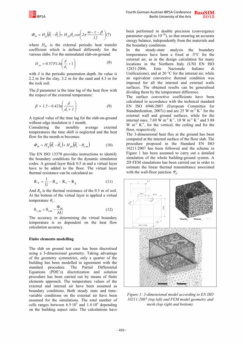
been performed in double precision (convergence parameter equal to 10-10), so that ensuring an accurate energy balance, independently from the materials and the boundary conditions. In the steady-state analysis the boundary temperatures have been a fixed at -5°C for the external air, as in the design calculation for many locations in the Northern Italy (UNI EN ISO 12831:2006, Ente Nazionale Italiano di Unificazione), and at 20 °C for the internal air, while an equivalent convective thermal condition was imposed for all the internal and external walls surfaces. The obtained results can be generalised dividing them by the temperature difference. The surface convective coefficients have been calculated in accordance with the technical standard EN ISO 6946:2007 (European Committee for Standardization, 2007c) and are 25 W m-2 K-1 for the external wall and ground surfaces, while for the internal ones, 7.69 W m-2 K-1, 10 W m-2 K-1 and 5.88 W m-2 K-1, for the vertical, the ceiling and for the floor, respectively. The 3-dimensional heat flux at the ground has been computed at the internal surface of the floor slab. The procedure proposed in the Standard EN ISO 10211:2007 has been followed and the scheme in Figure 1 has been assumed to carry out a detailed simulation of the whole building-ground system. A 2D FEM simulations has been carried out in order to estimate the linear thermal transmittance associated with the wall-floor junction g.

Figure 1: 3-dimensional model according to EN ISO 10211:2007 (top left) and FEM model geometry and

mesh (top right and bottom).

cb

0.5 c 2.5 b

0.5

b

2.5

b

3 b

0.5 c + 2.5 b

2.5

b

- 433 -

BauSIM2012


Table 2 Size and dimensions of the building (EN ISO

10211:2007)

Dimensions Insulation (m)

0.00 0.05 0.10

4:4 b 10.40 10.50 10.60 c 10.40 10.50 10.60

3:4 b 9.06 9.16 9.26 c 11.94 12.04 12.14

2:4 b 14.54 14.64 14.74 c 7.47 7.57 7.67

1:4 b 5.40 5.50 5.60 c 20.40 20.50 20.60

The external size and dimensions of the building and ground volumes have been reported in table 2. The internal floor area is 100 m2 for all the configurations.

RESULTS Steady-state and finite elements modelling

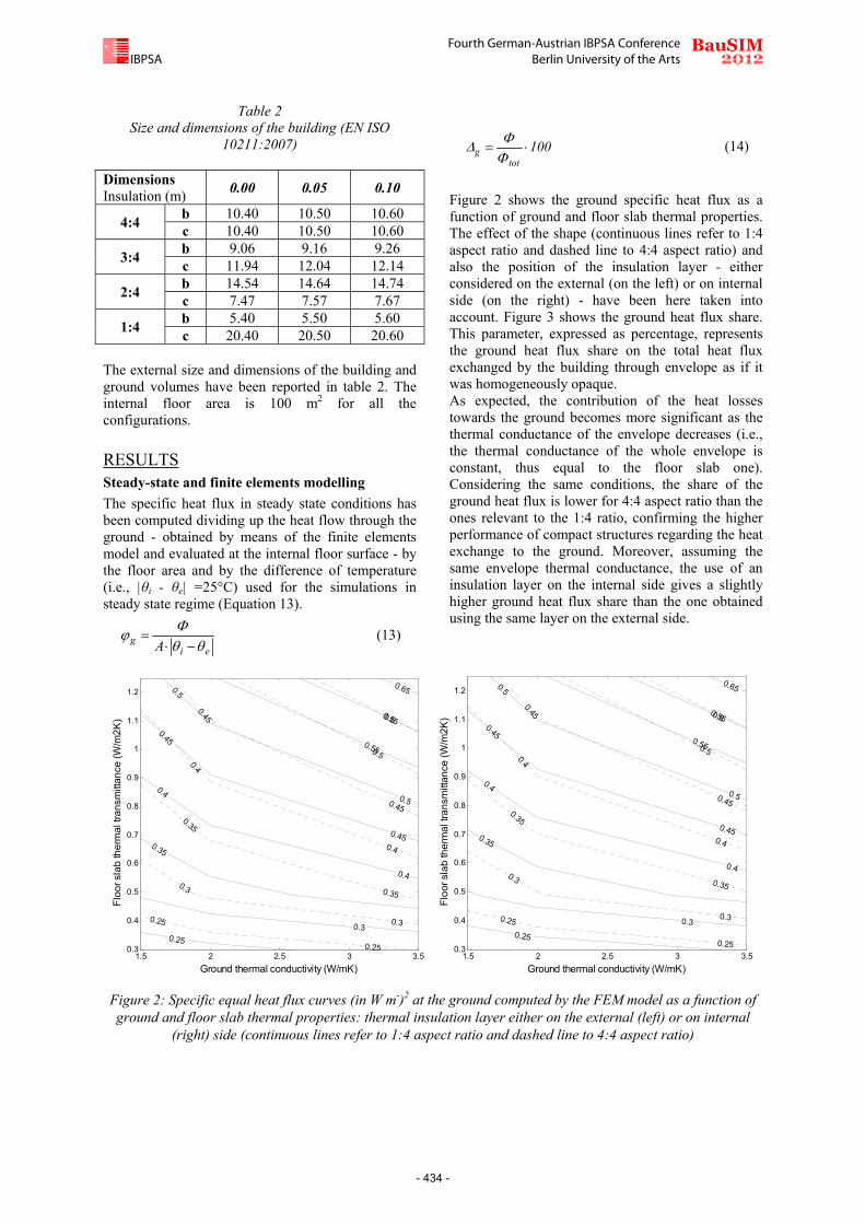
The specific heat flux in steady state conditions has been computed dividing up the heat flow through the ground - obtained by means of the finite elements model and evaluated at the internal floor surface - by the floor area and by the difference of temperature (i.e., |θi - θe| =25°C) used for the simulations in steady state regime (Equation 13).

eig A

(13)

100tot

g

(14)

Figure 2 shows the ground specific heat flux as a function of ground and floor slab thermal properties. The effect of the shape (continuous lines refer to 1:4 aspect ratio and dashed line to 4:4 aspect ratio) and also the position of the insulation layer - either considered on the external (on the left) or on internal side (on the right) - have been here taken into account. Figure 3 shows the ground heat flux share. This parameter, expressed as percentage, represents the ground heat flux share on the total heat flux exchanged by the building through envelope as if it was homogeneously opaque. As expected, the contribution of the heat losses towards the ground becomes more significant as the thermal conductance of the envelope decreases (i.e., the thermal conductance of the whole envelope is constant, thus equal to the floor slab one). Considering the same conditions, the share of the ground heat flux is lower for 4:4 aspect ratio than the ones relevant to the 1:4 ratio, confirming the higher performance of compact structures regarding the heat exchange to the ground. Moreover, assuming the same envelope thermal conductance, the use of an insulation layer on the internal side gives a slightly higher ground heat flux share than the one obtained using the same layer on the external side.

Figure 2: Specific equal heat flux curves (in W m-)2 at the ground computed by the FEM model as a function of ground and floor slab thermal properties: thermal insulation layer either on the external (left) or on internal

(right) side (continuous lines refer to 1:4 aspect ratio and dashed line to 4:4 aspect ratio)

0.25

0.3

0.35

0.4

0.4

0.45

0.45

0.5

0.5

0.55

0.6

0.65

Ground thermal conductivity (W/mK)

Flo

or s

lab

the

rmal

tra

nsm

ittan

ce (W

/m2

K)

0.25

0.25

0.3

0.3

0.35

0.35

0.4

0.4

0.45

0.45

0.5

0.55

1.5 2 2.5 3 3.50.3

0.4

0.5

0.6

0.7

0.8

0.9

1

1.1

1.2

0.25

0.3

0.35

0.4

0.4

0.45

0.45

0.5

0.5

0.55

0.6

0.65


Flo

or

sla

b th

erm

al t

ran

smitt

an

ce (

W/m

2K

)

0.25

0.25

0.3

0.3

0.35

0.35

0.4

0.4

0.45

0.45

0.5

0.55

1.5 2 2.5 3 3.50.3

0.4

0.5

0.6

0.7

0.8

0.9

1

1.1

1.2

- 434 -

BauSIM2012


Figure 3: Ground heat flux share curves (in %) computed by the FEM model as a function of ground and floor

slab thermal properties: thermal insulation layer either on the external (left) or on internal (right) side (continuous lines refer to 1:4 aspect ratio and dashed line to 4:4 aspect ratio)

Figure 4: Absolute percent deviations between the specific heat flux at the ground computed by means of the finite elements model (daily regime) and by means of the EN ISO 13370 procedure as a function of floor slab

thermal conductance, aspect ratios (on the left) or ground type (on the right). Dashed lines represent the envelope curves relevant either to the maximum or the minimum values for the limit aspect ratios (4:4 and 1:4).

The specific heat flux computed by means of the FEM model is here considered has a benchmark for the assessment of the performance of the EN ISO 13370:2007 standard procedure. An assessment of the deviations between the specific heat flux at the ground - computed by means of the finite elements model - and the one calculated by means of the EN ISO 13370:2007 standard procedure has been carried out. Figure 4 shows the computed deviations (as absolute values) as a function of floor slab thermal conductance and either aspect ratios (on the top) or ground type (on the bottom). Dashed lines represent the envelope curves relevant to the maximum and the minimum value for the limit aspect ratios (4:4 and 1:4 respectively). As a whole, the computed deviations are characterised by small values, always

lower than 1%, with a decreasing trend as the floor slab thermal conductance decreases. Regarding the shape of the building (Figure 4, left), the higher the slab thermal conductance values, the higher the differences between buildings with low and high aspect ratios. Buildings structures with 4:4 ratio are subjected to higher errors when using the standard procedure, resulting in values up to 0.98%.

The variation in the thermal properties of the ground (i.e., varying the kind of soil) also affects the performance of the standard computation if compared with the FEM modelling results (Figure 4, right). In particular, the maximum deviations have been detected for the rocky and sandy grounds, which are characterised by the higher thermal

1617

18

19

19 20

20

21

21

22

22

23

24


Flo

or

sla

b th

erm

al t

ran

smitt

an

ce (W

/m2

K)

1617

18

19

1920

20

21

21

22

22

23

23

24

24

25

26

1.5 2 2.5 3 3.50.3

0.4

0.5

0.6

0.7

0.8

0.9

1

1.1

1.2

1617

18

19

20

20

21

21

22

22

23

24

25


Flo

or

sla

b th

erm

al t

ran

smitt

anc

e (

W/m

2K

)

1617

18

19

19

20

20

21

21

22

22

23

23

24

24

25

26

1.5 2 2.5 3 3.50.3

0.4

0.5

0.6

0.7

0.8

0.9

1

1.1

1.2

0

0.2

0.4

0.6

0.8

1

0.0 0.5 1.0 1.5

Dev

iati

on

on

th

e s

pec

ific

hea

t fl

ux

(%

)

Floor slab thermal conductance (W m-2K-1)

(4:4) aspect ratio

(3:4) aspect ratio

(2:4) aspect ratio

(1:4) aspect ratio

max

min0.0

0.2

0.4

0.6

0.8

1.0

0.0 0.5 1.0 1.5

De

via

tio

n o

n t

he

sp

ec

ific

he

at

flu

x (

%)

Floor slab thermal conductance (W m-2K-1)

clay

sand

rock

- 435 -

BauSIM2012


conductivities. On the contrary, the values of the deviations relevant to the clay soil - which is characterised by the lowest thermal conductivity - are generally lower.

Periodic sinusoidal daily regime

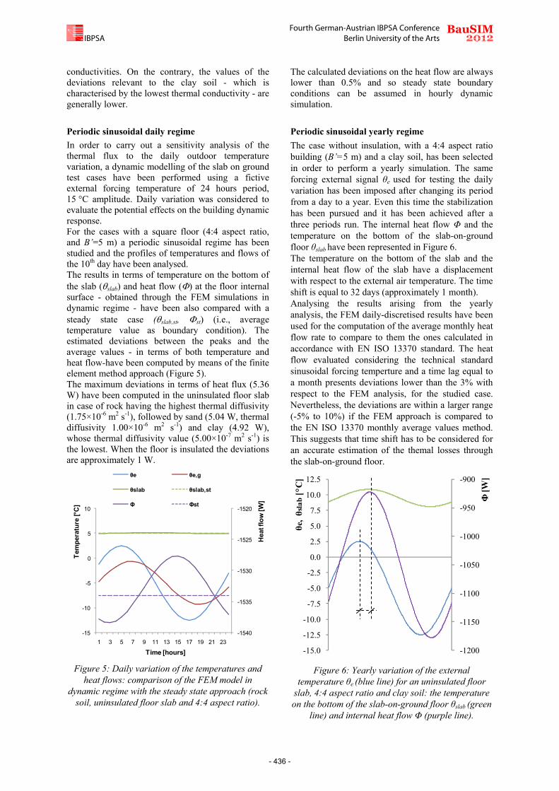
In order to carry out a sensitivity analysis of the thermal flux to the daily outdoor temperature variation, a dynamic modelling of the slab on ground test cases have been performed using a fictive external forcing temperature of 24 hours period, 15 °C amplitude. Daily variation was considered to evaluate the potential effects on the building dynamic response. For the cases with a square floor (4:4 aspect ratio, and B’=5 m) a periodic sinusoidal regime has been studied and the profiles of temperatures and flows of the 10th day have been analysed. The results in terms of temperature on the bottom of the slab (slab) and heat flow () at the floor internal surface - obtained through the FEM simulations in dynamic regime - have been also compared with a steady state case (slab,st, st) (i.e., average temperature value as boundary condition). The estimated deviations between the peaks and the average values - in terms of both temperature and heat flow-have been computed by means of the finite element method approach (Figure 5). The maximum deviations in terms of heat flux (5.36 W) have been computed in the uninsulated floor slab in case of rock having the highest thermal diffusivity (1.75×10-6 m2 s-1), followed by sand (5.04 W, thermal diffusivity 1.00×10-6 m2 s-1) and clay (4.92 W), whose thermal diffusivity value (5.00×10-7 m2 s-1) is the lowest. When the floor is insulated the deviations are approximately 1 W.

Figure 5: Daily variation of the temperatures and heat flows: comparison of the FEM model in

dynamic regime with the steady state approach (rock soil, uninsulated floor slab and 4:4 aspect ratio).

The calculated deviations on the heat flow are always lower than 0.5% and so steady state boundary conditions can be assumed in hourly dynamic simulation.

Periodic sinusoidal yearly regime

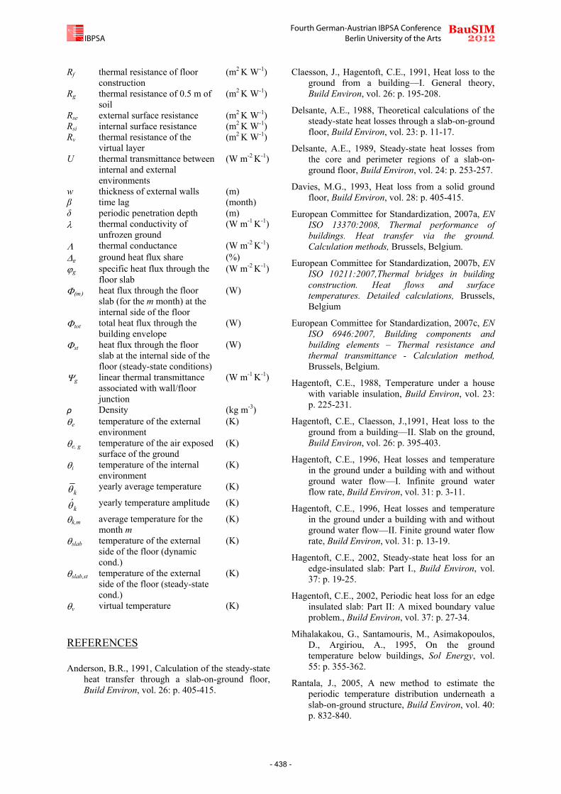
The case without insulation, with a 4:4 aspect ratio building (B’=5 m) and a clay soil, has been selected in order to perform a yearly simulation. The same forcing external signal θe

used for testing the daily variation has been imposed after changing its period from a day to a year. Even this time the stabilization has been pursued and it has been achieved after a three periods run. The internal heat flow Φ and the temperature on the bottom of the slab-on-ground floor θslab

have been represented in Figure 6. The temperature on the bottom of the slab and the internal heat flow of the slab have a displacement with respect to the external air temperature. The time shift is equal to 32 days (approximately 1 month). Analysing the results arising from the yearly analysis, the FEM daily-discretised results have been used for the computation of the average monthly heat flow rate to compare to them the ones calculated in accordance with EN ISO 13370 standard. The heat flow evaluated considering the technical standard sinusoidal forcing temperture and a time lag equal to a month presents deviations lower than the 3% with respect to the FEM analysis, for the studied case. Nevertheless, the deviations are within a larger range (-5% to 10%) if the FEM approach is compared to the EN ISO 13370 monthly average values method. This suggests that time shift has to be considered for an accurate estimation of the themal losses through the slab-on-ground floor.

Figure 6: Yearly variation of the external temperature θe

(blue line) for an uninsulated floor slab, 4:4 aspect ratio and clay soil: the temperature on the bottom of the slab-on-ground floor θslab

(green line) and internal heat flow Φ (purple line).

-1540

-1535

-1530

-1525

-1520

-15

-10

-5

0

5

10

1 3 5 7 9 11 13 15 17 19 21 23

Hea

t flo

w [W

]

Tem

per

atu

re [°

C]

Time [hours]

θe θe,g

θslab θslab,st

Φ Φst

-1200

-1150

-1100

-1050

-1000

-950

-900

-15.0

-12.5

-10.0

-7.5

-5.0

-2.5

0.0

2.5

5.0

7.5

10.0

12.5Φ

[W]

θ e, θs

lab

[°C

]

- 436 -

BauSIM2012


Analysing the results arising from the yearly analysis, the FEM daily-discretised results have been used for the computation of the average monthly heat flow rate to compare to them the ones calculated in accordance with EN ISO 13370 standard. The heat flow evaluated considering the technical standard sinusoidal forcing temperture and a time lag equal to a month presents deviations lower than the 3% with respect to the FEM analysis, for the studied case. Nevertheless, the deviations are within a larger range (-5% to 10%) if the FEM approach is compared to the EN ISO 13370 monthly average values method. This suggests that time shift has to be considered for an accurate estimation of the themal losses through the slab-on-ground floor. The heat flow values have been used for the estimation of the monthly virtual temperatures in agreement with the technical standard procedure, as in Figure 7. The accuracy is again affected by the correct estimation of the time shift. Thus, the sinusoidal forcing temperature approach presents deviations lower than 1 °C on the temperatures while for the average monthly method the deviations are within a larger range of 2 °C.

Figure 7:Virtual temperatures calculated starting from different monthly heat flow rate (rock soil,

uninsulated floor slab and 4:4 aspect ratio).

CONCLUSIONS In this paper, the slab on ground floor and the methods proposed by the technical standard EN ISO 13370 have been assessed by means of a comparison with a finite elements methods (FEM) code. Different types of floor characterised by different thicknesses, positions of the insulation layer and shapes (aspect ratios) have been taken into account for this analysis. The specific heat flux and the share of the ground heat flux on the total heat flow through the whole building envelope, as it is was opaque, have been computed in steady state regime both using the detailed numerical approaches or the analytical ones proposed by the standard. The effect of the soil and floor slab thermal properties, the effect of the aspect ratio of the building has been considered for the

analysis. The more compact, the more efficient the building structure is. The use of an internal insulation layer also gives better performances in terms of specific heat flux, but not in terms of ground heat flux share on the total heat flux through the envelope. The comparison between the predictions of the technical standard and the FEM modelling results has been carried out through a detailed assessment of floor losses. Once again, compact building structure are the more efficient, as they are subjected to lower errors when using the standard procedure. The variation in the thermal properties of the ground also affects the performance of the standard procedure: the lower the soil thermal conductivity, the smaller the deviations between the standard and the FEM modelling. Moreover, a dynamic analysis has been carried out in order to assess the procedure proposed by the standard for determining the boundary conditions to be used in building simulation codes such as TRNSYS and EnergyPlus. First of all, a sinusoidal external boundary condition on temperature of one day period have been used to evaluate the deviations between the dynamic and the steady state modelling. The estimated deviations between the peaks and the average values - in terms of both temperature and heat flux computed by means of the FEM approach - resulted negligible (less than 0.1 °C for the temperature, less than the 0.5% for the heat flow). Therefore, steady-state boundary conditions on the ground side can be assumed also for the dynamic simulation when interesting in evaluating the thermal behaviour of a building with a hourly (or more detailed) discretization on periodical analysis. The dynamic of the heat transfer through the soil has to be consider on larger periods, so far with a yearly periodic condition. Two different approaches suggested by the technical standard for estimating the monthly heat flow have been considered and used for elaborating the virtual temperature to be used in dynamic simulation codes. It has been found that the time shift has to be taken into account in order to achieve lower errors (1 °C for the virtual temperature and less than 3% in the heat flow rate estimation).

NOMENCLATURE

A area of floor (m2) B´ characteristic dimension of

floor (m)

c specific heat capacity (J kg-1K-1) dt total equivalent thickness -

slab on ground floor (m)

Hg steady-state ground heat transfer coefficient

(W K-1)

Hpe external periodic heat transfer coefficient

(W K-1)

P exposed perimeter of floor (m)

-12

-10

-8

-6

-4

-2

-

1 2 3 4 5 6 7 8 9 10 11 12

Vir

tual T

em

pe

ratu

re θ

v[°

C]

Month

FEM

EN ISO 13370: sinusoidal forcing temperature

EN ISO 13370: average monthly temperatures

- 437 -

BauSIM2012


Rf thermal resistance of floor construction

(m2 K W-1)

Rg thermal resistance of 0.5 m of soil

(m2 K W-1)

Rse external surface resistance (m2 K W-1) Rsi internal surface resistance (m2 K W-1) Rv thermal resistance of the

virtual layer (m2 K W-1)

U thermal transmittance between internal and external environments

(W m-2 K-1)

w thickness of external walls (m) β time lag (month) δ periodic penetration depth (m) thermal conductivity of

unfrozen ground (W m-1 K-1)

thermal conductance (W m-2 K-1) g ground heat flux share (%) g specific heat flux through the

floor slab (W m-2 K-1)

m heat flux through the floor slab (for the m month) at the internal side of the floor

(W)

tot total heat flux through the building envelope

(W)

st heat flux through the floor slab at the internal side of the floor (steady-state conditions)

(W)

g linear thermal transmittance associated with wall/floor junction

(W m-1 K-1)

ρ Density (kg m-3) e temperature of the external

environment (K)

e, g temperature of the air exposed surface of the ground

(K)

i temperature of the internal environment

(K)

k yearly average temperature (K)

k̂ yearly temperature amplitude (K)

k,m average temperature for the month m

(K)

slab temperature of the external side of the floor (dynamic cond.)

(K)

slab,st temperature of the external side of the floor (steady-state cond.)

(K)

v virtual temperature (K)

REFERENCES Anderson, B.R., 1991, Calculation of the steady-state

heat transfer through a slab-on-ground floor, Build Environ, vol. 26: p. 405-415.

Claesson, J., Hagentoft, C.E., 1991, Heat loss to the ground from a building—I. General theory, Build Environ, vol. 26: p. 195-208.

Delsante, A.E., 1988, Theoretical calculations of the steady-state heat losses through a slab-on-ground floor, Build Environ, vol. 23: p. 11-17.

Delsante, A.E., 1989, Steady-state heat losses from the core and perimeter regions of a slab-on-ground floor, Build Environ, vol. 24: p. 253-257.

Davies, M.G., 1993, Heat loss from a solid ground floor, Build Environ, vol. 28: p. 405-415.

European Committee for Standardization, 2007a, EN ISO 13370:2008, Thermal performance of buildings. Heat transfer via the ground. Calculation methods, Brussels, Belgium.

European Committee for Standardization, 2007b, EN ISO 10211:2007,Thermal bridges in building construction. Heat flows and surface temperatures. Detailed calculations, Brussels, Belgium

European Committee for Standardization, 2007c, EN ISO 6946:2007, Building components and building elements – Thermal resistance and thermal transmittance - Calculation method, Brussels, Belgium.

Hagentoft, C.E., 1988, Temperature under a house with variable insulation, Build Environ, vol. 23: p. 225-231.

Hagentoft, C.E., Claesson, J.,1991, Heat loss to the ground from a building—II. Slab on the ground, Build Environ, vol. 26: p. 395-403.

Hagentoft, C.E., 1996, Heat losses and temperature in the ground under a building with and without ground water flow—I. Infinite ground water flow rate, Build Environ, vol. 31: p. 3-11.

Hagentoft, C.E., 1996, Heat losses and temperature in the ground under a building with and without ground water flow—II. Finite ground water flow rate, Build Environ, vol. 31: p. 13-19.

Hagentoft, C.E., 2002, Steady-state heat loss for an edge-insulated slab: Part I., Build Environ, vol. 37: p. 19-25.

Hagentoft, C.E., 2002, Periodic heat loss for an edge insulated slab: Part II: A mixed boundary value problem., Build Environ, vol. 37: p. 27-34.

Mihalakakou, G., Santamouris, M., Asimakopoulos, D., Argiriou, A., 1995, On the ground temperature below buildings, Sol Energy, vol. 55: p. 355-362.

Rantala, J., 2005, A new method to estimate the periodic temperature distribution underneath a slab-on-ground structure, Build Environ, vol. 40: p. 832-840.

- 438 -

Documents

Fourth German-Austrian IBPSA ConferenceBauSIM IBPSA Berlin ... · Fourth German-Austrian IBPSA Conference IBPSA Berlin University of the Arts 3D UNSTEADY STATE ANALYSIS OF THERMAL