Fourier transform

From Wikipedia, the free encyclopedia

Jump to: navigation, search

The Fourier transform is a mathematical operation that decomposes a signal into its

constituent frequencies. Thus the Fourier transform of a musical chord is a mathematical

representation of the amplitudes of the individual notes that make it up. The original

signal depends on time, and therefore is called the time domain representation of the

signal, whereas the Fourier transform depends on frequency and is called the frequency

domain representation of the signal. The term Fourier transform refers both to the

frequency domain representation of the signal and the process that transforms the signal

to its frequency domain representation.

In mathematical terms, the Fourier transform 'transforms' one complex-valued function of

a real variable into another. In effect, the Fourier transform decomposes a function into

oscillatory functions. The Fourier transform and its generalizations are the subject of

Fourier analysis. In this specific case, both the time and frequency domains are

unbounded linear continua. It is possible to define the Fourier transform of a function of

several variables, which is important for instance in the physical study of wave motion

and optics. It is also possible to generalize the Fourier transform on discrete structures

such as finite groups. The efficient computation of such structures, by fast Fourier

transform, is essential for high-speed computing.

Fourier transforms

Continuous Fourier transform

Fourier series

Discrete Fourier transform

Discrete-time Fourier transform

Related transforms

Contents

1 Definition

2 Introduction

3 Properties of the Fourier transform

o 3.1 Basic properties

o 3.2 Uniform continuity and the Riemann–Lebesgue lemma

o 3.3 The Plancherel theorem and Parseval's theorem

o 3.4 Poisson summation formula

o 3.5 Convolution theorem

o 3.6 Cross-correlation theorem

o 3.7 Eigenfunctions

4 Fourier transform on Euclidean space

o 4.1 Uncertainty principle

o 4.2 Spherical harmonics

o 4.3 Restriction problems

5 Generalizations

o 5.1 Fourier transform on other function spaces

o 5.2 Fourier–Stieltjes transform

o 5.3 Tempered distributions

o 5.4 Locally compact abelian groups

o 5.5 Locally compact Hausdorff space

o 5.6 Non-abelian groups

6 Alternatives

7 Applications

o 7.1 Analysis of differential equations

o 7.2 Fourier transform spectroscopy

8 Domain and range of the Fourier transform

9 Other notations

10 Other conventions

11 Tables of important Fourier transforms

o 11.1 Functional relationships

o 11.2 Square-integrable functions

o 11.3 Distributions

o 11.4 Two-dimensional functions

o 11.5 Formulas for general n-dimensional functions

12 See also

13 References

14 External links

[edit] Definition

There are several common conventions for defining the Fourier transform of an

integrable function ƒ : R → C (Kaiser 1994). This article will use the definition:

for every real number ξ.

When the independent variable x represents time (with SI unit of seconds), the transform

variable ξ represents frequency (in hertz). Under suitable conditions, ƒ can be

reconstructed from by the inverse transform:

for every real number x.

For other common conventions and notations, including using the angular frequency ω

instead of the frequency ξ, see Other conventions and Other notations below. The Fourier

transform on Euclidean space is treated separately, in which the variable x often

represents position and ξ momentum.

[edit] Introduction

See also: Fourier analysis

The motivation for the Fourier transform comes from the study of Fourier series. In the

study of Fourier series, complicated functions are written as the sum of simple waves

mathematically represented by sines and cosines. Due to the properties of sine and cosine

it is possible to recover the amount of each wave in the sum by an integral. In many cases

it is desirable to use Euler's formula, which states that e2πiθ

= cos 2πθ + i sin 2πθ, to write

Fourier series in terms of the basic waves e2πiθ

. This has the advantage of simplifying

many of the formulas involved and providing a formulation for Fourier series that more

closely resembles the definition followed in this article. This passage from sines and

cosines to complex exponentials makes it necessary for the Fourier coefficients to be

complex valued. The usual interpretation of this complex number is that it gives both the

amplitude (or size) of the wave present in the function and the phase (or the initial angle)

of the wave. This passage also introduces the need for negative "frequencies". If θ were

measured in seconds then the waves e2πiθ

and e−2πiθ

would both complete one cycle per

second, but they represent different frequencies in the Fourier transform. Hence,

frequency no longer measures the number of cycles per unit time, but is closely related.

There is a close connection between the definition of Fourier series and the Fourier

transform for functions ƒ which are zero outside of an interval. For such a function we

can calculate its Fourier series on any interval that includes the interval where ƒ is not

identically zero. The Fourier transform is also defined for such a function. As we increase

the length of the interval on which we calculate the Fourier series, then the Fourier series

coefficients begin to look like the Fourier transform and the sum of the Fourier series of ƒ

begins to look like the inverse Fourier transform. To explain this more precisely, suppose

that T is large enough so that the interval [−T/2,T/2] contains the interval on which ƒ is

not identically zero. Then the n-th series coefficient cn is given by:

Comparing this to the definition of the Fourier transform it follows that

since ƒ(x) is zero outside [−T/2,T/2]. Thus the Fourier coefficients are just the values of

the Fourier transform sampled on a grid of width 1/T. As T increases the Fourier

coefficients more closely represent the Fourier transform of the function.

Under appropriate conditions the sum of the Fourier series of ƒ will equal the function ƒ.

In other words ƒ can be written:

where the last sum is simply the first sum rewritten using the definitions ξn = n/T, and

Δξ = (n + 1)/T − n/T = 1/T.

This second sum is a Riemann sum, and so by letting T → ∞ it will converge to the

integral for the inverse Fourier transform given in the definition section. Under suitable

conditions this argument may be made precise (Stein & Shakarchi 2003).

In the study of Fourier series the numbers cn could be thought of as the "amount" of the

wave in the Fourier series of ƒ. Similarly, as seen above, the Fourier transform can be

thought of as a function that measures how much of each individual frequency is present

in our function ƒ, and we can recombine these waves by using an integral (or "continuous

sum") to reproduce the original function.

The following images provide a visual illustration of how the Fourier transform measures

whether a frequency is present in a particular function. The function depicted

oscillates at 3 hertz (if t measures seconds) and tends quickly to

0. This function was specially chosen to have a real Fourier transform which can easily

be plotted. The first image contains its graph. In order to calculate we must

integrate e−2πi(3t)

ƒ(t). The second image shows the plot of the real and imaginary parts of

this function. The real part of the integrand is almost always positive, this is because

when ƒ(t) is negative, then the real part of e−2πi(3t)

is negative as well. Because they

oscillate at the same rate, when ƒ(t) is positive, so is the real part of e−2πi(3t)

. The result is

that when you integrate the real part of the integrand you get a relatively large number (in

this case 0.5). On the other hand, when you try to measure a frequency that is not present,

as in the case when we look at , the integrand oscillates enough so that the integral

is very small. The general situation may be a bit more complicated than this, but this in

spirit is how the Fourier transform measures how much of an individual frequency is

present in a function ƒ(t).

Original function showing oscillation 3 hertz.

Real and imaginary parts of integrand for Fourier transform at 3 hertz

Real and imaginary parts of integrand for Fourier transform at 5 hertz

Fourier transform with 3 and 5 hertz labeled.

[edit] Properties of the Fourier transform

An integrable function is a function ƒ on the real line that is Lebesgue-measurable and

satisfies

[edit] Basic properties

Given integrable functions f(x), g(x), and h(x) denote their Fourier transforms by ,

, and respectively. The Fourier transform has the following basic properties

(Pinsky 2002).

Linearity

For any complex numbers a and b, if h(x) = aƒ(x) + bg(x), then 

Translation

For any real number x0, if h(x) = ƒ(x − x0), then 

Modulation

For any real number ξ0, if h(x) = e2πixξ

0ƒ(x), then  .

Scaling

For a non-zero real number a, if h(x) = ƒ(ax), then  . The

case a = −1 leads to the time-reversal property, which states: if h(x) = ƒ(−x), then 

.

Conjugation

If , then 

In particular, if ƒ is real, then one has the reality condition 

And if ƒ is purely imaginary, then 

Duality

If then 

Convolution

If , then 

[edit] Uniform continuity and the Riemann–Lebesgue lemma

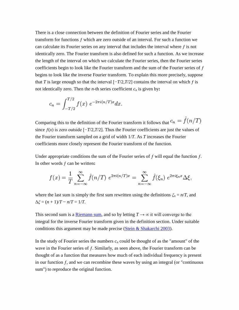
The rectangular function is Lebesgue integrable.

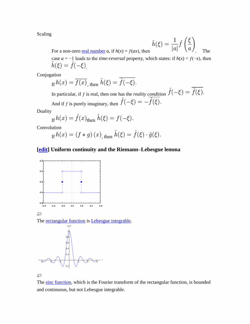
The sinc function, which is the Fourier transform of the rectangular function, is bounded

and continuous, but not Lebesgue integrable.

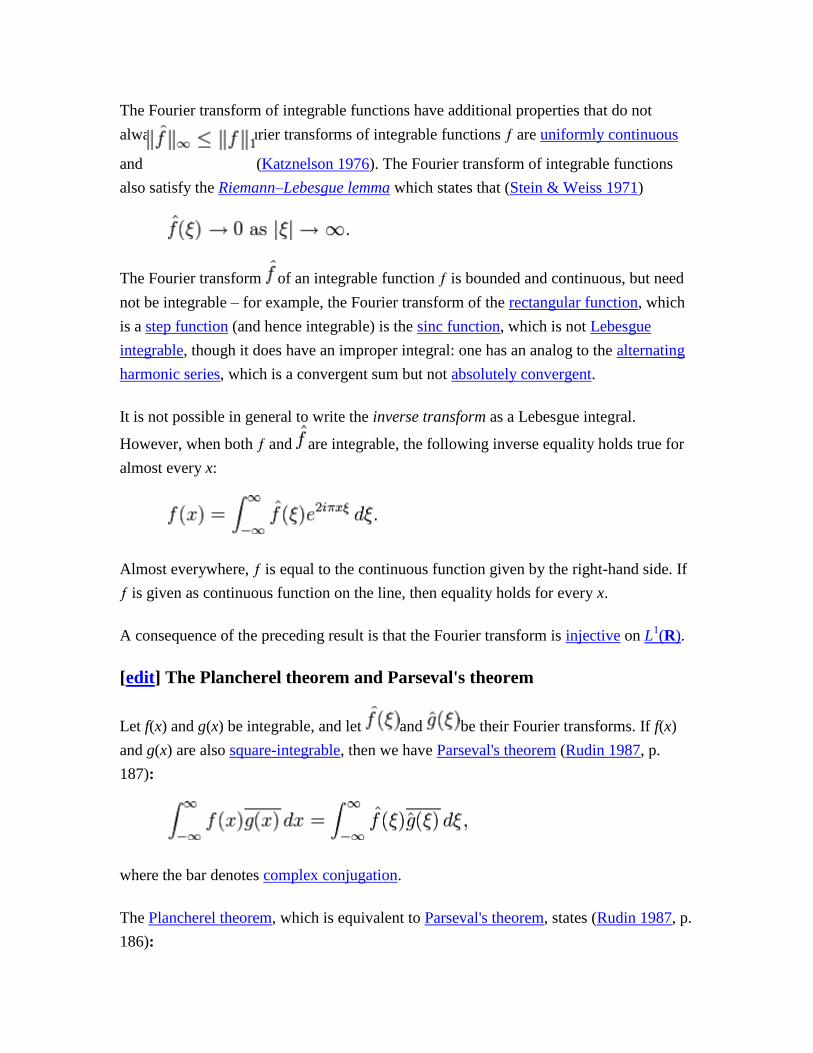
The Fourier transform of integrable functions have additional properties that do not

always hold. The Fourier transforms of integrable functions ƒ are uniformly continuous

and (Katznelson 1976). The Fourier transform of integrable functions

also satisfy the Riemann–Lebesgue lemma which states that (Stein & Weiss 1971)

The Fourier transform of an integrable function ƒ is bounded and continuous, but need

not be integrable – for example, the Fourier transform of the rectangular function, which

is a step function (and hence integrable) is the sinc function, which is not Lebesgue

integrable, though it does have an improper integral: one has an analog to the alternating

harmonic series, which is a convergent sum but not absolutely convergent.

It is not possible in general to write the inverse transform as a Lebesgue integral.

However, when both ƒ and are integrable, the following inverse equality holds true for

almost every x:

Almost everywhere, ƒ is equal to the continuous function given by the right-hand side. If

ƒ is given as continuous function on the line, then equality holds for every x.

A consequence of the preceding result is that the Fourier transform is injective on L1(R).

[edit] The Plancherel theorem and Parseval's theorem

Let f(x) and g(x) be integrable, and let and be their Fourier transforms. If f(x)

and g(x) are also square-integrable, then we have Parseval's theorem (Rudin 1987, p.

187):

where the bar denotes complex conjugation.

The Plancherel theorem, which is equivalent to Parseval's theorem, states (Rudin 1987, p.

186):

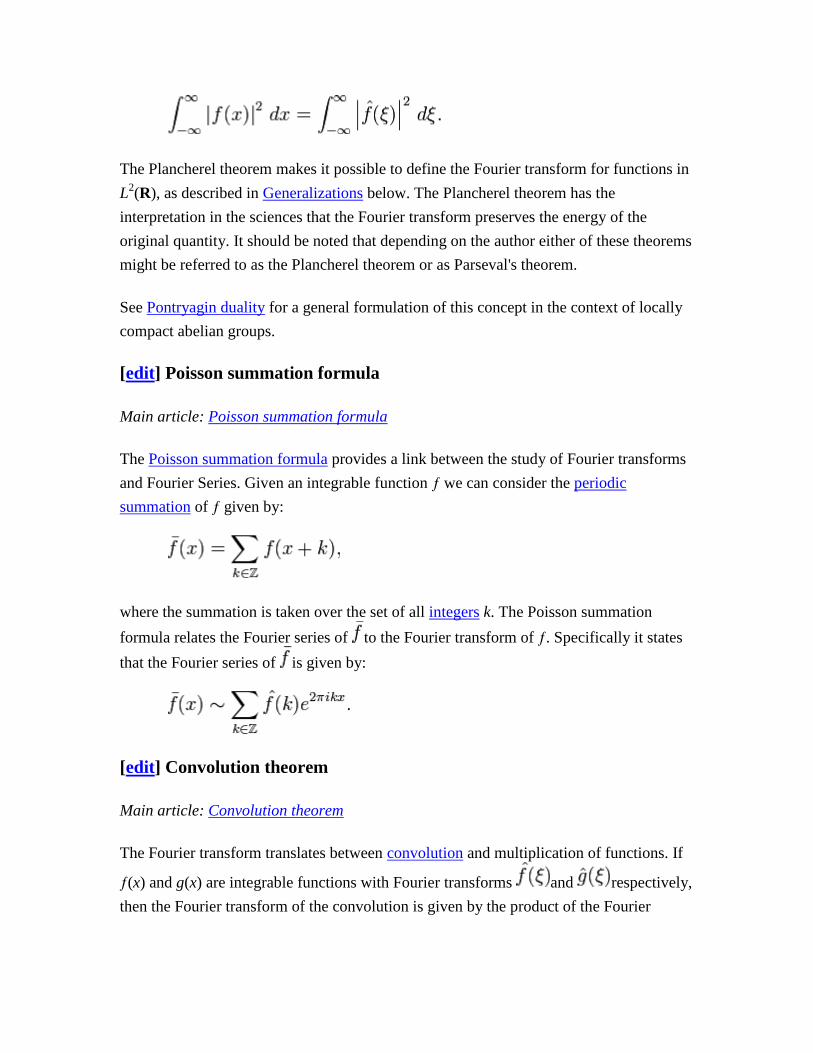
The Plancherel theorem makes it possible to define the Fourier transform for functions in

L2(R), as described in Generalizations below. The Plancherel theorem has the

interpretation in the sciences that the Fourier transform preserves the energy of the

original quantity. It should be noted that depending on the author either of these theorems

might be referred to as the Plancherel theorem or as Parseval's theorem.

See Pontryagin duality for a general formulation of this concept in the context of locally

compact abelian groups.

[edit] Poisson summation formula

Main article: Poisson summation formula

The Poisson summation formula provides a link between the study of Fourier transforms

and Fourier Series. Given an integrable function ƒ we can consider the periodic

summation of ƒ given by:

where the summation is taken over the set of all integers k. The Poisson summation

formula relates the Fourier series of to the Fourier transform of ƒ. Specifically it states

that the Fourier series of is given by:

[edit] Convolution theorem

Main article: Convolution theorem

The Fourier transform translates between convolution and multiplication of functions. If

ƒ(x) and g(x) are integrable functions with Fourier transforms and respectively,

then the Fourier transform of the convolution is given by the product of the Fourier

transforms and (under other conventions for the definition of the Fourier

transform a constant factor may appear).

This means that if:

where ∗ denotes the convolution operation, then:

In linear time invariant (LTI) system theory, it is common to interpret g(x) as the impulse

response of an LTI system with input ƒ(x) and output h(x), since substituting the unit

impulse for ƒ(x) yields h(x) = g(x). In this case,    represents the frequency response

of the system.

Conversely, if ƒ(x) can be decomposed as the product of two square integrable functions

p(x) and q(x), then the Fourier transform of ƒ(x) is given by the convolution of the

respective Fourier transforms and .

[edit] Cross-correlation theorem

Main article: Cross-correlation

In an analogous manner, it can be shown that if h(x) is the cross-correlation of ƒ(x) and

g(x):

then the Fourier transform of h(x) is:

As a special case, the autocorrelation of function ƒ(x) is:

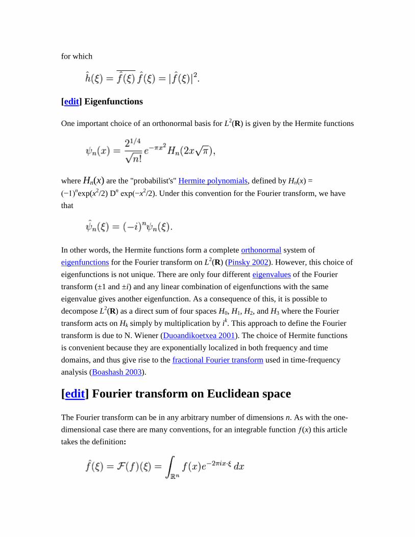
for which

[edit] Eigenfunctions

One important choice of an orthonormal basis for L2(R) is given by the Hermite functions

where Hn(x) are the "probabilist's" Hermite polynomials, defined by Hn(x) =

(−1)nexp(x

2/2) D

n exp(−x

2/2). Under this convention for the Fourier transform, we have

that

In other words, the Hermite functions form a complete orthonormal system of

eigenfunctions for the Fourier transform on L2(R) (Pinsky 2002). However, this choice of

eigenfunctions is not unique. There are only four different eigenvalues of the Fourier

transform (±1 and ±i) and any linear combination of eigenfunctions with the same

eigenvalue gives another eigenfunction. As a consequence of this, it is possible to

decompose L2(R) as a direct sum of four spaces H0, H1, H2, and H3 where the Fourier

transform acts on Hk simply by multiplication by ik. This approach to define the Fourier

transform is due to N. Wiener (Duoandikoetxea 2001). The choice of Hermite functions

is convenient because they are exponentially localized in both frequency and time

domains, and thus give rise to the fractional Fourier transform used in time-frequency

analysis (Boashash 2003).

[edit] Fourier transform on Euclidean space

The Fourier transform can be in any arbitrary number of dimensions n. As with the one-

dimensional case there are many conventions, for an integrable function ƒ(x) this article

takes the definition:

where x and ξ are n-dimensional vectors, and x · ξ is the dot product of the vectors. The

dot product is sometimes written as .

All of the basic properties listed above hold for the n-dimensional Fourier transform, as

do Plancherel's and Parseval's theorem. When the function is integrable, the Fourier

transform is still uniformly continuous and the Riemann–Lebesgue lemma holds. (Stein

& Weiss 1971)

[edit] Uncertainty principle

Generally speaking, the more concentrated f(x) is, the more spread out its Fourier

transform   must be. In particular, the scaling property of the Fourier transform may

be seen as saying: if we "squeeze" a function in x, its Fourier transform "stretches out" in

ξ. It is not possible to arbitrarily concentrate both a function and its Fourier transform.

The trade-off between the compaction of a function and its Fourier transform can be

formalized in the form of an Uncertainty Principle by viewing a function and its Fourier

transform as conjugate variables with respect to the symplectic form on the time–

frequency domain: from the point of view of the linear canonical transformation, the

Fourier transform is rotation by 90° in the time–frequency domain, and preserves the

symplectic form.

Suppose ƒ(x) is an integrable and square-integrable function. Without loss of generality,

assume that ƒ(x) is normalized:

It follows from the Plancherel theorem that   is also normalized.

The spread around x = 0 may be measured by the dispersion about zero (Pinsky 2002)

defined by

In probability terms, this is the second moment of about zero.

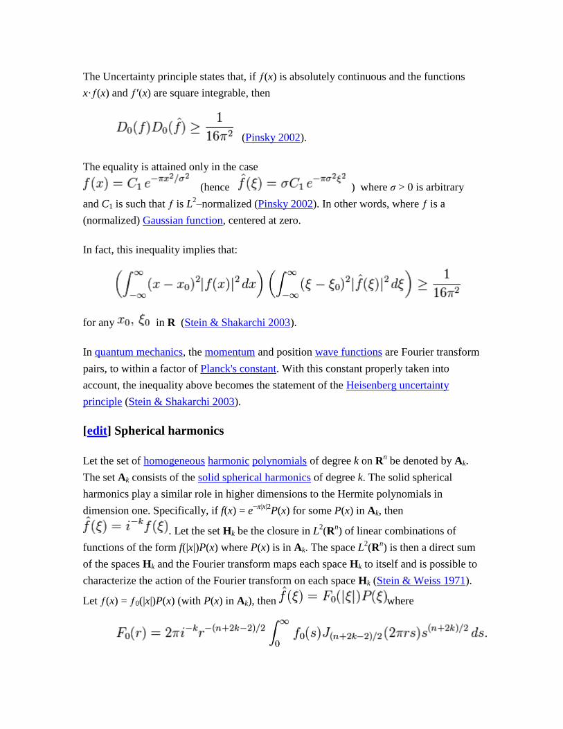
The Uncertainty principle states that, if ƒ(x) is absolutely continuous and the functions

x·ƒ(x) and ƒ′(x) are square integrable, then

(Pinsky 2002).

The equality is attained only in the case

(hence ) where σ > 0 is arbitrary

and C1 is such that ƒ is L2–normalized (Pinsky 2002). In other words, where ƒ is a

(normalized) Gaussian function, centered at zero.

In fact, this inequality implies that:

for any in R (Stein & Shakarchi 2003).

In quantum mechanics, the momentum and position wave functions are Fourier transform

pairs, to within a factor of Planck's constant. With this constant properly taken into

account, the inequality above becomes the statement of the Heisenberg uncertainty

principle (Stein & Shakarchi 2003).

[edit] Spherical harmonics

Let the set of homogeneous harmonic polynomials of degree k on Rn be denoted by Ak.

The set Ak consists of the solid spherical harmonics of degree k. The solid spherical

harmonics play a similar role in higher dimensions to the Hermite polynomials in

dimension one. Specifically, if f(x) = e−π|x|2

P(x) for some P(x) in Ak, then

. Let the set Hk be the closure in L2(R

n) of linear combinations of

functions of the form f(|x|)P(x) where P(x) is in Ak. The space L2(R

n) is then a direct sum

of the spaces Hk and the Fourier transform maps each space Hk to itself and is possible to

characterize the action of the Fourier transform on each space Hk (Stein & Weiss 1971).

Let ƒ(x) = ƒ0(|x|)P(x) (with P(x) in Ak), then where

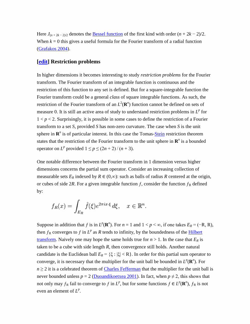
Here J(n + 2k − 2)/2 denotes the Bessel function of the first kind with order (n + 2k − 2)/2.

When k = 0 this gives a useful formula for the Fourier transform of a radial function

(Grafakos 2004).

[edit] Restriction problems

In higher dimensions it becomes interesting to study restriction problems for the Fourier

transform. The Fourier transform of an integrable function is continuous and the

restriction of this function to any set is defined. But for a square-integrable function the

Fourier transform could be a general class of square integrable functions. As such, the

restriction of the Fourier transform of an L2(R

n) function cannot be defined on sets of

measure 0. It is still an active area of study to understand restriction problems in Lp for

1 < p < 2. Surprisingly, it is possible in some cases to define the restriction of a Fourier

transform to a set S, provided S has non-zero curvature. The case when S is the unit

sphere in Rn is of particular interest. In this case the Tomas-Stein restriction theorem

states that the restriction of the Fourier transform to the unit sphere in Rn is a bounded

operator on Lp provided 1 ≤ p ≤ (2n + 2) / (n + 3).

One notable difference between the Fourier transform in 1 dimension versus higher

dimensions concerns the partial sum operator. Consider an increasing collection of

measurable sets ER indexed by R ∈ (0,∞): such as balls of radius R centered at the origin,

or cubes of side 2R. For a given integrable function ƒ, consider the function ƒR defined

by:

Suppose in addition that ƒ is in Lp(R

n). For n = 1 and 1 < p < ∞, if one takes ER = (−R, R),

then ƒR converges to ƒ in Lp as R tends to infinity, by the boundedness of the Hilbert

transform. Naively one may hope the same holds true for n > 1. In the case that ER is

taken to be a cube with side length R, then convergence still holds. Another natural

candidate is the Euclidean ball ER = {ξ : |ξ| < R}. In order for this partial sum operator to

converge, it is necessary that the multiplier for the unit ball be bounded in Lp(R

n). For

n ≥ 2 it is a celebrated theorem of Charles Fefferman that the multiplier for the unit ball is

never bounded unless p = 2 (Duoandikoetxea 2001). In fact, when p ≠ 2, this shows that

not only may ƒR fail to converge to ƒ in Lp, but for some functions ƒ ∈ L

p(R

n), ƒR is not

even an element of Lp.

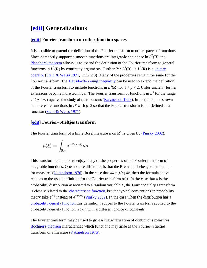
[edit] Generalizations

[edit] Fourier transform on other function spaces

It is possible to extend the definition of the Fourier transform to other spaces of functions.

Since compactly supported smooth functions are integrable and dense in L2(R), the

Plancherel theorem allows us to extend the definition of the Fourier transform to general

functions in L2(R) by continuity arguments. Further : L

2(R) → L

2(R) is a unitary

operator (Stein & Weiss 1971, Thm. 2.3). Many of the properties remain the same for the

Fourier transform. The Hausdorff–Young inequality can be used to extend the definition

of the Fourier transform to include functions in Lp(R) for 1 ≤ p ≤ 2. Unfortunately, further

extensions become more technical. The Fourier transform of functions in Lp for the range

2 < p < ∞ requires the study of distributions (Katznelson 1976). In fact, it can be shown

that there are functions in Lp with p>2 so that the Fourier transform is not defined as a

function (Stein & Weiss 1971).

[edit] Fourier–Stieltjes transform

The Fourier transform of a finite Borel measure μ on Rn is given by (Pinsky 2002):

This transform continues to enjoy many of the properties of the Fourier transform of

integrable functions. One notable difference is that the Riemann–Lebesgue lemma fails

for measures (Katznelson 1976). In the case that dμ = ƒ(x) dx, then the formula above

reduces to the usual definition for the Fourier transform of ƒ. In the case that μ is the

probability distribution associated to a random variable X, the Fourier-Stieltjes transform

is closely related to the characteristic function, but the typical conventions in probability

theory take eix·ξ

instead of e−2πix·ξ

(Pinsky 2002). In the case when the distribution has a

probability density function this definition reduces to the Fourier transform applied to the

probability density function, again with a different choice of constants.

The Fourier transform may be used to give a characterization of continuous measures.

Bochner's theorem characterizes which functions may arise as the Fourier–Stieltjes

transform of a measure (Katznelson 1976).

Furthermore, the Dirac delta function is not a function but it is a finite Borel measure. Its

Fourier transform is a constant function (whose specific value depends upon the form of

the Fourier transform used).

[edit] Tempered distributions

Main article: Tempered distributions

The Fourier transform maps the space of Schwartz functions to itself, and gives a

homeomorphism of the space to itself (Stein & Weiss 1971). Because of this it is possible

to define the Fourier transform of tempered distributions. These include all the integrable

functions mentioned above, as well as well-behaved functions of polynomial growth and

distributions of compact support, and have the added advantage that the Fourier

transform of any tempered distribution is again a tempered distribution.

The following two facts provide some motivation for the definition of the Fourier

transform of a distribution. First let ƒ and g be integrable functions, and let and be

their Fourier transforms respectively. Then the Fourier transform obeys the following

multiplication formula (Stein & Weiss 1971),

Secondly, every integrable function ƒ defines a distribution Tƒ by the relation

for all Schwartz functions φ.

In fact, given a distribution T, we define the Fourier transform by the relation

for all Schwartz functions φ.

It follows that

Distributions can be differentiated and the above mentioned compatibility of the Fourier

transform with differentiation and convolution remains true for tempered distributions.

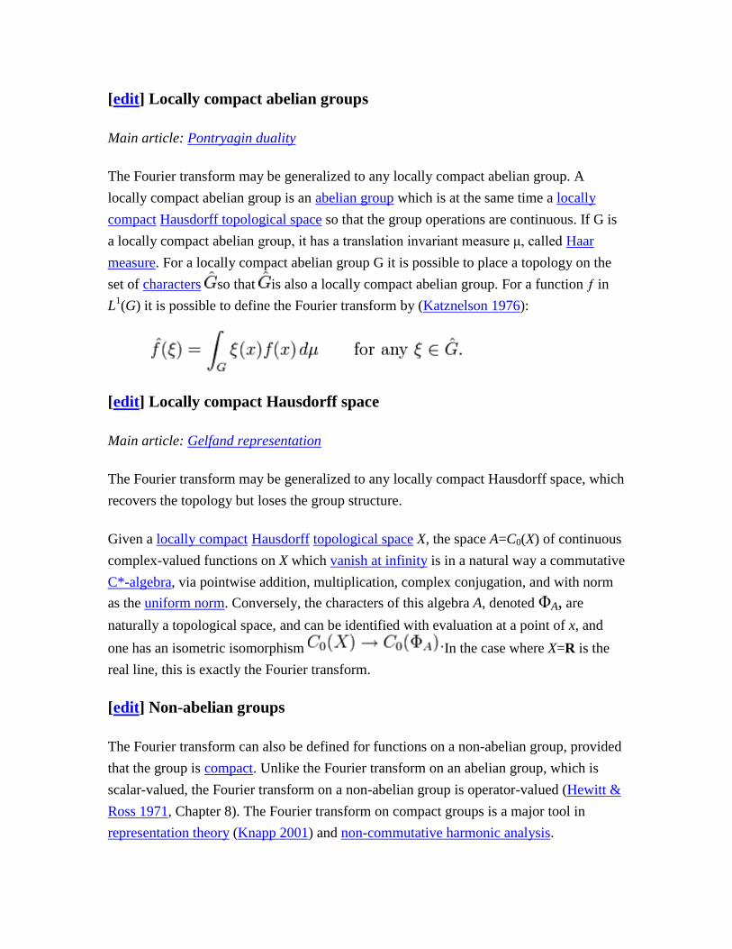
[edit] Locally compact abelian groups

Main article: Pontryagin duality

The Fourier transform may be generalized to any locally compact abelian group. A

locally compact abelian group is an abelian group which is at the same time a locally

compact Hausdorff topological space so that the group operations are continuous. If G is

a locally compact abelian group, it has a translation invariant measure μ, called Haar

measure. For a locally compact abelian group G it is possible to place a topology on the

set of characters so that is also a locally compact abelian group. For a function ƒ in

L1(G) it is possible to define the Fourier transform by (Katznelson 1976):

[edit] Locally compact Hausdorff space

Main article: Gelfand representation

The Fourier transform may be generalized to any locally compact Hausdorff space, which

recovers the topology but loses the group structure.

Given a locally compact Hausdorff topological space X, the space A=C0(X) of continuous

complex-valued functions on X which vanish at infinity is in a natural way a commutative

C*-algebra, via pointwise addition, multiplication, complex conjugation, and with norm

as the uniform norm. Conversely, the characters of this algebra A, denoted ΦA, are

naturally a topological space, and can be identified with evaluation at a point of x, and

one has an isometric isomorphism In the case where X=R is the

real line, this is exactly the Fourier transform.

[edit] Non-abelian groups

The Fourier transform can also be defined for functions on a non-abelian group, provided

that the group is compact. Unlike the Fourier transform on an abelian group, which is

scalar-valued, the Fourier transform on a non-abelian group is operator-valued (Hewitt &

Ross 1971, Chapter 8). The Fourier transform on compact groups is a major tool in

representation theory (Knapp 2001) and non-commutative harmonic analysis.

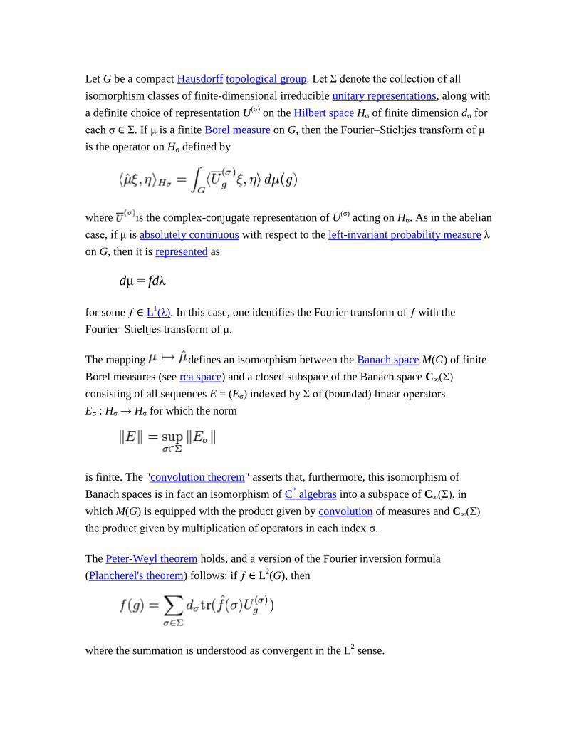
Let G be a compact Hausdorff topological group. Let Σ denote the collection of all

isomorphism classes of finite-dimensional irreducible unitary representations, along with

a definite choice of representation U(σ)

on the Hilbert space Hσ of finite dimension dσ for

each σ ∈ Σ. If μ is a finite Borel measure on G, then the Fourier–Stieltjes transform of μ

is the operator on Hσ defined by

where is the complex-conjugate representation of U(σ)

acting on Hσ. As in the abelian

case, if μ is absolutely continuous with respect to the left-invariant probability measure λ

on G, then it is represented as

dμ = fdλ

for some ƒ ∈ L1(λ). In this case, one identifies the Fourier transform of ƒ with the

Fourier–Stieltjes transform of μ.

The mapping defines an isomorphism between the Banach space M(G) of finite

Borel measures (see rca space) and a closed subspace of the Banach space C∞(Σ)

consisting of all sequences E = (Eσ) indexed by Σ of (bounded) linear operators

Eσ : Hσ → Hσ for which the norm

is finite. The "convolution theorem" asserts that, furthermore, this isomorphism of

Banach spaces is in fact an isomorphism of C* algebras into a subspace of C∞(Σ), in

which M(G) is equipped with the product given by convolution of measures and C∞(Σ)

the product given by multiplication of operators in each index σ.

The Peter-Weyl theorem holds, and a version of the Fourier inversion formula

(Plancherel's theorem) follows: if ƒ ∈ L2(G), then

where the summation is understood as convergent in the L2 sense.

The generalization of the Fourier transform to the noncommutative situation has also in

part contributed to the development of noncommutative geometry.[citation needed]

In this

context, a categorical generalization of the Fourier transform to noncommutative groups

is Tannaka-Krein duality, which replaces the group of characters with the category of

representations. However, this loses the connection with harmonic functions.

[edit] Alternatives

In signal processing terms, a function (of time) is a representation of a signal with perfect

time resolution, but no frequency information, while the Fourier transform has perfect

frequency resolution, but no time information: the magnitude of the Fourier transform at

a point is how much frequency content there is, but location is only given by phase

(argument of the Fourier transform at a point), and standing waves are not localized in

time – a sine wave continues out to infinity, without decaying. This limits the usefulness

of the Fourier transform for analyzing signals that are localized in time, notably

transients, or any signal of finite extent.

As alternatives to the Fourier transform, in time-frequency analysis, one uses time-

frequency transforms or time-frequency distributions to represent signals in a form that

has some time information and some frequency information – by the uncertainty

principle, there is a trade-off between these. These can be generalizations of the Fourier

transform, such as the short-time Fourier transform or fractional Fourier transform, or can

use different functions to represent signals, as in wavelet transforms and chirplet

transforms, with the wavelet analog of the (continuous) Fourier transform being the

continuous wavelet transform. (Boashash 2003). For a variable time and frequency

resolution, the De Groot Fourier Transform can be considered.

[edit] Applications

[edit] Analysis of differential equations

Fourier transforms and the closely related Laplace transforms are widely used in solving

differential equations. The Fourier transform is compatible with differentiation in the

following sense: if f(x) is a differentiable function with Fourier transform , then the

Fourier transform of its derivative is given by . This can be used to transform

differential equations into algebraic equations. Note that this technique only applies to

problems whose domain is the whole set of real numbers. By extending the Fourier

transform to functions of several variables partial differential equations with domain Rn

can also be translated into algebraic equations.

[edit] Fourier transform spectroscopy

Main article: Fourier transform spectroscopy

The Fourier transform is also used in nuclear magnetic resonance (NMR) and in other

kinds of spectroscopy, e.g. infrared (FTIR). In NMR an exponentially-shaped free

induction decay (FID) signal is acquired in the time domain and Fourier-transformed to a

Lorentzian line-shape in the frequency domain. The Fourier transform is also used in

magnetic resonance imaging (MRI) and mass spectrometry.

[edit] Domain and range of the Fourier transform

It is often desirable to have the most general domain for the Fourier transform as

possible. The definition of Fourier transform as an integral naturally restricts the domain

to the space of integrable functions. Unfortunately, there is no simple characterizations of

which functions are Fourier transforms of integrable functions (Stein & Weiss 1971). It is

possible to extend the domain of the Fourier transform in various ways, as discussed in

generalizations above. The following list details some of the more common domains and

ranges on which the Fourier transform is defined.

The space of Schwartz functions is closed under the Fourier transform. Schwartz

functions are rapidly decaying functions and do not include all functions which

are relevant for the Fourier transform. More details may be found in (Stein &

Weiss 1971).

The space Lp maps into the space L

q, where 1/p + 1/q = 1 and 1 ≤ p ≤ 2

(Hausdorff–Young inequality).

In particular, the space L2 is closed under the Fourier transform, but here the

Fourier transform is no longer defined by integration.

The space L1 of Lebesgue integrable functions maps into C0, the space of

continuous functions that tend to zero at infinity – not just into the space of

bounded functions (the Riemann–Lebesgue lemma).

The set of tempered distributions is closed under the Fourier transform. Tempered

distributions are also a form of generalization of functions. It is in this generality

that one can define the Fourier transform of objects like the Dirac comb.

[edit] Other notations

Other common notations for are these:

Though less commonly other notations are used. Denoting the Fourier transform by a

capital letter corresponding to the letter of function being transformed (such as f(x) and

F(ξ)) is especially common in the sciences and engineering. In electronics, the omega (ω)

is often used instead of ξ due to its interpretation as angular frequency, sometimes it is

written as F(jω), where j is the imaginary unit, to indicate its relationship with the

Laplace transform, and sometimes it is written informally as F(2πf) in order to use

ordinary frequency.

The interpretation of the complex function may be aided by expressing it in polar

coordinate form: in terms of the two real functions A(ξ) and φ(ξ)

where:

is the amplitude and

is the phase (see arg function).

Then the inverse transform can be written:

which is a recombination of all the frequency components of ƒ(x). Each component is a

complex sinusoid of the form e2πixξ

whose amplitude is A(ξ) and whose initial phase

angle (at x = 0) is φ(ξ).

The Fourier transform may be thought of as a mapping on function spaces. This mapping

is here denoted and is used to denote the Fourier transform of the function f.

This mapping is linear, which means that can also be seen as a linear transformation

on the function space and implies that the standard notation in linear algebra of applying

a linear transformation to a vector (here the function f) can be used to write instead of

. Since the result of applying the Fourier transform is again a function, we can be

interested in the value of this function evaluated at the value ξ for its variable, and this is

denoted either as or as . Notice that in the former case, it is implicitly

understood that is applied first to f and then the resulting function is evaluated at ξ, not

the other way around.

In mathematics and various applied sciences it is often necessary to distinguish between a

function f and the value of f when its variable equals x, denoted f(x). This means that a

notation like formally can be interpreted as the Fourier transform of the values

of f at x. Despite this flaw, the previous notation appears frequently, often when a

particular function or a function of a particular variable is to be transformed. For

example, is sometimes used to express that the Fourier

transform of a rectangular function is a sinc function, or

is used to express the shift property of the

Fourier transform. Notice, that the last example is only correct under the assumption that

the transformed function is a function of x, not of x0.

[edit] Other conventions

The Fourier transform can also be written in terms of angular frequency: ω = 2πξ whose

units are radians per second.

The substitution ξ = ω/(2π) into the formulas above produces this convention:

Under this convention, the inverse transform becomes:

Unlike the convention followed in this article, when the Fourier transform is defined this

way, it is no longer a unitary transformation on L2(R

n). There is also less symmetry

between the formulas for the Fourier transform and its inverse.

Another convention is to split the factor of (2π)n evenly between the Fourier transform

and its inverse, which leads to definitions:

Under this convention, the Fourier transform is again a unitary transformation on L2(R

n).

It also restores the symmetry between the Fourier transform and its inverse.

Variations of all three conventions can be created by conjugating the complex-

exponential kernel of both the forward and the reverse transform. The signs must be

opposites. Other than that, the choice is (again) a matter of convention.

Summary of popular forms of the Fourier transform

ordinary

frequency

ξ (hertz)

unitary

angular

frequency

ω (rad/s)

non-

unitary

unitary

The ordinary-frequency convention (which is used in this article) is the one most often

found in the mathematics literature.[citation needed]

In the physics literature, the two angular-

frequency conventions are more commonly used.[citation needed]

As discussed above, the characteristic function of a random variable is the same as the

Fourier–Stieltjes transform of its distribution measure, but in this context it is typical to

take a different convention for the constants. Typically characteristic function is defined

. As in the case of the "non-unitary angular frequency"

convention above, there is no factor of 2π appearing in either of the integral, or in the

exponential. Unlike any of the conventions appearing above, this convention takes the

opposite sign in the exponential.

[edit] Tables of important Fourier transforms

The following tables record some closed form Fourier transforms. For functions ƒ(x) ,

g(x) and h(x) denote their Fourier transforms by , , and respectively. Only the three

most common conventions are included. It may be useful to notice that entry 105 gives a

relationship between the Fourier transform of a function and the original function, which

can be seen as relating the Fourier transform and its inverse.

[edit] Functional relationships

The Fourier transforms in this table may be found in (Erdélyi 1954) or the appendix of

(Kammler 2000).

Function

Fourier transform

unitary, ordinary

frequency

Fourier transform

unitary, angular frequency

Fourier transform

non-unitary, angular

frequency

Remarks

Definition

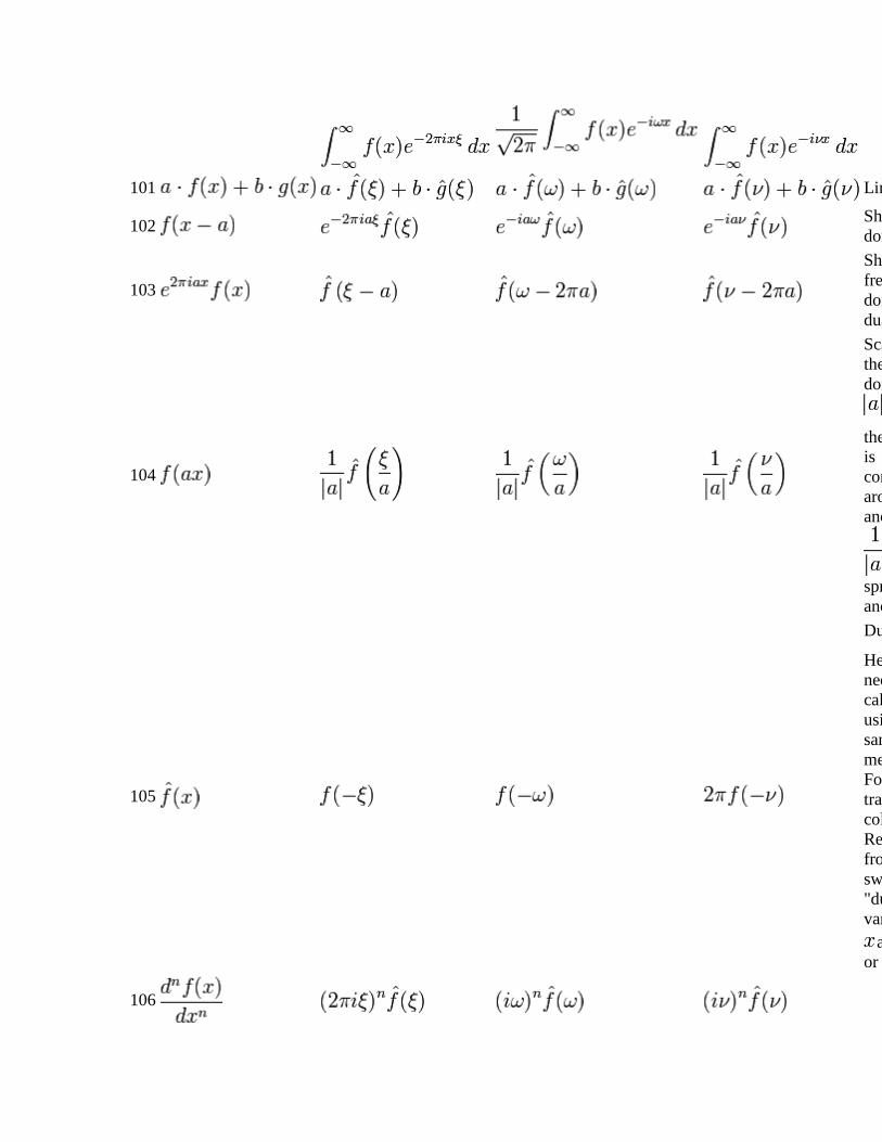
101

Linearity

102

Shift in time

domain

103

Shift in

frequency

domain,

dual of 102

104

Scaling in

the time

domain. If

is large,

then

is

concentrated

around 0

and

spreads out

and flattens.

105

Duality.

Here

needs to be

calculated

using the

same

method as

Fourier

transform

column.

Results

from

swapping

"dummy"

variables of

and or

or .

106

107

This is the

dual of 106

108

The notation

denotes the

convolution

of and —

this rule is

the

convolution

theorem

109

This is the

dual of 108

110 For a purely real

Hermitian

symmetry.

indicates

the complex

conjugate.

111 For a purely real

even function , and are purely real even functions.

112 For a purely real

odd function , and are purely imaginary odd functions.

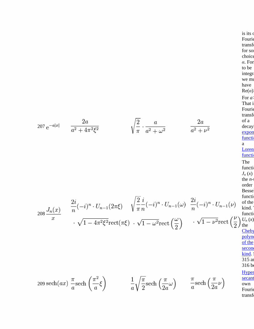
[edit] Square-integrable functions

The Fourier transforms in this table may be found in (Campbell & Foster 1948), (Erdélyi

1954), or the appendix of (Kammler 2000).

Function

Fourier transform

unitary, ordinary

frequency

Fourier transform

unitary, angular frequency

Fourier transform

non-unitary, angular

frequency

Remarks

201

The

rectangular

pulse and

the

normalized

sinc

function,

here

defined as

sinc(x) =

sin(πx)/(πx)

202

Dual of

rule 201.

The

rectangular

function is

an ideal

low-pass

filter, and

the sinc

function is

the non-

causal

impulse

response of

such a

filter.

203

The

function

tri(x) is the

triangular

function

204

Dual of

rule 203.

205

The

function

u(x) is the

Heaviside

unit step

function

and a>0.

206

This shows

that, for the

unitary

Fourier

transforms,

the

Gaussian

function

exp(−αx2)

is its own

Fourier

transform

for some

choice of

α. For this

to be

integrable

we must

have

Re(α)>0.

207

For a>0.

That is, the

Fourier

transform

of a

decaying

exponential

function is

a

Lorentzian

function.

208

The

functions

Jn (x) are

the n-th

order

Bessel

functions

of the first

kind. The

functions

Un (x) are

the

Chebyshev

polynomial

of the

second

kind. See

315 and

316 below.

209

Hyperbolic

secant is its

own

Fourier

transform

[edit] Distributions

The Fourier transforms in this table may be found in (Erdélyi 1954) or the appendix of

(Kammler 2000).

Function

Fourier transform

unitary, ordinary frequency

Fourier transform

unitary, angular frequency

Fourier transform

non-unitary, angular

frequency

Remarks

301

The distribution δ(ξ) denotes the Dirac

delta function.

302

Dual of rule 301.

303

This follows from 103 and 301.

304

This follows from rules 101 and 303

using Euler's formula:

305

This follows from 101 and 303 using

306

307

308

Here, n is a natural number and

is the n-th distribution derivative of the

Dirac delta function. This rule follows

from rules 107 and 301. Combining this

rule with 101, we can transform all

polynomials.

309

Here sgn(ξ) is the sign function. Note

that 1/x is not a distribution. It is

necessary to use the Cauchy principal

value when testing against Schwartz

functions. This rule is useful in studying

the Hilbert transform.

310

1/xn is the homogeneous distribution

defined by the distributional derivative

311

If Re α > −1, then | x | α is a locally

integrable function, and so a tempered

distribution. The function is a

holomorphic function from the right half-

plane to the space of tempered

distributions. It admits a unique

meromorphic extension to a tempered

distribution, also denoted | x | α for α ≠

−2, −4, ... (See homogeneous

distribution.)

312

The dual of rule 309. This time the

Fourier transforms need to be considered

as Cauchy principal value.

313

The function u(x) is the Heaviside unit

step function; this follows from rules

101, 301, and 312.

314

This function is known as the Dirac comb

function. This result can be derived from

302 and 102, together with the fact that

as distributions.

315

The function J0(x) is the zeroth order

Bessel function of first kind.

316

This is a generalization of 315. The

function Jn(x) is the n-th order Bessel

function of first kind. The function Tn(x)

is the Chebyshev polynomial of the first

kind.

[edit] Two-dimensional functions

Functions (400 to

402)

Fourier transform

unitary, ordinary frequency

Fourier transform

unitary, angular frequency

Fourier transform

non-unitary, angular frequency

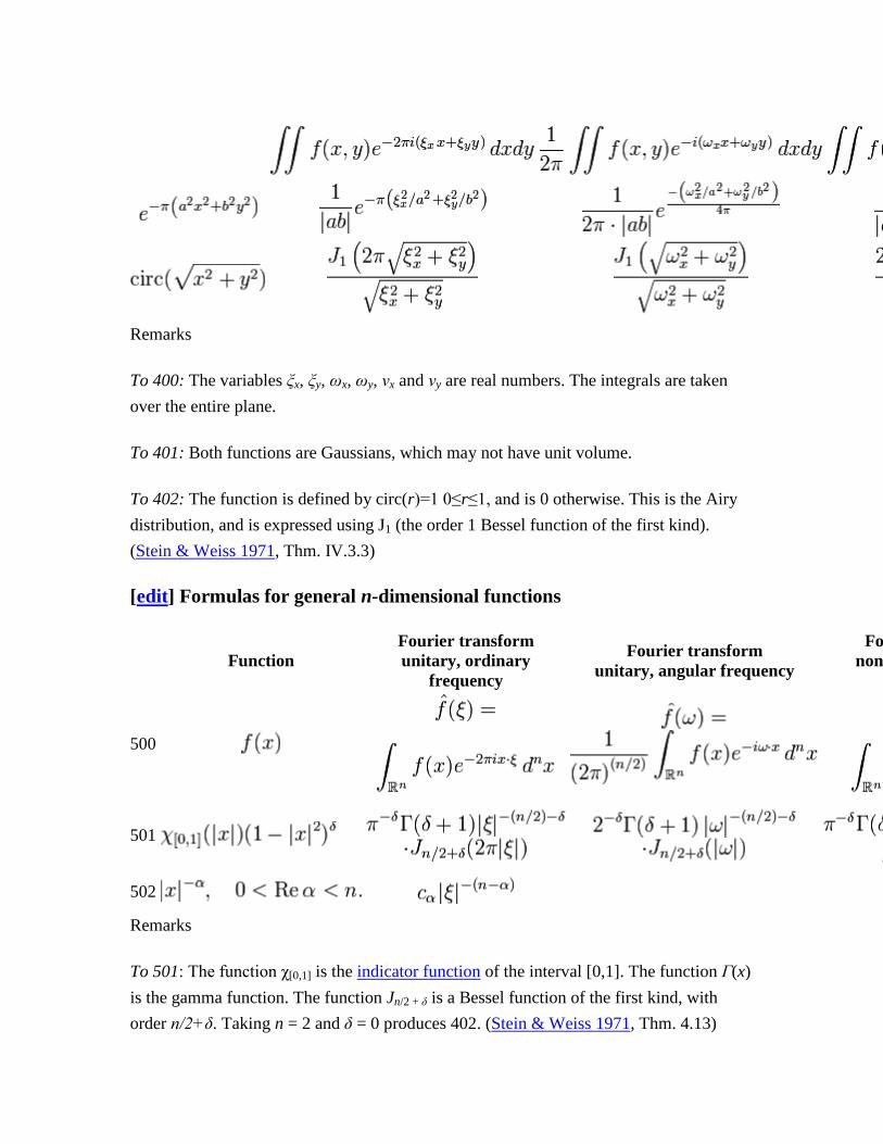
Remarks

To 400: The variables ξx, ξy, ωx, ωy, νx and νy are real numbers. The integrals are taken

over the entire plane.

To 401: Both functions are Gaussians, which may not have unit volume.

To 402: The function is defined by circ(r)=1 0≤r≤1, and is 0 otherwise. This is the Airy

distribution, and is expressed using J1 (the order 1 Bessel function of the first kind).

(Stein & Weiss 1971, Thm. IV.3.3)

[edit] Formulas for general n-dimensional functions

Function

Fourier transform

unitary, ordinary

frequency

Fourier transform

unitary, angular frequency

Fourier transform

non-unitary, angular

frequency

500

501

502

Remarks

To 501: The function χ[0,1] is the indicator function of the interval [0,1]. The function Γ(x)

is the gamma function. The function Jn/2 + δ is a Bessel function of the first kind, with

order n/2+δ. Taking n = 2 and δ = 0 produces 402. (Stein & Weiss 1971, Thm. 4.13)

To 502: See Riesz potential. The formula also holds for all α ≠ −n, −n−1, ... by analytic

continuation, but then the function and its Fourier transforms need to be understood as

suitably regularized tempered distributions. See homogeneous distribution.

[edit] See also

Fourier series

Fast Fourier transform

Laplace transform

Discrete Fourier transform

o DFT matrix

Discrete-time Fourier transform

Fourier–Deligne transform

Fractional Fourier transform

Linear canonical transform

Fourier sine transform

Space-time Fourier transform

Short-time Fourier transform

Fourier inversion theorem

Analog signal processing

Transform (mathematics)

Integral transform

o Hartley transform

o Hankel transform

Symbolic integration

[edit] References

Boashash, B., ed. (2003), Time-Frequency Signal Analysis and Processing: A

Comprehensive Reference, Oxford: Elsevier Science, ISBN 0080443354

Bochner S., Chandrasekharan K. (1949), Fourier Transforms, Princeton

University Press

Bracewell, R. N. (2000), The Fourier Transform and Its Applications (3rd ed.),

Boston: McGraw-Hill, ISBN 0071160434.

Campbell, George; Foster, Ronald (1948), Fourier Integrals for Practical

Applications, New York: D. Van Nostrand Company, Inc..

Duoandikoetxea, Javier (2001), Fourier Analysis, American Mathematical

Society, ISBN 0-8218-2172-5.

Dym, H; McKean, H (1985), Fourier Series and Integrals, Academic Press,

ISBN 978-0122264511.

Erdélyi, Arthur, ed. (1954), Tables of Integral Transforms, 1, New Your:

McGraw-Hill

Fourier, J. B. Joseph (1822), Théorie Analytique de la Chaleur, Paris,

http://books.google.com/?id=TDQJAAAAIAAJ&printsec=frontcover&dq=Th%C

3%A9orie+analytique+de+la+chaleur&q

Grafakos, Loukas (2004), Classical and Modern Fourier Analysis, Prentice-Hall,

ISBN 0-13-035399-X.

Hewitt, Edwin; Ross, Kenneth A. (1970), Abstract harmonic analysis. Vol. II:

Structure and analysis for compact groups. Analysis on locally compact Abelian

groups, Die Grundlehren der mathematischen Wissenschaften, Band 152, Berlin,

New York: Springer-Verlag, MR0262773.

Hörmander, L. (1976), Linear Partial Differential Operators, Volume 1, Springer-

Verlag, ISBN 978-3540006626.

James, J.F. (2002), A Student's Guide to Fourier Transforms (2nd ed.), New

York: Cambridge University Press, ISBN 0-521-00428-4.

Kaiser, Gerald (1994), A Friendly Guide to Wavelets, Birkhäuser, ISBN 0-8176-

3711-7

Kammler, David (2000), A First Course in Fourier Analysis, Prentice Hall,

ISBN 0-13-578782-3

Katznelson, Yitzhak (1976), An introduction to Harmonic Analysis, Dover,

ISBN 0-486-63331-4

Knapp, Anthony W. (2001), Representation Theory of Semisimple Groups: An

Overview Based on Examples, Princeton University Press, ISBN 978-0-691-

09089-4, http://books.google.com/?id=QCcW1h835pwC

Pinsky, Mark (2002), Introduction to Fourier Analysis and Wavelets,

Brooks/Cole, ISBN 0-534-37660-6

Polyanin, A. D.; Manzhirov, A. V. (1998), Handbook of Integral Equations, Boca

Raton: CRC Press, ISBN 0-8493-2876-4.

Rudin, Walter (1987), Real and Complex Analysis (Third ed.), Singapore:

McGraw Hill, ISBN 0-07-100276-6.

Stein, Elias; Shakarchi, Rami (2003), Fourier Analysis: An introduction,

Princeton University Press, ISBN 0-691-11384-X.

Stein, Elias; Weiss, Guido (1971), Introduction to Fourier Analysis on Euclidean

Spaces, Princeton, N.J.: Princeton University Press, ISBN 978-0-691-08078-9.

Wilson, R. G. (1995), Fourier Series and Optical Transform Techniques in

Contemporary Optics, New York: Wiley, ISBN 0471303577.

Yosida, K. (1968), Functional Analysis, Springer-Verlag, ISBN 3-540-58654-7.

[edit] External links

Fourier Transform Tutorial

Fourier Series Applet (Tip: drag magnitude or phase dots up or down to change

the wave form).

Stephan Bernsee's FFTlab (Java Applet)

Stanford Video Course on the Fourier Transform

Tables of Integral Transforms at EqWorld: The World of Mathematical

Equations.

Weisstein, Eric W., "Fourier Transform" from MathWorld.

Fourier Transform Module by John H. Mathews

The DFT ―à Pied‖: Mastering The Fourier Transform in One Day at The DSP

Dimension

An Interactive Flash Tutorial for the Fourier Transform

Categories: Fundamental physics concepts | Fourier analysis | Integral transforms |

Unitary operators | Joseph Fourier

Hidden categories: All articles with unsourced statements | Articles with unsourced

statements from May 2009 | Articles with unsourced statements from July 2009

Personal tools

Log in / create account

Namespaces

Article

Discussion

Variants

Views

Read

Edit

View history

Actions

Search

Navigation

Main page

Contents

Featured content

Current events

Random article

Donate to Wikipedia

Interaction

Help

About Wikipedia

Community portal

Recent changes

Contact Wikipedia

Toolbox

What links here

Related changes

Upload file

Special pages

Permanent link

Cite this page

Print/export

Create a book

Download as PDF

Printable version

Languages

አማርኛ

العربية

Беларуска (тара ке а)

Català

Česky

Dansk

Deutsch

Eesti

Español

Esperanto

Euskara

فارسی

Français

Galego

한국어

Bahasa Indonesia

Íslenska

Italiano

עברית

Lietuvių

Magyar

Malti

Nederlands

日本語

Norsk (bokm l)

Norsk (nynorsk)

Polski

Português

Română

Русский

Shqip

Simple English

Slovenčina

Српски / Srpski

Basa Sunda

Suomi

Svenska

தமிழ்

ไทย Türkçe

Українська

Tiếng Việt

中文

This page was last modified on 11 April 2011 at 19:29.

Text is available under the Creative Commons Attribution-ShareAlike License;

additional terms may apply. See Terms of Use for details.

Wikipedia® is a registered trademark of the Wikimedia Foundation, Inc., a non-

profit organization.

Contact us

Privacy policy

About Wikipedia

Disclaimers