1

FOURIER TRANSFORM METHODS David Sandwell, January, 2013

1. Fourier Transforms Fourier analysis is a fundamental tool used in all areas of science and engineering. The fast

fourier transform (FFT) algorithm is remarkably efficient for solving large problems. Nearly

every computing platform has a library of highly-optimized FFT routines. In the field of Earth

science, fourier analysis is used in the following areas:

Solving linear partial differential equations (PDE’s):

Gravity/magnetics Laplace ∇2Φ = 0

Elasticity (flexure) Biharmonic ∇4Φ = 0

Heat Conduction Diffusion ∇2Φ - δ Φ/ δt = 0

Wave Propagation Wave ∇2Φ - δ2Φ/ δt2 = 0

Designing and using antennas:

Seismic arrays and streamers

Multibeam echo sounder and side scan sonar

Interferometers – VLBI – GPS

Synthetic Aperture Radar (SAR) and Interferometric SAR (InSAR)

Image Processing and filters:

Transformation, representation, and encoding

Smoothing and sharpening

Restoration, blur removal, and Wiener filter

Data Processing and Analysis:

High-pass, low-pass, and band-pass filters

Cross correlation – transfer functions – coherence

Signal and noise estimation – encoding time series

2

Figure 1.1 Cartesian coordinate system used throughout the book with z positive up. The z = 0 plane is the surface of the earth. Fourier transforms deal with infinite domains while the fourier series (section 1.6) has finite domains. For our numerical examples we will select an area of length L and with W consisting of uniform cells of size Δx and Δy . This can be represented as a 2-D array of numbers with J = L /Δx columns and I =W /Δy rows.

1.1 Definitions of fourier transforms

The 1-dimensional forward and inverse fourier transforms are defined as:

F k( ) = f x( )−∞

∞

∫ e−i2πkxdx or F k( ) =ℑ f x( )%& '( (1.1)

f x( ) = F k( )−∞

∞

∫ ei2πkxdk or f x( ) =ℑ−1 F k( )%& '( (1.2)

where x is distance and k is wavenumber where k =1/ λ and λ is wavelength. We also use the

shorthand notation introduced by Bracewell [1978]. These equations are more commonly

written in terms of time t and frequency ν where ν =1/T and T is the period. The 2-

dimensional forward and inverse fourier transforms are defined as:

F k( ) = f x( )−∞

∞

∫−∞

∞

∫ e−i2πk•xd 2x or F k( ) =ℑ2 f x( )%& '( (1.3)

3

f x( ) = F k( )−∞

∞

∫−∞

∞

∫ ei2πk•xd 2k or f x( ) =ℑ2−1 F k( )%& '( (1.4)

where x = x, y( ) is the position vector, k = kx,ky( ) is the wavenumber vector, and

k • x = kxx + kyy . The magnitude of the spatial wavenumber β = kx2 + ky

2( )1/2

is used often in later

chapters. For several of the derivations, we’ll also take the fourier transform in the z-direction

(i.e. 3-D transform) using the following notation.

F kz( ) = f z( )−∞

∞

∫ e−i2πkzzdz (1.5)

f z( ) = F kz( )−∞

∞

∫ ei2πkzzdkz (1.6)

Fourier transformation with respect to time is also sometimes used to form a 4-D transform.

F ν( ) = f t( )−∞

∞

∫ e−i2πνtdt (1.7)

f t( ) = F ν( )−∞

∞

∫ ei2πνtdν (1.8)

While algebraic manipulation of equations in 4-D is sometimes challenging and error prone,

we’ll use computers to help us in two ways. We’ll use the tools of computer algebra to solve the

most challenging algebraic manipulations associated with the 3-D and 4-D problems in chapter

4. In addition we’ll provide a FORTRAN subroutine called fourt() which can perform numerical

fourier transforms in N-dimensions although we’ll use only 1-, 2-, and 3-D numerical transforms

in this book.

1.2 Fourier sine and cosine transforms

Here we introduce the sine and cosine transforms to illustrate the transforms of odd and even

functions. Also in later chapters we’ll use sine and cosine transforms to match asymmetric and

symmetric boundary conditions for particular models.

4

Any function f x( ) can be decomposed into odd O x( ) and even E x( ) functions such that

f x( ) = E x( )+O x( ) (1.9)

where E x( ) = 12f x( )+ f −x( )"# $% and O x( ) = 1

2f x( )− f −x( )"# $% . Note the complex exponential

function can be written as

eiθ = cos θ( )+ isin θ( ) (1.10)

Exercise 1.1 Use equation (1.10) to show that cos θ( ) = 12eiθ + e−iθ( ) and sin θ( ) = 1

2ieiθ − e−iθ( ) .

Using this expression (1.10) we can write the forward 1-D transform as the sum of two parts

F k( ) = f x( )−∞

∞

∫ cos 2πkx( )dx − i f x( )−∞

∞

∫ sin 2πkx( )dx (1.11)

After inserting equation (1.9) into this expression and noting that the integral of an odd function

times an even function is zero, we arrive at the expressions for the cosine and sine transforms.

F k( ) = 2 E x( )0

∞

∫ cos 2πkx( )dx − 2i O x( )0

∞

∫ sin 2πkx( )dx (1.12)

Throughout this book we’ll be dealing with real-valued functions. From equation (1.12) it is

evident that the cosine transform of a real, even function is also real and even. Also the sine

transform of a real odd function is imaginary and odd. In other words when a function in the

space domain is real valued, its fourier transform F k( ) has a special Hermitian property

F k( ) = F −k( )* so one can reconstruct the transform of the function with negative wavenumbers

from the transform with positive wavenumbers. Later when we perform numerical examples

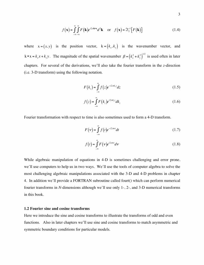
5

using real valued functions such as topography, we can use this Hermitian property to reduce the

memory allocation for the fourier transformed array by a factor of 2. This is important for large

2-D and 3-D transforms.

1.3 Examples of Fourier Transforms

Throughout the book we will work with only linear partial differential equations so all the

problems are separable and the order of differentiation and integration is irrelevant. For example

the 2-D fourier transform of is given by

F kx,ky( ) = f x, y( )e−i2πkxx dx−∞

∞

∫$

%&

'

()

−∞

∞

∫ e−i2πkyydy = f x, y( )e−i2πkyy dy−∞

∞

∫$

%&

'

()

−∞

∞

∫ e−i2πkxxdx (1.13)

Note that this 2-D transform consists of a sequence of 1-D transforms. This property can be

extended to 3-D, 4-D and even N-D; each transform can be performed separately and

independently of the transforms in the other dimensions. In the following analysis we’ll only

show examples of 1-D transforms but the extension to higher dimensions is trivial.

Delta function – By definition the delta function has the following property;

f x( )−∞

∞

∫ δ x − a( )dx ≡ f a( ) (1.14)

under integration it extracts the value of f x( ) at the position x = a . One can describe the delta

function as having infinite height at zero argument and zero height elsewhere. The area under

the delta function is 1. In terms of pure mathematics the delta function is not a function and only

has meaning when integrated against another function. In this book we use the delta function as

a powerful tool, provided to us by the mathematicians, so we trust all the mathematical theory

behind it. What is the fourier transform of a delta function? By definition if one performs a

forward transform of a function followed by an inverse transform, or vice versa, one will arrive

back with the original function. Lets try this using the delta function. By definition, the inverse

transform of a delta function is

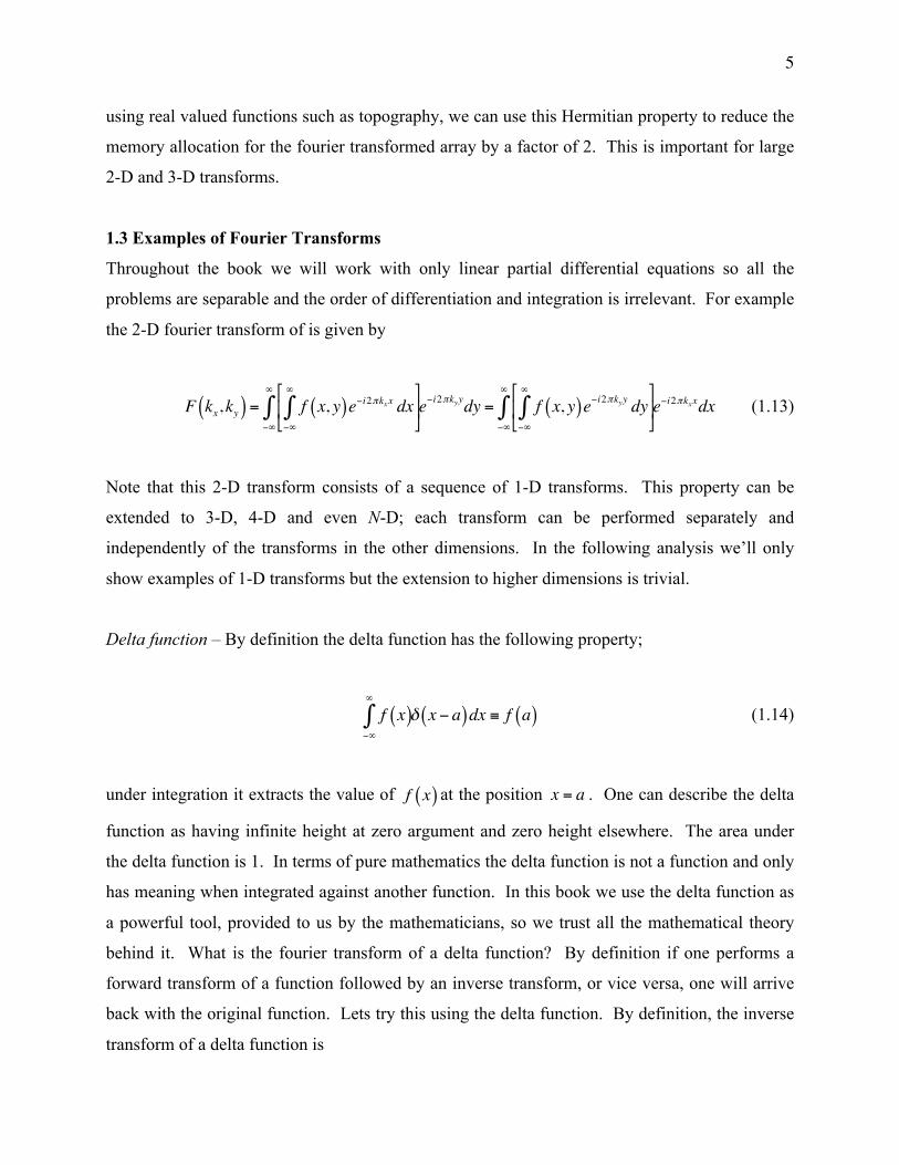
6

δ k − ko( )−∞

∞

∫ ei2πkxdk = ei2πkox (1.15)

Next lets take the forward transform of equation (1.15). The left hand side will be the delta

function because we have performed an inverse and forward transform. The right hand side is

given by

δ k − ko( ) = ei2πkox−∞

∞

∫ e−i2πkxdx = e−i2π k−ko( )x dx−∞

∞

∫ (1.16)

This result shows that the fourier basis functions are orthonormal. If we consider the special

case of ko = 0we see that the fourier transform of a delta function is ℑ δ k( )"# $%=1 . Since fourier

transformation is reciprocal in distance x and wavenumber k, it is also true that ℑ δ x( )"# $%=1 . The

delta function and its fourier transform provide an amazingly powerful tool for solving linear

PDEs.

Cosine and sine functions – Lets use the delta function tool and the expressions from Exercise

1.1 to calculate the fourier transform of a cosine function having a single wavenumber

cos 2πk0x( ) .

cos 2πkox( )−∞

∞

∫ e−i2πkxdx = 12

ei2πkox + e−i2πkox +( )−∞

∞

∫ e−i2πkxdx = 12δ k − ko( )+δ k + ko( )$% &' (1.17)

So the fourier transform of a cosine function is simply two delta functions located at ±ko .

Exercise 1.2 Show that the Fourier transform of sin 2πk0x( ) is 12i

δ k − ko( )−δ k + ko( )"# $% .

7

Gaussian function – The Gaussian e−π x2

function also plays a fundamental role in solutions to

several types of PDEs. Its fourier transform is

F k( ) = e−π x2

e−i2πkx−∞

∞

∫ dx = e−π x2+i2kx( )

−∞

∞

∫ dx (1.18)

Note that x + ik( )2 = x2 + i2kx( )− k2 . Using this we can rewrite equation (1.18) as

F(k) = e−πk2

e−π x+ik( )2

−∞

∞

∫ dx = e−πk2

e−π x+ik( )2

−∞

∞

∫ d x + ik( ) = e−πk2 (1.19)

where we have used the result that the infinite integral of e−π x2

is 1. This is a remarkable and

powerful result that the fourier transform of a Gaussian is simply a Gaussian.

8

Figure 1.2 Schematic plots of 1-D fourier transform pairs. Solid line is real-valued function

while dashed line is imaginary valued function (figure from Bracewell [1978].

1.4 Properties of fourier transforms

There are several properties of fourier transforms that can be used as tools for solving PDEs.

The first property called the similarity property says that if you scale a function by a factor of a

along the x-axis, its fourier transform will scaled by a−1 along the k-axis and the amplitude will

be scaled by a −1 .

9

Exercise 1.3 Use the definition of the fourier transform equation (1.1) and a change of variable

to show the following. Try positive and negative values for a to understand why the absolute

value is needed in the amplitude scaling.

ℑ f ax( )"# $%=1aF k

a&

'()

*+ (1.20)

The shift property says that the fourier transform of a function that is shifted by a along the x-

axis equals the original fourier transform scaled by a phase factor. This property is especially

useful for numerically shifting a function a non-integer amount of the data spacing along the

axis.

Exercise 1.4 Use the definition of the fourier transform and a change of variable to show the

following

ℑ f x − a( )#$ %&= e−i2πkaF k( ) (1.21)

The derivative property of the fourier transform is the essential tool used in this book to

transform linear PDEs into algebraic equations that are easily solved. It states that the fourier

transform of the derivative of a function is the fourier transform of the original function scaled

by the imaginary wavenumber.

ℑ∂f∂x#

$%&

'(= i2πkF k( ) (1.22)

To show this is true we start with the inverse transform of equation (1.22)

∂f∂x

= i2πk−∞

∞

∫ F k( )ei2πkxdk (1.23)

Next take the forward transform of equation (1.23) and rearrange terms

10

ℑ∂f∂x#

$%&

'(= i2πko

−∞

∞

∫−∞

∞

∫ F ko( )ei2πkoxdkoe−i2πkxdx = i2πko−∞

∞

∫ F ko( ) e−i2π k−ko( )x

−∞

∞

∫ dx,-.

/01dko (1.24)

The term in the curly brackets is the delta function δ k − ko( )given in equation (1.16). The result

is

ℑ∂f∂x#

$%&

'(= i2πko

−∞

∞

∫ F ko( )δ k − ko( )dko = i2πkF k( ) (1.25)

The final property considered here is the convolution theorem which states that the fourier

transform of the convolution of two functions is equal to the product of the fourier transforms of

the original functions.

ℑ f u( )g x −u( )du−∞

∞

∫%

&'

(

)*= F k( )G k( ) (1.26)

To show this is true one can perform the fourier integration on the left side of equation (1.26)

and rearrange the order of the integrations

ℑ f u( )g x −u( )du−∞

∞

∫%

&'

(

)*= f u( )g x −u( )du

−∞

∞

∫%

&'

(

)*

−∞

∞

∫ e−i2πkxdx = f u( ) g x −u( )e−i2πkx dx−∞

∞

∫+,-

./0−∞

∞

∫ du (1.27)

Next use the shift property of the fourier transform to note that the function in the curly brackets

on the right side of equation (1.27) is e−i2πkuG k( ) . The result becomes

ℑ f u( )g x −u( )du−∞

∞

∫%

&'

(

)*=G k( ) f u( )

−∞

∞

∫ e−i2πkudu = F k( )G k( ) (1.28)

11

Note that these 4 properties are equally valid in 2-dimensions or even N-dimensions. The

properties also apply to discrete data. See Chapter 18 in Bracewell [1978].