Embed Size (px)
Citation preview

APPENDIXA
FOURIER TRANSFORM
In Chap. 2 we show that the Fourier transform plays an important role in analyzing LTI systems. Appendix A summarizes some of the important properties of Fourier transforms and their numerical calculation.
A.1. PROPERTIES OF THE FOURIER TRANSFORM
A functionftt) and its Fourier transform F(w) are related by the Fourier transform pair:
fco
F(w) = f f(t) exp(iwt)dt
fco
f(t) =_1 f F(w)exp(-iwt)dw 2n
We denote the relationship between these functions symbolically as:
f(t) B F(w)
(A.l)
(A.2)
(A.3)
Using the definition of the Fourier transform, we can show that the following relationships also exist
• Differentiation
provided
f(rn)(t) -7 0 as Itl-7 00 m =0, ... n-l 517
518
where
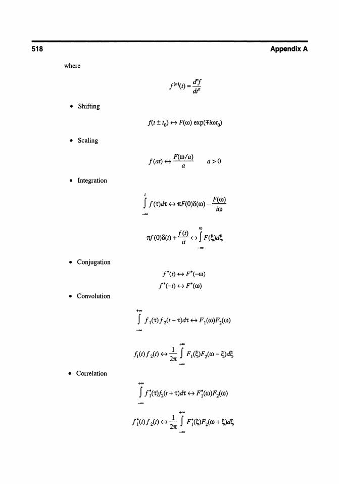
• Shifting
• Scaling
• Integration
• Conjugation
• Convolution
• Correlation
f(at) H F(oo/a) a > 0 a
t
f f(-c)d-c H nF(O)cS(oo) _ F~OO) zOO
+co
w
nf(O)cS(t) +~ H f F@d~ zt
I*(t) H F·(-(j)
!*(-t) H F*(w)
f f l(-c)f 2(t - -c)d-c H F1(oo)F2(oo)
+co
f1(t)f 2(t) H _1 f F1@F2(w - ~)d~ 2n
+co
f f~(-c)Ht + -c)d-c H F~(oo)F2(OO)
+co
f~(t)f 2(t) H _1 f F~(~)F2(OO + ~)d~ 2n
AppendixA

Fourier Transform
• Parsevals ' theorem
+00 +00
When
f f~('r)f 2('t)d't = _1 f F;(w)F2(W)dw 2n
+00 +00
f If(t)12dt = _I f IF(w)12dw 2n
A.2. SOME FOURIER TRANSFORM PAIRS
f(t)
1. Dirac delta function
5(t)
2. Heaviside step function
H(t) = {I t>O o t<O
3. Sign function
{I t> 0
sgn(t) = -1 t<O
4.ltl 1
5.(
6. exp( -at)H(t)
7. Laplace function
exp(-altl)
8. Gauss function
exp(-ar2)
9. Rectangular function
TI(t) = {~
sin(at) 10.--
nt
Itl< 1/2
ItI> 1/2
11. Triangular function
I\(t) = {b -Itl Itl:5 1
Itl> 1
F(oo)
i 1t5(00) +-
00
(2i/00)
(- 2/(02)
insgn(oo)
(a + ioo)/(a2 + (02)
sin(w/2) ---= sinqoo/21t) 00/2
TI(oo/2a)
519
520 AppendixA
A.3. DISCRETE FOURIER TRANSFORM
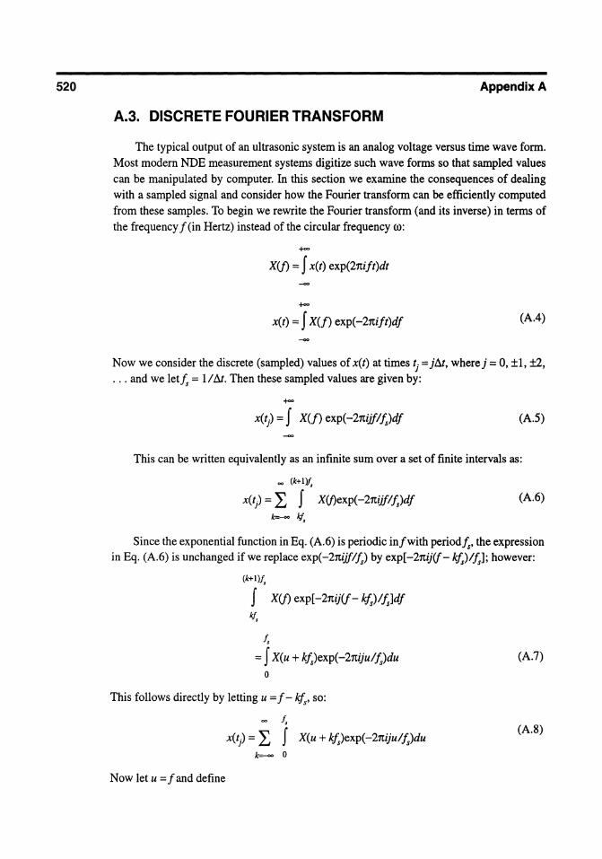
The typical output of an ultrasonic system is an analog voltage versus time wave form. Most modern NDE measurement systems digitize such wave forms so that sampled values can be manipulated by computer. In this section we ex amine the consequences of dealing with a sampled signal and consider how the Fourier transform can be efficiently computed from these sampIes. To begin we rewrite the Fourier transform (and its inverse) in terms of the frequency f(in Hertz) instead ofthe circular frequency (0:
+00
X(j) = f x(t) exp(21tift)dt
+00
x(t) = f X(f) exp(-21tift)df (A.4)
Now we consider the discrete (sampled) values of x(t) at times tj = jät, wherej = 0, ±1, ±2, ... and we letfs = 11M Then these sampled values are given by:
x(t) = f X(f) exp(-21tijf/fs)df (A.5)
This can be written equivalently as an infinite sum over a set of finite intervals as:
00 (k+ Ilf,
x(t) = L f X(f)exp(-21tijf/fs)df (A.6)
Since the exponential function in Eq. (A.6) is periodic infwith periodfs, the expression in Eq. (A.6) is unchanged if we replace exp(-21tijflfs) by exp[-21tij(f - kfs)lfs]; however:
(k+ 1 lf,
f X(j) exp[-21tij(f- kfs)lfs]df
kJ,
f,
= f X(u + kfs)exp(-21tijulfs)du o
This follows directly by letting u = f - kfs, so:
Now let u = fand define
00 J,
x(t) = L f X(u + kfs)exp(-21tijulfs)du Jc=.-co 0
(A.7)
(A.8)
Fourier Transform
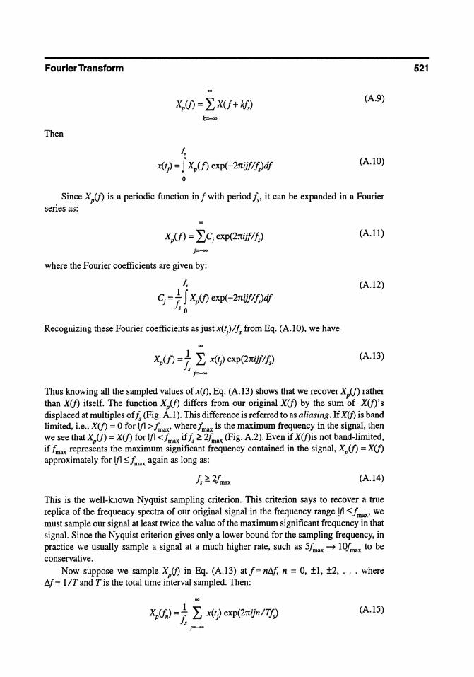
X/i) = L X(f + kf) (A.9)
Then
f,
x(t) = f Xi!) exp(-21tijflls)df (A.IO)
o
Since X/i) is a periodic function in f with period Is, it can be expanded in a Fourier series as:
(A.ll)
j=--
where the Fourier coefficients are given by:
f,
Cj = * f X/i) exp(-21tijfl ls)df s 0
(A.12)
Recognizing these Fourier coefficients as just x(911s from Eq. (A.IO), we have
Xi!) = 1. L x(9 exp(21tijf!ls) s .
(A.13)
J=--
Thus knowing all the sampled values of x(t) , Eq. (A.13) shows that we recover X/i) rather than X(j) itself. The function Xp(j) differs from our original X(j) by the sum of X(j)'s displaced at multiples ofls (Fig. A.l). This difference is referred to as aliasing. If X(j) is band limited, i.e., X(f) = 0 for Ijl > f max, wherefmax is the maximum frequency in the signal, then we see that Xp(j) = X(j) for Ifl <fmax ifls ~ 2fmax (Fig. A.2). Even if X(j)is not band-lirnited, if f max represents the maximum significant frequency contained in the signal, Xp(j) = X(f) approximately for Ifl ~fmax again as long as:
(A.14)
This is the well-known Nyquist sampling criterion. This criterion says to recover a true replica of the frequency spectra of our original signal in the frequency range !fl ~fmax' we must sampie our signal at least twice the value of the maximum significant frequency in that signal. Since the Nyquist criterion gives only a lower bound for the sampling frequency, in practice we usually sampie a signal at a much higher rate, such as 5fmax ~ lOfmax to be conservative.
Now suppose we sampie Xp(j) in Eq. (A.13) at f= n/:;,.f, n = 0, ±l, ±2, ... where /:;,.f = I IT and T is the total time interval sampled. Then:
X/fn) = 1. L x(9 exp(21tijnITIs) s .
j=--
(A.15)
521

522 AppendixA
X(j)
---=---L---.:::=------f
(b) fs f
Fig. A.1. (a) Fourier transform spectra X(f) and (b) its infinitely repeated periodic replica Xp(f).
However if we take Tfs = N, where N is an integer, and use the fact that exp(2nijn/N) is periodic inj with period N, we can rewrite Xifn) as:
where
N-l
X/In) = ~ L xp(9 exp(2nijn/N) j=O
(b)
(A.16)
Fig. A.2. (a) Fourier transform spectra X(f) of a band-limited function and (b) its infinitely repeated replica Xp(f) ifis> 2fmax.
Fourier Transform
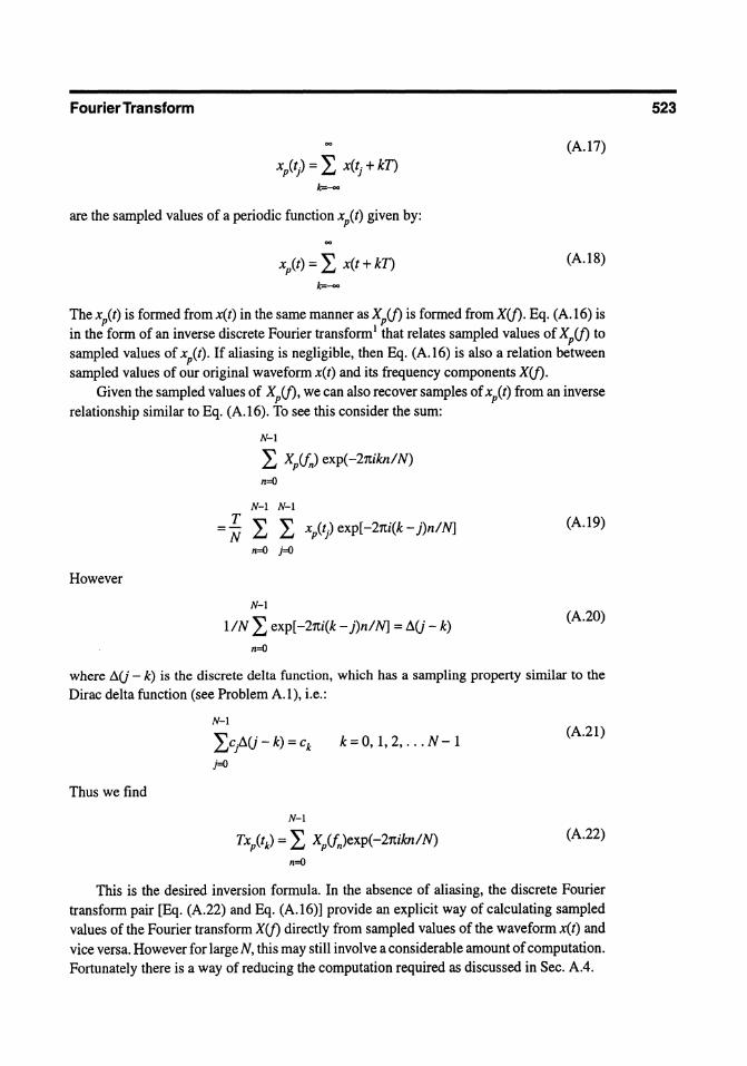
xp(9 = L x(tj + k1) k=-
are the sampled values of aperiodic function xit) given by:
(A.I7)
(A.IS)
Thexit) is formed fromx(t) in the same manner asX/i) is formed fromX(f). Eq. (A.I6) is in the form of an inverse discrete Fourier transformi that relates sampled values of Xp(f) to sampled values of xit). If aliasing is negligible, then Eq. (A.I6) is also a relation between sampled values of our original waveform x(t) and its frequency components X(f).
Given the sampled values of Xp(f), we can also recover sampIes of xp(t) from an inverse relationship sirnilar to Eq. (A.I6). To see this consider the sum:
However
N-l
LX/In) exp(-2TCiknIN) n=O
N-l N-l
- ~ L L xitj) exp[-2TCi(k - j)nlN] n=O j=O
N-l
l/N L exp[-2TCi(k - })nlN] = aU - k) n=O
(A.I9)
(A.20)
where AU - k) is the discrete delta funetion, which has a sampling property similar to the Dirae delta function (see Problem A.I), i.e.:
Thus we find
N-l
LcpU-k)=ck
j=O
N-l
k = 0, I, 2, ... N - I
Txitk) = L X/fn)exp(-2TCiknIN) n=O
(A.2I)
(A.22)
This is the desired inversion formula. In the absence of aliasing, the discrete Fourier transform pair [Eq. (A.22) and Eq. (A.I6)] provide an explicit way of calculating sampled values of the Fourier transform X(f) directly from sampled values of the waveform x(t) and vice versa. However for large N, this may still involve a considerable amount of computation. Fortunately there is a way of reducing the computation required as discussed in Sec. A.4.
523
524
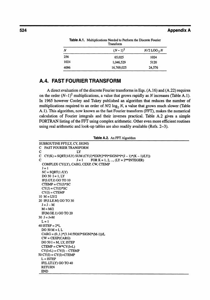
Table A.1. Multiplications Needed to Perform the Discrete Fourier Transform
N
256
1024
4096
65,025
1,046,529
16,769,025
A.4. FAST FOURIER TRANSFORM
1024
5120
24,576
AppendixA
A direct evaluation of the discrete Fourier transforrns in Eqs. (A.16) and (A.22) requires on the order (N-l f multiplications, a value that grows rapidly as N increases (Table A.l). In 1965 however Cooley and Tukey published an algorithm that reduces the number of multiplications required to an order of N/2 log2 N, a value that grows much slower (Table A.I). This algorithm, now known as the fast Fourier transforrn (FFT), makes the numerical calculation of Fourier integrals and their inverses practical. Table A.2 gives a simple FORTRAN listing of the FFT using complex arithmetic. Other even more efficient routines using real arithmetic and look-up tables are also readily available (Refs. 2-3).
SUBROUTINE FFT(LY, CY, SIGNI) C FAST FOURIER TRANSFORM C LY
Table A.2. An FFT Algorithrn
C CY(K) = SQRT(l/LY) SUM (CY(J)*EXP(2*PI*SIGNI*I*(J - I)*(K - I)/LY» C J = 1 FOR K = 1,2, ... , (LY = 2**INTEGER)
COMPLEX CY(LY), CARG, CEXP, CW, CTEMP J=I SC = SQRT(l./LY) D030 1= I,LY IF(I.GTJ) GO TO 10 CTEMP = CY(J)*SC CY(J) = CY(I)*SC CY(I) = CTEMP
10 M=LYI2 20 IF(J.LE.M) GO TO 30
J=J-M M=Ml2 IF(M.GE.l) GO TO 20
30 J=J+M L=I
40 ISTEP = 2*L DO 50M=I, L CARG = (0.,1.)*(3.14159265*SIGNI*(M-I»/L CW = CEXP(CARG) DO 50 I = M, LY, ISTEP CTEMP = CW*CY(I+L) CY(I+L) = CY(I) - CTEMP
50 CY (I) = CY (I)+CTEMP L=ISTEP IF(L.LT.LY) GO TO 40 RETURN END

FourierTransform
A.5. PROBLEMS
A.I. Define the discrete delta function 11 as:
l1(k- n) = {~ k=n k#:n
From this definition the sampling property ofthe discrete delta function [Eq. (A.2I)] follows directly. Show that:
N-l
l1(k - n) = ~ L exp[21tim(k - n)/N] m~
i.e., prove that Eq. (A.20) is valid. Hint: Show that the series can be summed explicitly to the value:
where w = exp(21ti/N). A.2. Consider the waveform given by:
(wV(k-n) - 1)
(w(k-n) - 1)
x(t) = {~-t t>O 1<0
where t is measured in J.L sec. (a) What is the analytic Fourier transformX(f) ofthis function? Plot the real and imaginary parts of X(f) froml = 0 to I = 4 MHz. Also plot the magnitude of X(f) over this same range. (b) Suppose we sampIe x(/) from t = 0 to I = 8 J.L sec with N = 16, i.e., l1t = 0.5 J.L sec. [Note: There is a discontinuity in X(/) at I = O. Take the value to be 0.5 at this sampIe point. Why do we do this?] Plot the sampled function and compare with the original function. Is the sampling adequate for representing this function? (c) Compute the FFf of this sampled waveform. What is fs here? Plot sampled values of the frequency components from/= 0 to/= 2 MHz. Compare with YOUf results from part (a). Is aliasing a problem here? (d) Repeat (b) and (c) changing only N to N = 32. How do YOUf results change in (b) and (c)? (e) Repeat (b) and (c), changing T to T = 16 J.L sec and N to N = 32. How do your results change from (b) and (c)?
A.6. REFERENCES
I. A. Papoulis, Signal Analysis (McGraw-Hill, New York, 1977). 2. C. S. Burrus and T. W. Parks, DFT, FFT, anti Convolution Algorithms (Wiley, New York, 1985). 3. J. S. Walker, Fast Fourier Transforms, 2d ed. (CRC Press, New York, 1996).
525

APPENDIXB
DIRAC DELTA FUNCT/ON
In Chap. 2 we saw that the delta function also plays an important role in determining the response of LTI systems, since it acts as an ideal input function whose Fourier transform contains all frequencies equally weighted. Strictly speaking the delta function is not an ordinary function but a distribution. 1-3 However we continue to speak of o(t) as an ordinary function, remembering that 0 has meaning only in terms of its sifting property, i.e.:
f(t) a<t<b b
fo(t - x)f(x)dx = (B.I)
0 t<a or t>b a
f(t) t=a or t=b 2
8.1. PROPERTIES OF THE DELTA FUNCTION
Several of the more useful properties of the delta function follow, given the real constants a, b, c, and A and the functionf (t):
• Scaling properties:
(t-C) o -b- = Iblo(t - c)
o( -t) = o(t)
f'=!1f dt
527

528
• Properties in product form:
• Integrals:
/(t)5(t - c) = /(c)5(t - c)
5(t)5(t - c) = 0 c * 0
5(t - c)5(t - c) not defined
+00
f A5(t - c)dt = A
+-
f5(t - c)dt = 1
I
f 5(u - c)du = H(t - c)
where H(t) is the unit-step function defined as:
• Derivatives b
H(t) = {~ t>O t<O
J /(t)5(n)(t- c)dt = (-ltfn)(c) a<c<b a
• Fourier Transform pair:
8.2. REFERENCES
+00
1 = J 5(t)exp(iOlt)dt
+-
5(t) = _1 f exp( -iOlt)dOl 21t
Appendix B
1. M. J. Lighthill, Introduction to Fourier Analysis anti Generalized Functions (Cambridge Univ. Press, Cambridge, England, 1958).
2. L. Schwartz, Mathematicsfor the Physical Sciences (Addison Wesley, Reading, MA., 1966). 3. I. Stakgold, Boundary Value Problems of Mathematical Physics, vols. 1,2 (Macmillan, New York, 1968).

APPENDIXC
BASIC NOTATIONS AND CONCEPTS
Appendix C briefly discusses indicial and vector notation and reviews some of the basic concepts of motion, mass, and stresslstrain needed to consider equations governing elastic media.
C.1. INDICIAL NOTATION
Equations involved in elasticity problems are often algebraically quite complex. Cartesian tensor (index) notation significantly simplifies the expression and manipulation of such equations. In index notation the Cartesian coordinates (x, y, z) are denoted by the subscripted variables (xl' x2' x3) (Fig. C.l) and the corresponding unit base vectors by (eI' e2, e3). An arbitrary three-dimensional vector u with Cartesian components (ul ' u2' u3) can thus be written as:
.J-------j~ x (xl) el
Fig. C.1. Cartesian coordinates and base unit vectors. 529
530 Appendix C
(C.l)
If we adopt the Einstein summation convention, where the appearance twice of the same index symbol implies summation over the range of that index, Eq. (C.l) can be written simply as:
(C.2)
In Eq. (C.2) the repeated index i is merely a dummy index, since it is summed out. We can replace a dummy index symbol by any other symbol without changing the meaning of the equation. For example the following expressions are equally valid:
(C.3a)
(C.3b)
(C.3c)
(C.3d)
In Eq. (C.3c) indices} and k are dummy indices that assume all values in the range (1,2,3), while the i index is a free index that assumes only any one of these values at a time. In some cases, as in Eq. (C.3c), we show the range of the free indices explicitly. Otherwise the range is assumed to be implicitly given by (1, 2, 3). In Eq. (C.3d) for example, both free indices (i,}) can take on any one ofthe three values (1, 2, 3).
Quantities with no indices [see/in Eq. (C.3a)] are scalars, or tensors of order zero, while quantities with only one free index are normally components of vectors, or tensors of order one [see ap' bp' wi in Eqs. (C.3a, c)]. Similarly quantities with n free indices are often components of tensors of order n. For example cr ij' and e kl are components of tensors of order two, while Cijkl is a tensor of order four. Whether or not a quantity is a tensor of a particular order depends of course on its behavior under coordinate transformation.1
Several special quantities frequently appear in indicial notation. One of these is the Kronecker delta tensor 0U' defined as:
{I i =}
°ij = 0 i::l=}
Another common quantity is the alternating tensor cUk' defined by:
(i,), k) an even permutation of (1,2,3) (i,), k) an odd permutation of (1,2,3) if any two (i,), k) indices are equal
(C.4)
(C.5)
The Kronecker delta tensor and the alternating tensor are related through a useful expression called the C - 0 identity, given by:

Basic Notation and Concepts
(C.6)
This can be verified by direct evaluation. Note: In index notation partial differentiation with respect to an indexed variable is
indicated by a comma followed by the index symbol such as:
t = ot ,k ox
k
OWj
w··=I,} ox.
}
Since the variable name is dropped by this convention, when derivatives of more than one variable occur in the same expression, it is sometimes convenient to indicate which variable is being differentiated by using distinct index symbols. To illustrate consider the function f(x; y) = f(xp x2' x3; YP Y2' Y3)' We write
so
02t t =-
,kk OX OX k k
and so forth. Many of the standard vector operations are easily written using indicial notation:
• Dot product of two vectors u and v:
• Vector cross product:
• Vector operator deI:
Ifc=axb
e1o( ) e2o( ) e30( ) v=--+--+--
oXI oX2 oX3
ejo( ) =-=e.(). oXj 1 ,I
• Gradient of a scalar field!
531
532 AppendixC
• Divergence of a vector field f:
V·f=/;-1,1
• Curl of a vector field u:
Ifq=Vxu
• Laplacian of a scalar fieldf.
• Laplacian of a vector field u:
C.2. INTEGRAL THEOREMS
C.2.1. Gauss' Theorem
We frequently use a fundamental integral theorem, called Gauss' theorem, which transforms a volume integral into an integral over the surface of that volume. In its most general form, Gauss' theorem states that for a volume V bounded by a surface S and for a differentiable tensor field aij ... n of any order, we have
J a.. kdV = J n·n.. dS (C.7) 1J ... n. 1r1J .. ·n
V S
where nk are components of the unit normal vector of the surface S that points outward from V. Some important special cases of Gauss' theorem arise from the following specific choices for the general tensor a:
• a = f/J, a scalar
(C.8)
or in vector notation:
J Vf/JdV= f f/JndS v s
• a = Vi' a vector
J vi,kdV = J vinkdS (C.9)
v s
• a = Vi' a vector
J vi,idV = J vinidS (C.lO)
v s
Basic Notation and Concepts
or in vector notation:
f V.vdS=f v·ndS v s
Note: This form of the theorem is also referred to as Green's theorem, Ostrogradskiy's theorem, or the divergence theorem:
• a = 1:' ij' a second-order tensor
f 1:'ij,kdV= f 1:'ijnkdS (C.lt)
v s
C.2.2. Stokes' Theorem
Another fundamental integral theorem that we use is Stokes' theorem, which relates the integralover an open surface S to a corresponding elosed contour (line) integral over the edge C of S, where ifn is the outward normal to S, the contour is obtained from n according to the right-hand rule. There are also various forms of this theorem; the one we use for transducer modeling with boundary diffraction waves (Chap. 8) is
f (V x f) . ndS =, f· dc (C.12)
s
Several other forms of Stokes 's theorem that are particularly useful for regularizing hypersingular integral equations in crack problems (see Chap. 5) are
• For a vector /k:
! [(!:}. -(!: H dS =! ,.~dx, (C.13)
• For a tensor/km:
(C.14)
C.3. STRAIN AND DEFORMATION
Consider the deformation of a body that occupies a volume V in an undeformed state to a new deformed volume V' (Fig. C.2). If X denotes the position vector of an arbitrary point P in volume V that moves to point P' in V' whose position vector is x, then the displacement vector of the body from X to x is given by:
u=x-X (C.15)
533

534 Appendix C
Fig. C.2. Motion of a deformable body.
Now consider another two points Q and Q' located in the neighborhood of points P and P', respectively, as shown. The differentiallength between these two pairs of neighboring points is in volume V:
and in volume V":
Any distortion between these points during deformation is given by:
ds2 - dS2 = dxjdxj - dXjdXj
= (~\; - Xk,jXk) dxj dxj
(C.16)
(C.17)
(C.18)
Thus this loeal distortion, or strain, is deseribed by the seeond-order tensor f'ij' given by:
1 (C.19) cij = '2(Öjj - Xk,jXkj)
where the factor 0.5 is introdueed merely for eonvenience. The quantity cij is known as the Almanski strain tensor.
From Eq. (C.15), the Almanski strain tensor ean be rewritten in terms ofthe displaeement eomponents ui' as:
1 C.· = -2(u, . + u· . - uk ,uk .)
I) I,) },I ,I ,)
(C.20)
In all the applieations eonsidered in this book, displaeement gradients are everywhere smalI, so to first order we can write cij = eij' where:
1 e·· = -(u . . + U . .)
IJ 2 I,j },I
(C.21)
is the Cauehy strain tensor. To first order we also have a change in displaeement dui, given by:
Basic Notation and Concepts
(C.22)
= eijdxj + CJ)ijdxj
where CJ)jj = 112(uj,j - Uj ,;} is therotation tensor. We see thatlocally thekinematics ofmotion can be decomposed into two parts. The first part eij = 112(uj,j + Uj ,;} is due to the distortion (strain) occurring, while the second part is due to a local rotation CJ)ij' To see that CJ)ij does indeed represent a local rotation, observe that we can write
in terms of the components of a rotation vector CJ)k' given by:
c.o=Vxu
(C.23)
(C.24)
Then from Eq. (C.22) the total change in displacement du can be written in vector notation as:
1 du=e· dx+~xdx
(C.25)
Since we assume the displacement (and velocity) gradients ofthe motion are everywhere small, these gradients are also neglected when computing the velocity v and the acceleration a. Por the velocity v for example, we have
where
( ) Du(x, t) vX,t = Dt
D a -=-+v·V Dt at
is a total material time derivative. Thus for small displacement gradients, we have
Similarly for acceleration:
a11;(x, t) vj(x, t) = at
Dv(x, t) av(x, t) a(x, t) = Dt at + [v(x, t) . V]v(x, t)
which for small velocity gradients, in component form becomes
(C.26)
(C.27)
(C.28)
(C.29)
(C.30)
535
536 AppendlxC
C.4. CONSERVATION OF MASS
If we let Po(X) be the mass density of the material in some original volume V at a fixed time t = 0 (Fig. C.2) and p(x, t) the corresponding density in volume V" at time t, then by conservation of mass we have
or
v v
J[P(x(X, t), t)J - Po(X)]dX1dX2dX3
v
(C.31)
where J = a(x1, x2' x3)/a(X1, X2' X3) is aJacobian1 ofthe transformation from Vto V". Since volume V is arbitrary, we must have
pJ=po (C.32)
For small displacement gradients however, it can be shown that the Jacobian is approximately:
J= (1 + uk,J (C.33)
so that to first order:
(C.34)
In most of our discussions, we take the original density Po to be independent of X, so that Bq. (C.34) then shows that p is also merely a constant to first order.
C.5. STRESS
C.S.1. Traction Vector
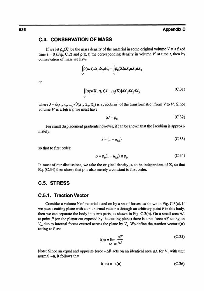
Consider a volume V of material acted on by a set of forces, as shown in Fig. C.3(a).1f we pass a cutting plane with a unit normal vector 0 through an arbitrary point P in this body, then we can separate the body into two parts, as shown in Fig. C.3(b). On a small area M at point P (on the planar cut exposed by the cutting plane) there is a net force ÄF acting on V _ due to internal forces exerted across the plane by V+. We define the traction vector t(o) acting at P as:
t(o) = lim ÄF M-+oM
(C.35)
Note: Since an equal and opposite force -ÄF acts on an identical area M for V+ with unit normal -0, it follows that:
t(-o) = -t(o) (C.36)
Basic Notation and Concepts
(a)
Fig. C.3. (a) A body acted on by external forces and (b) the internal (distributed) forces acting from one part of the body on the adjacent part.
This isjust a statement ofNewton's third law.
C.5.2. Concept of Stress
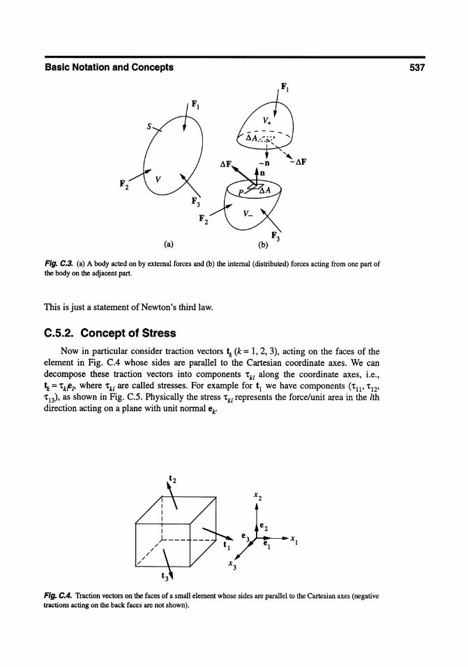
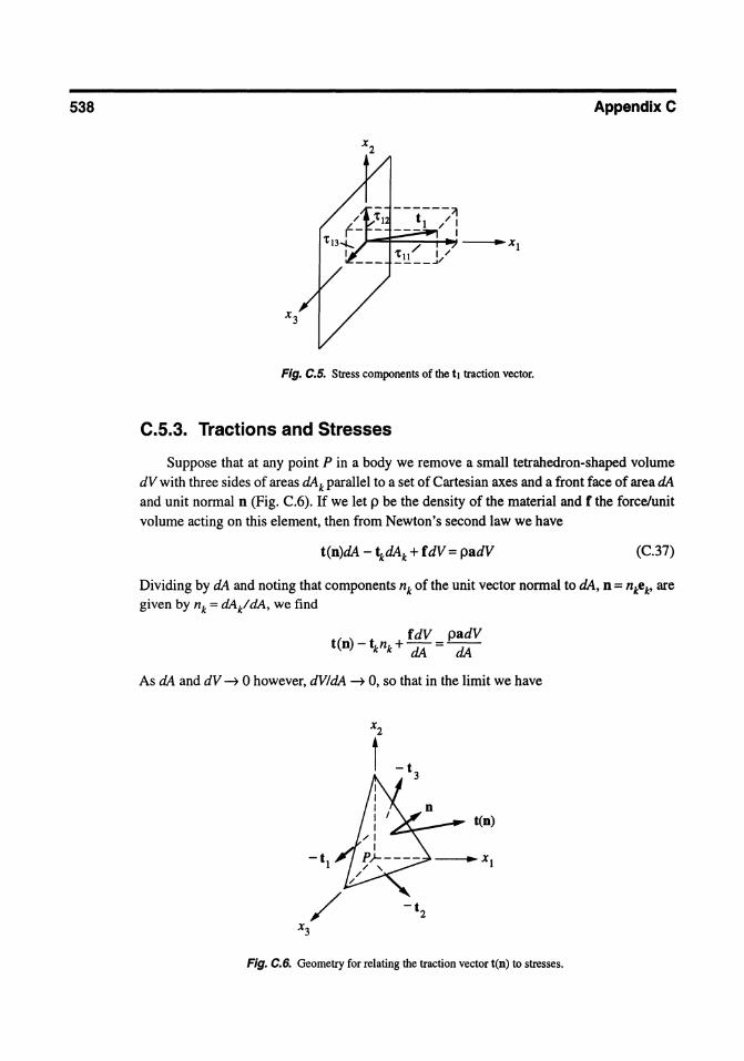
Now in particular consider traction vectors tk (k = 1, 2, 3), acting on the faces of the element in Fig. C.4 whose sides are parallel to the Cartesian coordinate axes. We can decompose these traction vectors into components t k1 along the coordinate axes, Le., tk = tkFl' where t k1 are called stresses. For example for tl we have components (tll , t 12,
t I3), as shown in Fig. C.5. Physically the stress t k1 represents the force/unit area in the lth direction acting on aplane with unit normal ek"
Fig. C.4. Traction vectors on the faces of a small element whose sides are parallel to the Cartesian axes (negative tractions acting on the back faces are not shown).
537
538 Appendix C
------" t l /:
J-.:::j::::::::::;:::::+-'~ - Xl
Fig. C.5. Stress components of the t1 traction vector.
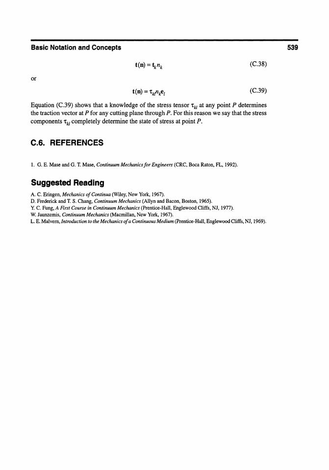
C.5.3. Tractions and Stresses
Suppose that at any point P in a body we remove a small tetrahedron-shaped volume dV with three sides of areas dAk parallel to a set of Cartesian axes and a front face of area dA
and unit normal n (Fig. C.6). If we let p be the density of the material and f the forcelunit
volume acting on this element, then from Newton's second law we have
t(n)dA - tkdAk + f dV = padV (C.37)
Dividing by dA and noting that components n k of the unit vector normal to dA, n = nkek, are given by nk = dAkl dA, we find
As dA and dV ~ ° however, dVldA ~ 0, so that in the limit we have
Fig. C.6. Geometry for relating the traction vector t(n) to stresses.
Basic Notation and Concepts
(C.38)
or
(C.39)
Equation (C.39) shows that a knowledge of the stress tensor 'tkl at any point P determines the traction vector at P for any cutting plane through P. For this reason we say that the stress components 'tkl completely determine the state of stress at point P.
C.6. REFERENCES
1. G. E. Mase and G. T. Mase, Continuum Mechanicsfor Engineers (CRC, Boca Raton, FL, 1992).
Suggested Reading A. C. Eringen, Mechanics ofContinua (Wiley, New York, 1967). D. Frederick and T. S. Chang, Continuum Mechanics (Allyn and Bacon, Boston, 1965). Y. C. Fung, A First Course in Continuum Mechanics (Prentice-Hall, Englewood Cliffs, NJ, 1977). W. Jaunzemis, Continuum Mechanies (Macmillan, New York, 1967). L. E. Malvern, lntroduction to the Mechanies of a Continuous Medium (Prentice-Hall, Englewood Cliffs, NJ, 1969).
539

APPENDIXD
HILBERTTRANSFORM
The Hilbert transform of a functionJtt), which often occurs in signal processing applications and in reflection and refraction problems when critical angles are exceeded, as seen in chapter 6, is defined as [D.I]:
f<>o
I f J(t)dt J~u)=H[f(t);u]=- -
1t t- u
where the integral is interpreted in the principal value sense, i.e.,
(D.!)
(D.2)
As with the Fourier transform, there is an inverse Hilbert transform that can recoverJtt) given by
f<>o
I f J~u)du J(t) =--
1t U - t
0.1. PROPERTIES OF THE HILBERT TRANSFORM
Some of the important properties of the Hilbert transform are given by:
• H[J(a + t); u] = H[J(t); u + a]
• H[f(at); u] = H[f(t); au] (a > 0)
• H[J(-at); u] = H[f(t); -au] (a > 0)
(D.3)
(D.4a)
(D.4b)
(D.4c)
541

542 dfJ..u)
• H[f'(t); u] =----au 1+00
• H[tf(t); u] = ufJ..u) + - J f(t)dt 1t
Appendix 0
(D.4d)
(D.4e)
Hilbert transforms for some commonly occurring functions fit) are shown in the following table.
f(t) H[f{t); u]
B(t) 7tU
H(t - to) -(~}nlu - tol
H(t- b) - H(t- a) (~}nl:=:1 t1>- IH(t) { (-u)1>-1 -<>O<u<o
O<Reu< 1 u1>-lctg(7tU) O<u<oo
sin(aW)H(t) a>O {exp( -a..fit) -<>o<u<O cos(",,") O<u<oo
cos(oot) 00>0 -sin(rou)
sin(oot) 00>0 cos(oou)
Re(a»O a
F+a2 u2 +a2
a u F +a2
Re(a»O - u2 +uZ
0.2. References
1. I. H. Sneddon, Use 01 Integral Trans/orms (McGraw-HilI, New York, 1972).
APPENDIXE
STATIONARY PHASE METHOD
In wave propagation and scattering models, obtaining explicit analytic results is made difficult in many cases by complex interactions. Usually expressions can be reduced only to the form of integrals; these must then be evaluated numerically or approximately. Appendix E considers an approximation method that is particularly useful: The stationary phase method. Basically the method relies on the fact that at high frequencies when the phase term in an integrand varies rapidly, only certain regions contribute significantly to the integral. Assuming high frequencies is a relatively mild assumption in many NDE problems, since characteristic lengths involved in most applications are many wavelengths long. Thus the stationary phase method can often be applied without placing severe restrietions on the validity of results.
E.1. SINGLE-INTEGRAL FORMS
Consider the case of a one-dimensional integral of the form:
b
1= f j(x)exp[ik<j>(x)]dx a
(E.I)
where the wave number k is assumed to be large andj(x) is a smoothly varying function. Since the phase of the complex exponential varies rapidly in this case, with each half-period oscillation nearly canceling the adjacent half-period oscillation of opposite sign, we expect that I ~ 0 as k ~ 00. Under such circumstances the major contribution of the integral comes from points where the phase term <j>(x) is stationary, i.e., <j>'(x) = d<j>/dx = o. To see this consider the following integral:
4
f x( 4 - x)exp[ ik(x - 2)2]dx o
543

544 Appendix E
Figures E.I (a), (b) show the behavior of the real part of this integrand for k = 20 and k = 40, respectively. We see from the behavior of the integrand that most oscillations are canceling except near x = 2, which is a stationary point for the phase term <\lex) == (x - 2f
Assume now that the integral in Eq. (E.!) has one stationary point within the open interval (a, b) at the point Xs where <\l'(xs) == O. Expanding the phase <\lex) in a Taylor series about this point gives
(E.2)
where <\l"(xs) == d2<\l/ tJx2 and s == x - Xs and we assumed <\l"(xs) :t:. O. Since! is assumed to be slowly varying, it is nearly a constant, and it can be removed from the integrand with the constant phase part of the exponential; the major contribution of the remaining integrand comes from the region (xs - c, Xs + c) about the stationary phase point. Thus we have approximately:
s=+E
1== !(xs)exp[ik<\l(xs)] f exp [ik<\l"(xs)s2/2] ds (E.3)
s=-E
However because of the highly oscillatory constant amplitude nature of the integrand in Bq. (E.3), we can replace upper and lower limits by +00 and _00 without introducing significant error to obtain
4
4
· 4
Ca)
·4
(b)
Fig. E.1. The functionx(4 -x) cos[k(x - 2)2] plotted for (a) k = 20, (b) k = 40.

Stationary Phase Method
+00
l = j(x)exp[ik<j>(xs)] f exp[ik<j>"(xs)i l2]ds (EA)
If we let kl<j>"(xs)ls212 = fl, it follows that ds = [2/kl<j>"(xs)l] 1 12dt and the stationary phase approximation of the integralls is
(E.5)
The integral in Eq. (E.5) can be performed exactly, since we have1
+00
f cos(fl)dt = ..Jnl2
+00
f sin(fl)dt = ..Jnl2 (E.6)
so that
+00
f exp[iflsgn{ <j>"(xs)} ]dt = [1 + isgn{ <j>"(xs)} ]..Jnl2
= "I'nexp[insgn{ <j>"(xs)} /4] (E.7)
The integral finally becomes
(E.8)
Equation (E.8) gives an explicit expression for the stationary phase evaluation of the original integral when a single, isolated stationary phase point exists in the open interval (a, b). Special cases when multiple stationary phase points exist, stationary phase point(s) are at the interval end points, and <j>" = 0 at the stationary point can all be considered (see [E.2] for further details). However for specific problems covered in this book, Eq. (E.8) generally suffices.
One special case not covered by Eq. (E.8) we do need to consider is when there is no stationary phase point at all in the closed interval [a, b]. Then we can write l in the form:
b
l = {[ i{<j>~~) 1 [exp{ik<j>(x) }ik<j>'(x)dx] (E.9)
where the second term in square brackets in Eq. (E.9) is a perfect differential, so that integration by parts gives
545
546 Appendix E
b
I=f(x)exp[ikq,(x)] Ib _-!- f [f(x)/q,'(x)]'exp[ikq,(x)]dx (E.lO) ikq,'(x) a Ik
a
Since q,'(x) ":# 0 in [a, b] we can again write the integral in Eq. (E.1O) as the product of two terms, one a perfect differential, then perform the integration by parts again. Thus keeping only the first terms, for k large we have
I =f(b)exp(ikb) f(a)exp(ika) + 0 (1-) ikq,'(b) ikq,'(a) JC2
(E.ll)
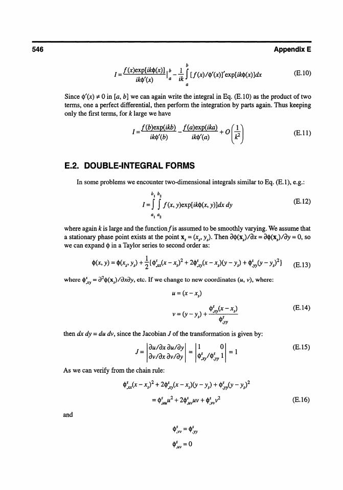
E.2. DOUBLE-INTEGRAL FORMS
In some problems we encounter two-dimensional integrals sirnilar to Eq. (E.l), e.g.:
b1 bz
1= f f f(x, y)exp[ikq,(x, y)]dx dy (E.12)
where again k is large and the functionfis assumed to be smoothly varying. We assume that a stationary phase point exists at the point Xs = (xs' Ys). Then oq,(xs)/ox = oq,(xs)/oy = 0, so we can expand q, in a Taylor series to second order as:
where <!>~ = a2<!>(xs)/axay, etc. If we change to new coordinates (u, v), where:
u = (x -xs)
then dx dy = du dv, since the Jacobian J of the transformation is given by:
J -I ou/ox ou/oy 1_11 0 1- I - ov/ox ov/oy - q,~/q,~yy I -
As we can verify from the chain rule:
q,~(x - xl + 2q,~(x - xs)(y - Ys) + q,~yy(y - yl
= ",s u2 + 2"'s uv + ",s v2 '+',UU 'I',uv 't',vv
and
q,s = 0 .uv
(E.14)
(E.15)
(E.16)
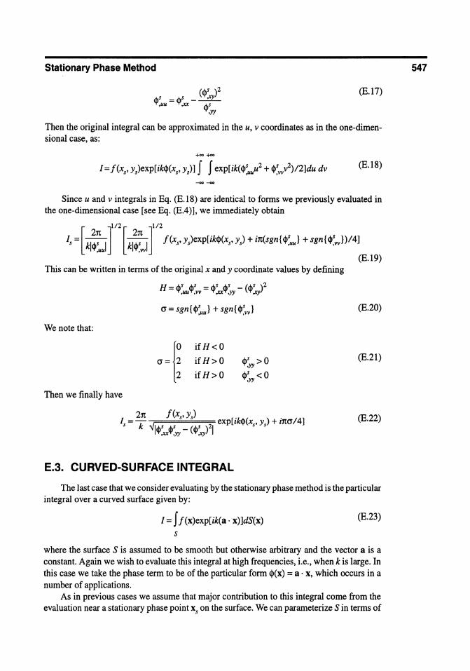
Stationary Phase Method
,j"s =,j"S _ (<jl~l 'I',uu 'I' ,xx ~s
,yy
(E.17)
Then the original integral can be approximated in the u, v coordinates as in the one-dimensional case, as:
+00 too
1= f(xs' y.)exp[ik~(xs' ys)] f f exp[ik(~~uuu2 + ~~wv2)/2]du dv (E.IS)
Since u and v integrals in Eq. (E.IS) are identical to forms we previously evaluated in the one-dimensional case [see Eq. (E.4)], we immediately obtain
1/2 1/2
Is = [kl!~ull [kl!;wll f(xs' y.)exp[ik~(xs' ys) + in(sgn{ ~~uu} + sgn{ ~~w})/4] (E.19)
This can be written in terms of the original x and y coordinate values by defining
We note that:
Then we finally have
H = ~s ~s = ~s ~s _ W )2 ,uu ,w ,xx ,yy ,xy
ifH <0
if H>O
ifH>O
~s > 0 ,yy ~s <0 ,yy
2n f(xs' y.) . . Is = -k " exp[lk<jl(xs' ys) + lncr/4] W ~s -w )21 ,xx ,yy ,xy
E.3. CURVED-SURFACE INTEGRAL
(E.20)
(E.21)
(E.22)
The last case that we consider evaluating by the stationary phase method is the particular integral over a curved surface given by:
1= f f(x)exp[ik(a· x)]dS(x) s
(E.23)
where the surface S is assumed to be smooth but otherwise arbitrary and the vector a is a constant. Again we wish to evaluate this integral at high frequencies, i.e., when k is large. In this case we take the phase term to be of the particular form ~(x) = a . x, which occurs in a number of applications.
As in previous cases we assume that major contribution to this integral come from the evaluation near a stationary phase point Xs on the surface. We can parameterize S in terms of
547
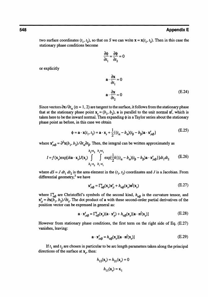
548 Appendix E
two surface coordinates (ti' t2), so that on S we can write x = x(ti' t2). Then in this case the stationary phase conditions become
or explicitly
ax 8·-=0
atl
ax a·-=O
at2
(E.24)
Since vectors ax/ata (a. = 1, 2) are tangent to the surface, it follows from the stationary phase that at the stationary phase point Xs = (bi' b2), a is parallel to the unit normal rI, which is taken here to be the inward normal. Then expanding <1> in a Taylor series about the stationary phase point as before, in this case we obtain
1 <1> = a· x(ti' t2) = 8' Xs + '2{ (ta - bJ(t~ - b~8' ~a~}
(E.25)
where ~aß = a2x(bi' b2)/ataat~. Then, the integral can be written approximately as
b2+E2 bl+EI
1= f(xs)exp[ika· xs]J(xs) f f exp[~k{(ta - bJ(t~ - b~)a' ~aß} ]dtldt2 (E.26)
b2-E2 bi-EI
where dS = J dt l dt2 is the area element in the (ti' t2) coordinates and J is a Jacobian. From differential geometry,3 we have
(E.27)
where ["faß are Christoffel's symbols of the second kind, ha~ is the curvature tensor, and ~y = aX(b l , b2)/aty' The dot product of a with these second-order partial derivatives of the position vector can be expressed in general as:
(E.28)
However from stationary phase conditions, the first term on the right side of Eq. (E.27) vanishes, leaving:
(E.29)
If tl and t2 are chosen in particular to be arc length parameters taken along the principal directions of the surface at xs' then:
Stationary Phase Method
(E.30)
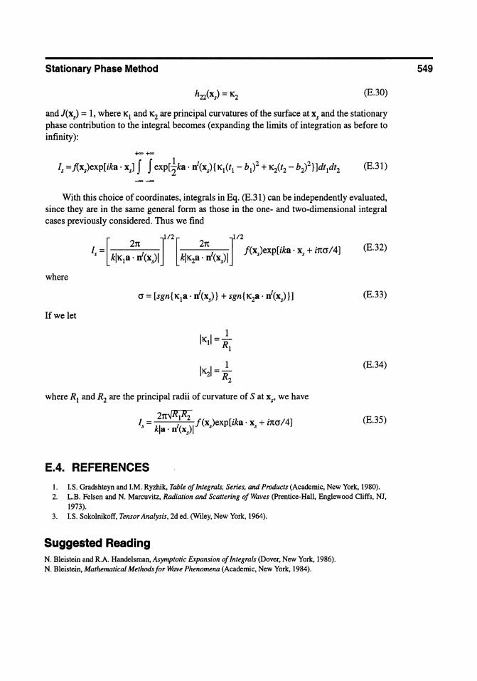
and J(xs) = 1, where K1 and 1S are principal curvatures of the surface at Xs and the stationary phase contribution to the integral becomes (expanding the limits of integration as before to infinity): --
ls = j(xs)exp[ika· xJ f f exp[tka . n1(xs){K1(tl - bi + 1S(t2 - b2)2}]dt1dt2 (E.31)
With this choice of coordinates, integrals in Eq. (E.3l) can be independently evaluated, since they are in the same general form as those in the one- and two-dimensional integral cases previously considered. Thus we find
where
Ifwe let
1 IK21="R
2
where R1 and R2 are the principal radii of curvature of S at xs' we have
21t..jlfTz . . ls = I I I j(x.)exp[zka· Xs + mo/4]
ka· n(xs)
E.4. REFERENCES
(E.32)
(E.33)
(E.34)
(E.35)
1. I.S. Gradshteyn and I.M. Ryzhik, Table of Integrals, Series, and Products (Academic, New York, 1980). 2. L.B. Felsen and N. Marcuvitz, Radiation and Scattering ofWaves (Prentice-Hall, Englewood Cliffs, NI,
1973). 3. I.S. Sokolnikoff, Tensor Analysis, 2d ed. (Wiley, New York, 1964).
Suggested Reading N. Bleistein and R.A. Handelsman, Asymptotic Expansion of Integrals (Dover, New York, 1986). N. Bleistein, Mathematical Methodsfor Wave Phenomena (Academic, New York, 1984).
549

APPENDIXF
PROPERTIES OF ELLIPSOIDS
F.1. GEOMETRV OF AN ELLIPSOID
In Chap. 10, we saw that the far-field scattering response of ellipsoidal inclusions and elliptical cracks can be obtained explicitly through the Born and Kirchhoff approximations. These same approximations are used in Chap. 15 to develop a number of equivalent flaw-sizing algorithms. In Appendix F, we derive some geometrical properties of ellipsoids that are useful in such applications.
One geometrical quantity that frequently appears in Chaps. 10 and 15 is the effective radius re, of an ellipsoid which is the perpendicular distance from the center of an ellipsoid to aplane P that is tangent to its surface at some point xo, as shown in Fig. F.l. If we write the equation of the ellipsoid as:
(F.l)
then since the unit outward normal n is given by n = V g /IV gl, its components are
Fig. F.1. Geometry of an ellipsoid and a plane P tangent to the ellipsoid at point xo. The effective radius re is the distance from the center of the ellipsoid to the plane P in the ei direction, where ei is normal to that plane. 551

552
with
X2 n =-2 Ha2
2
Appendix F
(F.2)
(F.3)
If a plane P, whose unit normal is ei touches and is tangent to the ellipsoid at the point XO = (x~, x~, x~), then ei coincides with the unit normal at this point, i.e., ei = n(x~, x~, x~) = nO, so for any point X in this plane we may write
nO·X=, e (F.4)
which is the general equation for a plane whose unit normal is n° = (n~, n~, n~ and whose perpendicular distance from the origin is the effective radius 'e. Since point XO = (x~, x~, x~ also lies in the plane P, for this point Eq. (F.4) gives
(F.5)
Or from Eqs. (F.I) and (F.2):
(F.6)
Then 'e is given by:
1 1 'e = -EI' = -;=(x=~=)2=/(=a=i)=+=(x=g=)2=/=(a=~)=+=(=XO=3)=2 /=(a=~::')
(F.7)
To obtain a more useful form for 'e' consider expression ai(n?)2 + a~(n~2 + ai(n~2. From Eqs. (F.1), (F.2), and (F.7):
ai(n~)2 + a~(ng)2 + a~(n~)2
(x~)2 / ai + (xg)2 / a~ + (~)2 / a~ =
(EI')2
=,2 e (F.8) Then we finally have
'e = ai(n~)2 + a~(ng)2 + a~(n~)2
= 1 aI(ei · ul + a~(ei . Üz)2 + a~(ei . ui (F.9)
where (ul' u2, u3) are unit vectors along the axes of the ellipsoid (Fig. F.1). Thus if we are given the normal to the plane ei and the size and orientation of the ellipsoid through parameters (al' a2, a3) and (ul' u2, u3), respectively, Eq. (F.9) determines the effective radius. Also the point where the plane touches the ellipsoid can then be obtained, since:

Properties of Ellipsoids
(F.1O)
Note: Equations (F.2), (F.4), and (F.6) also imply that an equivalent form for the plane P is given by:
(F.U)
which is a commonly derived result in differential geometry texts. As shown in Chap. 15 measuring an effective radius of an unknown flaw from different
directions allows us to use Eq. (F.9) to obtain the equivalent ellipsoidal size and orientation parameters for that flaw. Thus Eq. (F.9) is the key geometric relationship for performing equivalent flaw sizing.
Another geometrical parameter of interest (see the leading edge response of ellipsoids in Chap. 10) is the Gaussian curvature of the ellipsoid. To obtain an expression for this curvature, we parameterize the surface of the ellipsoid by two parameters (tl' t2) as follows:
(F.12)
Then any point x on the ellipsoid is given by:
x = aicosticost2u I + a2costisint2Uz + a3sint2~ (F.13)
From differential geometry the mean and Gaussian curvatures M and K, respectively, of a surface are given by:1
where gaß and haß are the first and second fundamental forms:
gaß = x'a' x'ß
ha~ = nI . x'a~
(F.14)
(F.15)
553
554 Appendix F
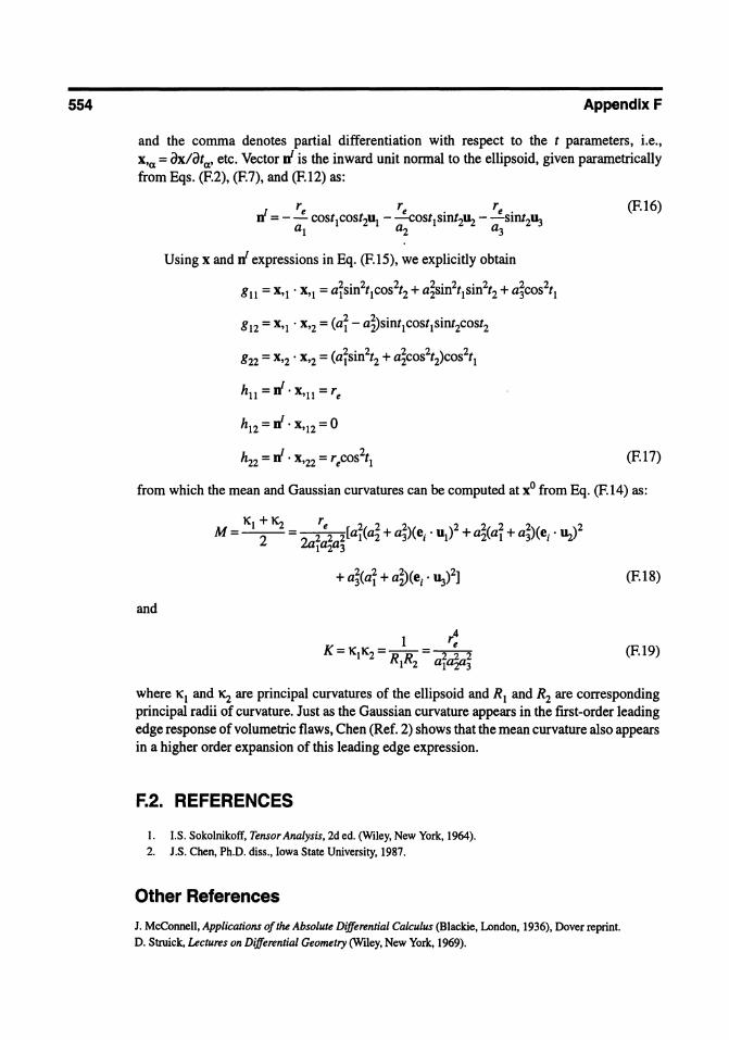
and the comma denotes partial differentiation with respect to the t parameters, i.e., x'a = ox/ota, etc. Vector .r is the inward unit normal to the ellipsoid, given parametrically from Eqs. (F.2), (F.7), and (F.12) as:
Using x and.r expressions in Eq. (F.15), we explicitly obtain
2·222'2·222 g11 = X'I . X'I = alsm tlcos t2 + a2sm tlsm t2 + a3cos tl
(F.16)
(F.17)
from which the mean and Gaussian curvatures can be computed at XO from Eq. (F.14) as:
(F.18)
and
(F.19)
where KI and ~ are principal curvatures of the ellipsoid and R I and R2 are corresponding principal radii of curvature. Just as the Gaussian curvature appears in the first-order leading edge response of volumetric flaws, ehen (Ref. 2) shows that the mean curvature also appears in a higher order expansion of this leading edge expression.
F.2. REFERENCES
1. I.S. Sokolnikoff, Tensor Analysis, 2d ed. (Wiley, New York, 1964). 2. J.S. Chen, Ph.D. diss., Iowa S1a1e University, 1987.
Other References
J. McConnell, Applications ofthe Absolute Differential Calculus (Blackie, London, 1936), Dover reprint. D. Struick, Lectures on Differential Geometry (Wiley, New York, 1969).
INDEX
Absorption losses, 284 Acoustic emission, 12 Acoustic impedance, 93
table of values, 41 Acoustic intensity
for a fluid, 94, 95 for an elastic solid, 120, 121
Acoustic lens: see Spherically focused transducer in a fluid
Aliasing, 521 Almanski strain tensor, 534 Alternating tensor, 530 ALOK,509 Angle beam shear wave transducer, 125,419-424 Angular spectrum of plane waves, 60, 179, 200, 260 Antiplane strain: see Goveming equations, elastic
solid Area function: see Flaw area function and impulse
response for scattering A-scan,l1 Associated Legendre functions, 364 Attenuation term in the LTI model, 297
Beam diameter, focused probe: see Focal spot size Beam models numerical evaluation, 244 Born approximation
for a fluid, 328-332 for an elastic solid, 352-356
Boundary diffraction wave theory, 178-181 Boundary elements, 76, 82 B-scan, 11 Bulk modulus, 30, 40 Bulk waves, 39-40
Cartesian tensor notation: see Indicial notation Cauchy strain tensor, 534
Caustics, 231, 238 Characteristic function, 500 Christoffel symbol, 548 Circular frequency, 17 Constitutive equations
for an elastic solid, 35-36 for a fluid, 30
Contact transducer for P-waves, 6 for S-waves, 6
Convolution, 16, 25 and Fourier Transforms, 20
Couplant,6 Crack width function for scattering
in a fluid, 327-328 in asolid, 349-352
Critical angle(s), 99, 118 Cross correlation, 24 C-scan,11
D' Alembert solution, 67 Damping setting, 3 Dead region, 8 Decibel, 285 Deconvolution, 295-296,481-483 Delay line contact transducer, 8 Depth of focus, 279 Diffraction correction
defined, 164 term in the LTI model, 275
Diffraction correction integral, 289-295 Digitizer, 9-10 Dilatation, 30, 40 Dirac delta function, 19,527-528
in three dimensions, 57 Direct waves, 160 555
556
Directivity functions, 266 Discrete delta function, 523, 525 Dispersion
geometrieal, 148 material, 287
Divergence theorem, 533
Edge elements for an angle beam shear wave transducer model,
272-275 for a curved interface
fluid-fluid problem, 256-258 fluid-solid problem, 258-260
defined,246-247 for a focused probe, 247-251 for a fluid-solid interface, 253-256
Edge waves, 160 Effective focallength, 461 Effective radius
for an ellipsoidal flaw, 316, 551-552 for an elliptical crack, 324 for a focused transducer, 460 for a planar transducer, 458-460
Efficiency factor, 23, 288 determination by deconvolution, 298-301 term in the LTI model, 300
EFIT,487 Elastic constant tensor, 36
for an isotropie material, 36 Electromechanical reciprocity: see Reciprocal
theorem Ellipsoid
Gaussian curvature, 554 mean curvature, 554
Energy flux for an elastic solid, 119-121 for a fluid, 94
Equations of motion for a fluid, 29 for asolid, 33
Equivalent flaw sizing, 491 Equivalent radius: see Effective radius Equivalent-time samp1ing, 9 Euler's theorem, 227 Extensional waves: see Plate waves
Far-field scattering amplitude: see Scattering amplitude
Far-field scattering amplitude integrals for volumetrie flaws
in a fluid, 306, 331, 354 in asolid, 308-310
for cracklike flaws in a fluid, 307 in asolid, 311
Far-field scattering amplitude integrals (cant.) for volumetrie flaws in two-dimensions
in a fluid, 381 in asolid, 382
Fast Fourier transform (FFT), 18,524 Fermat's principle, 115 Finite-part integral, 82 Flash points, 167, 326, 492 Flat-bottom hole models
fluid-fluid,476 fluid-solid,469-475
Index
Flaw area function and impulse response for scattering in a fluid, 319-320, 335-336 in asolid, 357
Flaw scattering amplitude term in the LTI model, 377 Flaw sizing: see Born flaw sizing; Kirchhoff flaw
sizing; TOPE flaw sizing Flexural waves: see Plate waves Focal spot size, 197, 279 Focused transducer models: see Transducer radiation
models (focused transducer) Fourier transform, 16,517-519 Fraunhofer approximation, 251-253 Fundamental solution
for a fluid, 57, 59 forms in the far field
for a fluid, 61 for asolid, 66
integral forms, 59 for asolid, 62
Gauss function, 26, 519 Gaussian curvature, 553; see also Ellipsoid Gauss-Hermite beam model, 244-245 Gauss' theorem. 532-533 Generalized Snell's law: see Snell's law Governing equations, elastic solid
antiplane strain conditions, 45 displacement formulation, 41-43 plane strain conditions, 44-45 potential formulation, 43-44
Grain scattering, 284 Group velocity, 154
Hankelfunction, 382 Harmonie waves, 51 Heaviside step function, 519, 528 Helmholtz decomposition, 39 Helmholtz equation, 59 Hessian, 263, 547 Hilbert transform, 103,541-542 Hyperelastic material, 35 Hypersingular integral equation, 82
Impedance: see Acoustic impedance
Index
Impedance boundary condition, 380 Immersion testing, 6 Impulse response function, 19,20 Impulse response method, 486 Indicial notation, 529-532 Inhomogeneous waves, 99,118 Integral equations
for a fluid, 75-77 for asolid, 81-82
Integral forms of the fundamental solution: see Fundamental solution
Integral representation theorem for a fluid, 70-72 for asolid, 78-79
Intensity: see Acoustic intensity Interfacelboundary conditions
for a fluid, 32 for asolid, 37
Inverse Fourier transform, 16, 517
Jacobian, 536, 548
Kirchhoff approximation for propagation through a curved interface, 223 for the scattering amplitude (fluid-cracks),
322-323 for the scattering amplitude (fluid-volumetrie
flaws),312-314 for the scattering amplitude ( solid-cracks),
344-346 for the scattering amplitude (solid-volumetrie
flaw),336-341 Kirchhoffflaw sizing, 491-493 Kronecker delta function, 530
Lamb waves: see Plate waves (extensional and flexural modes)
Lame constants, 36 Lame's theorem, 47 Leading edge response for a volumetrie flaw
defined,318 in a fluid, 320-322 in asolid, 341-344
Legrendre polynomials, 365 Lens: see Acoustic lens Linear least squaresleigenvalue sizing, 494-498 Love wave, 153 Linear-time-shift invariant systems, 15 Linearity, 16 LTI measurement models: see also Reciprocity-based
measurement models for a fluid-fluid interface, 404 for a fluid-solid interface, 405-407 for a single fluid medium, 399-403
Mass conservation, 536 Maxwell's equations, 83 Mean curvature, 553 see also Ellipsoid Measurement models: see LTI measurement models;
Reciprocity-based measurement models; Near-field measurement models
Mode of a plate wave: see Plate waves Mode conversion, 115 Moment theorem, 25 MOOT,483,485
Navier's equations, 36 Near-field measurement models
for an on-axis spherical scatterer in a fluid, 441-443
for an on-axis cylindrical scatterer in a fluid, 443-446
for a planar transducer at normal incidence to a fluid-solid interface, 451-454
for a single fluid medium (general scatterer) pressure-pressure model, 449 pressure-velocity model, 449 velocity-pressure model, 435-440 velocity-velocity model, 449
in the paraxial approximation limit, 446 Near-field distance, 162 Non-linear least squares sizing, 493 Numerical evaluation ofbeam models: see Beam
models numerical evaluation NURBS,484 Nyquist criterion, 521
O'Neil model, 181-183
Paraxial approximation, 164 Parseval's theorem, 24 Piezoelectric medium reciprocal theorem: see
Reciprocal theorem Piston model of a transducer, 158 Pitch-catch setup, 10 Planar aperture model- focused transducer, 182-183,
189 Planar piston transducer in a fluid
boundary diffraction waves, 171-174 diffraction corrections, 164, 168-171 far field response, 163 impulse response, 175-178 off-axis response, 165-165 on-axis response, 160-163
Planar transducer models: see Transducer radiation models (planar transducer)
Plane of incidence, 110 Plane strain: see Goveming equations, elastic solid Planewaves
in a fluid (one-dimensional), 49-52
557
558
Plane waves (cant.) in a fluid (three-dimensional), 52 in asolid (one-dimensional), 53 in asolid (three-dimensional), 53-56
Plate waves, 46 for extensional modes, 150 for flexural modes, 152 forSHmodes, 145-149
Poisson's ratio, 36 Polarization, 55
on reception, 391-392 Potentials
for elastic waves, 39 in plane wave amplitudes, 55
Pressure-pressure model: see Near-field measurement models
Pressure-velocity model: see Near-field measurement models
Principal curvatures, 549 Principal value integral, 75 Prob ability of detection, 403, 486 Propagation term in the LTI model, 66 Pulse distortion, 102, 119,349-350 Pulse-echo setup, 10 Pulser-receiver, 1, 3
Quarter wave plate, 8, 138
Radiation conditions: see Sommerfeld radiation conditions
Ramp response, 505 Rayleigh-Sommerfeld theory, 158-160 Rayleigh's theorem: see Parseval's theorem Rayleigh wave, 8,141-145 Real-time sampling, 9 Reception process model
for a fluid-fluid interface, 387-390 for a fluid-solid interface, 391-394 for a single fluid, 385-387
Reception term in the LTI model, 394 Reciprocal theorem
for an electromechanical (piezoelectric) system, 83
for a fluid, 69, 359 in one-dimension, 86 for asolid, 77, 360
Reciprocity-based measurement models: see also LTI measurement models for angle beam shear wave inspection, 419-424 for contact inspection (electromechanical
model), 424-427 for a general immersion setup, 407-415 reduced to an LTI model, 415-419
Reciprocity of scattering amplitudes in a fluid, 357-360
Reciprocity of scattering amplitudes (cant.) in asolid, 360-361
Reflection coefficients for a fluid-fluid interface, 97-100 for a fluid-solid interface, 115-119
Index
at a free surface of an elastic solid, 133-134 for normal incidence, 91-94 for a solid-solid smooth interface, 123-127 for a solid-solid welded interface, 127-132
Rod waves, 46 Rodrigues' formula, 365 Rotation, 40, 535
SAFT,509 Satellite pulse method, 508-509 Scattering amplitude integrals: see Far field scattering
amplitude integrals Scattering amplitude
deterrnined experimentally, 481-483 for an ellipsoid (fluid), 314-318 for an elliptical crack (fluid), 323-327 for an elliptical crack (solid), 346-348
Separation of variables for a spherical fluid inclusion in asolid, 376 for a spherical inclusion in asolid, 374-375 for a spherical scatterer in a fluid, 362-367 for a spherical void, 375
SH-waves, 53, 55 Sign function, 99, 519 Simulation, ultrasonic, 484-486 Sizing: see Flaw sizing Snell's law, 98
generalized, 116 and stationary phase, 112
Sommerfeld integral, 61 Sommerfeld radiation conditions
for a fluid, 72 in one-dimension, 86 for asolid, 79 in two-dimensions, 87
Spherical Bessel functions, 363 Spherical Hankelfunctions, 363 Spherical waves: see Fundamental solution Spherically focused transducer in a fluid
diffraction corrections, 187-188, 192 exact model - direct and edge waves, 193-197 focusing by an acoustic lens, 197-199 limitations of diffraction corrections, 193 off-axis response, 189-192 on-axis response, 183-187 planar aperture model: see Planar aperture
model - focused transducer Stationary phase method
for a double integral, 546-547 for a single integral, 543-546

Index
Stationary phase method (cont.) for a surface integral, 547-549
Strain tensor: see Almanski strain tensor, Cauchy strain tensor
Stokes' relations for a fluid-fluid interface, 106 for a fluid-solid interface, 122-123
Stokes' theorem, 533 Stoneley wave, 153 Stress tensor, 35, 537-539 SV-waves, 53, 55 Surface wave: see Rayleigh wave System efficiency factor: see Efficiency factor
Time-shift invariance, 16 Through-transmission setup, 10 TOFE flaw sizing, 505-508 TOFD method, 508 Total reflection, 101 Traction vector, 536 Transducers
for angle beam shear wave testing, 8 for contact testing, 5-6 for immersion testing, 7-8
Transducer characterization: see Effective radius; Effective focallength
Transducer radiation models (planar transducer) curved interface
fluid-fluid, 221-237 fluid-solid, 238-243
plane fluid-fluid interface (normal incidence), 199-205
plane fluid-fluid interface (oblique incidence), 209-214
plane fluid-solid interface (normal incidence), 206-208
plane fluid-solid interface (oblique incidence), 214-215
single fluid: see Planar piston transducer in a fluid
Transducer radiation models (focused transducer) curved interface
fluid-fluid, 221-231, 237-238 fluid-solid, 238-244
plane fluid-fluid interface, 215-219
Transducer radiation models (focused transducer) (cont.) plane fluid-solid interface, 219-221 single fluid: see Spherically focused transducer
in a fluid Transfer matrix, 136 Transmission coefficients
for a fluid-fluid interface, 97-100 for a fluid-solid interface, 115-119 for normal incidence, 91-94 for a solid-solid smooth interface, 123-127 for a solid-solid welded interface, 127-132
Transmission terms in the LTI model, 134
Ultrasonic simulation: see Simulation, ultrasonic Unit impulse response function, 19 Unit step function: see Heaviside step function
Velocity, see Wave speed Velocity, group: see Group velocity Velocity-pressure model: see Near-field measurement
models Velocity-velocity model: see Near-field measurement
models
Wave equation for a fluid, 31 for asolid, 39-40, 53
Wave number, 51 Wave speed
of pressure waves in a fluid, 32 of P-waves, 39 of Rayleigh waves, 143 of S-waves, 39 of SH plate waves, 147 table of values, 41
Wavelength, 51 Wear plate, 5 Weyl's integral, 60 Width function: see Crack width function for
scattering Wiener filter, 296, 463, 482 Work-kinetic energy theorem, 47
Young's modulus, 36
Zero-of-time problem, 505
559