Embed Size (px)
Citation preview

11/2/2009
1
Chapter 4Image Enhancement in the
Frequency Domain
Chapter 4Image Enhancement in the
Frequency Domain
Fourier TransformFrequency Domain Filtering
Low-pass, High-pass, Butterworth, GaussianLaplacian, High-boost, Homomorphic
Properties of FT and DFTTransforms
4.1
Transforms
Chapter 4Image Enhancement in the
Frequency Domain
Chapter 4Image Enhancement in the
Frequency Domain
4.2

11/2/2009
2
Chapter 4Image Enhancement in the
Frequency Domain
Chapter 4Image Enhancement in the
Frequency Domain
u
4.3
Chapter 4Image Enhancement in the
Frequency Domain
Chapter 4Image Enhancement in the
Frequency Domain
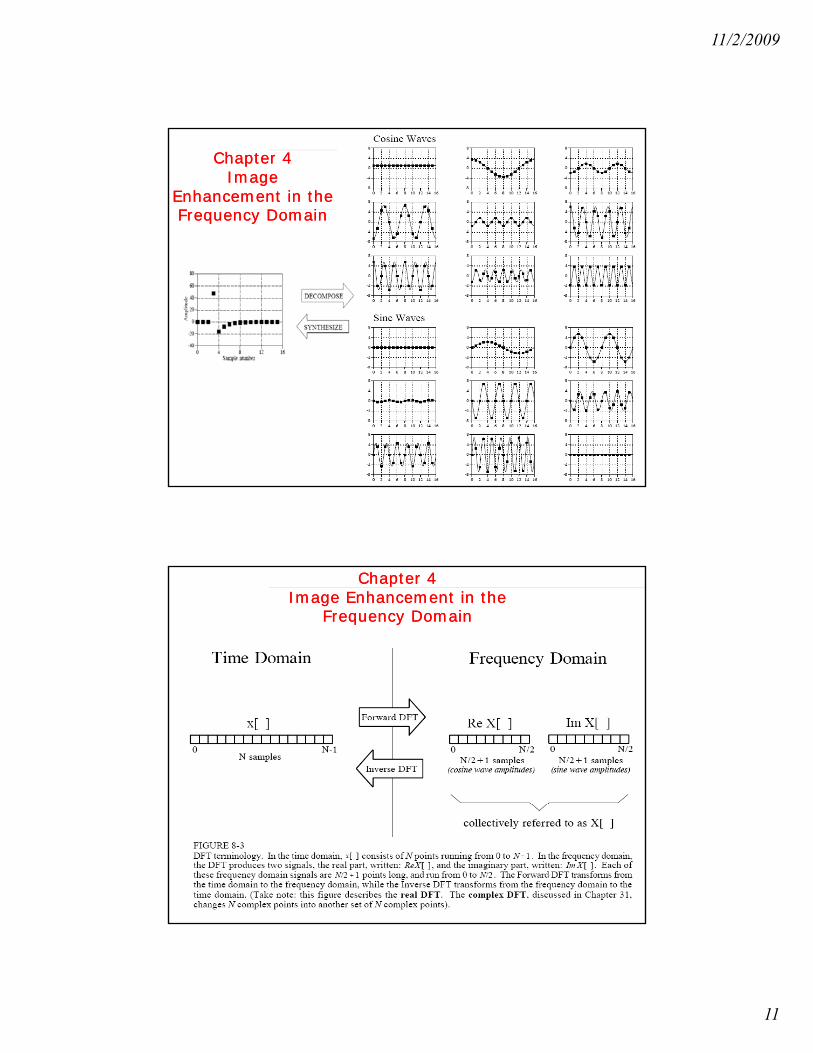
Fourier, 1807Fourier series states that a periodicfunction can be represented by a weighted sum of sinusoids
,
+
=
4.4
Periodic and non-periodicfunctions can be representedby an integral of weightedsinusoids
=

11/2/2009
3
Chapter 4Image Enhancement in the
Frequency Domain
Chapter 4Image Enhancement in the
Frequency Domain
4.5
Chapter 4Image
Enhancement in theFrequency Domain
Chapter 4Image
Enhancement in theFrequency Domain
4.6

11/2/2009
4
Chapter 4Image Enhancement in the
Frequency Domain
Chapter 4Image Enhancement in the
Frequency Domain
4.7
Chapter 4Image Enhancement in the
Frequency Domain
Chapter 4Image Enhancement in the
Frequency Domain
4.8

11/2/2009
5
Chapter 4Image Enhancement in the
Frequency Domain
Chapter 4Image Enhancement in the
Frequency Domain
4.9
Chapter 4Image Enhancement in the
Frequency Domain
Chapter 4Image Enhancement in the
Frequency Domain
4.10

11/2/2009
6
Chapter 4Image Enhancement in the
Frequency Domain
Chapter 4Image Enhancement in the
Frequency Domain
4.11
4.12
11/2/2009
7
Chapter 4Image Enhancement in the
Frequency Domain
Chapter 4Image Enhancement in the
Frequency Domain
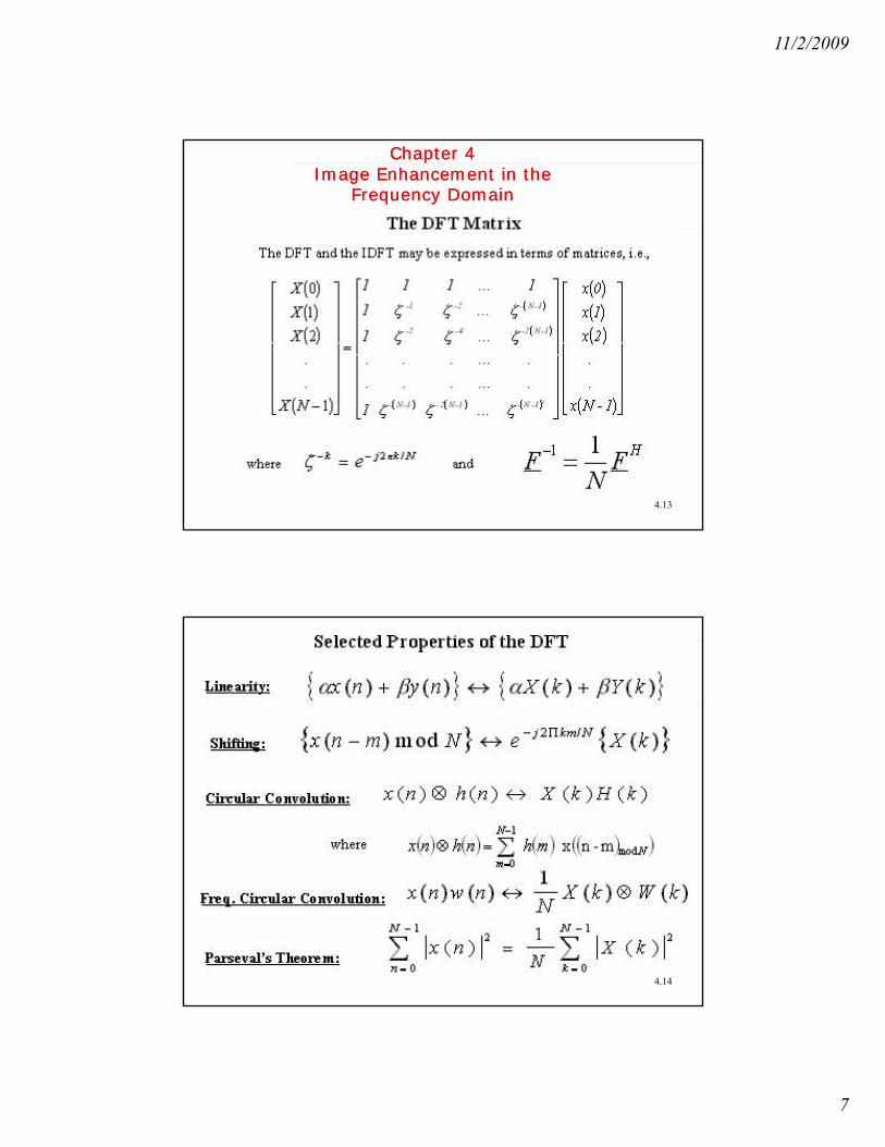
4.13
4.14
11/2/2009
8
Chapter 4Image Enhancement in the
Frequency Domain
Chapter 4Image Enhancement in the
Frequency Domain
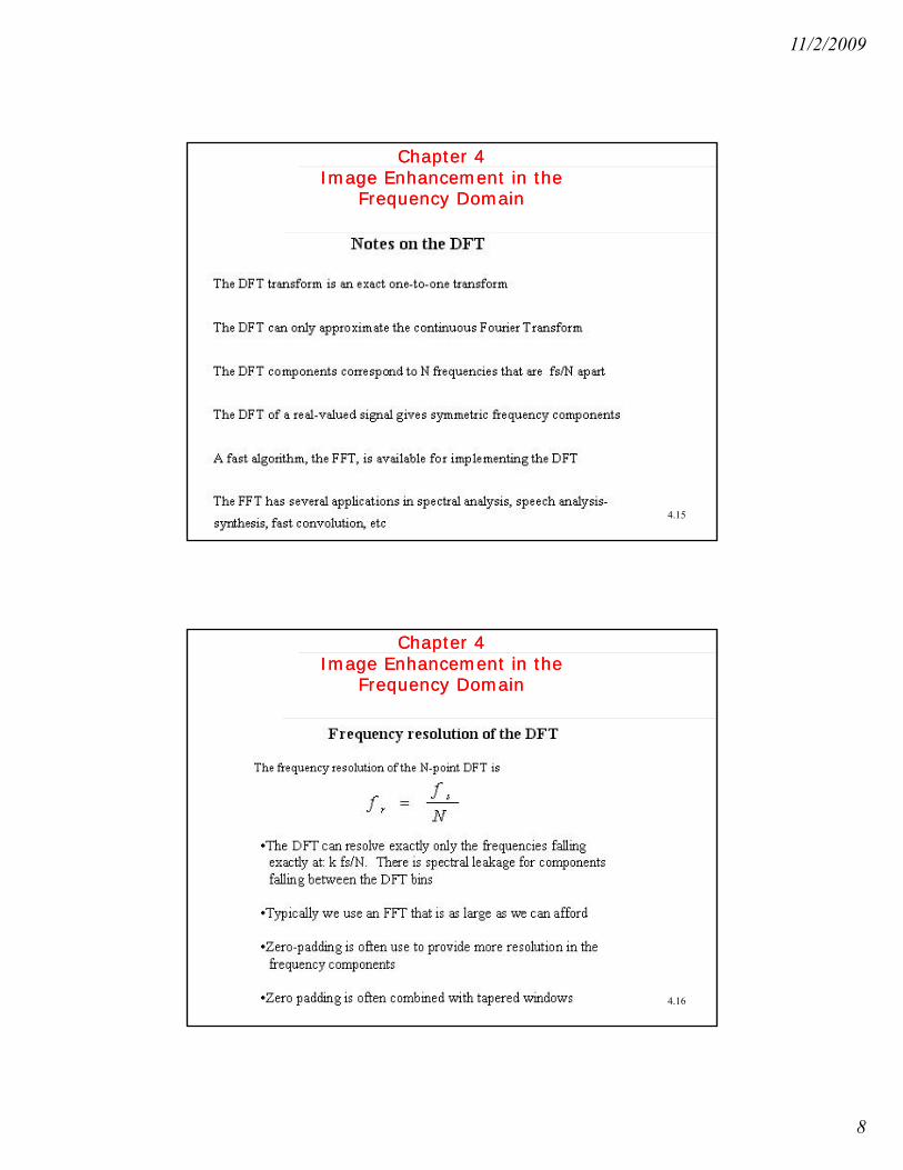
4.15
Chapter 4Image Enhancement in the
Frequency Domain
Chapter 4Image Enhancement in the
Frequency Domain
4.16
11/2/2009
9
Chapter 4Image Enhancement in the
Frequency Domain
Chapter 4Image Enhancement in the
Frequency Domain
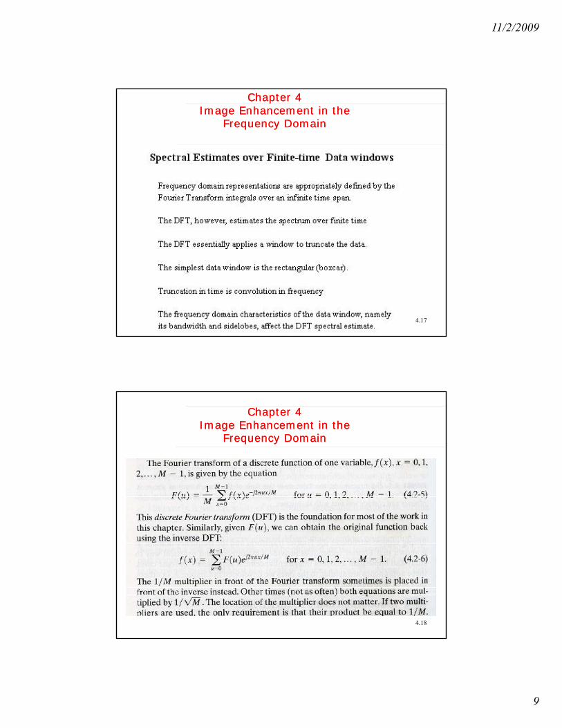
4.17
Chapter 4Image Enhancement in the
Frequency Domain
Chapter 4Image Enhancement in the
Frequency Domain
4.18
11/2/2009
10
Chapter 4Image Enhancement in the
Frequency Domain
Chapter 4Image Enhancement in the
Frequency Domain
4.19
Chapter 4Image Enhancement in the
Frequency Domain
Chapter 4Image Enhancement in the
Frequency Domain
4.20
∑ ∑= =
+=2/
0
2/
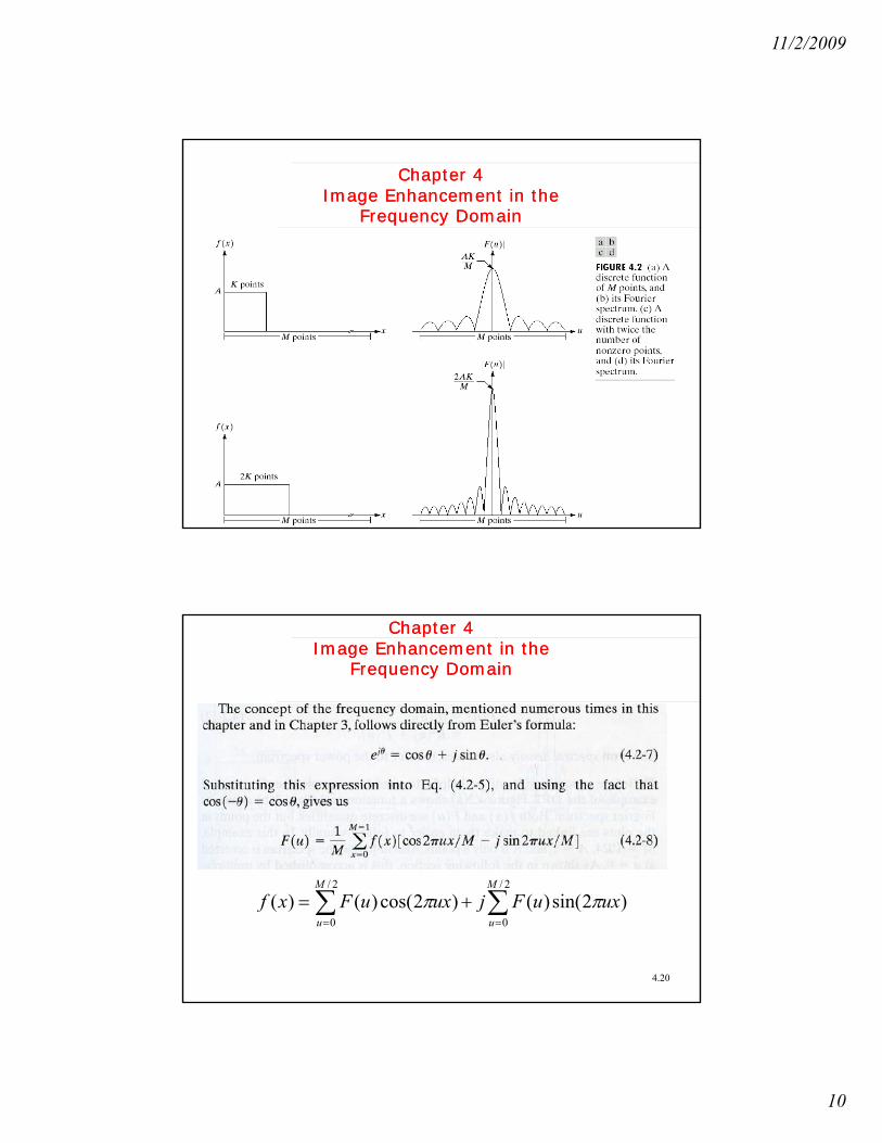
0)2sin()()2cos()()(
M
u
M
uuxuFjuxuFxf ππ
11/2/2009
11
Chapter 4Image
Enhancement in theFrequency Domain
Chapter 4Image
Enhancement in theFrequency Domain
4.21
Chapter 4Image Enhancement in the
Frequency Domain
Chapter 4Image Enhancement in the
Frequency Domain
4.22

11/2/2009
12
Chapter 4Image Enhancement in the
Frequency Domain
Chapter 4Image Enhancement in the
Frequency Domain
4.23
Chapter 4Image Enhancement in the
Frequency Domain
Chapter 4Image Enhancement in the
Frequency Domain
4.24

11/2/2009
13
Chapter 4Image Enhancement in the
Frequency Domain
Chapter 4Image Enhancement in the
Frequency Domain
4.25
Chapter 4Image Enhancement in the
Frequency Domain
Chapter 4Image Enhancement in the
Frequency Domain
4.26
11/2/2009
14
Chapter 4Image Enhancement in the
Frequency Domain
Chapter 4Image Enhancement in the
Frequency Domain
4.27
Chapter 4Image Enhancement in the
Frequency Domain
Chapter 4Image Enhancement in the
Frequency Domain
4.28
11/2/2009
15
Chapter 4Image Enhancement in the
Frequency Domain
Chapter 4Image Enhancement in the
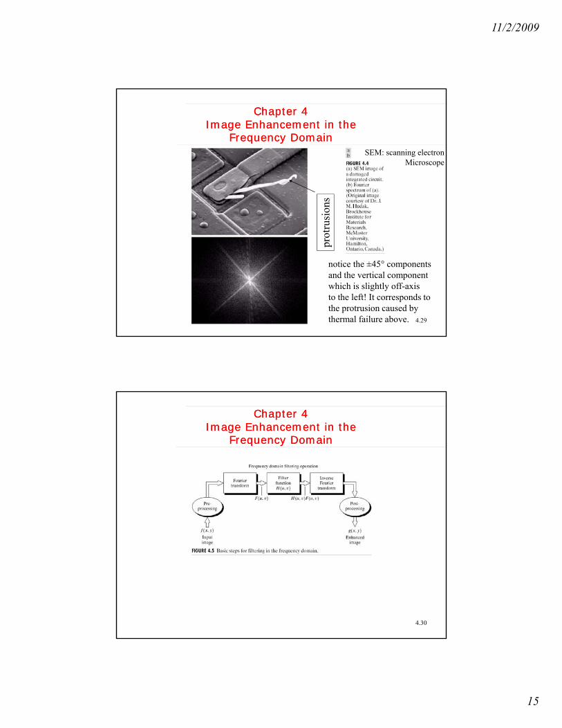
Frequency DomainSEM: scanning electron
Microscope
prot
rusi
ons
4.29
notice the ±45° componentsand the vertical componentwhich is slightly off-axisto the left! It corresponds tothe protrusion caused by thermal failure above.
Chapter 4Image Enhancement in the
Frequency Domain
Chapter 4Image Enhancement in the
Frequency Domain
4.30

11/2/2009
16
Chapter 4Image Enhancement in the
Frequency Domain
Chapter 4Image Enhancement in the
Frequency Domain
Basic Filtering Examples:1 Removal of image average1. Removal of image average
• in time domain?• in frequency domain:• the output is: ⎩
⎨⎧ =
=otherwise
NMvuifvuH
1)2/,2/(),(0
),(
),(),(),( vuFvuHvuG =
This is called the notch filter,i t t f ti ith
4.31
i.e. a constant function witha whole at the origin.
how is this image displayedif the average value is 0?!
Chapter 4Image Enhancement in the
Frequency Domain
Chapter 4Image Enhancement in the
Frequency Domain
2. Linear Filters
2.1. Low-pass
2.2. High-pass
4.32

11/2/2009
17
Chapter 4Image Enhancement in the
Frequency Domain
Chapter 4Image Enhancement in the
Frequency Domain
another result of high-pass g pfiltering where a constant has been addedto the filter so as it will not completely eliminate F(0,0).
4.33
Chapter 4Image Enhancement in the
Frequency Domain
Chapter 4Image Enhancement in the
Frequency Domain
3. Gaussian Filters
frequency domain 22 2/)( σuAeuH −=
22222)( xAexh σπσπ −=
4.34
spatial domain
Low-pass high-pass

11/2/2009
18
Chapter 4Image Enhancement in the
Frequency Domain
Chapter 4Image Enhancement in the
Frequency Domain
4. Ideal low-pass filter⎩⎨⎧ ≤
= 0
)(0
),(1),(
DvuDif
DvuDifvuH
f⎩ 0),(0 DvuDif f
D0 is the cutoff frequency and D(u,v) is the distance between (u,v) and thefrequency origin.
4.35
Chapter 4Image Enhancement in the
Frequency Domain
Chapter 4Image Enhancement in the
Frequency Domain
4.36
• note the concentration of image energy inside the inner circle.• what happens if we low-pass filter it with cut-off freq. at the
position of these circles? (see next slide)
11/2/2009
19
Chapter 4Image Enhancement in the
Frequency Domain
Chapter 4Image Enhancement in the
Frequency Domain
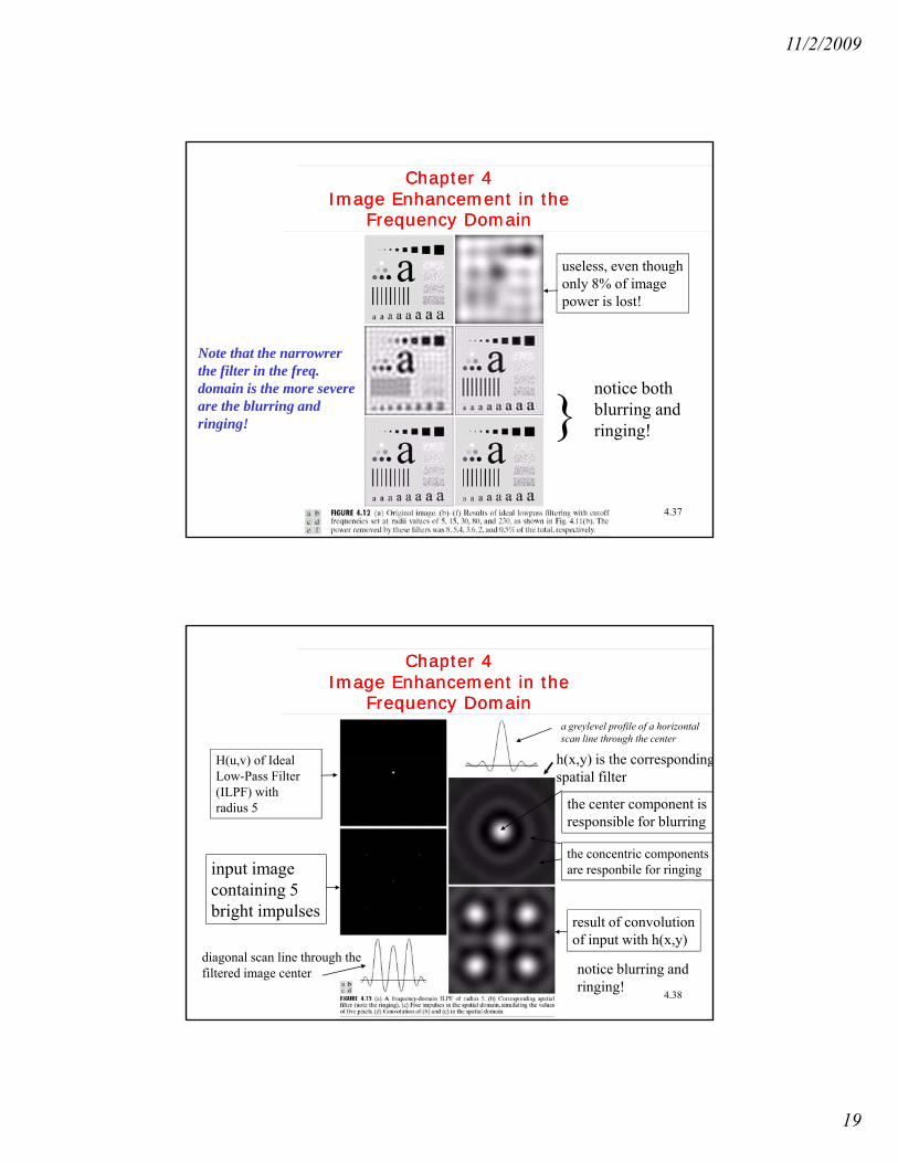
useless, even thoughgonly 8% of imagepower is lost!
}notice bothbl i d
Note that the narrowrerthe filter in the freq. domain is the more severeare the blurring and
4.37
} blurring andringing!
are the blurring and ringing!
Chapter 4Image Enhancement in the
Frequency Domain
Chapter 4Image Enhancement in the
Frequency Domain
H( ) f Id l h( ) i th di
a greylevel profile of a horizontalscan line through the center
H(u,v) of IdealLow-Pass Filter (ILPF) withradius 5
input image containing 5
the center component isresponsible for blurring
the concentric componentsare responbile for ringing
h(x,y) is the correspondingspatial filter
4.38
containing 5bright impulses
result of convolutionof input with h(x,y)
notice blurring andringing!
diagonal scan line through thefiltered image center

11/2/2009
20
Chapter 4Image Enhancement in the
Frequency Domain
Chapter 4Image Enhancement in the
Frequency Domainhow to achieve blurring with little or no ringing? BLPF is one technique
4.39
nDvuDvuH 2
0 ]/),([11),(
+=
Transfer function of a BLPF of order n and cut-off frequencyat distance D0 (at which H(u,v) is at ½ its max value) from the origin:
2/122 ])2/()2/[(),( NvMuvuD −+−=where
D(u,v) is just the distance from point (u,v) to the center of the FT
Chapter 4Image Enhancement in the
Frequency Domain
Chapter 4Image Enhancement in the
Frequency Domain
Filtering with BLPFwith n=2 and increasing note the smooth transition
in blurring achieved as acut-off as was done withthe Ideal LPF
in blurring achieved as a function of increasing cutoffbut no ringing is present in any of the filtered imageswith this particular BLPF (with n=2)
this is attributed to
4.40
this is attributed to the smooth transitionbet low and highfrequencies
11/2/2009
21
Chapter 4Image Enhancement in the
Frequency Domain
Chapter 4Image Enhancement in the
Frequency Domain
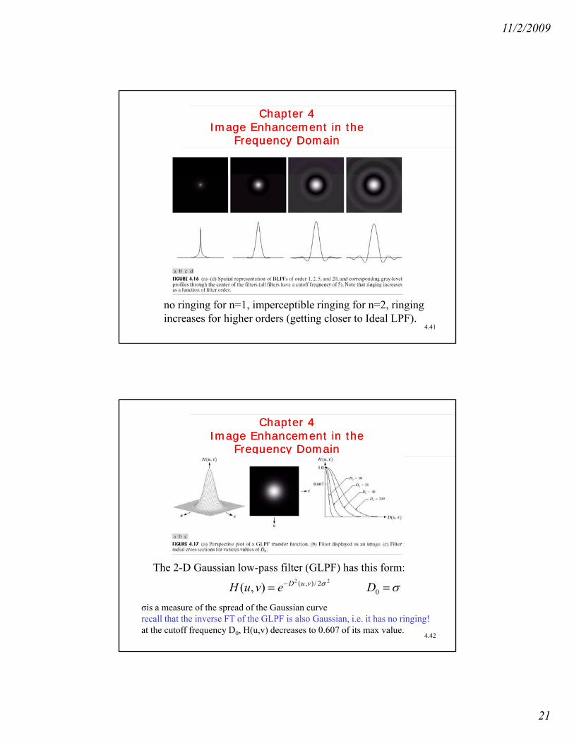
4.41
no ringing for n=1, imperceptible ringing for n=2, ringingincreases for higher orders (getting closer to Ideal LPF).
Chapter 4Image Enhancement in the
Frequency Domain
Chapter 4Image Enhancement in the
Frequency Domain
The 2 D Gaussian low pass filter (GLPF) has this form:
4.42
The 2-D Gaussian low-pass filter (GLPF) has this form:22 2/),(),( σvuDevuH −=
σis a measure of the spread of the Gaussian curverecall that the inverse FT of the GLPF is also Gaussian, i.e. it has no ringing!at the cutoff frequency D0, H(u,v) decreases to 0.607 of its max value.
σ=0D

11/2/2009
22
Chapter 4Image Enhancement in the
Frequency Domain
Chapter 4Image Enhancement in the
Frequency Domain
Results of GLPFs 2 L thi thResults of GLPFs 2. Less smoothing than BLPFs since the latter have tighter control over the transitions bet low and high frequencies.
The price paid for tighter control by using BLP is
Remarks:
1. Note the smooth transition in blurring achieved as a function
4.43
3. No ringing!
y gpossible ringing.of increasing cutoff
frequency.
Chapter 4Image Enhancement in the
Frequency Domain
Chapter 4Image Enhancement in the
Frequency Domain
Applications: fax transmission, duplicated documents and old records.
4.44
GLPF with D0=80 is used.

11/2/2009
23
Chapter 4Image Enhancement in the
Frequency Domain
Chapter 4Image Enhancement in the
Frequency DomainA LPF is also used in printing, e.g. to smooth fine skin lines in faces.
4.45
Chapter 4Image Enhancement in the
Frequency Domain
Chapter 4Image Enhancement in the
Frequency Domain
(a) a very high resolution radiometer (VHRR) image showing part of the Gulf of Mexico (dark) and Florida (light) taken from NOAAthe Gulf of Mexico (dark) and Florida (light) taken from NOAA satellitle. Note horizontal scan lines caused by sensors.
4.46
(b) scan lines are removed in smoothed image by a GLP with D0=30(c) a large lake in southeast Florida is more visible when more agressive smoothing is applied (GLP with D0=10).
11/2/2009
24
Chapter 4Image Enhancement in the Frequency Domain
Sharpening Frequency Domain Filters
Chapter 4Image Enhancement in the Frequency Domain
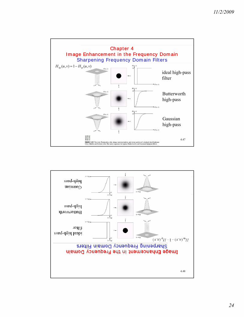
Sharpening Frequency Domain Filters),(1),( vuHvuH lphp −=
ideal high-passg pfilter
Butterworthhigh-pass
4.47
Gaussianhigh-pass
4.48
11/2/2009
25
Chapter 4Image Enhancement in the
Frequency Domain
Chapter 4Image Enhancement in the
Frequency Domain
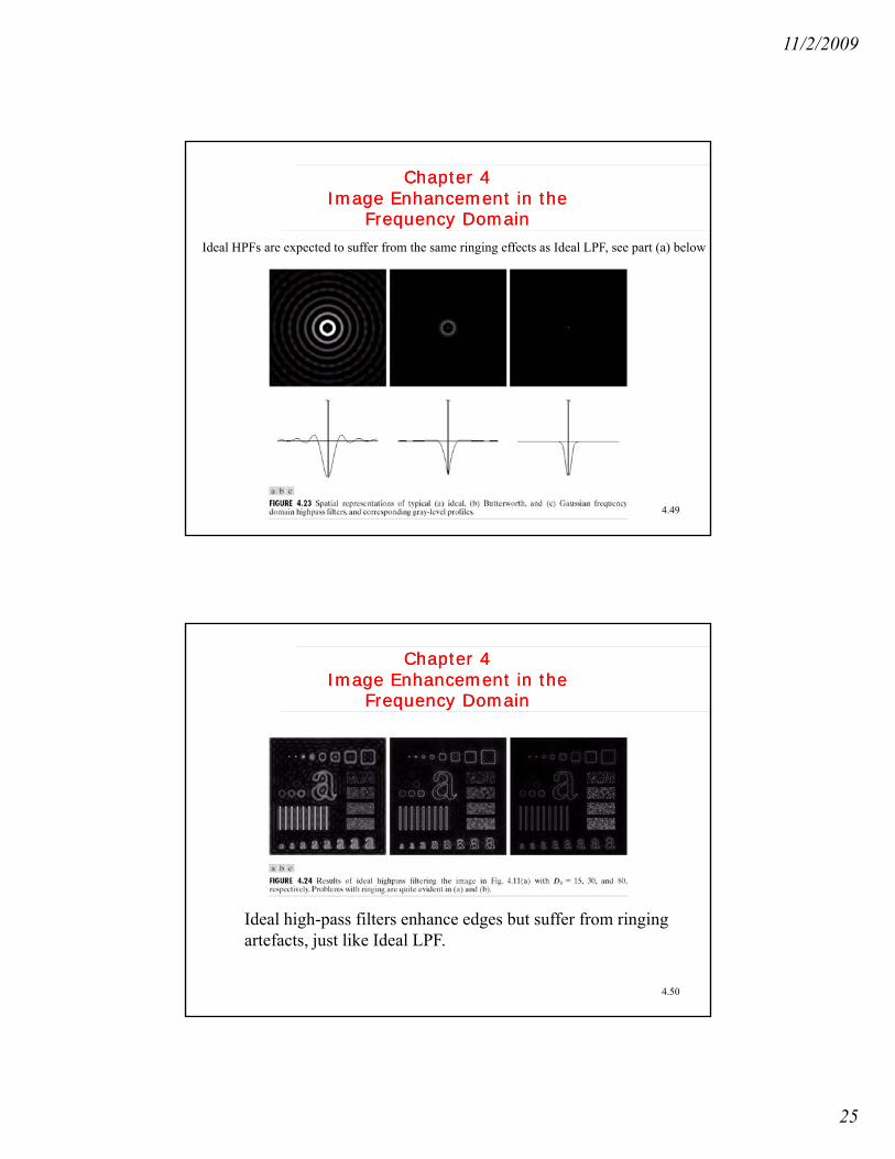
Ideal HPFs are expected to suffer from the same ringing effects as Ideal LPF, see part (a) below
4.49
Chapter 4Image Enhancement in the
Frequency Domain
Chapter 4Image Enhancement in the
Frequency Domain
4.50
Ideal high-pass filters enhance edges but suffer from ringingartefacts, just like Ideal LPF.

11/2/2009
26
Chapter 4Image Enhancement in the
Frequency Domain
Chapter 4Image Enhancement in the
Frequency Domain
4.51
improved enhanced images with BHPFs
Chapter 4Image Enhancement in the
Frequency Domain
Chapter 4Image Enhancement in the
Frequency Domain
4.52
even smoother results with GHPFs

11/2/2009
27
Ideal HPF
BHPF
4.53
GHPF
Chapter 4Image Enhancement in the
Frequency Domain
Chapter 4Image Enhancement in the
Frequency Domain
Laplacian in the frequency domainh th tone can show that:
)()()( uFjudx
xfdFT nn
n
=⎥⎦
⎤⎢⎣
⎡
From this, it follows that:
[ ] ),()(),(),(),( 2222
2
2
2
vuFvuyxfFTy
yxfx
yxfFT +−=∇=⎥⎦
⎤⎢⎣
⎡∂
∂+
∂∂
Th f th L l i b i l t d i f b
4.54
Therefore, the Laplacian can be implemented in frequency by:
)(),( 22 vuvuH +−=
Recall that F(u,v) is centered if [ ]),()1(),( yxfFTvuF yx+−=and thus the center of the filter must be shifted, i.e.
[ ]22 )2/()2/(),( NvMuvuH −+−−=

11/2/2009
28
Chapter 4Image Enhancement in the
Frequency Domain
Chapter 4Image Enhancement in the
Frequency DomainLaplacian in the frequencydomain image representation
H(u,v)of H(u,v)
IDFT of image
close-up of thecenter part
4.55
IDFT of imageof H(u,v) grey-level profile
through the centerof close-up
Chapter 4Image Enhancement in the
Frequency Domain
Chapter 4Image Enhancement in the
Frequency Domain
result of filteringorig in frequencydomain by Laplacian
previous result enhanced result
4.56
previous resultscaled
enhanced resultobtained using
),(),(),( 2 yxfyxfyxg ∇−=
11/2/2009
29
Chapter 4Image Enhancement in the
Frequency Domain: high-boost filtering
Chapter 4Image Enhancement in the
Frequency Domain: high-boost filtering
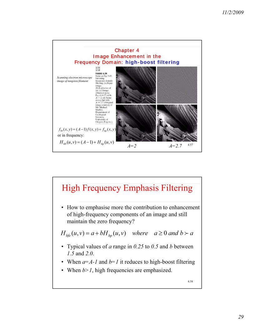
Scanning electron microscopeScanning electron microscopeimage of tungsten filament
4.57
),(),()1(),( yxfyxfAyxf hphb +−=or in frequency:
),()1(),( vuHAvuH hphb +−=A=2 A=2.7
High Frequency Emphasis Filtering
• How to emphasise more the contribution to enhancement of high frequency components of an image and stillof high-frequency components of an image and still maintain the zero frequency?
• Typical values of a range in 0.25 to 0.5 and b between 1 5 d 2 0
abandawherevubHavuH hphfe f0),(),( ≥+=
4.58
1.5 and 2.0. • When a=A-1 and b=1 it reduces to high-boost filtering• When b>1, high frequencies are emphasized.
11/2/2009
30
Chapter 4Image Enhancement in the
Frequency Domain
Chapter 4Image Enhancement in the
Frequency Domain
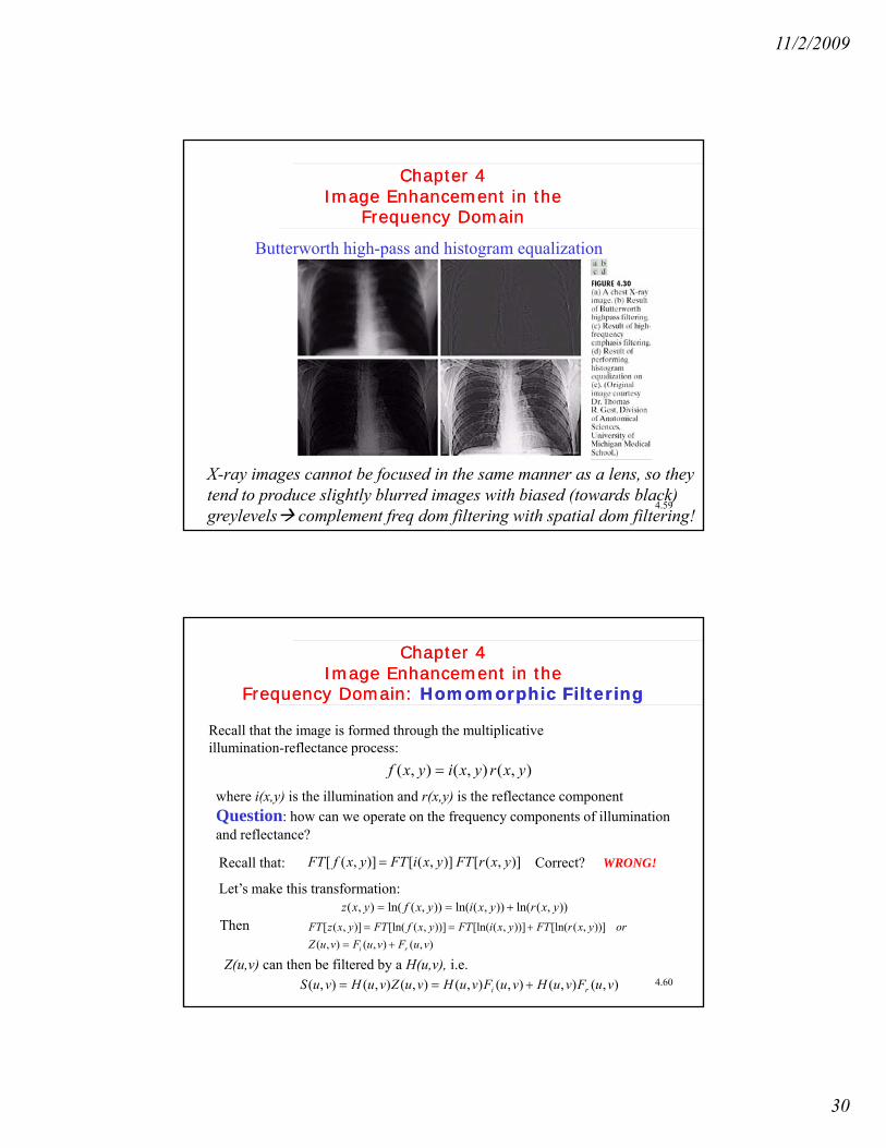
Butterworth high-pass and histogram equalization
4.59
X-ray images cannot be focused in the same manner as a lens, so theytend to produce slightly blurred images with biased (towards black) greylevels complement freq dom filtering with spatial dom filtering!
Chapter 4Image Enhancement in the
Frequency Domain: Homomorphic Filtering
Chapter 4Image Enhancement in the
Frequency Domain: Homomorphic Filtering
Recall that the image is formed through the multiplicativeillumination reflectance process:illumination-reflectance process:
),(),(),( yxryxiyxf =
where i(x,y) is the illumination and r(x,y) is the reflectance componentQuestion: how can we operate on the frequency components of illuminationand reflectance?
Recall that: Correct?)],([)],([)],([ yxrFTyxiFTyxfFT = WRONG!
4.60
Let’s make this transformation:)),(ln()),(ln()),(ln(),( yxryxiyxfyxz +==
Then),(),(),(
))],([ln())],([ln())],([ln()],([vuFvuFvuZ
oryxrFTyxiFTyxfFTyxzFT
ri +=+==
Z(u,v) can then be filtered by a H(u,v), i.e.),(),(),(),(),(),(),( vuFvuHvuFvuHvuZvuHvuS ri +==

11/2/2009
31
Chapter 4Image Enhancement in the
Frequency Domain: Homomorphic Filtering
Chapter 4Image Enhancement in the
Frequency Domain: Homomorphic Filtering
4.61
Chapter 4Image Enhancement in the
Frequency Domain: Homomorphic filtering
Chapter 4Image Enhancement in the
Frequency Domain: Homomorphic filtering
if the gain of H(u,v) is set such as
1pLγ and 1fHγ
then H(u,v) tends to
4.62
( , )decrease the contributionof low-freq (illum) andamplify high freq (refl)
Net result: simultaneous dynamic range compression and contrast enhancement

11/2/2009
32
Chapter 4Image Enhancement in the
Frequency Domain
Chapter 4Image Enhancement in the
Frequency Domain
4.63
5.0=Lγ and 0.2=Hγ
details of objects inside the shelter which were hiddendue to the glare from outside walls are now clearer!
Chapter 4Image Enhancement in the Frequency Domain:
Implementation Issues of the FT: origin shifting
Chapter 4Image Enhancement in the Frequency Domain:
Implementation Issues of the FT: origin shifting
one full periodinside the interval
4.64
11/2/2009
33
Chapter 4Image Enhancement in theFrequency Domain: Scaling
Chapter 4Image Enhancement in theFrequency Domain: Scaling
4.65
Chapter 4Image Enhancement in the
Frequency Domain: Periodicity & Conj. Symmetry
Chapter 4Image Enhancement in the
Frequency Domain: Periodicity & Conj. Symmetry
4.66
11/2/2009
34
Chapter 4Image Enhancement in the
Frequency Domain: separability of 2-D FT
Chapter 4Image Enhancement in the
Frequency Domain: separability of 2-D FT
4.67
Chapter 4Image Enhancement in the
Frequency Domain: Convolution (Wraparound Error)
Chapter 4Image Enhancement in the
Frequency Domain: Convolution (Wraparound Error)
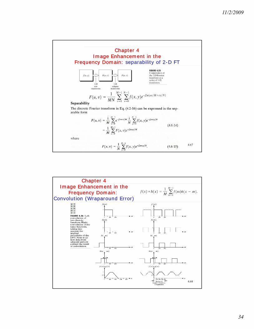
4.68

11/2/2009
35
Chapter 4Image Enhancement in the
Frequency Domain: Convolution (Wraparound Error)
Chapter 4Image Enhancement in the
Frequency Domain: Convolution (Wraparound Error)
4.69
Chapter 4Image Enhancement in the
Frequency Domain: zero-padding in 2D
Chapter 4Image Enhancement in the
Frequency Domain: zero-padding in 2D
4.70

11/2/2009
36
Chapter 4Image Enhancement in the
Frequency Domain: zero padding in convolution
Chapter 4Image Enhancement in the
Frequency Domain: zero padding in convolution
4.71
Chapter 4Image Enhancement in the
Frequency Domain (Convolution & Correlation)
Chapter 4Image Enhancement in the
Frequency Domain (Convolution & Correlation)
4.72
11/2/2009
37
Chapter 4Image Enhancement in the
Frequency Domain (Convolution & Correlation)
Chapter 4Image Enhancement in the
Frequency Domain (Convolution & Correlation)
4.73
Chapter 4Image Enhancement in the
Frequency Domain (Matching Filter)
Chapter 4Image Enhancement in the
Frequency Domain (Matching Filter)
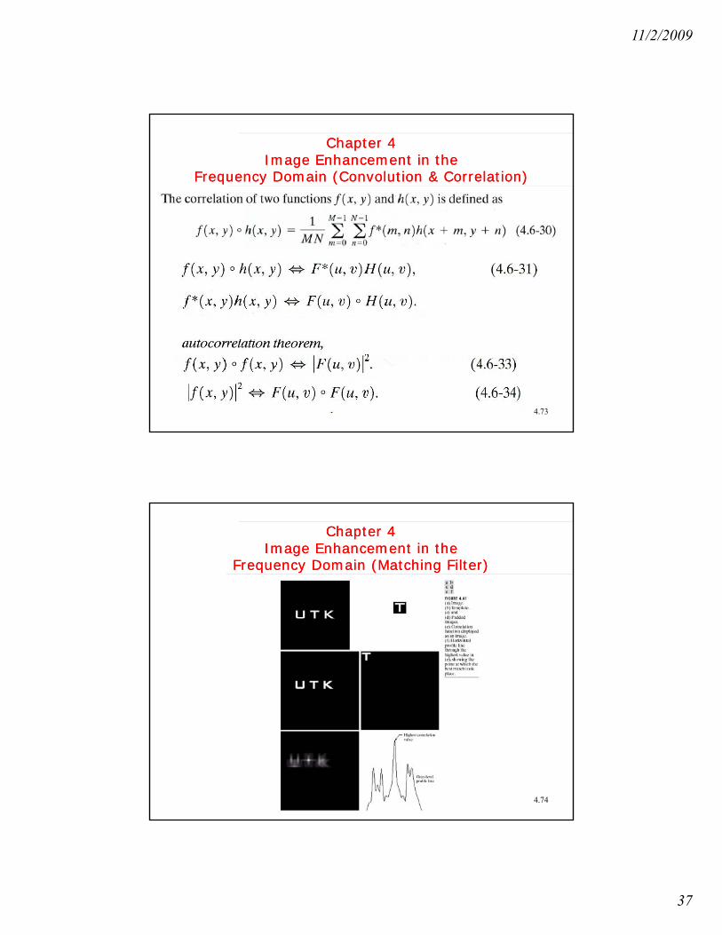
4.74

11/2/2009
38
IntroductionW h ll id i l di i l
Image TransformsImage Transforms
We shall consider mainly two-dimensional transformations.
Transform theory has played an important role in image processing.
4.75
Image transforms are used for image enhancement, restoration, encoding and analysis.
Image Transforms
Examples1. In Fourier Transform, ,
a) the average value (or “d.c.” term) is proportional to the average image amplitude.
b) the high frequency terms give an indication of the amplitude and orientation of image edges.
2. In transform coding, the image bandwidth requirement can be reduced by discarding or coarsely quantizing small coefficients.
4.76
3. Computational complexity can be reduced, e.g.a) perform convolution or compute
autocorrelation functions via DFT,b) perform DFT using FFT.

11/2/2009
39
Image TransformsUnitary TransformsRecall thatRecall that
– a matrix A is orthogonal if A-1=AT
– a matrix is called unitary if A-1=A*T
(A* is the complex conjugate of A).
A unitary transformation:
4.77
A unitary transformation:v=Au,
u=A-1v=A*Tvis a series representation of u where v is the vector of the series
coefficients which can be used in various signal/image processing tasks.
Image Transforms
In image processing, we deal with 2-D transforms.Consider an NxN image u(m n)Consider an NxN image u(m,n).An orthonormal (orthogonal and normalized) series
expansion for image u(m,n) is a pair of transforms of the form:
∑∑−
=
−
=
=1
0
1
0, ),(),(),(
N
m
N
nlk nmanmulkv
4.78
∑∑−
=
−
=
∗=1
0
1
0, ),(),(),(
N
k
N
llk nmalkvnmu
where the image transform {akl(m,n)} is a set of complete orthonormal discrete basis functions satisfying the following two properties:
11/2/2009
40
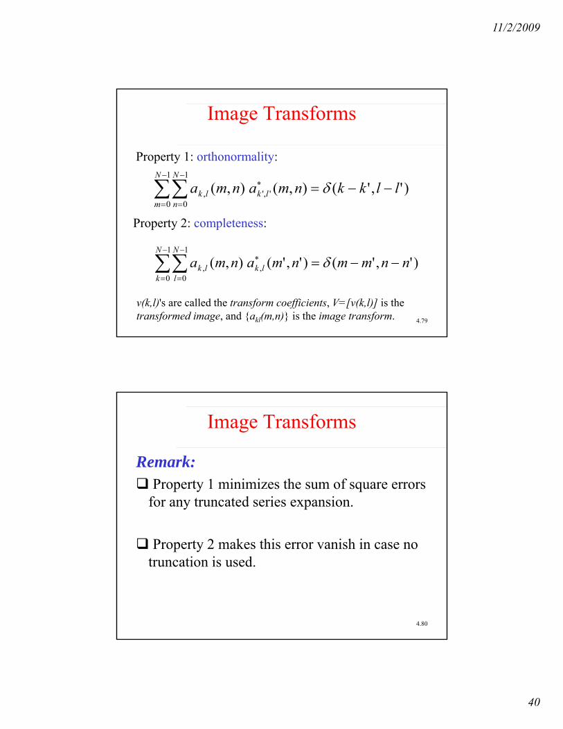
Image Transforms
Property 1: orthonormality:
)','(),(),(1
0
1
0',', llkknmanma
N
m
N
nlklk −−=∑∑
−
=
−
=
∗ δ
Property 2: completeness:
1 1N N− −
4.79
)','()','(),(0 0
,, nnmmnmanmak l
lklk −−=∑∑= =
∗ δ
v(k,l)'s are called the transform coefficients, V=[v(k,l)] is the transformed image, and {akl(m,n)} is the image transform.
Image Transforms
Remark:Property 1 minimizes the sum of square errors
for any truncated series expansion.
Property 2 makes this error vanish in case no i i d
4.80
truncation is used.
11/2/2009
41
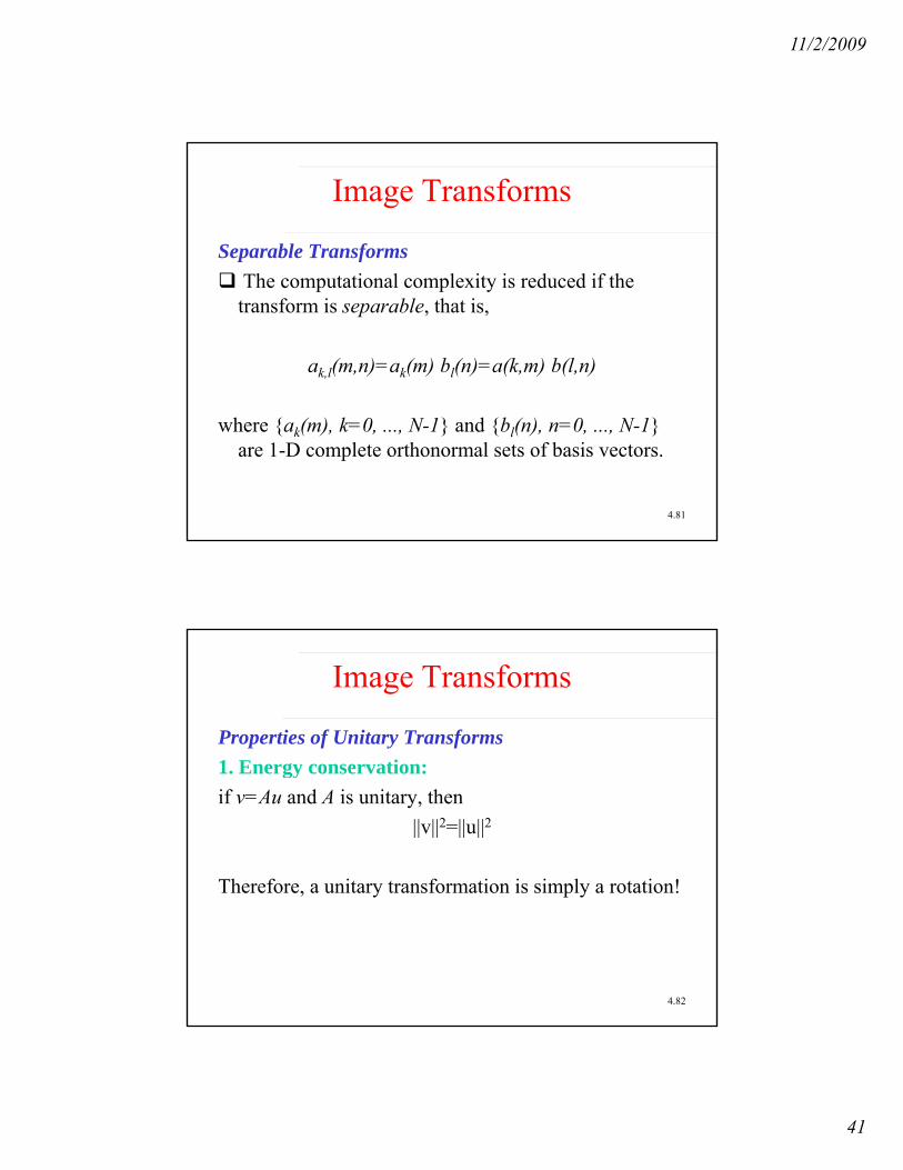
Image Transforms
Separable TransformsTh i l l i i d d if hThe computational complexity is reduced if the transform is separable, that is,
ak,l(m,n)=ak(m) bl(n)=a(k,m) b(l,n)
4.81
where {ak(m), k=0, ..., N-1} and {bl(n), n=0, ..., N-1} are 1-D complete orthonormal sets of basis vectors.
Image Transforms
Properties of Unitary Transforms1 E ti1. Energy conservation: if v=Au and A is unitary, then
||v||2=||u||2
Therefore, a unitary transformation is simply a rotation!
4.82
, y p y
11/2/2009
42
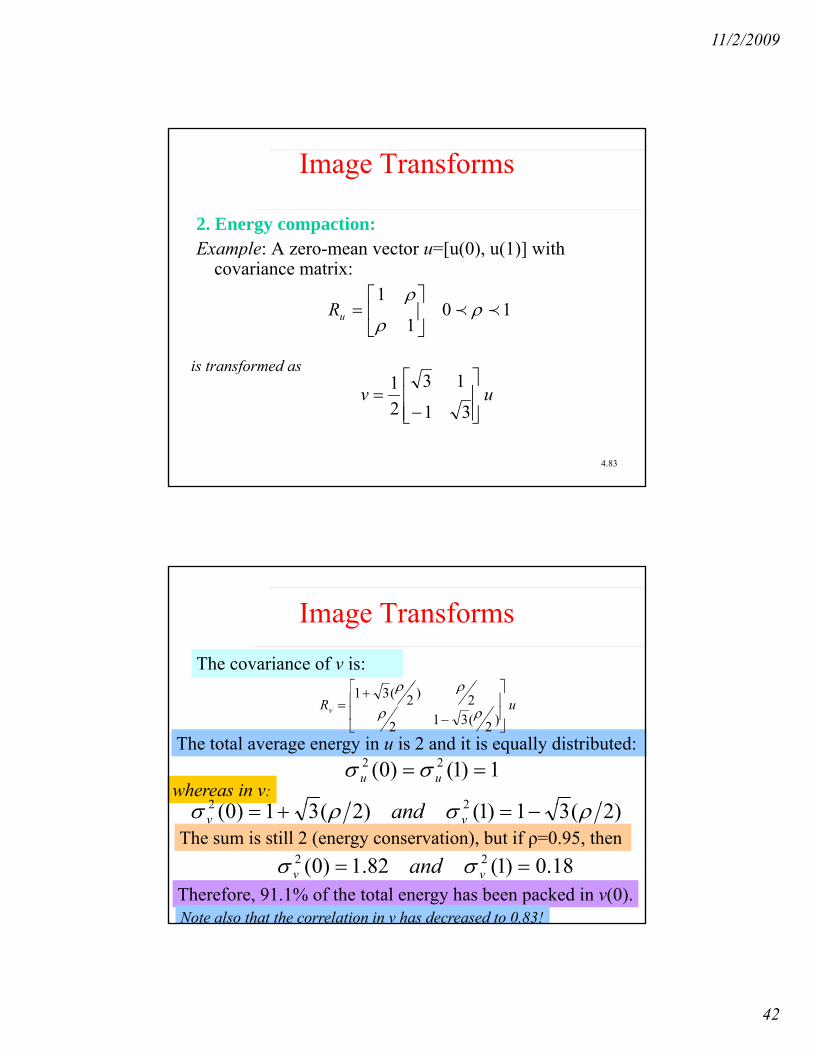
Image Transforms
2. Energy compaction: Example: A zero mean vector u=[u(0) u(1)] withExample: A zero-mean vector u=[u(0), u(1)] with
covariance matrix:
101
1pp ρ
ρ
ρ⎥⎦
⎤⎢⎣
⎡=uR
is transformed as
4.83
is transformed as
uv⎥⎥⎦
⎤
⎢⎢⎣
⎡
−=
31
1321
Image TransformsThe covariance of v is:
⎤⎡ ρρ
The total average energy in u is 2 and it is equally distributed: 1)1()0( 22 == uu σσ
whereas in v:)2(31)1()2(31)0( 22 d
uRv ⎥⎥
⎦
⎤
⎢⎢
⎣
⎡
−
+=
)2(312
2)2(31ρρ
ρρ
4.84
)2(31)1()2(31)0( 22 ρσρσ −=+= vv andThe sum is still 2 (energy conservation), but if ρ=0.95, then
18.0)1(82.1)0( 22 == vv and σσTherefore, 91.1% of the total energy has been packed in v(0).Note also that the correlation in v has decreased to 0.83!

11/2/2009
43
Image Transforms
Conclusions:I l t it t f t d t k th i• In general, most unitary transforms tend to pack the image energy into few transform coefficients.
• This can be verified by evaluating the following quantities:If μu=E[u] and Ru=cov[u], then μv=E[v]=Aμu and
Tu
Tvvv AARvvER ∗∗ =−−= ]))([( μμ
4.85
• Furthermore, if inputs are highly correlated, the transform coefficients are less correlated.Remark:Entropy, which is a measure of average information, is preserved under unitary transformation.
Image Transforms: 1-D Discrete Fourier Transform (DFT)
Definition: the DFT of a sequence {u(n), n=0,1, ..., N-1}is defined asis defined as
where
The inverse transform is given by:
∑−
=
−==1
01,...,1,0)()(
N
n
knN NkWnukv
⎭⎬⎫
⎩⎨⎧−=
NjWNπ2exp
∑−
=
− −==1
0
1 1,...,1,0)()(N
k
knNN NnWkvnu

11/2/2009
44
Image Transforms: 1-D Discrete Fourier Transform (DFT)
To make the transform unitary, just scale both u and v as
and∑−
=
−==1
0
1 1,...,1,0)()(N
n
knNN
NkWnukv
∑−
− −==1
1 1,...,1,0)()(N
knNN
NnWkvnu=0k
Image Transforms: 1-D Discrete Fourier Transform (DFT)
Properties of the DFTa) The N point DFT can be implemented via FFT in O(Nlog N)a) The N-point DFT can be implemented via FFT in O(Nlog2N).b) The DFT of an N-point sequence has N degrees of freedom and
requires the same storage capacity as the sequence itself (even though the DFT has 2N coefficients, half of them are redundant because of the conjugate symmetry property of the DFT about N/2).
) Ci l l ti b i l t d i DFT th i l
4.88
c) Circular convolution can be implemented via DFT; the circular convolution of two sequences is equal to the product of their DFTs (O(Nlog2N) compared with O(N2)).
d) Linear convolution can also be implemented via DFT (by appending zeros to the sequences).
11/2/2009
45
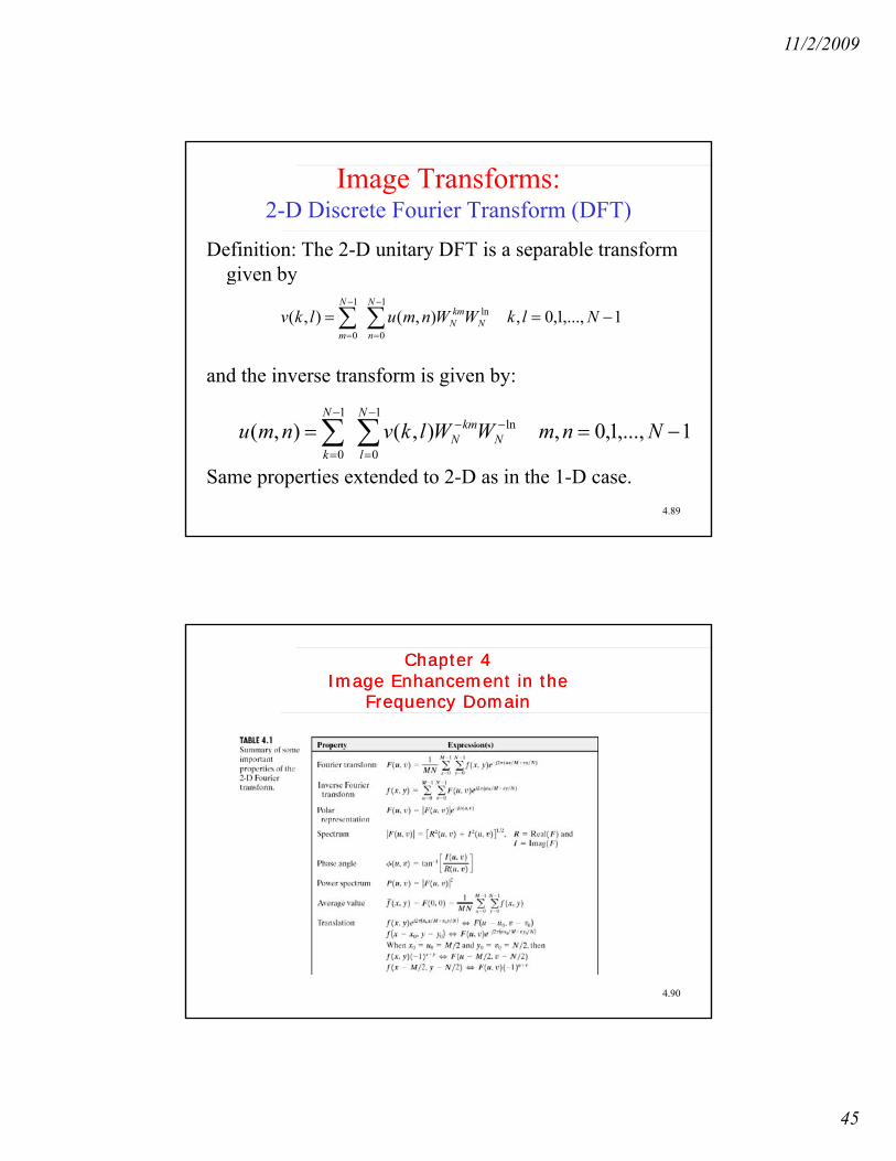
Image Transforms: 2-D Discrete Fourier Transform (DFT)
Definition: The 2-D unitary DFT is a separable transform given bygiven by
and the inverse transform is given by:
∑∑−
=
−
=
−==1
0
ln1
0
1,...,1,0,),(),(N
nN
kmN
N
m
NlkWWnmulkv
4.89
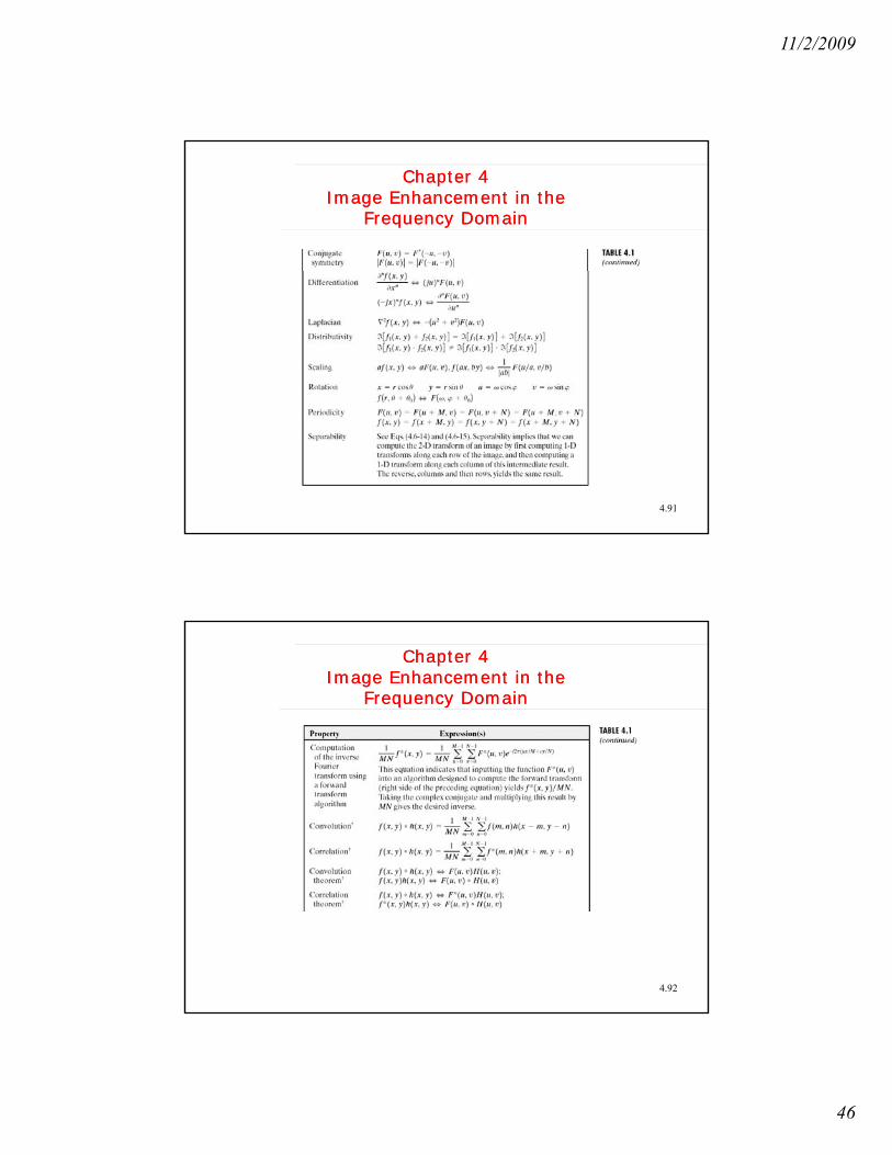
Same properties extended to 2-D as in the 1-D case.
∑∑−
=
−−−
=
−==1
0
ln1
01,...,1,0,),(),(
N
lN
kmN
N
kNnmWWlkvnmu
Chapter 4Image Enhancement in the
Frequency Domain
Chapter 4Image Enhancement in the
Frequency Domain
4.90
11/2/2009
46
Chapter 4Image Enhancement in the
Frequency Domain
Chapter 4Image Enhancement in the
Frequency Domain
4.91
Chapter 4Image Enhancement in the
Frequency Domain
Chapter 4Image Enhancement in the
Frequency Domain
4.92
11/2/2009
47
Chapter 4Image Enhancement in the
Frequency Domain
Chapter 4Image Enhancement in the
Frequency Domain
4.93
Chapter 4Image Enhancement in the
Frequency Domain
Chapter 4Image Enhancement in the
Frequency Domain
4.94
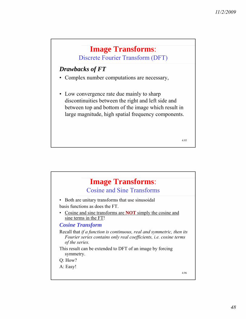
Note here that for n=15 (M=2n long sequence), FFT can be computed nearly 2200 times faster than direct DFT!
nnCn2)( =
The computational advantage of FFT over direct implementation of the 1-D DFT is defined as:
11/2/2009
48
Image Transforms: Discrete Fourier Transform (DFT)
Drawbacks of FT• Complex number computations are necessary,
• Low convergence rate due mainly to sharp discontinuities between the right and left side and between top and bottom of the image which result in
4.95
large magnitude, high spatial frequency components.
Image Transforms: Cosine and Sine Transforms
• Both are unitary transforms that use sinusoidalbasis functions as does the FT.basis functions as does the FT.• Cosine and sine transforms are NOT simply the cosine and
sine terms in the FT!Cosine TransformRecall that if a function is continuous, real and symmetric, then its
Fourier series contains only real coefficients, i.e. cosine terms of the series.
4.96
fThis result can be extended to DFT of an image by forcing
symmetry.Q: How?A: Easy!
11/2/2009
49
Image Transforms: Discrete Fourier Transform (DFT)
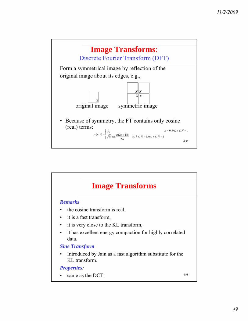
Form a symmetrical image by reflection of theoriginal image about its edges e goriginal image about its edges, e.g.,
original image symmetric imagex
x xx x
4.97
• Because of symmetry, the FT contains only cosine (real) terms:
⎪⎩
⎪⎨⎧
−≤≤−≤≤+
−≤≤==
10,112
)12(cos
10,0),(
2
1
NnNkN
knNnk
kncN
N
π
Image Transforms
Remarksth i t f i l• the cosine transform is real,
• it is a fast transform,• it is very close to the KL transform,• it has excellent energy compaction for highly correlated
data.Si T f
4.98
Sine Transform• Introduced by Jain as a fast algorithm substitute for the
KL transform.Properties:• same as the DCT.
11/2/2009
50
Image Transforms
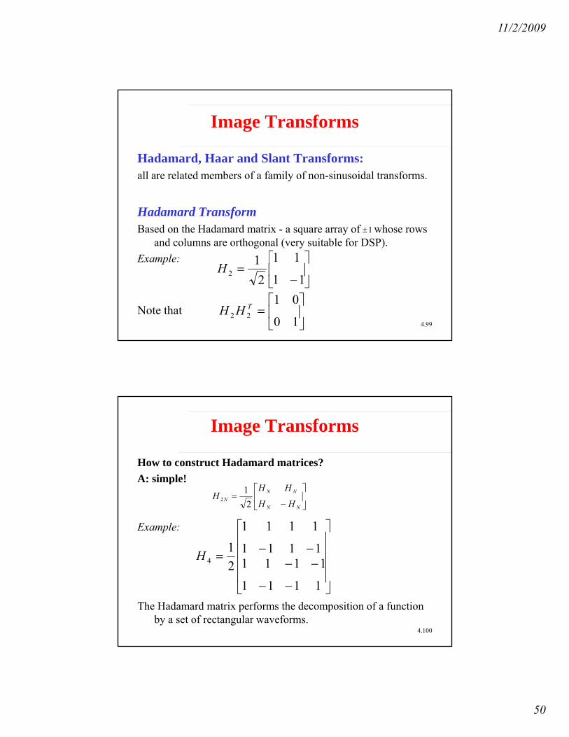
Hadamard, Haar and Slant Transforms:ll l t d b f f il f i id l t fall are related members of a family of non-sinusoidal transforms.
Hadamard TransformBased on the Hadamard matrix - a square array of whose rows
and columns are orthogonal (very suitable for DSP).E l ⎤⎡ 111
1±
4.99
Example:
Note that
⎥⎦
⎤⎢⎣
⎡
−=
11
11
21
2H
⎥⎦
⎤⎢⎣
⎡=
10
0122THH
Image Transforms
How to construct Hadamard matrices?A: simple!A: simple!
Example:
⎥⎦
⎤⎢⎣
⎡
−=
NN
NNN HH
HHH
21
2
⎥⎥⎥⎤
⎢⎢⎢⎡
−−= 111111
11
11
11
21
4H
4.100
The Hadamard matrix performs the decomposition of a function by a set of rectangular waveforms.
⎥⎥
⎦⎢⎢
⎣ −
−−
− 11
11
11
112

11/2/2009
51
Image Transforms
Note: some Hadamard matrices can be obtained by sampling the Walsh functions.Walsh functions.
Hadamard Transform Pairs:
where
∑−
=
−=−=1
0
),(1 1,...,1,0)1)(()(N
n
nkbN
Nknukv
∑−
=
−=−=1
0
),(1 1,...,1,0)1)(()(N
k
nkbN
Nnkvnu
10)(1
∑−m
kkkb
4.101
where
and {ki} {ni} are the binary representations of k and n, respectively, i.e.,
1,0,),(0
== ∑=
iii
ii nknknkb
11
1011
10 2222 −−
−− +++=+++= m
mm
m nnnnkkkk LL
Image TransformsProperties of Hadamard Transform:• it is real, symmetric and orthogonal,• it is a fast transform, and• it has good energy compaction for highly correlated images.
4.102

11/2/2009
52
Image TransformsHaar Transformis also derived from the (Haar) matrix:ex:
⎥⎥⎥⎥⎥
⎦
⎤
⎢⎢⎢⎢⎢
⎣
⎡
−
−−−
=
22
00
00
2211
11
11
11
21
4H
4.103
It acts like several “edge extractors” since it takes differences alongrows and columns of the local pixel averages in the image.
Image TransformsProperties of the Haar Transform:• it's real and orthogonal,• very fast, O(N) for N-point sequence!• it has very poor energy compaction.
4.104
11/2/2009
53
Image Transforms
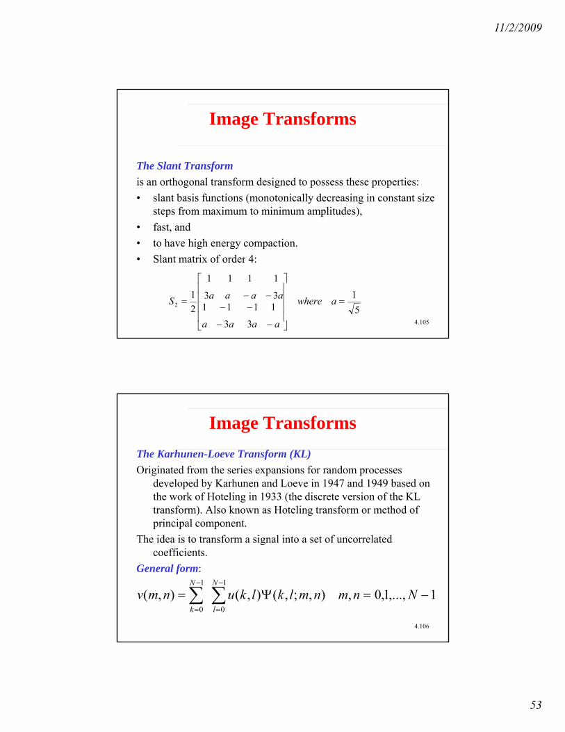
The Slant Transformis an orthogonal transform designed to possess these properties:• slant basis functions (monotonically decreasing in constant size
steps from maximum to minimum amplitudes),• fast, and• to have high energy compaction.
Sl i f d 4
4.105
• Slant matrix of order 4:
51
3
11
3
113
11
3
11
21
2 =
⎥⎥⎥⎥
⎦
⎤
⎢⎢⎢⎢
⎣
⎡
−
−
−
−−−= awhere
aaaa
aaaaS
Image TransformsThe Karhunen-Loeve Transform (KL)Originated from the series expansions for random processes
developed by Karhunen and Loeve in 1947 and 1949 based on the work of Hoteling in 1933 (the discrete version of the KL transform). Also known as Hoteling transform or method of principal component.
The idea is to transform a signal into a set of uncorrelated coefficients.
4.106
General form:
∑∑−
=
−
=
−=Ψ=1
0
1
01,...,1,0,),;,(),(),(
N
l
N
kNnmnmlklkunmv
11/2/2009
54
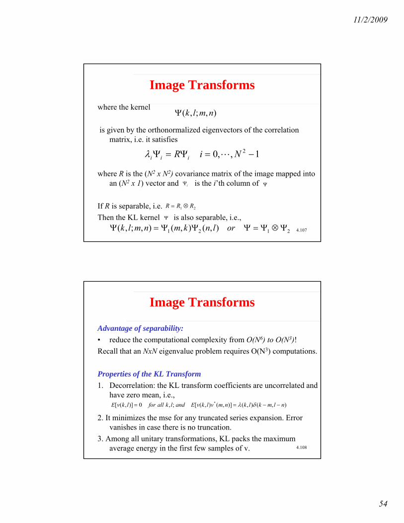
Image Transformswhere the kernel
),;,( nmlkΨ
is given by the orthonormalized eigenvectors of the correlation matrix, i.e. it satisfies
where R is the (N2 x N2) covariance matrix of the image mapped into an (N2 x 1) vector and is the i’th column of
1,,0 2 −=Ψ=Ψ NiR iii Lλ
Ψ
4.107
an (N2 x 1) vector and is the i th column of
If R is separable, i.e. Then the KL kernel is also separable, i.e.,
iΨ Ψ
Ψ
21 RRR ⊗=
2121 ),(),(),;,( Ψ⊗Ψ=ΨΨΨ=Ψ orlnkmnmlk
Image Transforms
Advantage of separability:• reduce the computational complexity from O(N6) to O(N3)!• reduce the computational complexity from O(N ) to O(N )!Recall that an NxN eigenvalue problem requires O(N3) computations.
Properties of the KL Transform1. Decorrelation: the KL transform coefficients are uncorrelated and
have zero mean, i.e.,
4.108
2. It minimizes the mse for any truncated series expansion. Error vanishes in case there is no truncation.
3. Among all unitary transformations, KL packs the maximum average energy in the first few samples of v.
),(),()],(),([;,0)],([ * nlmklknmvlkvEandlkallforlkvE −−== δλ

11/2/2009
55
Image Transforms
Drawbacks of KL:a) unlike other transforms the KL is image-dependent in fact ita) unlike other transforms, the KL is image-dependent, in fact, it
depends on the second order moments of the data,b) it is very computationally intensive.
4.109
Image Transforms
Singular Value Decomposition (SVD):SVD does for one image exactly what KL does for a set of imagesSVD does for one image exactly what KL does for a set of images.Consider an NxN image U. Let the image be real and M≤N.The matrix UUT and UTU are nonnegative, symmetric and have
identical eignevalues {λi}. There are at most r ≤M nonzero eigenvalues.
It is possible to find r orthogonal Mx1 eigenvectors {Фm} of UTU and
4.110
r orthogonal Nx1 eigenvectors {Ψm}of UUT, i.e.UTU Фm = λm Фm , m = 1, ..., r
and UUT Ψm= λm Ψm, m = 1, ..., r
11/2/2009
56
Image Transforms: SVD Cont’d
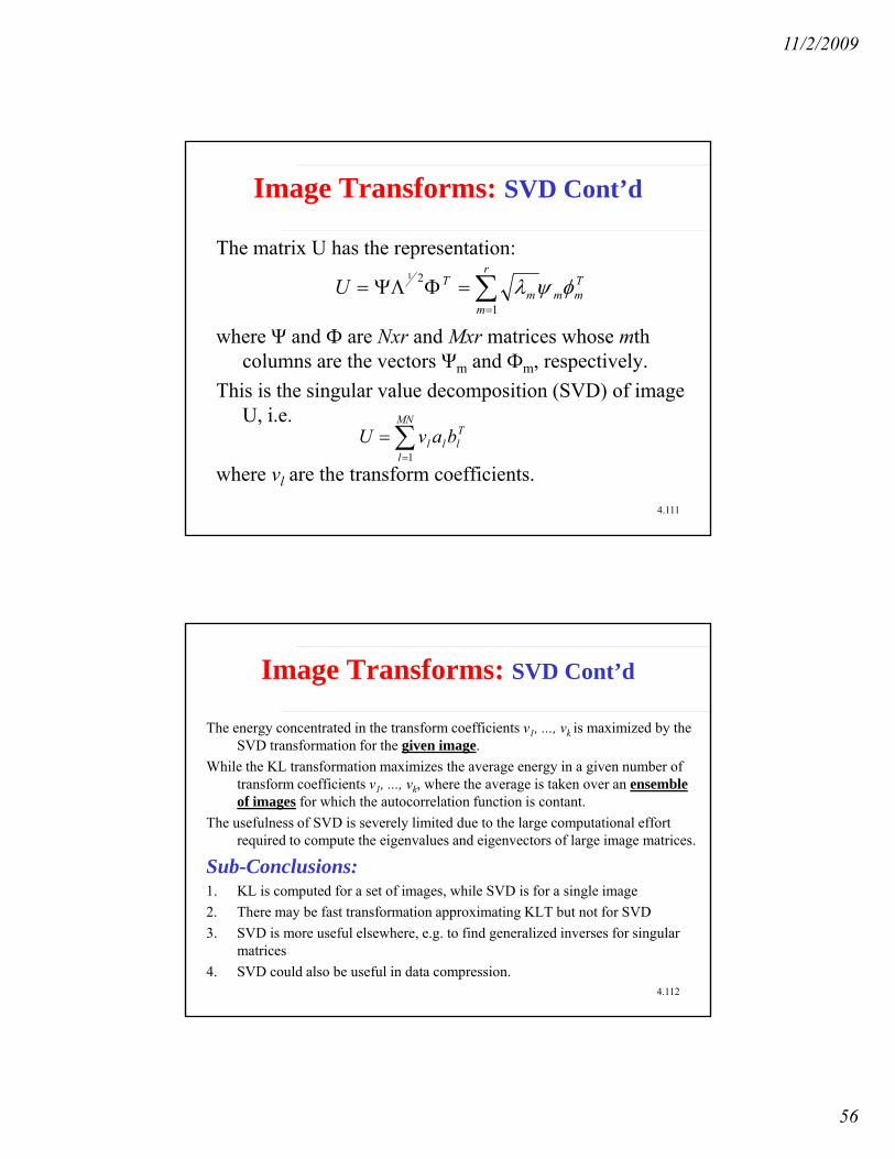
The matrix U has the representation:r
where Ψ and Ф are Nxr and Mxr matrices whose mth columns are the vectors Ψm and Фm, respectively.
This is the singular value decomposition (SVD) of image
∑=
=ΦΨΛ=r
m
Tmmm
TU1
21
φψλ
4.111
U, i.e.
where vl are the transform coefficients.
∑=
=MN
l
Tlll bavU
1
Image Transforms: SVD Cont’d
The energy concentrated in the transform coefficients v1, ..., vk is maximized by the SVD transformation for the given image.
While the KL transformation maximizes the average energy in a given number of transform coefficients v1, ..., vk, where the average is taken over an ensemble of images for which the autocorrelation function is contant.
The usefulness of SVD is severely limited due to the large computational effortrequired to compute the eigenvalues and eigenvectors of large image matrices.
Sub-Conclusions:1 KL i d f f i hil SVD i f i l i
4.112
1. KL is computed for a set of images, while SVD is for a single image2. There may be fast transformation approximating KLT but not for SVD3. SVD is more useful elsewhere, e.g. to find generalized inverses for singular
matrices4. SVD could also be useful in data compression.

11/2/2009
57
Image Transforms
Evaluation and Comparison of Different TransformsPerformance of different unitary transforms with repect to basisPerformance of different unitary transforms with repect to basis
restriction errors (Jm) versus the number of basis (m) for a stationary Markov sequence with N=16 and correlation coefficient 0.95.
1,,0,12
12
−==
∑
∑−
−
= NmJ N
k
N
mkk
m L
σ
σ
4.113
where the variaces have been arranged in decreasing order.0∑=k
k
Image Transforms
Evaluation and Comparison of Different TransformsSee Figs 5 19-5 23See Figs. 5.19-5.23.
4.114

11/2/2009
58
Image TransformsEvaluation and Comparison of Different Transforms
Zonal FilteringZonal Mask:Zonal Mask:
energytotalstopbandinenergy
v
vJ N
lk
stopbandlklk
s ==
∑∑
∑∑−
∈1 2
,
,
2,
Define the normalized MSE:
4.115
lk∑∑=0,
Zonal Filtering with DCT transform
(a) Original image;
(b) 4:1 sample reduction;
4.116
(c) 8:1 sample reduction;
(d) 16:1 sample reduction.
Figure Basis restriction zonal filtered images in cosine transform domain.
11/2/2009
59
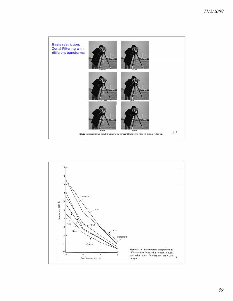
Basis restriction:Zonal Filtering with different transforms
(a) Cosine; (b) sine;
(c) unitary DFT; (d) Hadamard;
4.117(e) Haar; (f) Slant.
Figure Basis restriction zonal filtering using different transforms with 4:1 sample reduction.
Image Transforms
4.118

11/2/2009
60
TABLE - Summary of Image Transforms
DFT/unitary DFT Fast transform, most useful in digital signal processing, convolution, digital filtering, analysis of circulant and Toeplitz systems. Requires complex arithmetic. Has very good energy compaction for images.
Cosine Fast transform, requires real operations, near optimal substitute for the KL transform of highly correlated images. Useful in designing transform coders and Wiener filters for images. Has excellent energy compaction for images.
Sine About twice as fast as the fast cosine
4.119
transform, symmetric, requires real operations; yields fast KL transform algorithm which yields recursive block processing algorithms, for coding, filtering, and so on; useful in estimating performance bounds of many image processing problems. Energy compaction for images is very good.
Hadamard Faster than sinusoidal transforms, since no multiplications are required; useful in digital hardware implementations of image processing algorithms. Easy to simulate but difficult to analyze. Applications in image data compression, filtering, and design of codes. Has good energy compaction for imagescompaction for images.
Haar Very fast transform. Useful in feature extraction, image coding, and image analysis problems. Energy compaction is fair.
4.120
Slant Fast transform. Has “image-like basis”; useful in image coding. Has very good energy compactionfor images

11/2/2009
61
Karhunen-Loeve Is optimal in many ways; has no fast algorithm; useful in performance evaluation and for finding performance bounds. Useful for small size vectors e.g., color multispectral or other feature vectors. Has the best energy compaction in the mean square sense over an ensemble.
Fast KL Useful for designing fast, recursive-block processing techniques, g g , p g q ,including adaptive techniques. Its performance is better than independent block-by-block processing techniques.
SVD transform Best energy-packing efficiency for any given image. Varies drastically from image to image; has no fast algorithm or a reasonable fast transform substitute; useful in design of separable FIR filters, finding least squares and minimum norm solutions of linear equations, finding rank of large matrices, and so on. Potential image processing applications are in image restoration, power spectrum estimation and data compression
4.121
power spectrum estimation and data compression.
Image Transforms
Conclusions1. It should often be possible to find a sinusoidal transform
as a good substitute for the KL transform2. Cosine Transform always performs best!3. All transforms can only be appreciated if individually
experimented with
4.122
4. Singular Value Decomposition (SVD) is a transformwhich locally (per image) achieves pretty much whatthe KL does for an ensemble of images (i.e., decorrelation).