Embed Size (px)
Citation preview

Fourier Analysis & Discrete-time Systems
Road map – looking backwards Continuous-time signals & systems
Ordinary differential equations Integrating factors, variation of parameters
State-space and vector ODEs
Zero-input response + zero-state response
Impulse response, step response
Convolution
Laplace transform methods
Transfer functions, poles, zeros
Partial fraction expansion
Frequency response, sinusoidal steady-state, Bode diagrams Filtering; lowpass, highpass, etc
Signals & systems; inputs, states, outputs, responses MAE143A Signals & Systems Winter 2015 1

Fourier Analysis & Discrete-time Systems
Road map – looking forwards Sampling and discrete-time signals
Periodic signals & Fourier series Complex Fourier series
Line spectrum, Parseval
Frequency response
Fourier transform
bandlimited, convolution
Periodically sampled signals
Fourier transform of sampled signals
ADC, lowpass filtering
sampling and reconstruction
Aliasing
Discrete Fourier Transform (DFT/FFT)
MAE143A Signals & Systems Winter 2015 2
Chaparro 4.3 4.4 4.9 5.2 5.7 7.2 7.4 7.2-7.3 10.2-10.4
Fourier Analysis & Discrete-time Systems
Road map – looking forwards Discrete-time signals & systems
Ordinary difference equations Direct solution
State-space and vector ODEs
Zero-input response + zero-state response
Impulse response, step response
Convolution
Z-transform methods
Transfer functions, poles, zeros
Partial fraction expansion
Frequency response, sinusoidal steady-state, Bode diagrams Filtering; lowpass, highpass, etc
Signals & systems; inputs, states, outputs, responses MAE143A Signals & Systems Winter 2015 3

Moving from continuous- to discrete-time
Sampling ideas Uniform, periodic sampling rate, e.g. CDs at 44.1KHz
First we will need to consider periodic signals in order to appreciate how to interpret discrete-time signals as representative of continuous-time
Fourier series and transforms
Discrete-time Fourier transform (DTFT)
Discrete Fourier transform (DFT) & the fast Fourier transform (FFT)
Aliasing and signal reconstruction
Discrete-time signals then discrete-time systems Matlab tools and digital signal processing
Nothing on digital (finite bit-length) signals
MAE143A Signals & Systems Winter 2015 4
Fourier series for periodic signals (Chap 3)
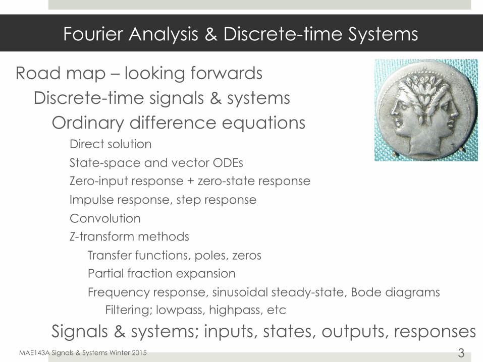
Periodic signal For all times Period here is 6 sec
Smallest possible repetition time
The signal is real
Fourier series representation Sometimes called the complex Fourier series representation
MAE143A Signals & Systems Winter 2015 5
x(t+ T ) = x(t), 8t 2 (�1,1)
t 2 (�1,1)
x(t) =1X
k=�1cke
jk�0t, t 2 (�1,1), ⇥0 =2�
T

Fourier series for periodic signals
Signal x(t) is periodic with fundamental period T
Fourier coefficients are complex numbers Since x(t) is real
The trigonometric Fourier series
MAE143A Signals & Systems Winter 2015 6
x(t) =1X
k=�1cke
jk�0t, t 2 (�1,1), ⇥0 =2�
T
ck =1
T
Z T
0x(t)e�jk!0t
dt, k = . . . ,�2,�1, 0, 1, 2, . . .
c�k = c̄k
x(t) = c0 + 2
1X
k=1
|ck| cos(k!0t+ \ck), t 2 (�1,1)
= a0 +
1X
k=1
[ak cos(k!0t) + bk sin(k!0t)]
The complex exponential Fourier series
MAE143A Signals & Systems Winter 2015 7
x(t) =1X
k=�1cke
jk�0t, t 2 (�1,1), ⇥0 =2�
T
ck =1
T
Z T
0x(t)e�jk!0t
dt, k = . . . ,�2,�1, 0, 1, 2, . . .
The Phantom is not afraid of complex numbers
He always uses the complex Fourier series representation of periodic signals
So do we!
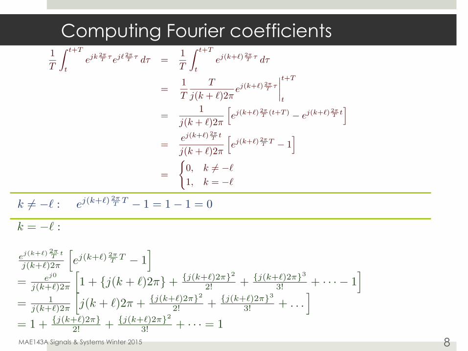
Computing Fourier coefficients
MAE143A Signals & Systems Winter 2015 8
1T
Z t+T
tejk 2⇡
T ⌧ej` 2⇡T ⌧ d⌧ =
1T
Z t+T
tej(k+`) 2⇡
T ⌧ d⌧
=1T
T
j(k + `)2⇡ej(k+`) 2⇡
T ⌧
����t+T
t
=1
j(k + `)2⇡
hej(k+`) 2⇡
T (t+T ) � ej(k+`) 2⇡T t
i
=ej(k+`) 2⇡
T t
j(k + `)2⇡
hej(k+`) 2⇡
T T � 1i
=
(0, k 6= �`
1, k = �`
k 6= �` : ej(k+`) 2⇡T T � 1 = 1� 1 = 0
k = �` :
ej(k+`) 2⇡T
t
j(k+`)2⇡
hej(k+`) 2⇡
T T � 1i
= ej0
j(k+`)2⇡
h1 + {j(k + `)2⇡} + {j(k+`)2⇡}2
2! + {j(k+`)2⇡}3
3! + · · ·� 1i
= 1j(k+`)2⇡
hj(k + `)2⇡ + {j(k+`)2⇡}2
2! + {j(k+`)2⇡}3
3! + . . .i
= 1 + {j(k+`)2⇡}2! + {j(k+`)2⇡}2
3! + · · · = 1

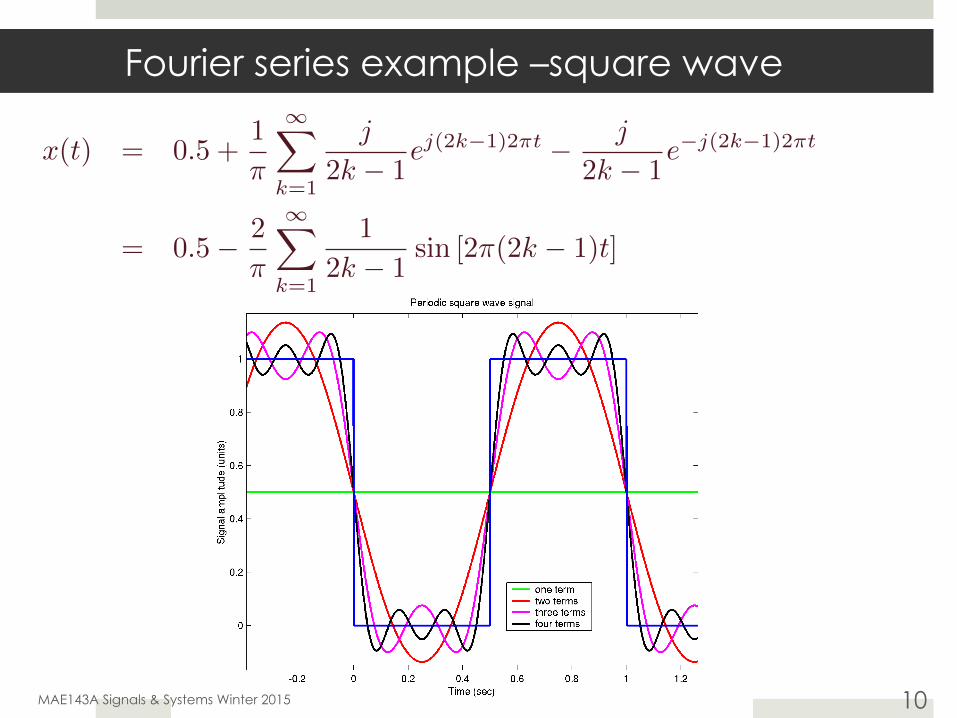
Fourier series example – square wave
T=1, ω0=2π
Compute coefficients
MAE143A Signals & Systems Winter 2015 9
x(t) =
(0, t 2 (0, 0.5]
1, t 2 (0.5, 1]
c0 =1
1
Z 1
0x(t) dt =
Z 1
0.5dt = 0.5
ck =
Z 1
0x(t)e
�jk2⇡tdt =
Z 1
0.5e
�jk2⇡tdt =
1
�jk2⇡
e
�jk2⇡t
����1
0.5
=
1
�jk2⇡
�e
�jk2⇡ � e
�jk⇡�=
(jk⇡ , k odd
0, k even
k = . . . ,�2,�1, 1, 2, . . .
Fourier series example –square wave
MAE143A Signals & Systems Winter 2015 10
x(t) = 0.5 +1
�
1X
k=1
j
2k � 1ej(2k�1)2�t � j
2k � 1e�j(2k�1)2�t
= 0.5� 2
�
1X
k=1
1
2k � 1sin [2�(2k � 1)t]
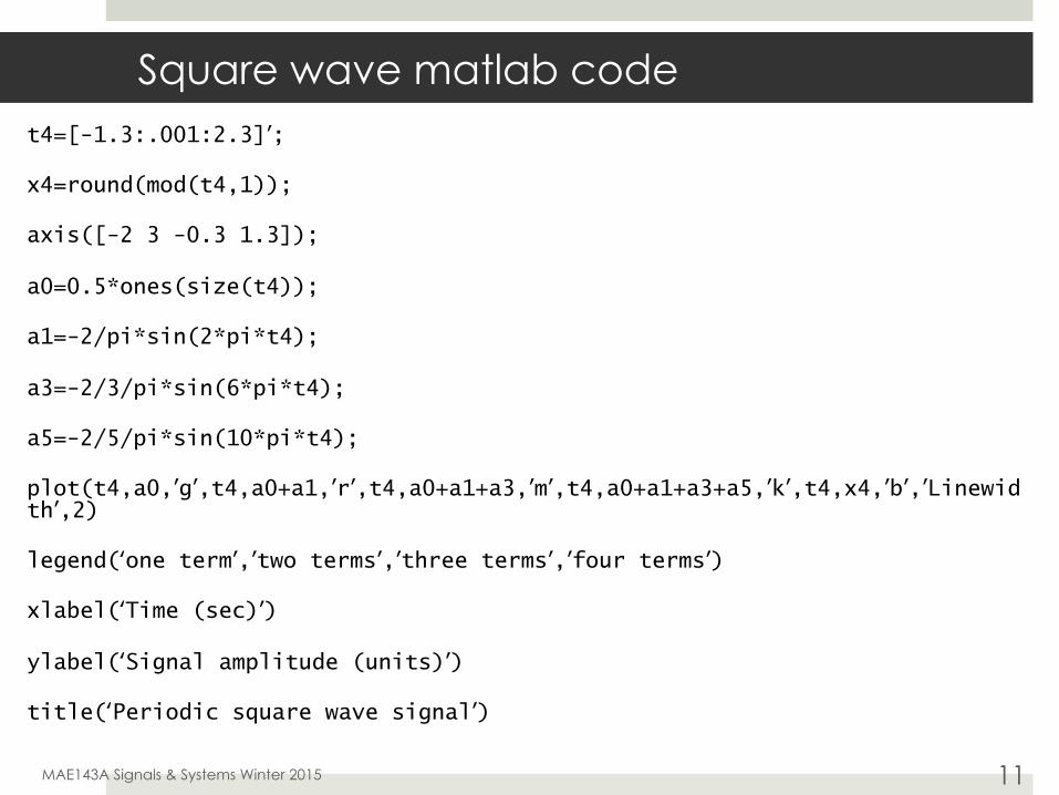
Square wave matlab code t4=[-1.3:.001:2.3]ʼ’;
x4=round(mod(t4,1));
axis([-2 3 -0.3 1.3]);
a0=0.5*ones(size(t4));
a1=-2/pi*sin(2*pi*t4);
a3=-2/3/pi*sin(6*pi*t4);
a5=-2/5/pi*sin(10*pi*t4);
plot(t4,a0,ʼ’gʼ’,t4,a0+a1,ʼ’rʼ’,t4,a0+a1+a3,ʼ’mʼ’,t4,a0+a1+a3+a5,ʼ’kʼ’,t4,x4,ʼ’bʼ’,ʼ’Linewidthʼ’,2)
legend(ʻ‘one termʼ’,ʼ’two termsʼ’,ʼ’three termsʼ’,ʼ’four termsʼ’)
xlabel(ʻ‘Time (sec)ʼ’)
ylabel(ʻ‘Signal amplitude (units)ʼ’)
title(ʻ‘Periodic square wave signalʼ’)
MAE143A Signals & Systems Winter 2015 11
MAE143A Signals & Systems Winter 2015 12 MAE143A Signals & Systems Winter 2005
12
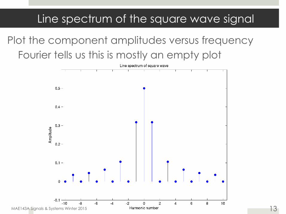
Line spectrum of the square wave signal
Plot the component amplitudes versus frequency Fourier tells us this is mostly an empty plot
MAE143A Signals & Systems Winter 2015 13
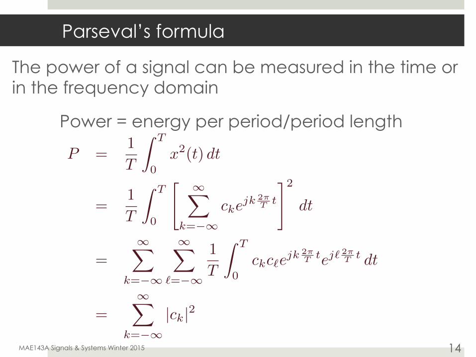
Parseval’s formula
The power of a signal can be measured in the time or in the frequency domain
Power = energy per period/period length
MAE143A Signals & Systems Winter 2015 14
P =1
T
Z T
0x
2(t) dt
=1
T
Z T
0
" 1X
k=�1cke
jk 2⇡T t
#2
dt
=1X
k=�1
1X
`=�1
1
T
Z T
0ckc`e
jk 2⇡T t
e
j` 2⇡T t
dt
=1X
k=�1|ck|2
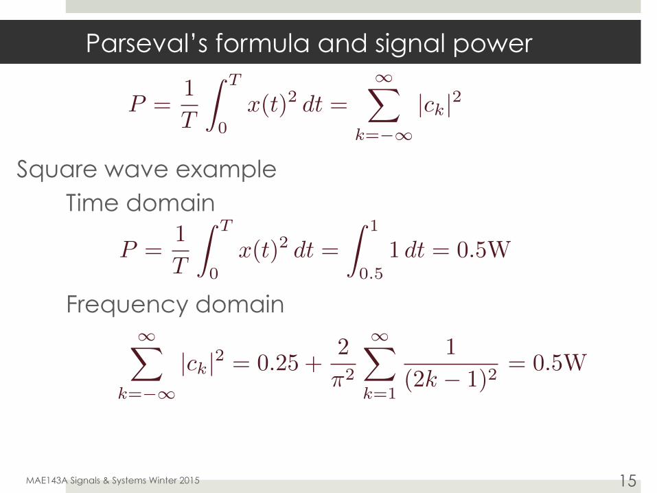
Parseval’s formula and signal power
Square wave example Time domain Frequency domain
MAE143A Signals & Systems Winter 2015 15
P =1
T
Z T
0x(t)2 dt =
1X
k=�1|ck|2
P =1
T
Z T
0x(t)2 dt =
Z 1
0.51 dt = 0.5W
1X
k=�1|ck|2 = 0.25 +
2
�2
1X
k=1
1
(2k � 1)2= 0.5W
Summary of Fourier series
Write a periodic signal as an infinite sum of complex exponentials at harmonic frequencies
The line spectrum depicts the frequency content Parseval tells us this captures all the energy properly
A linear system with periodic input (not just sinusoidal) will have a steady-state response which is the sum of the individual s-s-s responses
The contribution from each component is given by the systems frequency response
MAE143A Signals & Systems Winter 2015 16

Frequency response example
MAE143A Signals & Systems Winter 2015 17
System 1: G1(s) =20
s+ 20
System 2: G2(s) =23000
s+ 20s+ 23000
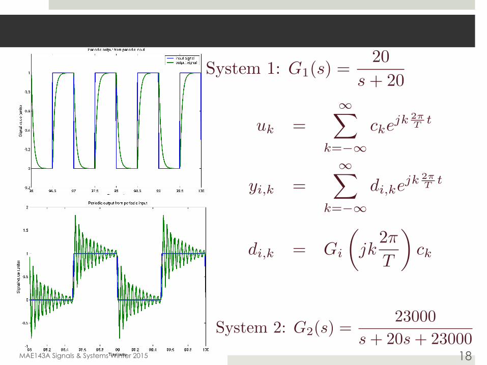
MAE143A Signals & Systems Winter 2015 18
System 1: G1(s) =20
s+ 20
System 2: G2(s) =23000
s+ 20s+ 23000
uk =1X
k=�1cke
jk 2⇡T t
yi,k =1X
k=�1di,ke
jk 2⇡T t
di,k = Gi
✓jk
2⇡
T
◆ck
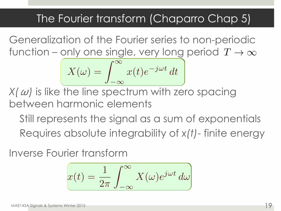
The Fourier transform (Chaparro Chap 5)
Generalization of the Fourier series to non-periodic function – only one single, very long period
X(ω) is like the line spectrum with zero spacing between harmonic elements
Still represents the signal as a sum of exponentials Requires absolute integrability of x(t)- finite energy
Inverse Fourier transform
MAE143A Signals & Systems Winter 2015 19
T ! 1
X(�) =
Z 1
�1x(t)e�j�t dt
x(t) =1
2⇡
Z 1
�1X(!)ej!t
d!

The Fourier transform - example
Two-sided decaying exponential
MAE143A Signals & Systems Winter 2015 20
X(!) =
Z 1
�1e�
|t|5 e�j!t dt
=
Z 0
�1e
t5�j!t dt+
Z 1
0e�
t5�j!t dt
=�1
j! � 15
+1
j! + 15
|X(!)| =25
!2 + 125
x(t) = e
� |t|5, t 2 (�1,1)

The Fourier and Laplace transforms
For a one-sided signal x(t)with Laplace transform
Note that this is a signal property It mimics the Laplace transform and frequency response relationship for causal systems
The interest in Fourier transforms is in the infinite-time response to periodic inputs
Special Fourier transforms
MAE143A Signals & Systems Winter 2015 21
X(!) = X (s)|s=j!
X (s)
Y (!) = H(j!)U(!), H(!) = F(h(t))
F [�(t)] = 1, F [cos!0t] = ⇡[�(! � !0) + �(! + !0)]
F [1] = 2⇡�(!), F [sin!0t] = j⇡[��(! � !0) + �(! + !0)]

Bandlimited signals
Signals, x(t), whose Fourier transform, X(ω), is zero for frequencies outside a value, the bandwidth, B, i.e.
is referred to as bandlimited
A periodic signal with line spectrum zero outside the bandwidth B is also referred to as bandlimited
Bandlimited implies a level of smoothness (as we shall see in the homework)
Fourier series: finite power, periodic
Fourier transform: finite energy, one-shot MAE143A Signals & Systems Winter 2015 22
X(!) = 0 for {! > B} [ {! < �B}

Convolution and the Fourier transform
The same as for the Laplace transform
MAE143A Signals & Systems Winter 2015 23
x(t) ⇤ y(t) =Z 1
�1x(t� ⌧)y(⌧) d⌧ = F�1 [X(!)Y (!)]
F(x ⇥ y) =
Z 1
�1
Z 1
�1x(t� ⇥)y(⇥) d⇥
�e�j⇤t dt
=
Z 1
�1
Z 1
�1x(t� ⇥)e�j⇤(t�⇥)y(⇥)e�j⇤⇥ d⇥ dt
=
Z 1
�1x(t� ⇥)e�j⇤(t�⇥) dt
Z 1
�1y(⇥)e�j⇤⇥ d⇥
=
Z 1
�1x(�)e�j⇤� d�
Z 1
�1y(⇥)e�j⇤⇥ d⇥
= X(⇤)Y (⇤)
� = t� ⌧d� = �d⌧,⌧ = �1 ! � = 1⌧ = 1 ! � = �1

Convolution and the Fourier transform II
Using the symmetry between and
MAE143A Signals & Systems Winter 2015 24
X(�) =
Z 1
�1x(t)e�j�t dt x(t) =
1
2⇡
Z 1
�1X(!)ej!t
d!
F F�1
F [x(t)y(t)] =1
2⇡X(!) ⇤ Y (!) =
1
2⇡
Z 1
�1X(! � �)Y (�) d�
F [x(t)y(t)] =
Z 1
t,�1x(t)y(t)e�j!t
dt
=
Z 1
t,�1
1
2⇡
Z 1
⇢,�1X(⇢)ej⇢t d⇢
� 1
2⇡
Z 1
�,�1Y (�)ej�t d�
�e
�j!tdt
=1
4⇡2
Z 1
⇢,�1X(⇢)
⇢Z 1
�,�1Y (�)
Z 1
t,�1e
�j!te
j⇢te
j�tdt
�d�
�d⇢
=1
4⇡2
Z 1
⇢,�1X(⇢)
⇢Z 1
�,�1Y (�)⇥ 2⇡�(⇢+ � � !) d�
�d⇢
=1
2⇡
Z 1
⇢,�1X(⇢)Y (! � ⇢) d⇢ =
1
2⇡X(!) ⇤ Y (!)
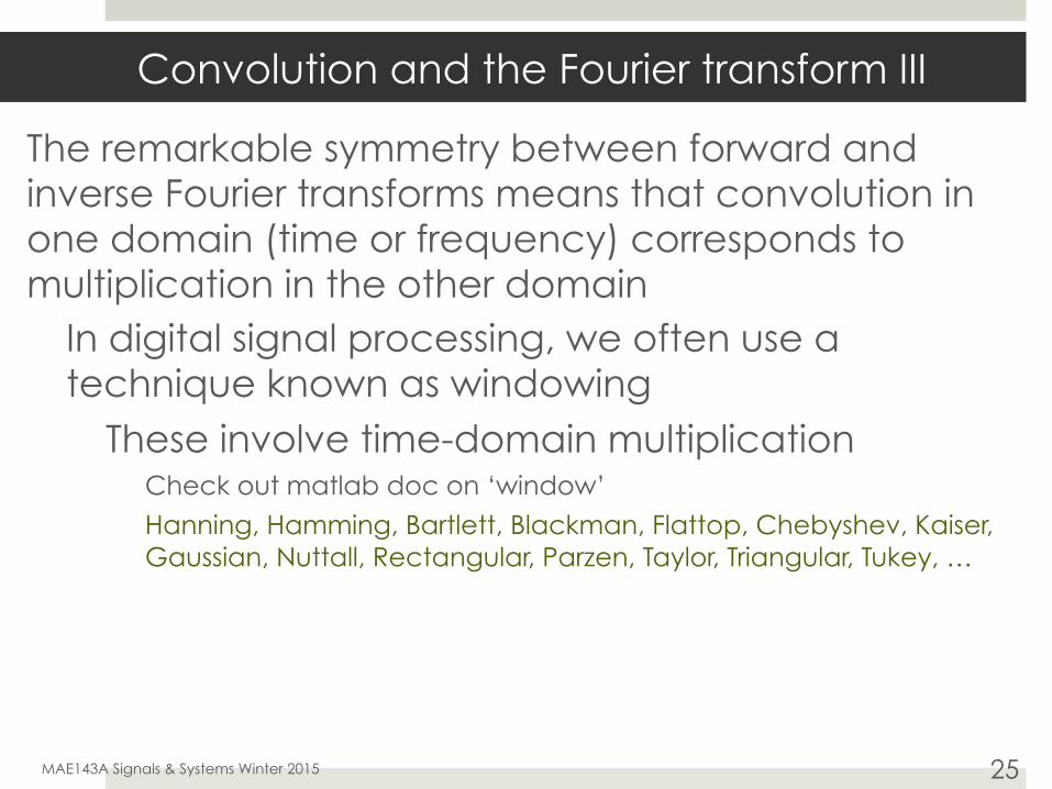
Convolution and the Fourier transform III
The remarkable symmetry between forward and inverse Fourier transforms means that convolution in one domain (time or frequency) corresponds to multiplication in the other domain
In digital signal processing, we often use a technique known as windowing
These involve time-domain multiplication Check out matlab doc on ‘window’
Hanning, Hamming, Bartlett, Blackman, Flattop, Chebyshev, Kaiser, Gaussian, Nuttall, Rectangular, Parzen, Taylor, Triangular, Tukey, …
MAE143A Signals & Systems Winter 2015 25

Sampled signals – discrete time
For computer use we need to sample signals Most commonly this is periodic sampling every T seconds we take a sample of the continuous signal This yields a sequence
A continuous-time signal is a function of time t A discrete-time signal is a sequence indexed by t
T is the sampling period (sec)
1/T is the sample rate (Hz)
Often we also quantize the samples to yield a digital signal of a fixed number of bits representation
This is a subject for the next course
MAE143A Signals & Systems Winter 2015 26
xn = x(nT )
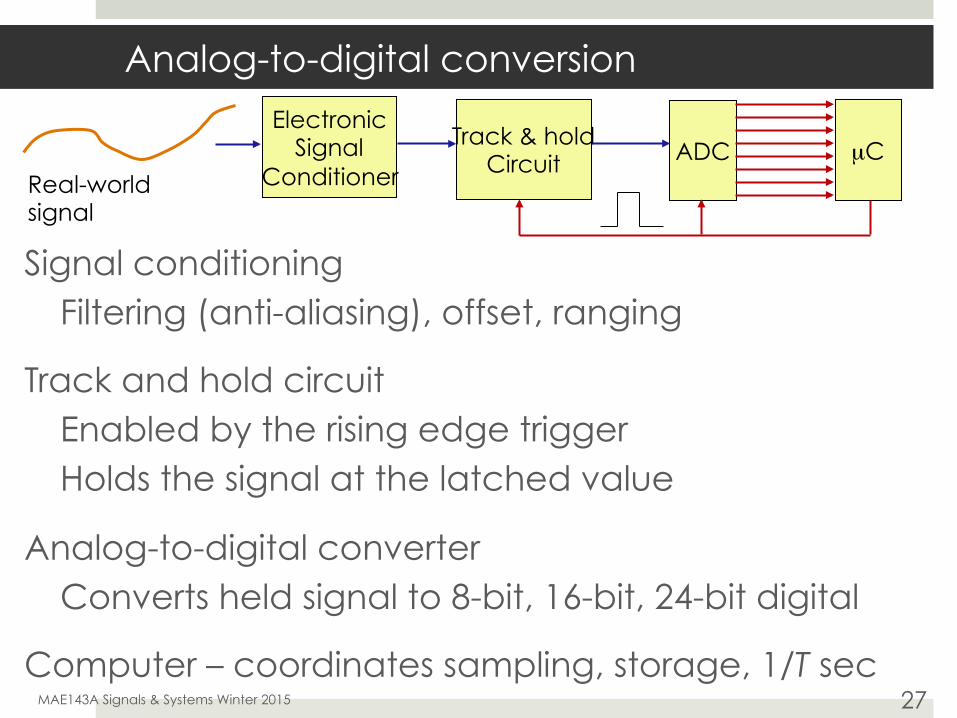
Analog-to-digital conversion
Signal conditioning Filtering (anti-aliasing), offset, ranging
Track and hold circuit Enabled by the rising edge trigger Holds the signal at the latched value
Analog-to-digital converter Converts held signal to 8-bit, 16-bit, 24-bit digital
Computer – coordinates sampling, storage, 1/T sec MAE143A Signals & Systems Winter 2015 27
Electronic Signal
Conditioner Real-world signal
Track & hold Circuit ADC µC

Ideal sampling of signals
Continuous-time signal x(t) Continuous values of x, t
Discrete-time signal xn
Continuous x, integer n A sequence
Sampled-data signal xs(t) Continuous x, t Modeled by a pulse train
MAE143A Signals & Systems Winter 2015 28
t
x(t)
t
xs(t)
0 T 2T 3T 4T 5T 6T 7T -T -2T
xn
0 1 2 3 4 5 6 7 -1 -2 n
xs(t) =1X
n=�1xn�(t� nT ) = x(t)⇥
1X
n=�1�(t� nT )

Fourier transform of a sampled signal
Fourier transform of a product is the convolution of the Fourier transforms
What is the Fourier series of periodic pulse train p(t)?
MAE143A Signals & Systems Winter 2015 29
xs(t) =1X
n=�1xn�(t� nT ) = x(t)⇥
1X
n=�1�(t� nT ) = x(t)p(t)
p(t) =1X
k=�1cke
jkwst
ck =1T
Z T/2
�T/2p(t)e�jk!st dt =
1T
p(t) =1X
k=�1
1T
ejk!st
Fourier transform of a sampled signal
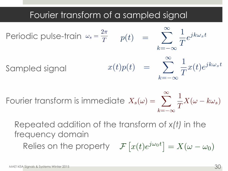
Periodic pulse-train
Sampled signal
Fourier transform is immediate Repeated addition of the transform of x(t) in the frequency domain
Relies on the property
MAE143A Signals & Systems Winter 2015 30
!s =2⇡
T
F⇥x(t)ej!0t
⇤= X(! � !0)
p(t) =1X
k=�1
1T
ejk!st
x(t)p(t) =1X
k=�1
1T
x(t)ejk!st
Xs(!) =1X
k=�1
1T
X(! � k!s)
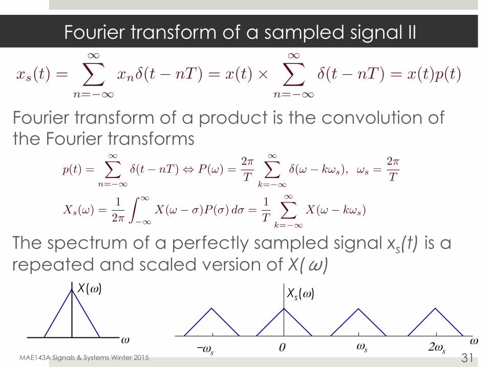
Fourier transform of a sampled signal II
Fourier transform of a product is the convolution of the Fourier transforms
The spectrum of a perfectly sampled signal xs(t) is a repeated and scaled version of X(ω)
MAE143A Signals & Systems Winter 2015 31
xs(t) =1X
n=�1xn�(t� nT ) = x(t)⇥
1X
n=�1�(t� nT ) = x(t)p(t)
X(ω)
ω
Xs(ω)
ωωs 2ωs-ωs 0
p(t) =1X
n=�1�(t� nT ) , P (!) =
2⇡
T
1X
k=�1�(! � k!s), !s =
2⇡
T
Xs(!) =1
2⇡
Z 1
�1X(! � �)P (�) d� =
1
T
1X
k=�1X(! � k!s)
Fourier transform of a sampled signal III
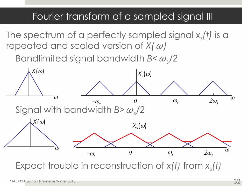
The spectrum of a perfectly sampled signal xs(t) is a repeated and scaled version of X(ω)
Bandlimited signal bandwidth B<ωs/2 Signal with bandwidth B>ωs/2
Expect trouble in reconstruction of x(t) from xs(t)
MAE143A Signals & Systems Winter 2015 32
X(ω)
ω
Xs(ω)
ωωs 2ωs-ωs 0
X(ω)
ω
Xs(ω)
ωωs 2ωs-ωs 0
Reconstructing sampled bandlimited signals
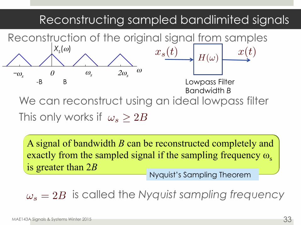
Reconstruction of the original signal from samples
We can reconstruct using an ideal lowpass filter This only works if
is called the Nyquist sampling frequency
MAE143A Signals & Systems Winter 2015 33
Xs(ω)
ωωs 2ωs-ωs 0B -B
H(!)x(t)xs(t)
Lowpass Filter Bandwidth B
!s � 2B
A signal of bandwidth B can be reconstructed completely and exactly from the sampled signal if the sampling frequency ωs is greater than 2B
Nyquist’s Sampling Theorem
!s = 2B

Ideal lowpass filter I
Ideal lowpass filter
MAE143A Signals & Systems Winter 2015 34
H(!)x(t)xs(t)
Lowpass Filter Bandwidth B
-B B
h(t) =1
2⇡
Z 1
�1H(!)e�j!t d! =
A
2⇡
Z B
�Be�j!t d!
=A
2⇡
1
�jte�j!t
����B
�B
=A
2⇡
2
t
1
2j
⇥ejBt � e�jBt
⇤
=AB
⇡
sinBt
Bt
4=
AB
⇡sincBt
H(!)
!
A
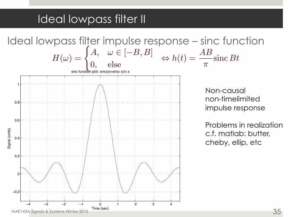
Ideal lowpass filter II
Ideal lowpass filter impulse response – sinc function
MAE143A Signals & Systems Winter 2015 35 −4 −3 −2 −1 0 1 2 3 4
−0.2
0
0.2
0.4
0.6
0.8
1
Time (sec)
Sign
al (u
nits
)
sinc function plot: sinc(x)=sin(! x)/! x
H(!) =
(A, ! 2 [�B,B]
0, else, h(t) =
AB
⇡sincBt
Non-causal non-timelimited impulse response Problems in realization c.f. matlab: butter, cheby, ellip, etc

Shannon’s interpolation formula
Convolution formula
MAE143A Signals & Systems Winter 2015 36
H(!)x(t)xs(t)
Lowpass Filter Bandwidth B
x(t) = h(t) ⇤ xs(t)
=
Z 1
�1
⇢BT
⇡
sinc
B
⇡
(t� ⌧)
��( 1X
n=�1x(nT )�(⌧ � nT )
)d⌧
=BT
⇡
1X
n=�1x(nT )
⇢Z 1
�1sinc
B
⇡
(t� ⌧)
��(⌧ � nT ) d⌧
�
=BT
⇡
1X
n=�1x(nT ) sinc
B
⇡
(t� nT )
�
Sampling and reconstruction
If the continuous-time signal is bandlimited to B and we sample faster than the Nyquist frequency
Then we can exactly reconstruct the original signal from the sample sequence
Conversely: if we sample at or more slowly than the Nyquist frequency then we cannot reconstruct the original signal from the samples alone
We might have other information that helps the reconstruction. Without such extra information we suffer from Aliasing – some frequencies masquerading as others
MAE143A Signals & Systems Winter 2015 37
Aliasing
Sampling rate is less than the Nyquist rate Spectra overlap in sampled signal Impossible to disentangle
Signals from above ωs/2 masquerade as signals of a lower frequency
This is what happens to wagon wheels in western movies
fs=30Hz but the passing rate of the spokes is greater than this
Dopplegänger and impersonation
Alias: a false or assumed identity
Samuel Langhorne Clemens alias Mark Twain
5.5KHz sampled at 10KHz a.k.a. 4.5KHz
MAE143A Signals & Systems Winter 2015 38
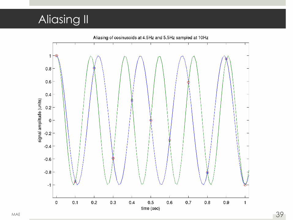
Aliasing II
MAE143A Signals & Systems Winter 2015 39
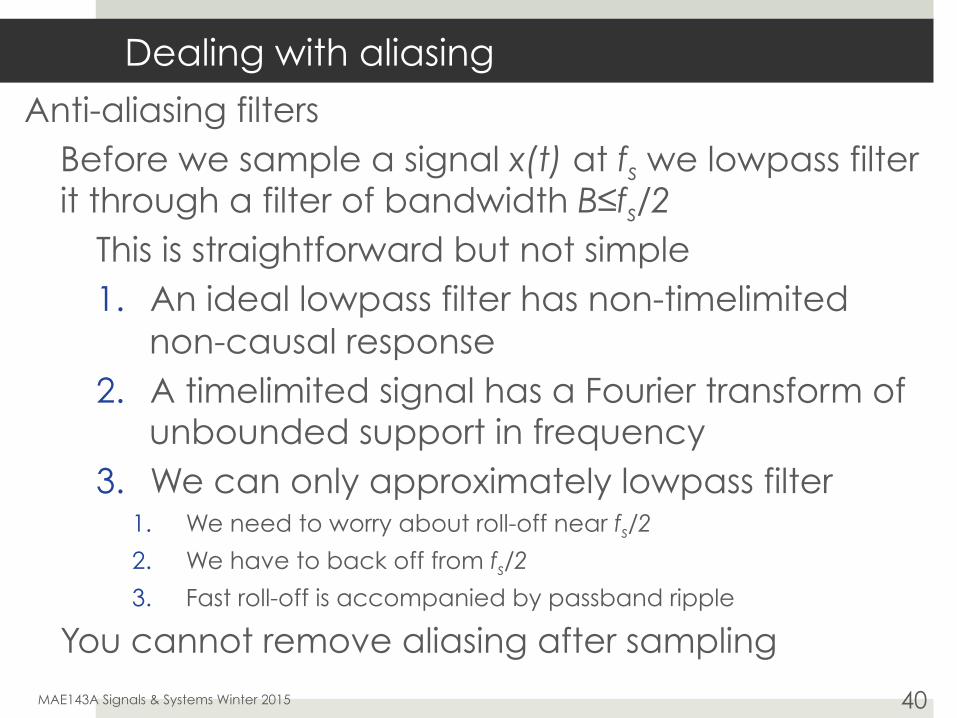
Dealing with aliasing
Anti-aliasing filters Before we sample a signal x(t) at fs we lowpass filter it through a filter of bandwidth B≤fs/2
This is straightforward but not simple 1. An ideal lowpass filter has non-timelimited
non-causal response 2. A timelimited signal has a Fourier transform of
unbounded support in frequency 3. We can only approximately lowpass filter
1. We need to worry about roll-off near fs/2
2. We have to back off from fs/2
3. Fast roll-off is accompanied by passband ripple
You cannot remove aliasing after sampling
MAE143A Signals & Systems Winter 2015 40

Aliasing in practice
Any data-logging equipment worth a dime has anti-aliasing filtering built in
It is switched in at sample-rate selection time and is handled by the equipment software
DSpace, LabView, HP analyzers Often this (and timing questions) limits the available sampling rates High-performance data acquisition is an art The data quality near Nyquist is dodgy
So why do we need to know about aliasing? Because of the mistakes you can/might/will make!!
MAE143A Signals & Systems Winter 2015 41
Downsampling scenario
An email arrives containing two columns of data sampled at 44.1KHz
You look at it and figure that it is oversampled and that most of the interesting information is in the range less than 10KHz in the signal
This would be captured by data sampled at 22.5KHz
So you toss out every second sample Now it is the same data sampled at half the rate
Let us try this out with a former Hilltop High student
MAE143A Signals & Systems Winter 2015 42
Downsampling
MAE143A Signals & Systems Winter 2015 43
Original data at 44.1KHz
Downsampled data at 22.05KHz
Decimated data at 22.05 KHz
Difference at 22.05 KHz Between downsample and decimate

Decimation instead of downsampling
The mistake earlier was that the reconstructed content of the 44.1KHz data contains signals in the range 0-20KHz roughly
Downsampling to 22KHz and then reconstructing should yield signals in the 0-10KHz range
The 10-20KHz material has been aliased into 0-10KHz
Before downsampling we should filter the data with a lowpass digital filter of bandwidth ~10KHz
This is called decimation
MAE143A Signals & Systems Winter 2015 44
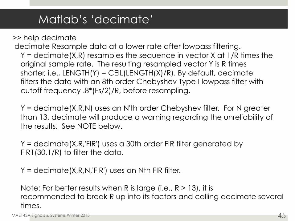
Matlab’s ‘decimate’
MAE143A Signals & Systems Winter 2015 45
>> help decimate decimate Resample data at a lower rate after lowpass filtering. Y = decimate(X,R) resamples the sequence in vector X at 1/R times the original sample rate. The resulting resampled vector Y is R times shorter, i.e., LENGTH(Y) = CEIL(LENGTH(X)/R). By default, decimate filters the data with an 8th order Chebyshev Type I lowpass filter with cutoff frequency .8*(Fs/2)/R, before resampling. Y = decimate(X,R,N) uses an N'th order Chebyshev filter. For N greater than 13, decimate will produce a warning regarding the unreliability of the results. See NOTE below. Y = decimate(X,R,'FIR') uses a 30th order FIR filter generated by FIR1(30,1/R) to filter the data. Y = decimate(X,R,N,'FIR') uses an Nth FIR filter. Note: For better results when R is large (i.e., R > 13), it is recommended to break R up into its factors and calling decimate several times.

Matlab’s ‘downsample’
Downsampling is asking for trouble with physical signals It is a common mistake made by people
It is not really forgivable though No graduate of MAE143A has ever admitted to me to making this mistake
MAE143A Signals & Systems Winter 2015 46
>> help downsample downsample Downsample input signal. downsample(X,N) downsamples input signal X by keeping every N-th sample starting with the first. If X is a matrix, the downsampling is done along the columns of X. downsample(X,N,PHASE) specifies an optional sample offset. PHASE must be an integer in the range [0, N-1].
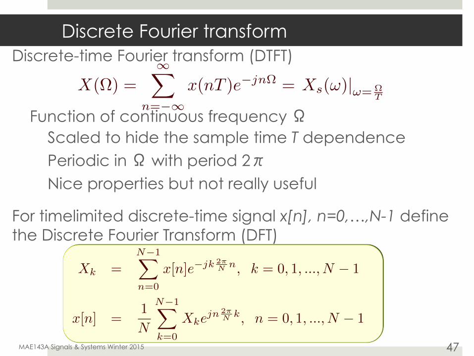
Discrete Fourier transform Discrete-time Fourier transform (DTFT)
Function of continuous frequency Ω
Scaled to hide the sample time T dependence Periodic in Ω with period 2π Nice properties but not really useful
For timelimited discrete-time signal x[n], n=0,…,N-1 define the Discrete Fourier Transform (DFT)
MAE143A Signals & Systems Winter 2015 47
X(⌦) =1X
n=�1x(nT )e�jn⌦ = Xs(!)|!=⌦
T
Xk =N�1X
n=0
x[n]e�jk 2⇡N n
, k = 0, 1, ..., N � 1
x[n] =1
N
N�1X
k=0
Xkejn 2⇡
N k, n = 0, 1, ..., N � 1

Discrete Fourier transform
DFT: N signal samples in and N transform values out Related to DTFT
Inverse DFT: N in values and N time samples out N is referred to as the record length If {x[n]} is real then
MAE143A Signals & Systems Winter 2015 48
Xk =N�1X
n=0
x[n]e�jk 2⇡N n
, k = 0, 1, ..., N � 1
x[n] =1
N
N�1X
k=0
Xkejn 2⇡
N k, n = 0, 1, ..., N � 1
Xk = X(⌦)|⌦= 2⇡kN
X�k = X̄k

Interpretation of the DFT
N-sample data record
Periodic repetition – forever What is the Fourier series?
Period of this repetition is NT
MAE143A Signals & Systems Winter 2015 49
{x0, x1, . . . , xN�1}x0
x1x2
xN�1
T 2T (N-1)T 0
time time
x0 x0x0
… … } } } }period NT period NT period NT period NT
xrep(t) =1X
k=�1cke
jk 2⇡NT t
ck =1
NT
Z NT�
0�xrep(t)e
�jk 2⇡NT t
dt
xrep(t) =
1X
n=�1x[n mod N ]�(t� nT )
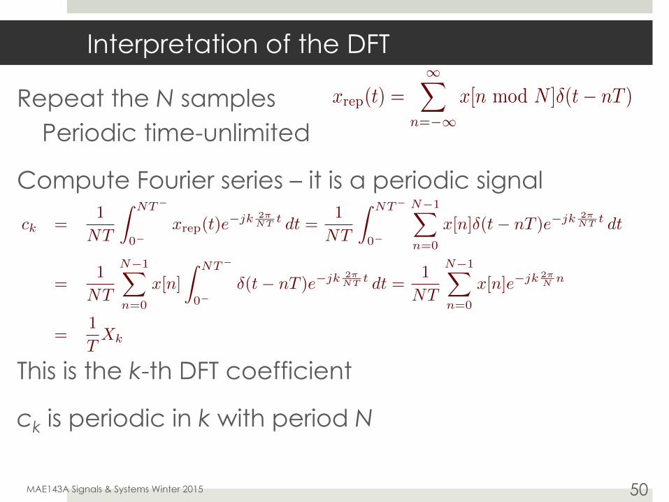
Interpretation of the DFT
Repeat the N samples Periodic time-unlimited
Compute Fourier series – it is a periodic signal
This is the k-th DFT coefficient
ck is periodic in k with period N
MAE143A Signals & Systems Winter 2015 50
xrep(t) =
1X
n=�1x[n mod N ]�(t� nT )
ck =1
NT
Z NT�
0�xrep(t)e
�jk 2⇡NT t
dt =1
NT
Z NT�
0�
N�1X
n=0
x[n]�(t� nT )e�jk 2⇡NT t
dt
=1
NT
N�1X
n=0
x[n]
Z NT�
0��(t� nT )e�jk 2⇡
NT tdt =
1
NT
N�1X
n=0
x[n]e�jk 2⇡N n
=1
T
Xk
The Discrete Fourier Transform
The DFT of an N-sample (real) signal record is an N element (complex) transform record is the Fourier series of the periodic (sampled) signal repeated over and over again in both directions is N-periodic in frequency bin (k)
We cannot resolve frequency more finely because there are only N data The frequency data have a conjugate relation Plotting |Xk| is a line spectrum as if the data were N-periodic
MAE143A Signals & Systems Winter 2015 51
X�k = X̄k

Sunspot example from the Kamen & Heck book
Go to: http://sidc.oma.be/index.php3 Monthly sunspot data since 1749
Edit the file to remove leading and trailing rows with ‘*’ or fewer columns than four
>> load spot.dat
>> spd=spot(1:300,3);
>> plot(1749+[1:300]/12,spd)
300 data points 25 years
Compute the DFT
MAE143A Signals & Systems Winter 2015 52
1750 1755 1760 1765 17700
20
40
60
80
100
120
140
160Sunspot data from Belgian Royal Observatory
year
num
ber

DFT of sunspot data
MAE143A Signals & Systems Winter 2015 53 0 50 100 150 200 250 300
0
2000
4000
6000
8000
10000
12000
14000
16000DFT magnitudes for 300 sunspot data
k
|Xk|
Note the symmetry about bin 150 Note strong dc component Note something at low frequencies
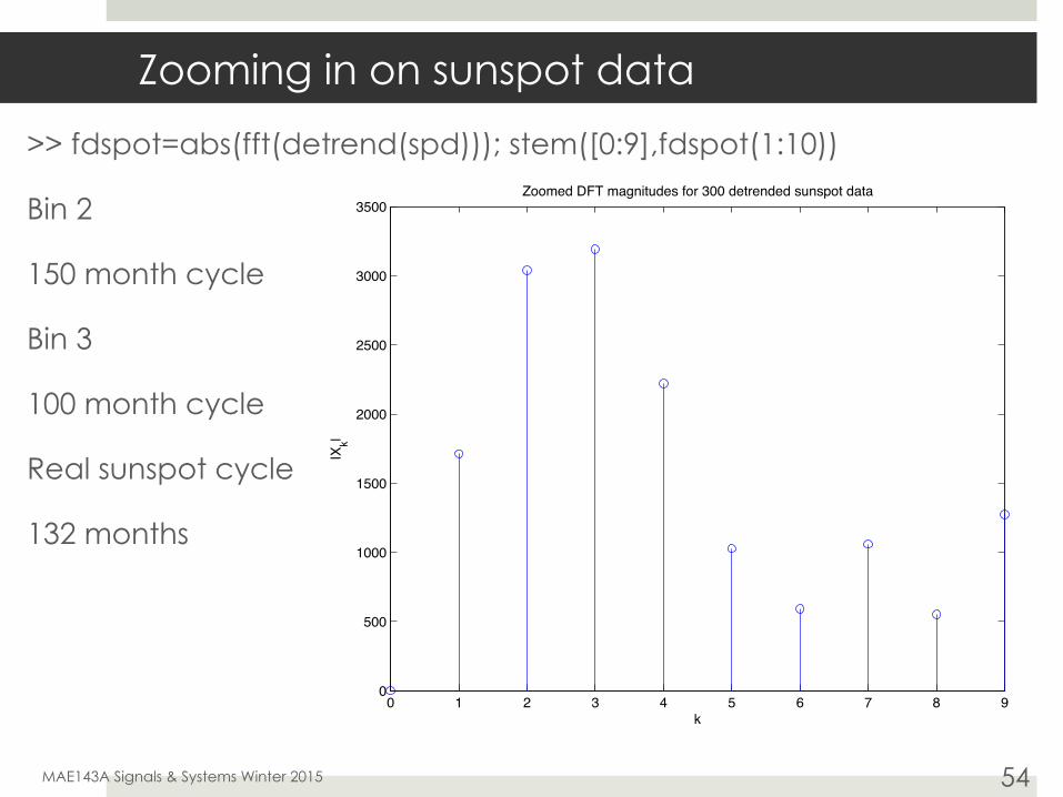
Zooming in on sunspot data
>> fdspot=abs(fft(detrend(spd))); stem([0:9],fdspot(1:10))
Bin 2
150 month cycle
Bin 3
100 month cycle
Real sunspot cycle
132 months
MAE143A Signals & Systems Winter 2015 54
0 1 2 3 4 5 6 7 8 90
500
1000
1500
2000
2500
3000
3500Zoomed DFT magnitudes for 300 detrended sunspot data
k
|Xk|
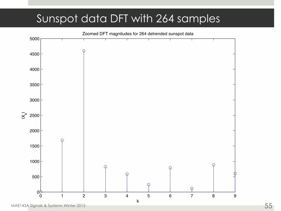
Sunspot data DFT with 264 samples
MAE143A Signals & Systems Winter 2015 55
0 1 2 3 4 5 6 7 8 90
500
1000
1500
2000
2500
3000
3500
4000
4500
5000Zoomed DFT magnitudes for 264 detrended sunspot data
k
|Xk|
DFT
The DFT allows analysis of a data record by computing the Fourier series as if the data record were one period of an infinite periodic sequence
This is good for capturing periodic phenomena in the data provided you have an integer number of periods in the data
It is easy to be misled Especially if you forget the above explanation
The DFT is a fundamental tool in data analysis There is a huge number of helper functions in matlab
MAE143A Signals & Systems Winter 2015 56


![Discrete Control - Real-Time Systems, Lecture 14 · Discrete Control Real ... System: Chapter 12] 1. Discrete Event Systems 2. ... mechanism is time-driven. Continuous discrete-time](https://img.dokumen.tips/doc/110x75/5b1497697f8b9a3e7c8daf88/discrete-control-real-time-systems-lecture-14-discrete-control-real-system.jpg)