Fourier Analysis D. Gordon E. Robertson, PhD, FCSB School of Human Kinetics University of Ottawa

Fourier AnalysisFourier Analysis

D. Gordon E. Robertson, PhD, FCSBD. Gordon E. Robertson, PhD, FCSB

School of Human Kinetics

University of Ottawa

04/19/2304/19/23Biomechanics Laborartory, Biomechanics Laborartory,

University of OttawaUniversity of Ottawa 22

In theory: Every periodic signal can be represented by a series (sometimes an infinite series) of sine waves of appropriate amplitude and frequency.

In practice: Any signal can be represented by a series of sine waves.

The series is called a Fourier series. The process of converting a signal to its Fourier

series is called a Fourier Transformation.

Why use Fourier Analysis?Why use Fourier Analysis?



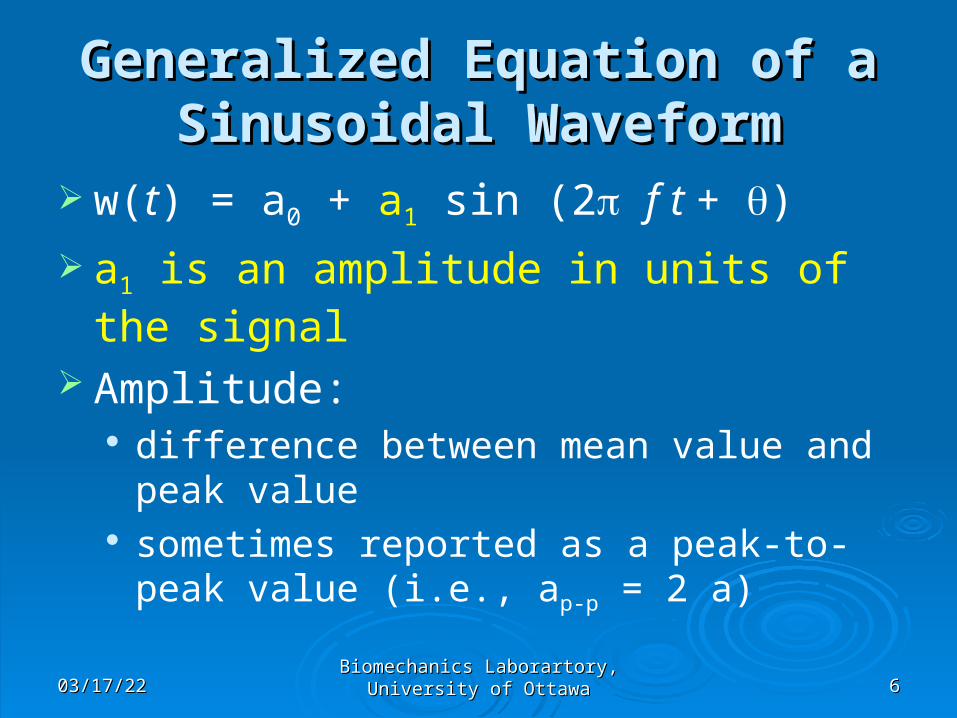
Generalized Equation of aGeneralized Equation of aSinusoidal WaveformSinusoidal Waveform

w(t) = a0 + a1 sin (2 f t + )

w(t) is the value of the waveform at time t




w(t) = a0 + a1 sin (2 f t + )

a0 is an offset in units of the signal

Offset (also called DC level or DC bias): mean value of the signal AC signals, such as the line voltage of an

electrical outlet, have means of zero



Offset ChangesOffset Changes

offset > 0

offset < 0

zero

zero

zero

offset = 0




w(t) = a0 + a1 sin (2 f t + )

a1 is an amplitude in units of the signal

Amplitude: difference between mean value and peak

value sometimes reported as a peak-to-peak value

(i.e., ap-p = 2 a)



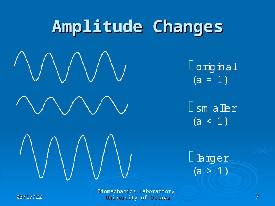
Amplitude ChangesAmplitude Changes

smaller (a < 1)

larger (a > 1)

original (a = 1)




w(t) = a0 + a1 sin (2 f t + ) f is the frequency in cycles per second or

hertz (Hz) Frequency:

number of cycles (n) per second sometimes reported in radians per second

(i.e., = 2 f ) can be computed from duration of the cycle or

period (T): (f = n/T)



Frequency ChangesFrequency Changes

original (f = 1)

faster (f > 1)

slower (f < 1)




w(t) = a0 + a1 sin (2 f t + )

is phase angle in radians Phase angle:

delay or phase shift of the signal can also be reported as a time delay in

seconds e.g., if , sine wave becomes a cosine



Phase ChangesPhase Changes

delayed (lag, > 0)

early (lead, < 0)

zero time

original ( = 0)



Generalized Equation of aGeneralized Equation of a Fourier Series Fourier Series

w(t) = a0 + ai sin (2 fi t + i)

since frequencies are measured in cycles per second and a cycle is equal to 2 radians, the frequency in radians per second, called the angular frequency, is:

= 2 f therefore:

w(t) = a0 + ai sin (i t + i)



Alternate Form of Fourier Alternate Form of Fourier TransformTransform

an alternate representation of a Fourier series uses sine and cosine functions and harmonics (multiples) of the fundamental frequency

the fundamental frequency is equal to the inverse of the period (T, duration of the signal): f1 = 1/period = 1/T

phase angle is replaced by a cosine function maximum number in series is half the number of

data points (number samples/2)



Fourier CoefficientsFourier Coefficients

w(t) = a0 + [ bi sin (i t) + ci cos (i t) ] bi and ci, called the Fourier coefficients, are the

amplitudes of the paired series of sine and cosine waves (i=1 to n/2); a0 is the DC offset

various processes compute these coefficients, such as the Discrete Fourier Transform (DFT) and the Fast Fourier Transform (FFT)

FFTs compute faster but require that the number of samples in a signal be a power of 2 (e.g., 512, 1024, 2048 samples, etc.)



Fourier Transforms of Known Fourier Transforms of Known WaveformsWaveforms

Sine wave:w(t)=a sin(wt)

Square wave:w(t)=a [sin(t) + 1/3 sin(3t) + 1/5 sin(5t) + ... ]

Triangle wave:w(t)=8a/2 [cos(t) + 1/9 cos(3t) + 1/25 cos(5t) + ...]

Sawtooth wave:w(t)=2a/ [sin(t) – 1/2 sin(2t) + 1/3 sin(3t)

– 1/4 sin(4t) + 1/5 sin(5t) + ...]



Pezzack’s Angular Displacement Pezzack’s Angular Displacement DataData



Fourier Analysis of Pezzack’s Fourier Analysis of Pezzack’s Angular Displacement DataAngular Displacement Data

Bias = a0 = 1.0055 Harmonic Freq. ci bi Normalizednumber (hertz) cos() sin() power

1 0.353 -0.5098 0.3975 100.00002 0.706 -0.5274 -0.3321 92.94413 1.059 0.0961 0.2401 16.00554 1.411 0.1607 -0.0460 6.68745 1.764 -0.0485 -0.1124 3.58496 2.117 -0.0598 0.0352 1.15227 2.470 0.0344 0.0229 0.40808 2.823 0.0052 -0.0222 0.12429 3.176 -0.0138 0.0031 0.048110 3.528 0.0051 0.0090 0.025811 3.881 -0.0009 -0.0043 0.0045



Reconstruction of Pezzack’s Reconstruction of Pezzack’s Angular Displacement DataAngular Displacement Data

raw signal (green)8 harmonics (cyan)4 harmonics (red)2 harmonics (magenta)

8 harmonics gave a reasonable approximation

Documents

Fourier Analysis D. Gordon E. Robertson, PhD, FCSB School of Human Kinetics University of Ottawa