Four-wheel Driving-force Distribution Method for ...hflab.k.u-tokyo.ac.jp/papers/2013/maedaAUTOMATIKA13.pdf · Four-wheel Driving-force Distribution Method for Instantaneous or Split

Kenta Maeda, Hiroshi Fujimoto, Yoichi Hori

Four-wheel Driving-force Distribution Methodfor Instantaneous or Split Slippery Roads for Electric Vehicle

In this paper, a four-wheel driving force distribution method based on driving force control is proposed. Drivingforce control is an anti-slip control method, previously proposed by the authors’ research group, which generatesappropriate driving force based on the acceleration pedal. However, this control method cannot completely preventreduction of driving force when a vehicle runs on an extremely slippery road. If the length of a slippery surfaceis shorter than the vehicle’s wheel base, the total driving force is retained by distributing the shortage of drivingforce to the wheels that still have traction. On the other hand, when either the left or right side runs on a slipperysurface, yaw-moment is suppressed by setting total driving forces of left and right wheels to be the same. Therefore,four-wheel driving force distribution method is proposed for retaining driving force on instantaneous slippery roads,and suppressing yaw-moment on split ones. The effectiveness of the proposed distribution method is verified bysimulations and experiments.

Key words: Electric vehicle, Traction control, Slip ratio, Driving force, Least squares method

Metoda za raspodjelu pogonske sile elektricnih vozila sa cetiri kotaca na kratkotrajno ili polovicnoskliskim cestama. U ovom radu predložena je metoda za raspodjelu pogonske sile elektricnih vozila sa cetirikotaca temeljena na upravljanju pogonskom silom. Upravljanje pogonskom silom je metoda upravljanja koju jeranije predložila autorova istraživacka grupa, a koristi se za sprjecavanje proklizavanja. Ova metoda generira prik-ladnu pogonsku silu temeljem pritiska na papucicu ubrzanja. Ipak, ova metoda upravljanja ne može u potpunostisprijeciti smanjenje pogonske sile kada vozilo nai�e na ekstremno sklisku cestu. Ako je dužina skliske površinekraca od me�uosovinskog razmaka vozila, ukupna pogonska sila se zadržava redistribucijom manjka pogonske silena kotace koji i dalje imaju trakciju. S druge strane, kada lijeva ili desna strana vozila nai�e na sklisku površinu,moment zakretanja se potiskuje postavljanjem ukupne pogonske sile lijevih i desnih kotaca na jednaki iznos. Dakle,metoda za raspodjelu pogonske sile predložena je za zadržavanje pogonske sile na kratkotrajno skliskim cestama, teza sprjecavanje momenta zakretanja na polovicno skliskim cestama. Ucinkovitost predložene metode verificiranaje simulacijski i eksperimentalno.

Kljucne rijeci: elektricno vozilo, upravljanje proklizavanjem, omjer proklizavanja, pogonska sila, metoda najman-jih kvadrata

1 INTRODUCTIONAs a solution for energy and environmental problems,

electric vehicles (EVs) have been receiving great attention.In addition, EVs have many advantages over internal com-bustion engine vehicles, since electric motors and invertersare utilized in EV drive systems. Their advantages can besummarized as follows [1]:

1. The torque response of electric motors is 10–100times faster than that of engines.

2. All wheels can be controlled independently by adopt-ing small high-power in-wheel motors.

3. The output torque of an electric motor can be mea-sured accurately from the motor current.

Based on these advantages, many traction control meth-ods for anti-skid on slippery surface have been proposed.These methods are based on torque observer [2, 3], max-imum transmissible torque estimation [4], slip ratio con-trol [5, 6], sliding mode control [7] and so on. In addition,since the road friction coefficient µ decides the maximumtorque that a wheel can generate on the surface, estimationmethods of the µ have been proposed [8–10].

Four-wheel Driving-force Distribution Method for Instantaneous or Split Slippery Roads for Electric Vehicle K. Maeda, H. Fujimoto, Y. Hori

The authors’ research group also has proposed trac-tion control methods [11–14]. Driving force control (DFC)[11], the latest one, is a control method that directly con-trols driving force with driving force outer loop based ondriving force observer, and wheel-speed inner loop basedon slip ratio control [12, 13], which can generate large yetuncertain driving force on slippery roads. With this con-trol system, the desired driving force is generated withinthe saturator limits, and traction is retained by slip ratiocontrol when the driving force saturates. Moreover, driv-ing force commanded by a driver can be generated by usingthe acceleration pedal as the driving force reference.

Since DFC proposed in [11] is considered for front-wheel-driven EVs, it is inevitable that total driving forcediminishes on extremely slippery roads, which also appliesto the other traction control methods. However, suddendecrease of driving force leads to driver discomfort, andthus a novel control method is needed to retain total drivingforce. In addition, the left and right driving forces need tobe equal to prevent yawing.

In this paper, a four-wheel driving force distributionmethod based on DFC is proposed for EV with in-wheelmotors. As mentioned, it is one of EVs’ advantages thatall-wheel-drive vehicles can easily be realized by adopt-ing small high-power in-wheel motors. Even when a ve-hicle runs into a slippery road such as scattered snow orwet manholes, whose length is shorter than the vehicle’swheel base, total driving force is retained by distributingthe shortage of driving force to wheels that still have trac-tion. Additionally, when either left or right side are on aslippery surface, yaw motion is suppressed by generatingthe difference between left and right driving force to followdesired yaw-moment — zero when running straight. Thefour-wheel driving force distribution method proposed inthis paper can realize both functions simultaneously. Theeffectiveness of the proposed method is verified by simu-lations and experiments.

2 EXPERIMENTAL VEHICLE AND VEHICLEMODEL

2.1 Experimental VehicleThe experimental EV “FPEV2-Kanon,” developed by

the authors’ laboratory, is used for performance verifica-tion as shown in Fig. 1. In this section the characteristicsof the experimental vehicle are explained.

Outer-rotor-type in-wheel motors shown in Fig. 2 areinstalled in each wheel. Since these motors adopt directdrive system, reaction forces from the road are directlytransferred to the motors without gear reduction or back-lash. The maximum torque of each of the front motorsis ±500 [Nm], and that of the rear is ±340 [Nm]. Addi-tionally, an optical sensor is installed to measure the vehi-

Fig. 1. FPEV2-Kanon. Fig. 2. In-wheel mo-tor.

Table 1. Vehicle specifications.Vehicle Mass (m) 870 [kg]

Wheel Base (l) 1.7 [m]Distance from C.G to Front Axle (lf ) 0.999 [m]Distance from C.G to Rear Axle (lr) 0.701 [m]

Tread Base (df , dr) 1.3 [m]Wheel Radius (r) 0.302 [m]

cle velocity accurately. The vehicle’s specification is ex-pressed in Table 1.

2.2 Equations of Vehicle Dynamics

In this section, equations of vehicle dynamics are ex-plained [11].

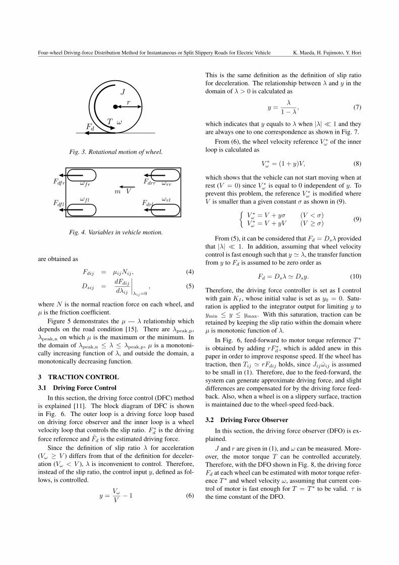
The equation of rotational motion of each wheel (asshown in Fig. 3) can be described as

Jijωij = Tij − rFdij , (1)

where J is the wheel inertia, ω is the wheel angular ve-locity, T is the motor torque, r is the wheel radius, Fd isthe driving force at the point where the wheel makes con-tact with the ground. Also, i and j are indices for f/r(front/rear) and l/r (left/right) respectively.

The equation of longitudinal motion of the vehiclebody (as shown in Fig. 4) can be described as

mV = Fdfl + Fdfr + Fdrl + Fdrr, (2)

where m is the vehicle mass, V is the vehicle velocity.

When the vehicle accelerates or decelerates, the wheelvelocity Vω = rω differs from the vehicle velocity V be-cause of tire’s elastic deformation. Therefore the slip ratioλ is defined as

λ =Vω − V

max(Vω, V, ϵ), (3)

where ϵ is a tiny value to prevent division by zero. Thedriving force Fd and the driving stiffness Ds at each wheel


ωT

r

Fd

J

Fig. 3. Rotational motion of wheel.

m V

Fdfr

Fdfl

Fdrr

Fdrl

ωfr

ωfl

ωrr

ωrl

Fig. 4. Variables in vehicle motion.

are obtained as

Fdij = µijNij , (4)

Dsij =dFdij

dλij

∣∣∣∣λij=0

, (5)

where N is the normal reaction force on each wheel, andµ is the friction coefficient.

Figure 5 demonstrates the µ — λ relationship whichdepends on the road condition [15]. There are λpeak,p,λpeak,n on which µ is the maximum or the minimum. Inthe domain of λpeak,n ≤ λ ≤ λpeak,p, µ is a monotoni-cally increasing function of λ, and outside the domain, amonotonically decreasing function.

3 TRACTION CONTROL3.1 Driving Force Control

In this section, the driving force control (DFC) methodis explained [11]. The block diagram of DFC is shownin Fig. 6. The outer loop is a driving force loop basedon driving force observer and the inner loop is a wheelvelocity loop that controls the slip ratio. F ∗

d is the drivingforce reference and Fd is the estimated driving force.

Since the definition of slip ratio λ for acceleration(Vω ≥ V ) differs from that of the definition for deceler-ation (Vω < V ), λ is inconvenient to control. Therefore,instead of the slip ratio, the control input y, defined as fol-lows, is controlled.

y =Vω

V− 1 (6)

This is the same definition as the definition of slip ratiofor deceleration. The relationship between λ and y in thedomain of λ > 0 is calculated as

y =λ

1− λ, (7)

which indicates that y equals to λ when |λ| ≪ 1 and theyare always one to one correspondence as shown in Fig. 7.

From (6), the wheel velocity reference V ∗ω of the inner

loop is calculated as

V ∗ω = (1 + y)V, (8)

which shows that the vehicle can not start moving when atrest (V = 0) since V ∗

ω is equal to 0 independent of y. Toprevent this problem, the reference V ∗

ω is modified whereV is smaller than a given constant σ as shown in (9).{

V ∗ω = V + yσ (V < σ)

V ∗ω = V + yV (V ≥ σ)

(9)

From (5), it can be considered that Fd = Dsλ providedthat |λ| ≪ 1. In addition, assuming that wheel velocitycontrol is fast enough such that y ≃ λ, the transfer functionfrom y to Fd is assumed to be zero order as

Fd = Dsλ ≃ Dsy. (10)

Therefore, the driving force controller is set as I controlwith gain KI , whose initial value is set as y0 = 0. Satu-ration is applied to the integrator output for limiting y toymin ≤ y ≤ ymax. With this saturation, traction can beretained by keeping the slip ratio within the domain whereµ is monotonic function of λ.

In Fig. 6, feed-forward to motor torque reference T ∗

is obtained by adding rF ∗d , which is added anew in this

paper in order to improve response speed. If the wheel hastraction, then Tij ≃ rFdij holds, since Jijωij is assumedto be small in (1). Therefore, due to the feed-forward, thesystem can generate approximate driving force, and slightdifferences are compensated for by the driving force feed-back. Also, when a wheel is on a slippery surface, tractionis maintained due to the wheel-speed feed-back.

3.2 Driving Force Observer

In this section, the driving force observer (DFO) is ex-plained.

J and r are given in (1), and ω can be measured. More-over, the motor torque T can be controlled accurately.Therefore, with the DFO shown in Fig. 8, the driving forceFd at each wheel can be estimated with motor torque refer-ence T ∗ and wheel velocity ω, assuming that current con-trol of motor is fast enough for T = T ∗ to be valid. τ isthe time constant of the DFO.


−1 −0.5 0 0.5 1

−0.2

−0.1

0

0.1

0.2

0.3

slip ratio λ

fric

tion

coef

ficie

nt µ

λpeak,p

λpeak,n

Fig. 5. Typical µ-λ relationship.

y

1y + 1

PIVehicle

Plant

Wheel Speed Control

Driving Force Control

Driving Force Observer

+

−

F∗

d 1s

V

ω

Js1

τs+1

T∗

ω∗

V∗

ωKI

Fd

+ −

+

++

+

+

−

1r

1r

rFeed-forward

1τs+1

Fig. 6. Block diagram of DFC.

−0.2 −0.1 0 0.1 0.2−0.2

−0.1

0

0.1

0.2

0.3

slip ratio λ

y

Fig. 7. The relationship between λ and y.

rFd

1

Js

ω

Js

1

τs+1

1

r

T

Fd

+ −

+ −

Fig. 8. Block diagram of driving force observer.

4 PROPOSED METHOD

4.1 Driving Force Distribution Method

In this section, four-wheel driving force distribution isexplained. When slip ratio λ increases on a slippery sur-face and the control input y of DFC approaches the upperlimit, driving force is saturated and reduced. To avoid thisreduction, λ of each wheel need to be small enough to pre-vent saturation. Therefore, the proposed method decidesthe driving force reference F ∗

dij of each wheel to minimizeλij of each wheel, satisfying total driving force referenceF ∗dall and yaw-moment reference M∗

z generated by drivingforce difference between left and right.

The relationship between driving force of each wheelFdij and Fdall, Mz is as follows:

[1 1 1 1

−df

2df

2 −dr

2dr

2

]Fdfl

Fdfr

Fdrl

Fdrr

=

[Fdall

Mz

].

(11)Here, by setting the coefficient matrix in the left-handside as A, the vector of driving force of each wheel[Fdfl, Fdfr, Fdrl, Fdrr]

T as x, and that of total driving

force and yaw-moment [Fdall,Mz]T as b, (11) can be

rewritten as Ax = b. From (10) driving stiffness of eachwheel Dsij in the domain of |λ| ≪ 1 can be obtained as

Dsij =Fdij

λij. (12)

Then the cost function J is defined as the sum of squaresof slip ratio λij .

J = λ2fl + λ2

fr + λ2rl + λ2

rr

=F 2dfl

D2sfl

+F 2dfr

D2sfr

+F 2drl

D2srl

+F 2drr

D2srr

(13)

Therefore, the weighted least squares solution xopt of (11)that minimizes J , and weighting matrix W are as follows.

xopt = W−1AT (AW−1AT )−1b (14)

W = diag

(1

D2sfl

,1

D2sfr

,ϕr

D2srl

,ϕr

D2srr

)(15)

Here, ϕr is the tuning gain which adjust front and rear driv-ing force distribution ratio. Larger amount of driving force


WeightedLeastSquaresMethod

DFC

DFC

DFC

DFC

Vehicle

DFORecursiveLeast SquaresMethod

ωfl

ωfr

ωrl

ωrr

T∗

fl

T∗

fr

T∗

rl

T∗

rr

Fdrl,Fdrr

Dsfl,Dsfr

Dsrl,Dsrr

F∗

dall

M∗

z

F∗

dfl

F∗

dfr

F∗

drl

F∗

drr V

Slip RatioCalculationλfl,λfr,λrl,λrr

Fdfl,Fdfr

Fig. 9. Block diagram of the proposed method.

FPEV2-Kanon

low-µsheet

0.9m

4.0m

start point

2.0m

Fig. 10. Instantaneous low-µ road.

FPEV2-Kanonlow-µsheet

0.9m

2.0m

start point

2.0m

Fig. 11. Split low-µ road.

is distributed to rear wheels than front ones during acceler-ation, which possibly leads to excessive driving force ref-erences on rear wheels over the upper limit of rear motortorque and total driving force saturates even on a high-µsurface. Therefore ϕr is set as ϕr ≥ 1 during accelerationto prevent the saturation.

4.2 Driving Stiffness Estimation

From (12), the relationship between Fd and λ is Fd =Dsλ. Therefore the driving stiffness of each wheel at sam-ple k Dsij(k) can be estimated by the Recursive LeastSquares (RLS) Method as follows [14].

Dsij(k) = Dsij(k − 1)− Γ(k − 1)λ(k)

w + λij(k)Γ(k − 1)λij(k)

×[λij(k)Dsij(k − 1)− Fdij(k)

](16)

Γ(k) =1

w

[Γ(k − 1)− Γ(k − 1)λij(k)

2Γ(k − 1)

w + λij(k)Γ(k − 1)λij(k)

](17)

where w is the forgetting factor. If regressor λij(k) equalszero, the persistent excitation is not satisfied. Therefore

Dsij(k) and Γ(k) are not updated if |λij(k)| < 0.005.Lower limitations 1000 are imposed to Dsij avoiding divi-sion by zero in (15).

Figure 9 shows the block diagram of the whole system.The driving force references F ∗

dij are given by xopt.

5 SIMULATION

5.1 Simulation Setup

In this section, simulation results of acceleration testare explained. In this paper, “2D-Tire Model” [16] is usedfor vehicle running simulation.

As shown in Fig. 10 and Fig. 11, an extremely lowµ (µ = 0.15) surface of length 0.9 [m], shorter than thewheel base of “FPEV2-Kanon", is set at the distance of2.0 [m] from the start point. The experimental vehiclestarts at the start point and accelerates with total drivingforce reference F ∗

dall = 2000 [N].

The parameters are, KI = 0.01, τ = 30 [ms], ymax =0.25 which corresponds to a slip ratio of λ = 0.2, σ =0.5 [m/s]. The wheel speed PI controller is designed bythe pole assignment method towards the plant 1

Js , which


0 0.5 1 1.5 2 2.5 3 3.50

0.2

0.4

0.6

0.8

time [s]

slip

rat

io [−

]

FLFRRLRR

(a) λ on each wheel.

0 0.5 1 1.5 2 2.5 3 3.50

200

400

600

800

1000

time [s]

driv

ing

forc

e [N

]

FLFRRLRR

(b) Fd on each wheel.

0 0.5 1 1.5 2 2.5 3 3.50

500

1000

1500

2000

2500

3000

time [s]

tota

l driv

ing

forc

e [N

]

Fdall

reference

(c) Fdall.

Fig. 12. Simulation of instantaneous slippery road (without control).

0 0.5 1 1.5 2 2.5 3 3.50

0.05

0.1

0.15

0.2

0.25

time [s]

slip

rat

io [−

]

FLFRRLRR


0 0.5 1 1.5 2 2.5 3 3.50

200

400

600

800

1000

time [s]

driv

ing

forc

e [N

]

FLFRRLRR


0 0.5 1 1.5 2 2.5 3 3.50

500

1000

1500

2000

2500

3000

time [s]

tota

l driv

ing

forc

e [N

]

Fdall

reference

(c) Fdall.

0 0.5 1 1.5 2 2.5 3 3.50

0.05

0.1

0.15

0.2

0.25

time [s]

y

FLFRRLRR

(d) y on each wheel.

Fig. 13. Simulation of instantaneous slippery road (only DFC).

0 0.5 1 1.5 2 2.5 3 3.50

0.05

0.1

0.15

0.2

0.25

time [s]

slip

rat

io [−

]

FLFRRLRR


0 0.5 1 1.5 2 2.5 3 3.50

200

400

600

800

1000

time [s]

driv

ing

forc

e [N

]

FLFRRLRR


0 0.5 1 1.5 2 2.5 3 3.50

500

1000

1500

2000

2500

3000

time [s]

tota

l driv

ing

forc

e [N

]

F

dall

reference

(c) Fdall.

0 0.5 1 1.5 2 2.5 3 3.50

0.05

0.1

0.15

0.2

0.25

time [s]

y

FLFRRLRR


Fig. 14. Simulation of instantaneous slippery road (proposed).

is from (1) ignoring Fd, setting the pole −20 [rad/s]. Theforgetting factor of the driving stiffness estimation is w =0.995. All parameters are the same for each wheel.

5.2 Instantaneous Slippery RoadFigures 12 – 14 show the simulation results of acceler-

ation test on instantaneous slippery surface. In each result,front wheels are on slippery surface from about 1.8 [s] to2.1 [s], and rear ones are from about 2.3 [s] to 2.5 [s].

The simulation results are compared with three con-ditions. Figure 12 shows the results of acceleration testwithout any traction control, i.e., motor torque on eachwheel is set as 500r = 151 [Nm] constantly. Then Fig.13 shows the results of the conventional method with onlyDFC and without driving force distribution, i.e., drivingforce references on each wheel are the same. Finally Fig.

14 shows the results of the proposed method with DFC andthe driving-force distribution.

In case without control, extreme slip occurs in Fig.12(a) then the driving force decreases in Fig. 12(b), 12(c).In case with only DFC, although the traction is obtained inFig. 13(a), the driving force decreases in Fig. 13(b), 13(c),similar to the case without control.

On the contrary, with the proposed method, Fig. 14(b)shows that the driving force on each wheel is distributedto retain total driving force as shown in Fig. 14(c), as wellas the traction shown in Fig. 14(a). In addition, comparedto Fig. 13(d), Fig. 14(d) shows that the proposed methodprevents the satulation of the DFC control input y.

In Fig. 14(c), the total driving force is not completelyretained and slightly decreases from the reference whenfront wheels are on the slippery surface. This is because


0 0.5 1 1.5 2 2.5 3 3.50

200

400

600

800

1000

time [s]

driv

ing

forc

e [N

]

FLFRRLRR

(a) Fd on each wheel.

0 0.5 1 1.5 2 2.5 3 3.50

500

1000

1500

2000

2500

3000

time [s]

tota

l driv

ing

forc

e [N

]

F

dall

reference

(b) Fdall.

0 0.5 1 1.5 2 2.5 3 3.5−300

−200

−100

0

100

200

300

time [s]

yaw

−m

omen

t [N

m]

(c) Mz .

0 0.5 1 1.5 2 2.5 3 3.50

0.05

0.1

0.15

0.2

0.25

time [s]

y

FLFRRLRR


Fig. 15. Simulation of split slippery road (only DFC).

0 0.5 1 1.5 2 2.5 3 3.50

200

400

600

800

1000

time [s]

driv

ing

forc

e [N

]

FLFRRLRR


0 0.5 1 1.5 2 2.5 3 3.50

500

1000

1500

2000

2500

3000

time [s]

tota

l driv

ing

forc

e [N

]

F

dall

reference

(b) Fdall.

0 0.5 1 1.5 2 2.5 3 3.5−300

−200

−100

0

100

200

300

time [s]

yaw

−m

omen

t [N

m]

(c) Mz .

0 0.5 1 1.5 2 2.5 3 3.50

0.05

0.1

0.15

0.2

0.25

time [s]

y

FLFRRLRR


Fig. 16. Simulation of split slippery road (proposed).

the rear motor torque approaches to the upper limit andtherefore the rear driving forces are saturated.

5.3 Split Slippery Road

Figures 15 and 16 show the simulation results of ac-celeration test on split slippery surface. In each result,front-right wheel is on slippery surface from about 1.8 [s]to 2.1 [s], and rear-right one is from about 2.3 [s] to 2.5 [s].

Since the traction of DFC is indicated in the previoussection, result of acceleration test without control is ex-cluded. In case with only DFC, Fig. 15(a) shows that thedriving forces in only the right wheels reduce. As a result,the total driving force decreases as shown in Fig. 15(b),and the undesired yaw-moment is generated as shown inFig. 15(c). In contrast, with the proposed method, drivingforce of each wheel is distributed as shown in Fig. 16(a)to retain driving force while preventing the generation ofyaw-moment, which can be confirmed by comparing Fig.15(b), 15(c) with Fig. 16(b), 16(c). In addition, comparedto Fig. 15(d), Fig. 16(d) shows that the proposed methodprevents the saturation of y.

6 EXPERIMENTS

6.1 Experimental Setup

In this section, experimental results on an instantaneousslippery road are explained under the same condition asthe simulation in Section 5. A polymer sheet is utilized to

simulate slippery road condition. This sheet, called “low-µsheet" in this paper, can realize a friction coefficient µ ofabout 0.2 by watering on it. The control parameters are assame as simulation, while tuning gain of the driving forcedistribution is set as ϕr = 1.3.

Vehicle velocity is measured using an optical sensor.Since it can not measure velocity accurately on low speed,the slip ratio of each experimental result before 1.2 [s] isnot correct.

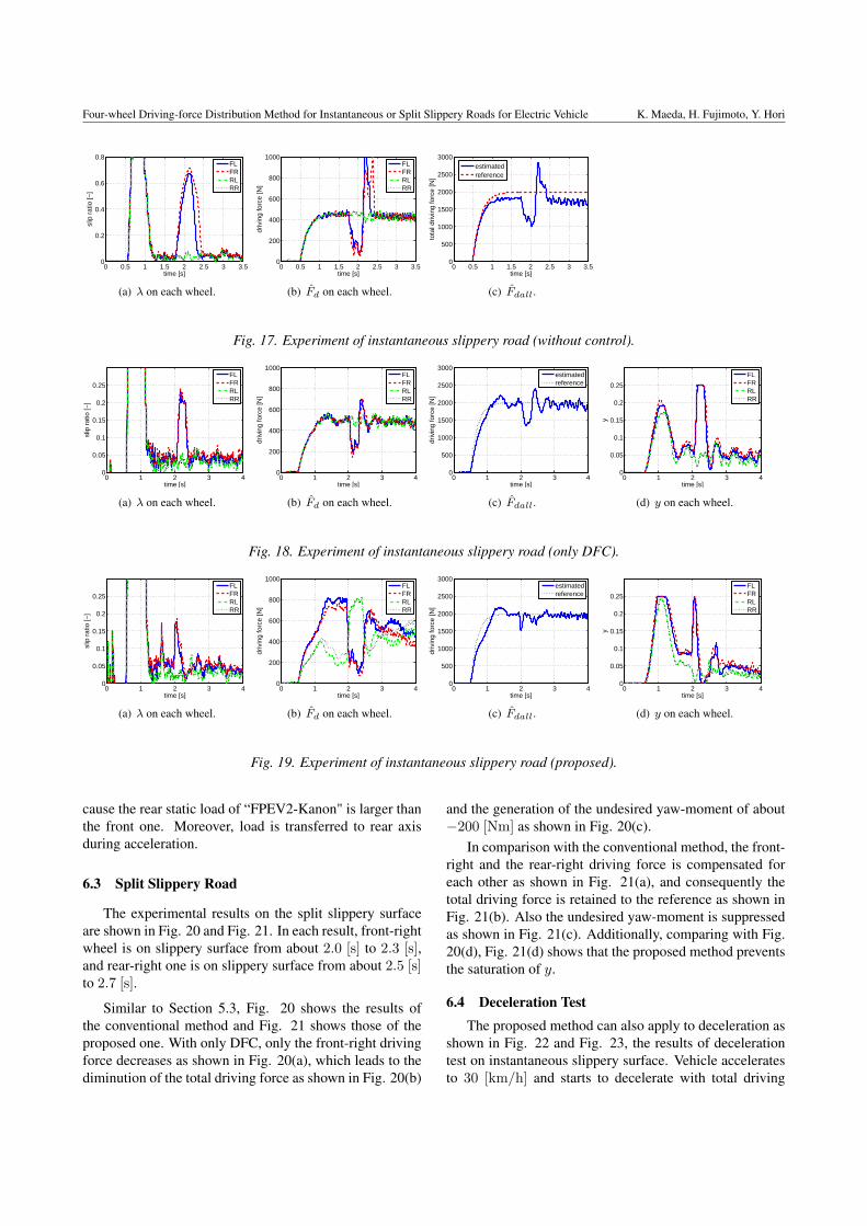
6.2 Instantaneous Slippery RoadThe experimental results are shown in Fig. 17–19. Re-

sults are compared with three cases as explained in Section5.2. In each result, front wheels are on slippery surfacefrom about 2.0 [s] to 2.3 [s], and rear ones are on slipperysurface from about 2.5 [s] to 2.7 [s].

Comparing Fig. 17(a) with Fig. 18(a) and 19(a), trac-tion is obtained by DFC. As for driving force, without con-trol and with only DFC, driving force decreases in Fig.17(b), Fig. 17(c), Fig. 18(b), Fig. 18(c), similar to thesimulation results. In contrast, with the proposed method,Fig. 19(b) shows that driving force on each wheel is dis-tributed to retain total driving force as shown in Fig. 19(c).Additionally, comparing with Fig. 18(d), Fig. 19(d) showsthat the proposed method prevents the saturation of y whenthe front wheels are on the slippery road.

Rear wheels do not reduce their driving force by theconventional method as shown in Fig. 18(b). This is be-


0 0.5 1 1.5 2 2.5 3 3.50

0.2

0.4

0.6

0.8

time [s]

slip

rat

io [−

]

FLFRRLRR


0 0.5 1 1.5 2 2.5 3 3.50

200

400

600

800

1000

time [s]

driv

ing

forc

e [N

]

FLFRRLRR


0 0.5 1 1.5 2 2.5 3 3.50

500

1000

1500

2000

2500

3000

time [s]

tota

l driv

ing

forc

e [N

]

estimatedreference

(c) Fdall.

Fig. 17. Experiment of instantaneous slippery road (without control).

0 1 2 3 40

0.05

0.1

0.15

0.2

0.25

time [s]

slip

rat

io [−

]

FLFRRLRR


0 1 2 3 40

200

400

600

800

1000

time [s]

driv

ing

forc

e [N

]

FLFRRLRR


0 1 2 3 40

500

1000

1500

2000

2500

3000

time [s]

driv

ing

forc

e [N

]

estimatedreference

(c) Fdall.

0 1 2 3 40

0.05

0.1

0.15

0.2

0.25

time [s]

y

FLFRRLRR


Fig. 18. Experiment of instantaneous slippery road (only DFC).

0 1 2 3 40

0.05

0.1

0.15

0.2

0.25

time [s]

slip

rat

io [−

]

FLFRRLRR


0 1 2 3 40

200

400

600

800

1000

time [s]

driv

ing

forc

e [N

]

FLFRRLRR


0 1 2 3 40

500

1000

1500

2000

2500

3000

time [s]

driv

ing

forc

e [N

]

estimatedreference

(c) Fdall.

0 1 2 3 40

0.05

0.1

0.15

0.2

0.25

time [s]

y

FLFRRLRR


Fig. 19. Experiment of instantaneous slippery road (proposed).

cause the rear static load of “FPEV2-Kanon" is larger thanthe front one. Moreover, load is transferred to rear axisduring acceleration.

6.3 Split Slippery Road

The experimental results on the split slippery surfaceare shown in Fig. 20 and Fig. 21. In each result, front-rightwheel is on slippery surface from about 2.0 [s] to 2.3 [s],and rear-right one is on slippery surface from about 2.5 [s]to 2.7 [s].

Similar to Section 5.3, Fig. 20 shows the results ofthe conventional method and Fig. 21 shows those of theproposed one. With only DFC, only the front-right drivingforce decreases as shown in Fig. 20(a), which leads to thediminution of the total driving force as shown in Fig. 20(b)

and the generation of the undesired yaw-moment of about−200 [Nm] as shown in Fig. 20(c).

In comparison with the conventional method, the front-right and the rear-right driving force is compensated foreach other as shown in Fig. 21(a), and consequently thetotal driving force is retained to the reference as shown inFig. 21(b). Also the undesired yaw-moment is suppressedas shown in Fig. 21(c). Additionally, comparing with Fig.20(d), Fig. 21(d) shows that the proposed method preventsthe saturation of y.

6.4 Deceleration TestThe proposed method can also apply to deceleration as

shown in Fig. 22 and Fig. 23, the results of decelerationtest on instantaneous slippery surface. Vehicle acceleratesto 30 [km/h] and starts to decelerate with total driving


0 1 2 3 40

200

400

600

800

1000

time [s]

driv

ing

forc

e [N

]

FLFRRLRR


0 1 2 3 40

500

1000

1500

2000

2500

3000

time [s]

driv

ing

forc

e [N

]

estimatedreference

(b) Fdall.

0 1 2 3 4−300

−200

−100

0

100

200

time [s]

yaw

−m

omen

t [N

m]

estimatedreference

(c) Mz .

0 1 2 3 40

0.05

0.1

0.15

0.2

0.25

time [s]

y

FLFRRLRR


Fig. 20. Experiment of split slippery road (only DFC).

0 1 2 3 40

200

400

600

800

1000

time [s]

driv

ing

forc

e [N

]

FLFRRLRR


0 1 2 3 40

500

1000

1500

2000

2500

3000

time [s]

driv

ing

forc

e [N

]

estimatedreference

(b) Fdall.

0 1 2 3 4−300

−200

−100

0

100

200

time [s]

yaw

−m

omen

t [N

m]

estimatedreference

(c) Mz .

0 1 2 3 40

0.05

0.1

0.15

0.2

0.25

time [s]

y

FLFRRLRR


Fig. 21. Experiment of split slippery road (proposed).

0 1 2 3−1200

−1000

−800

−600

−400

−200

0

time [s]

driv

ing

forc

e [N

]

FLFRRLRR


0 1 2 3−3000

−2500

−2000

−1500

−1000

−500

0

time [s]

driv

ing

forc

e [N

]

estimatedreference

(b) Fdall.

Fig. 22. Deceleration test (only DFC).

0 1 2 3−1200

−1000

−800

−600

−400

−200

0

time [s]

driv

ing

forc

e [N

]

FLFRRLRR


0 1 2 3−3000

−2500

−2000

−1500

−1000

−500

0

time [s]

driv

ing

forc

e [N

]

estimatedreference

(b) Fdall.

Fig. 23. Deceleration test (proposed).

force reference F ∗dall = −2000 [Nm]. The low-µ road

of length 0.9 [m] is set at the distance of 8.3 [m] from thepoint where the vehicle starts to decelerate. In each result,front wheels are on slippery surface from about 2.0 [s] to2.1 [s], and rear ones are on slippery surface from about2.3 [s] to 2.5 [s].

In case with only DFC, Fig. 22(a) shows that absolutevalues of the front driving forces decrease on slippery sur-face, and next those of the rear driving forces decreases.As a result, absolute value of the total driving force de-creases as shown in Fig. 22(b). On the other hand, withthe proposed method, the front and rear driving forces arecompensated for each other as shown in Fig. 23(a), andconsequently the total driving force is retained to the refer-ence as shown in Fig. 23(b).

7 CONCLUSION

In this paper, four-wheel driving force distributionmethod for instantaneous or split slippery roads is pro-posed, and its effectiveness is verified by simulations andexperiments. With the proposed distribution method, thereduction of total driving force and generation of yaw-moment is prevented. Therefore EVs can be driven withoutdifficulty no matter what road condition.

In future, the authors’ research group plans to considercornering and braking, to apply the estimation method ofthe vehicle velocity without using the optical sensor [12,13], and to estimate λpeak in realtime based on DFC.


ACKNOWLEDGMENT

This research was partly supported by the IndustrialTechnology Research Grant Program from the New En-ergy and Industrial Technology Development Organization(NEDO) of Japan (No. 05A48701d), and by the Min-istry of Education, Culture, Sports, Science and Technol-ogy grant (No. 22246057).

REFERENCES

[1] Y. Hori, “Future vehicle driven by electricity and control—research on four-wheel-motored “uot electric march ii”,”IEEE Transactions on Industrial Electronics, vol. 51, no. 5,pp. 954–962, 2004.

[2] D. Foito, M. Guerreiro, and A. Cordeiro, “Anti-slip wheelcontroller drive for ev using speed and torque observers,” inProceedings of the 18th International Conference on Elec-trical Machines, pp. 1–5, 2008.

[3] Y. Ge and C. S. Chang, “Torque distribution control forelectric vehicle based on traction force observer,” in Pro-ceedings of the IEEE International Conference on Com-puter Science and Automation Engineering, pp. 371–375,2011.

[4] J. Hu, D. Yin, Y. Hori, and F. Hu, “Electric vehicle tractioncontrol: A new mtte methodology,” IEEE Industry Applica-tions Magazine, vol. 18, no. 2, pp. 23–31, 2012.

[5] M. Kamachi, H. Miyamoto, and H. Yoshida, “Develop-ment of electric vehicle for on-road test,” in Proceedings of9th International Symposium on Advanced Vehicle Control,pp. 665–669, 2008.

[6] G. Zou, Y. Luo, K. Li, and X. Lian, “Slip ratio control of in-dependent awd ev based on fuzzy dsmc,” in Proceedings ofICVES. IEEE International Conference on Vehicular Elec-tronics and Safety 2007, pp. 1–6, 2007.

[7] K. Xu, G. Xu, W. Li, L. Jian, and Z. Song, “Anti-skid forelectric vehicles based on sliding mode control with novelstructure,” in Proceedings of 2011 IEEE International Con-ference on Information and Automation, pp. 650–655, 2011.

[8] E. Ono, K. Asano, M. Sugai, S. Ito, M. Yamamoto,M. Sawada, and Y. Yasui, “Estimation of automotive tireforce characteristics using wheel velocity,” Control Engi-neering Practice, vol. 11, no. 12, pp. 1361–1370, 2003.

[9] R. Hoseinnezhad and A. Bab-Hadiashar, “Efficient an-tilock braking by direct maximization of tire-road frictions,”IEEE Transactions on Industrial Electrinics, vol. 58, no. 8,pp. 3593–3600, 2011.

[10] G. Erdogan, L. Alexander, and R. Rajamani, “Estimation oftire-road friction coefficient using a novel wireless piezo-electric tire sensor,” IEEE Sensors Journal, vol. 11, no. 2,pp. 267–279, 2011.

[11] M. Yoshimura and H. Fujimoto, “Driving torque controlmethod for electric vehicle with in-wheel motors,” IEEJTransactions on Indstry Applications, vol. 131, no. 5, pp. 1–8, 2010. (in Japanese).

[12] K. Fujii, H. Fujimoto, and N. Takahashi, “Vehicle stabil-ity control of electric vehicle with slip-ratio and corneringstiffness estimation,” in Proceedings of IEEE/ASME Inter-national Conference on Advanced Intelligent Mechatronics,pp. 27–32, 2007.

[13] T. Suzuki and H. Fujimoto, “Slip ratio estimation and re-generative brake control without detection of vehicle ve-locity and acceleration for electric vehicle at urgent brake-turning,” in Proceedings of the 11th IEEE InternationalWorkshop on Advanced Motion Control, pp. 273–278,2010.

[14] T. Kanou and H. Fujimoto, “Slip-ratio based yaw-rate con-trol with driving stiffness identification for electric vehi-cle,” in Proceedings of 9th International Symposium on Ad-vanced Vehicle Control, pp. 786–791, 2008.

[15] H. B. Pacejka and E. Bakker, “The magic formula tyremodel,” in Tyre models for vehicle dynamic analysis: pro-ceedings of the 1st International Colloquium on Tyre Mod-els for Vehicle Dynamics Analysis, held in Delft, TheNetherlands, pp. 1–18, 1991.

[16] S. Sakai, 2D-Tire Model ver 1.0.http://sakai.nnl.isas.ac.jp/index_j.html, 2000.

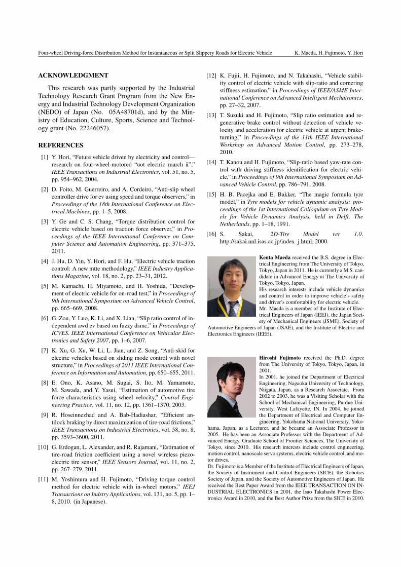
Kenta Maeda received the B.S. degree in Elec-trical Engineering from The University of Tokyo,Tokyo, Japan in 2011. He is currently a M.S. can-didate in Advanced Energy at The University ofTokyo, Tokyo, Japan.His research interests include vehicle dynamicsand control in order to improve vehicle’s safetyand driver’s comfortability for electric vehicle.Mr. Maeda is a member of the Institute of Elec-trical Engineers of Japan (IEEJ), the Japan Soci-ety of Mechanical Engineers (JSME), Society of

Automotive Engineers of Japan (JSAE), and the Institute of Electric andElectronics Engineers (IEEE).

Hiroshi Fujimoto received the Ph.D. degreefrom The University of Tokyo, Tokyo, Japan, in2001.In 2001, he joined the Department of ElectricalEngineering, Nagaoka University of Technology,Niigata, Japan, as a Research Associate. From2002 to 2003, he was a Visiting Scholar with theSchool of Mechanical Engineering, Purdue Uni-versity, West Lafayette, IN. In 2004, he joinedthe Department of Electrical and Computer En-gineering, Yokohama National University, Yoko-

hama, Japan, as a Lecturer, and he became an Associate Professor in2005. He has been an Associate Professor with the Department of Ad-vanced Energy, Graduate School of Frontier Sciences, The University ofTokyo, since 2010. His research interests include control engineering,motion control, nanoscale servo systems, electric vehicle control, and mo-tor drives.Dr. Fujimoto is a Member of the Institute of Electrical Engineers of Japan,the Society of Instrument and Control Engineers (SICE), the RoboticsSociety of Japan, and the Society of Automotive Engineers of Japan. Hereceived the Best Paper Award from the IEEE TRANSACTION ON IN-DUSTRIAL ELECTRONICS in 2001, the Isao Takahashi Power Elec-tronics Award in 2010, and the Best Author Prize from the SICE in 2010.


Yoichi Hori received the B.S., M.S., and Ph.D.degrees in electrical engineering from The Uni-versity of Tokyo, Tokyo, Japan, in 1978, 1980,and 1983, respectively.In 1983, he joined the Department of ElectricalEngineering, The University of Tokyo, as a Re-search Associate, where he later became an As-sistant Professor, an Associate Professor, and, in2000, a Professor. He moved to the Institute ofIndustrial Science as a Professor with the Infor-mation and System Division in 2002 and to the

Department of Advanced Energy, Graduate School of Frontier Sciences,The University of Tokyo, in 2008. From 1991 to 1992, he was a VisitingResearcher with the University of California, Berkeley. His research in-terests are control theory and its industrial applications to motion control,mechatronics, robotics, electric vehicles, etc.Dr. Hori has been the Treasurer of the IEEE Japan Council and TokyoSection since 2001. He is also an Administrative Committee memberof the IEEE Industrial Electronics Society and a member of the Societyof Instrument and Control Engineers, the Robotics Society of Japan, theJapan Society of Mechanical Engineers, and the Society of AutomotiveEngineers of Japan (JSAE). He was the President of the Industry Appli-cations Society of the Institute of Electrical Engineers of Japan (IEEJ),the President of Capacitors Forum, the Chairman of the Motor Technol-ogy Symposium of the Japan Management Association, and the Directoron Technological Development of JSAE. He received the Best Transac-tions Paper Award from the IEEE TRANSACTION ON INDUSTRIALELECTRONICS in 1993 and 2001, the 2000 Best Transactions PaperAward from the IEEJ, and the 2011 Achievement Award from the IEEJ.

AUTHORS’ ADDRESSESKenta MaedaProf. Hiroshi Fujimoto, Ph.D.Prof. Yoichi Hori, Ph.D.Department of Advanced Energy,Graduate School of Frontier Sciences,The University of Tokyo,5-1-5, Kashiwanoha, Kashiwa, Chiba, 277-8561, Japanemail: [email protected],[email protected], [email protected]

Documents

Four-wheel Driving-force Distribution Method for ...hflab.k.u-tokyo.ac.jp/papers/2013/maedaAUTOMATIKA13.pdf · Four-wheel Driving-force Distribution Method for Instantaneous or Split