Noname manuscript No.(will be inserted by the editor)

Four-Objective Formulations of Multicast Flows ThroughEvolutionary Routing with QoS and Traffic Engineering

Marcos L. P. Bueno · Gina M. B. Oliveira

Received: date / Accepted: date

Abstract In this work, we investigate multiobjective

formulations of multicast routing, in which a tree must

be set to deliver data to a subset of destination nodes

in a network. Two four-objective formulations are con-

sidered, for which we propose a multiobjective evolu-

tionary model, composed by the well-known SPEA2

(Strength Pareto Evolutionary Algorithm 2) scheme as

underlying search, and three heuristics (h2, h3 and h4)

incorporated into crossover and mutation operators. Over

seven instances of the problem and five metrics to assess

convergence, diversity and coverage, our designed ex-

periments showed that the combined heuristic (namely,

h4) overcame heuristics h2 and h3 on convergence, while

returning solutions that covered the objective space

as well as heuristic h2. Such analysis was reinforced

through non-parametrical statistical significance tests,

followed by a comparison of our model with well-known

Dijkstra’s and Takahashi-Matsuyama algorithms, show-

ing that our genetic model returned better solutions.

Keywords multicast routing · traffic engineering ·multiobjective optimization · genetic algorithm ·heuristics

1 Introduction

In computer networks, a routing algorithm is responsi-

ble for calculating paths in which data flows will tran-

sit between network links. In such context, the network

Marcos Luiz de Paula Bueno and Gina Maira Barbosa de Oliveira

Faculty of Computer Science - Federal University of Uberlandia

- Av. Joao Naves de Avila 2160, Bloco B. Uberlandia, MinasGerais, 38400-902, Brazil

Tel/Fax: +55 34 3239 4144

E-mail: marcos@facom.ufu.brE-mail: gina@facom.ufu.br

topology is usually modeled as a connected graph, in

which vertices represent routers, while edges represent

physical links. Depending on the purpose of the data

transmission between network nodes (hosts, routers,

etc.), several kinds of routes can be established. For

instance, unicasting corresponds to transmit data in a

point-to-point fashion, being largely used in the Inter-

net [33]. On the other hand, broadcasting is another

kind of data transmission, in which data is sent to all

destinations, used, for example, to transmit weather re-

ports, live radio programs or when routers exchange

information related to network topology in link state

protocols [21].

Many algorithms are used to compute such routes,

like Dijkstra’s and Bellman-Ford ones [10] for the uni-

cast case, and Dalal & Metcalfe’s reverse path forward-

ing [13], spanning trees and flooding mechanism [33]

for the broadcast case. In the Best Effort service es-

tablished in the Internet, these algorithms can provide

good quality of routes when only one metric is con-

sidered at any given time. More specifically, when such

metric is an end-to-end one (e.g. end-to-end delay, hops

count), algorithms like Dijkstra’s can guarantee the op-

timality of unicast routes, since the problem is the same

of calculating shortest paths in graphs.

Multicasting, in turn, is intended to send data to a

subset of hosts in the network. The main motivation to

this kind of transmission is to save network resources,

duplicating packets only when routing paths branches.

A multicast route is, then, modeled as a tree, in which

data is sent from a source node, passing by several inter-

mediary nodes to reach destination ones. In this sense,

it can be cheaper than establishing multiple unicast

transmissions to deliver data through a path to each

destination, and significant economies over unicast can

be achieved. The study of pricing policies and tariffs is

2

an important issue in this context, due to these different

features of unicast and multicast [9]

The difficulty of multicast problem is the same of

shortest path calculation when the metric to be op-

timized is an end-to-end one, like end-to-end delay or

end-to-end hops count, since the problem is, in fact, the

same of calculating optimal unicast paths. However, if

one wants to optimize some metric related to the tree,

such as its cost or its length (i.e. the number of edges),

the problem would become the well-known Steiner Tree

Problem in Graphs (STP), which is known to be in the

NP-hard class of problems, as showed by Karp [18].

Moreover, in many applications of multicasting (e.g.

multimedia ones) the route quality is related to the

achievement of multiple requirements, such as fast com-

munication with low delay, reliably and low cost. Re-

quirements like these are related to Quality of Service

(QoS) concept [30], [33], which deal with special treat-

ments required by a service to provide performance as-

surances, impacting on the user’s satisfaction.

On the other hand, Traffic Engineering (TE) is con-

cerned with improving network performance aiming to

reduce congestion bottlenecks, improve resource utiliza-

tion and also to provide adequate QoS for final users

[3]. Such aims can be achieved by establishing routes

in such a way that the traffic distribution is balanced.

When QoS and TE requirements are also being consid-

ered in multicast routing, it leads to the need of opti-

mizing a set of objectives subject to constraints. Thus,

different conflicting objectives are established and the

route calculus can be seen as a multiobjective problem

[15].

Given a weighted network and a new multicast flow

φ to be loaded on it, in the Multicast Flow Routing

Problem (MFRP) we want to calculate Pareto-optimal

trees to carry that flow over the net. Two formulations

of MFRP were considered in this work, minimizing the

following objective functions: maximum link utilization,

total cost, maximum end-to-end delay, mean end-to-end

delay and hops count, subject to a link capacity con-

straint. Since MFRP can be considered as an extension

of the Steiner Tree Problem, many techniques have been

used to tackle MFRP, such as heuristics, approximation

algorithms and related artificial intelligence techniques

[1], [4], [14], [15], [26], [32], [2], [31]. In this work, we

use multiobjective evolutionary algorithms (MOEAs)

to tackle MFRP, since they have been used in several

works ([27], [39], [12], [22], [11], [25], [24], [23], [6]) with

promising results. SPEA2 (Strength Pareto Evolution-

ary Algorithm 2) is one of the most successful MOEAs

investigated in the literature [40], [43], [42], [41].

This work evaluates three heuristics for crossover

and mutation operators incorporated along multiob-

jective evolutionary algorithms (MOEAs) designed to

solve MFRP. Such heuristics are evaluated with a SPEA2-

based environment, through experiments with seven in-

stances of MFRP and five metrics to assess convergence

and diversity. In our designed scenarios, we were able

to conclude that when combined with one of the heuris-

tics (heuristic h4), SPEA2 returned the best results on

the overall average by a significant percent, compared

to SPEA2 with the other two heuristics. A comparison

with traditional algorithms from the literature (Dijk-

stra’s and Takahashi-Matsuyama [32]) is carried out,

showing that our evolutionary environment can provide

better solutions than those algorithms in most cases.

Besides, if small levels of tolerance over delay and cost

are allowed, more expressive gains can be obtained for

the other objective functions, when compared with the

solutions provided by these algorithms.

The remainder of this paper is organized as follows:

in Section 2 a description of Multicast Routing Problem

tackled in this paper is presented; Section 3 briefly re-

lates a few related works from the literature; the un-

derlying model is presented at Section 4, while the pro-

posed heuristics are shown in Section 5; finally, the ex-

perimental results and final remarks are discussed in

sections 6 and 7.

2 Multicast Flow Routing Problem

In this work, routing with QoS and TE requirements

is considered under a multiobjective optimization view.

In that case, it may not be possible to optimize all ob-

jectives simultaneously, because when optimizing one

or more objectives, we could deteriorate another(s).

If that is the case, it may not exist a solution that

has, simultaneously, optimal values for each objective.

Due to this conflict, we use a strict partial order rela-

tion known as Pareto dominance[29]: given two n-

dimensional decision vectors a and b and their respec-

tive objective vectors f(a) = {f1(a), . . . , fm(a)} and

f(b) = {f1(b), . . . , fm(b)}, we say a dominate b (a ≺ b,

in symbols) iff:

– a is not worse than b in any objective; and

– a is strictly better than b in at least one objective.

In a Pareto dominance relation, for any two vectors

a and b, may not occur a ≺ b nor b ≺ a. Inside a set of

solutions, those for which there is no other that dom-

inates them are called nondominated solutions. Thus,

in a global sense, if P is the entire decision space, then

a feasible solution x∗ ∈ P is called Pareto-optimal so-

lution iff 6 ∃x ∈ P, x ≺ x∗. The set composed by all

Pareto-optimal solution is called global Pareto-optimal

set, denoted by P ∗.

3

Considering a multicast context, the network topol-

ogy is modeled as a connected undirected graph G =

(V,E,W ), such that V represents a set of nodes or ver-

tices, E a set of edges and W a tuple o weights. We de-

fine r ∈ V as the source or root node and a set D ⊂ Vas the multicast group, in which each node is called

destination or terminal. For each edge e in G, there is

a tuple W = (c(e), d(e), z(e), t(e)), corresponding to an

edge’s cost, delay, capacity and current traffic, respec-

tively, which are defined on R. Since each edge has a

capacity, we have the following restriction over the traf-

fic passing by it at any moment: t(e) ≤ z(e),∀e ∈ E.

Finally, there is a new traffic request φ ∈ R that we

want to load on G.

Thus, in Multiobjective Multicast Flow Routing Pro-

blem (MFRP), given an instance (G, r,D, φ), we want

to calculate trees T = (VT , ET ) of G, rooted in r, with

{r} ∪D ⊆ VT , such that T will allow the loading of φ

into G. In order to load φ into G, every feasible can-

didate T (also called multicast tree) must attend the

constraint t(e) + φ ≤ z(e),∀e ∈ ET . We also want to

minimize five objective functions for each T :

a. Cost of the tree:

cost(T ) =∑e∈ET

c(e) (1)

b. Mean end-to-end delay:

D(T ) =

∑delay(ti)

|D|(2)

c. Maximum end-to-end delay:

D(T ) = max {delay(ti)} , i = 1, . . . , |D| (3)

d. Hops count:

hops(T ) = |ET | (4)

e. Maximum link utilization (bottleneck):

α(T ) = max

{t(e) + φ

z(e)

},∀e ∈ ET (5)

We consider the following constraint:

f. Edge’s capacity:

t(e) + φ ≤ z(e) (6)

where e ∈ ET and delay(ti) =∑

e∈path(r,ti) d(e),∀ti ∈D. Thus, given the two formulations for MFRP below

(Multiobjective Optimization Problems or MOPs), we

want to calculate the Pareto-optimal set of solutions,

such that:

– P1: min α(T ), cost(T ), D(T ) and hops(T )

subject to Eq. 6.

– P2: min α(T ), cost(T ), D(T ) and D(T )

subject to Eq. 6.

An instance of MFRP is shown on Figure 1, con-

sisting on a network with 18 nodes, in which node 0 is

the source and nodes 6, 10, 13, 15, 17 are the terminal

ones. For each edge e, the weights cost, delay and cur-

rent traffic (c(e), d(e), t(e)) are explicit presented. On

the other hand, capacity z(e) is considered fixed for all

the edges (z(e) = 12 Mbps,∀e ∈ E) and it is omitted

in the figure. A Pareto-optimal solution for such G, D,

r and φ = 2.0 Mbps on P1 and P2 is showed by the

tree on right side of the figure, along with its objective

values.

Fig. 1: A MFRP instance on left (φ = 2.0), and a

Pareto-optimal solution on right, whose objectives are

α(T ) = 0.85, cost(T ) = 71 ∗ 2.0, D = 9.8, D(T ) = 12

and hops(T ) = 9.

3 Related Literature

Due to the computational complexity of routing pro-

blem, there is a large number of works focusing on its

variations. For the Unicast Routing Problem (URP)

with one objective, there are efficient algorithms for

shortest path calculation, such as Bellman-Ford’s and

Dijkstra’s [10], which are used in RIP and OSPF pro-

tocols [33]. On the other hand, URP with two or more

aditive and/or multiplicative metrics is a NP-complete

problem, as proved in [37], in which efficient algorithms

were presented for a simplified decision version for URP.

On the other hand, multicast routing and Steiner

problems (STP) have been tackled in several investi-

gation lines. Dreyfus and Wagner [14] proposed an ex-

act algorithm to solve STP with complexity O∗(3|D|),

based on dynamic programming and using a shortest

path algorithm to calculate Steiner subtrees as the main

idea. There are also several heuristics procedures for

STP. In [2] it is proposed a local optimization procedure

4

with Takahashi-Matsuyama heuristic [32]. Such heuris-

tic uses Dijkstra’s algorithm to build a solution from a

incremental union of a shortest path from each desti-

nation to the current tree – an idea similar to Prim’s

algorithm [10]. Other approaches with various kinds

of metaheuristic models, such as GRASP [31], Parti-

cle Swarm Optimization (PSO) [36], Simulated Anneal-

ing [38] and Tabu Search [16], were proposed in recent

years.

In a very useful variation of the Steiner Tree Pro-

blem (also known as Constrained STP or CSTP) in

routing applications, a heuristic is proposed in [28] con-

sidering maximum end-to-end delay and delay variation

metrics, which main idea is the creation of solutions

from K shortest paths computation. Kompella et al.

[19], in turn, proposed a dynamic programming-based

heuristic to tackle CSTP with maximum delay restric-

tion. Ravi [26] presents approximation algorithms com-

bined with local optimization for several variations of

Steiner problem.

Several works use genetic algorithm-based approaches

for variations of Multicast problem. In [27] the authors

presents a mono-objective genetic algorithm (GA) using

the objectives cost, delay and bandwidth aggregated in

a weighted expression. Such GA model was improved

in [39], adding changes in crossover and using elitism

in reinsertion. The model presented in [22] was based

on those works, fulfilling some gaps left there, like the

choice of reconnection algorithm in crossover and mu-

tation. Such work also proposed a mechanism to in-

crease population diversity called filter. The authors in

[23] proposed a model also based on the one described

in [27], but in multiobjective perspective, where they

applied several MOEAs based on the family of NSGA

(Non-dominated Sorting Genetic Algorithm) methods

- NSGA, NSGA-II and ε-NSGA-II - also evaluating a

few crossover changes.

Regarding Routing with flows, a NSGA-based [43]

MOEA with 3 objectives and 1 restriction was proposed

in [12], using an entropy mechanism to increase pop-

ulation diversity. In [11] it is proposed a SPEA-based

approach with four-objective and one constraint, devel-

oping a crossover and mutation based on pre-calculated

shortest paths, while in [25] the authors also used a

SPEA-based approach, but using 5 objective functions.

A survey in which are evaluated a large number of GAs

proposals for routing is presented in [15], where they

also propose a SPEA-based MOEA considering 11 ob-

jective functions and some statistical analysis, such as

correlation between objective functions.

4 Evolutionary Routing

4.1 Multiobjective Evolutionary Algorithms

Genetic Algorithms (GAs) are stochastic search meth-

ods for problem solving, inspired on biological evolution

theory [17]. The main metaphor with the biological the-

ory is that the more adapted individuals in their envi-

ronment tend to survive and reproduce, hoping that

their offspring should be at least adapted as their par-

ents. In this manner, from natural selection and genetic

inheritance, it is expected to occur the evolution of pop-

ulation. GAs are also included on metaheuristic meth-

ods, since they use some kind of approximated infor-

mation (the fitness value) to guide the search towards

more promising points, to achieve the optimal solution.

Multiobjective Evolutionary Algorithms (MOEAs)

are evolutionary algorithms designed to approach prob-

lems that includes more than one objective to optimize,

usually considering the Pareto dominance relation. The

main difference between a classic GA and a MOEA usu-

ally lies on fitness assignment, where dominance can be

used in different ways. This work deals with the model

SPEA2 from the second generation of MOEAs, briefly

described in the following.

Strength Pareto Evolutionary Algorithm 2 (SPEA2)

[42] is a MOEA proposed by Zitzler et al., character-

ized by maintaining, besides the current population, an

external file to keep the non-dominated solutions found

so far. The procedure to calculate fitness is based on

the ideas of dominance count and dominance rank [41],

which refer to how many individuals are dominated by

each individual, and how many individuals that dom-

inate it, respectively. Such procedure encompasses the

concept of using one population to evaluate another.

SPEA2 came to improve its predecessor SPEA [43],

mainly in three aspects. Firstly, providing a more com-

plete assignment of fitness, in which dominance infor-

mation among population members is considered, since

in SPEA the fitness of population members depends on

the strength (the number of individuals that it domi-

nate) of its dominators only, possible leading to a reduc-

tion over the selection pressure. Another difference with

SPEA is that, for each individual, a density estimation

is used to guide the search more efficiently, specially

when there are many non-dominated individuals in the

current generation, being used to differentiate between

them. Finally, another procedure (based on k-th near-

est neighbor) to reduce the cardinality of the external

archive is proposed, where extreme solutions are pre-

served.

In a previous paper [7], several experiments were

performed and it was possible to verify that SPEA2

5

overcame SPEA in MFRP, through several metrics on

various instances. The present work focus on a compre-

hensive evaluation of crossover heuristics through punc-

tual estimations and statistical significance tests, and

showing a comparison with traditional algorithms used

in Routing and Steiner’s literature, as shown in Section

6.

4.2 The Proposed Model

In the following, we describe the major aspects of the

evolutionary models implemented in the present work

to solve MFRP. These steps were based on the original

mono-objective model proposed in [27] and refined in

the subsequent mono-objective models in [39] and [22].

The major steps of the model described in [27] were

also used in the multiobjective models proposed in [25]

and [23], where [23] uses NSGA-II and [25] uses SPEA

as underlying multiobjective approaches. The remain-

ing steps omitted here are discussed in these previous

works, specially in reference [23].

4.2.1 Initial population

Each individual is codified directly as a generic rooted

tree, as exemplified in right side of Figure 1. Each tree

is generated by a random search algorithm, in which

nodes are randomly inserted in the tree until all desti-

nation nodes are inserted. Then, a pruning is applied

over the tree, so that every leaf node will be a destina-

tion one. Note that this algorithm has the same worse

case complexity of breadth-first or depth-first search,

i.e., O(|E| + |V |) since the only difference is that we

choose the next neighbor to expand in a random way,

instead of using a queue or a stack.

4.2.2 Crossover

The crossover operator presented here is based on the

general scheme proposed in [27] and [23]. From two par-

ents, a child inherit their features following these gen-

eral steps:

(i) identification of common edges between two par-

ents, resulting in a forest of subtrees;

(ii) random choice of a weight of G (cost, delay or

current traffic) to be used along reconnections;

(iii) reconnection of subtrees, resulting on a new mul-

ticast tree containing all destination nodes; and

(iv) pruning of useless nodes, i.e., a recursive proce-

dure that remove terminal nodes of the tree that

are not destination ones.

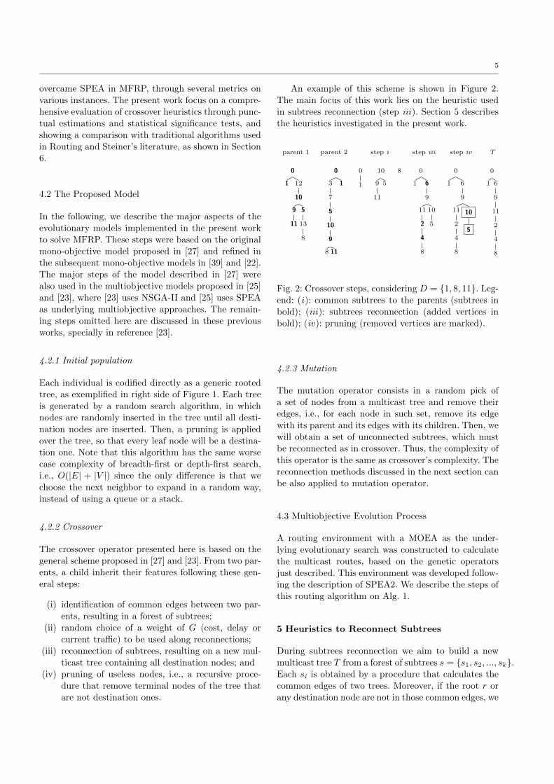
An example of this scheme is shown in Figure 2.

The main focus of this work lies on the heuristic used

in subtrees reconnection (step iii). Section 5 describes

the heuristics investigated in the present work.

parent 1 parent 2 step i step iii step iv T

0

1 12

10

9

11

5

13

8

0

3

7

5

10

9

8 11

1

0

1

10

9

11

5

8 0

1 6

9

11

2

4

8

10

5

0

1 6

9

11

2

4

8

10

5

0

1 6

9

11

2

4

8

Fig. 2: Crossover steps, considering D = {1, 8, 11}. Leg-

end: (i): common subtrees to the parents (subtrees in

bold); (iii): subtrees reconnection (added vertices in

bold); (iv): pruning (removed vertices are marked).

4.2.3 Mutation

The mutation operator consists in a random pick of

a set of nodes from a multicast tree and remove their

edges, i.e., for each node in such set, remove its edge

with its parent and its edges with its children. Then, we

will obtain a set of unconnected subtrees, which must

be reconnected as in crossover. Thus, the complexity of

this operator is the same as crossover’s complexity. The

reconnection methods discussed in the next section can

be also applied to mutation operator.

4.3 Multiobjective Evolution Process

A routing environment with a MOEA as the under-

lying evolutionary search was constructed to calculate

the multicast routes, based on the genetic operators

just described. This environment was developed follow-

ing the description of SPEA2. We describe the steps of

this routing algorithm on Alg. 1.

5 Heuristics to Reconnect Subtrees

During subtrees reconnection we aim to build a new

multicast tree T from a forest of subtrees s = {s1, s2, ..., sk}.Each si is obtained by a procedure that calculates the

common edges of two trees. Moreover, if the root r or

any destination node are not in those common edges, we

6

Algorithm 1 SPEA2-based routing algorithm

Input: Npop: number of multicast trees in population P ;

Nger: number of generations; L: maximum size of E.Output: E: a set of non-dominated multicast trees found

during the search.

1: Generate an initial population P0 with Npop random multi-

cast trees

2: E0 ← ∅3: t← 0

4: while true do

5: Calculate fitness for each tree of Pt ∪Et, according to theformulation (P1 or P2)

6: Assign Et+1 with non-dominated trees from Pt ∪ Et

7: if |Et+1| < L then Fill Et+1 with the fittest dominatedtrees from P

8: else if |Et+1| > L then Apply truncation procedure toreduce Et+1 size

9: if t > Nger then

10: Return non-dominated trees from Et+1 (end of exe-

cution)

11: Select Npop pairs of trees (parents) from Et+1 using afitness-based binary tournament

12: Apply crossover and mutation over the parents to gener-

ate Pt+1

13: t← t+ 1

build and add isolated subtrees, i.e., subtrees that con-

tains only one vertex, into s. We start the reconnections

randomly selecting subtrees si and sj and calculate a

set p of edges such that si ∪ p ∪ sj will be a connected

subgraph of G. In the following reconnections, we se-

lect another subtree and calculate a new set p between

it and the subgraph obtained on the previous reconnec-

tion. Therefore, |s|−1 reconnections will be made until

all subtrees are reconnected to produce a new tree with

all destination nodes.

An important decision that affects the convergence

of GA to optimal solutions is how to choose the edges

of p; this aspect is explored by the heuristics described

next. Heuristics h2 and h3 were also presented in a sim-

plified form on references [6], [7]. Heuristic h2 have an

O(|V |2) worse case complexity, while h3 and h4 have

an O(|V ||E| log |V |) complexity.

5.1 Heuristic h2

Heuristic h2 is based on the original heuristic proposed

by Ravikumar & Bajpai [27], but includes some im-

provements to avoid the potential occurrence of loops.

It uses a shortest path algorithm to select a set p of

edges at each reconnection. Here we employed the same

shortest path method used in [22] and [23]: Dijkstra’s

algorithm. The use of such algorithm is an attempt to

improve the fitness of each individual, being interesting

under runtime perspective, since it has O(|E| log |V |)

time complexity if a binary heap is used [10]. Lines 1

and 3-12 on Alg. 2 defines h2.

In Algorithm 2, the general idea is that, after initial-

izing T , the reconnection loop builds T from successive

reconnections with others si by calculating a shortest

path p. In other words, we randomly pick the next si,

and calculate the shortest path p between it and T . A

procedure to rotate si is called to change its root, en-

suring that the root of s‘i will be the last vertex of p.

However, each time a shortest path p is calculated, it is

possible that it include vertices from one or more sub-

trees of s not yet reconnected. Thus, since we will have

to join those remaining subtrees from s in a posterior

reconnection, loops would be formed in T .

The test to check whether would occur a conflict

when joining T and s‘i consists in checking if p has only

one edge with the same ends. If there is a conflict, h2

strategy determines to insert only edges (x, y) from s‘isuch that the vertex y does not exist in T . That is

because, if we allow such insertion, the vertex y would

be repeated in tree T , what would turn the solution an

invalid one. On the other hand, if there is no conflict, we

unite T with p and s‘i. This whole reconnection process

is done until there are no more subtrees to reconnect

with T .

5.2 Heuristic h3

Differently from the previous method, in h3 the parent

similarity information is never lost when reconnecting

subtrees. The shortest path calculation is not used by

h3, in which the path p is randomly calculated. Lines 1

and 14 to 21 of Alg. 2 formalize this process.

The heuristic h3 starts with T corresponding to the

subtree which contains root node. Then, T is randomly

filled in with the same idea of random search algorithm

used in initial population generation, until appears a

node existing in any subtree si not yet reconnected. At

this moment, we rotate si and unite it with T . The algo-

rithm repeats these operations while there is a subtree

to reconnect.

5.3 Heuristic h4

In previous papers [6], [8], [5], [7], experiments con-

ducted over some instances of MFRP indicated that

h2 returned a better GA convergence. However, in an-

other instances, such behavior was accomplished with

heuristic h3. Thus, heuristic h4 proposes a combination

of heuristics in the following way: at the beginning of a

crossover, after calculation of common subtrees and the

choice of weight of edge, we randomly choose which of

7

the two heuristics will be used to perform reconnections

of subtrees forest s. Thus, h4 is simply a random choice

between h2 and h3 at the beginning of each crossover.

The entire Alg. 2 describes the heuristic h4. Notice that,

using heuristic h4 the validity of final T is preserved, be-

cause on this scheme each crossover can be done using

h2 or h3, which generates only valid trees as discussed

previously.

Algorithm 2 Heuristic h4 to reconnect subtrees

Input: G = (V,E): connected graph; s: set of subtrees.Output: T = (VT , ET ): a multicast tree rooted in r, such

that D ⊂ VT .

1: T ← s02: if rand = 0 then . will execute h2

3: while there is a subtree to reconnect do4: Randomly pick the next subtree si5: p← shortestPath (T, si)

6: s‘i ← rotate (si, p.end)7: if there is conflict on p then

8: for each edge (x, y) ∈ s‘i do

9: if y /∈ VT then T ← T ∪ {(x, y)}10: else11: T ← T ∪ p12: T ← T ∪ s‘i13: else . will execute h314: while there is a subtree to reconnect do

15: u← pickParent (T )

16: v ← pickChild (G,T, u)17: T ← T ∪ {(u, v)}18: if v exists in any si not reconnected yet then

19: s‘i ← rotate (si, v)20: T ← T ∪ s‘i21: return T

6 Experimental Results

The performance of reconnection heuristics (h2, h3 and

h4) was experimentally evaluated on each of the two

formulations of PFRM over seven instances taken from

Routing and Steiner’s literature [39],[27], [35], [6], pre-

sented in Tab. 1. This table also shows the cardinality

of each reference set P ∗ for each instance. The original

definition of edge’s weights of nets 0, 1 and 2 had val-

ues for cost and delay, while nets 3 to 6 had only values

of cost. Thus, we generated random values for delay

to nets 3 to 6, uniformly distributed over the interval

[1, 15]. Since the weights related to capacity and current

traffic are also needed, random values for that weights

were generated over the interval [1000, 1500] Kbps and

[0, 500] Kbps, respectively, (nets 0 to 6).

The GA parameters - size of population (Npop) and

number of generations (Nger) - were set as: Npop = 30

Table 1: Summary of instances and their cardinalities

of Pareto-optimal sets for each formulation.

Instance |V | |E| |D| |P1∗| |P2∗|0 15 44 5 27 28

1 18 50 5 7 122 33 106 10 122 180

3 50 126 12 40 91

4 75 188 19 72 1285 75 188 38 60 76

6 75 300 13 42 151

and Nger = 50 for networks 0 and 1, and Npop = 90

and Nger = 100 for networks 2 to 7. The probability

of mutation occurrence is 10%, and node disconnection

rate in mutation is 20%

6.1 Metrics to Assess Convergence and Diversity

Regarding the design of experiments to evaluate models

in problems with multiple objectives, two main goals in

multiobjective optimization must be considered: con-

vergence and diversity. The first one assess the quality

of the approximation of a set of solutions P returned

by an algorithm to a reference Pareto-optimal set P ∗.

On the other hand, solutions of P should be well spread

along the objective space, leading us to metrics like cov-

erage of the objective space (e.g. in terms of extreme

solutions). Therefore, many metrics were described in

the literature to evaluate different aspects of these two

goals, in order to provide a set of values that can be

used in the decision making process.

In this work, the following metrics were considered

to assess convergence:

– Error Rate (er): corresponds to the percent of so-

lutions of P that are not Pareto-optimal ones [34].

In symbols:

er =

|P |∑i=1

ei

|P |where ei = 1 if solution i ∈ P is dominated by

any solution of P ∗; otherwise, ei = 0. The bigger

the value of er, the worst will be relative conver-

gence, i.e., the percent of solutions of P that are

not Pareto-optimal solutions. Therefore, this metric

must be minimized.

– Generational Distance (gd): corresponds to the

mean distance between the vectors of P and P ∗ [34].

In symbols:

gd =

√√√√ |P |∑i=1

d2i

|P |

8

where di = minj∈P∗

d(i, j), i.e., for each vector i ∈ P , we

find its nearest vector j ∈ P ∗ in terms of Euclidian

distance. The smaller the value of gd, more closer

to P ∗ will be the set P . Thus, this metric must be

minimized.

– Pareto Subset (ps): corresponds to the absolute

number of solutions of P that are Pareto-optimal

ones:

ps = (1− er)|P |

This metric complement the information given by

er, however in a contrary direction (i.e. the number

of solutions that are Pareto-optimal, instead of the

percent of solutions that are not Pareto-optimal) in

an absolute sense. This metric must be maximized.

Aiming to evaluate the distribution of solutions, the

following metric was considered:

– Maximum Spread (m3): correspond to the sume

of maximum extension obtained on each objective

by a set P [40]. Formally,

m3 =

√√√√ M∑i=1

(max fi −min fi)2

Finally, to directly compare in terms of dominance

two sets of solutions P and Q, we used the metric cov-

erage [40]:

– Two Set Coverage (sc):

sc(P,Q) =|{j ∈ Q;∃i ∈ P : i ≺ j}|

|Q|

The sc metric is not symmetric for two sets P and

Q, therefore, it is necessary to calculate sc(P,Q) and

sc(Q,P ). A value of sc(P,Q) = 1 indicates that all

solutions of Q are dominated by at least one solution of

P , while sc(P,Q) = 0 would indicate that no solution

from Q would be dominated by any solution from P .

6.2 Results on Formulations P1 and P2

The results are shown in tables 2 and 3, in which the

higher level of gray background indicates the best re-

sults on each scenario, while the second level of gray in-

dicates the second best result; the worst result is shown

by a white background. These results are also shown in

a graphical way by figures 3, 4, 5 and 6.

The results on metric er show that nets 0 and 1

seems to be easy instances of MFRP, since all heuris-

tics reached values near to 0, specially h3 and h4. Over

the larger instances (nets 2 to 6), h4 reached the best

results on most cases. Looking at each scenario, h4 re-

turned values for er smaller than 20% in all cases (ex-

cept on net 6/P2) , while the other heuristics reached

values larger than it in some scenarios (reaching values

greater than 40% in some cases), showing less varia-

tion of the means among instances. An observation of

the general means shows that among the solutions re-

turned by h4 on P1 approximately 93% were, in fact,

Pareto-optimal ones, while such percent was 85% and

88% for h2 and h3, respectively. Regarding P2 formu-

lation, h4 also reached the best results on this metric,

returning 85% of solutions that were Pareto-optimal

ones, against 76% and 78% by h2 and h3, respectively.

In other words, the relative convergence (i.e. in terms

of percents) obtained by h4 was better than the ones

from h2 and h3.

Reinforcing these results with the metric ps, h4 also

concentrated the best results, as we can seen by the gray

levels, returning more Pareto-optimal solutions than h2

and h3. The averages indicate that h4 improved 22%

and 27% of the results on P1 obtained by h2 and h3,

respectively. Such gains over h2 and h3 were around

27% in P2. These gains were even more greater in the

larger instances (nets 2 to 6), reaching more than 50%

in some cases (e.g. nets 4 and 6 compared to h3/P1).

Analyzing the last metric for convergence (gd), we

note that since gd = 0 was not obtained by any of the

heuristics, then a value closer to zero indicates that the

dominated solutions of a set P were closer to P ∗ in the

objective space. Thus, observing the results, the solu-

tions returned by h4 were closer to the Pareto-optimal

fronts on almost all instances. The heuristic h2 reached

the worst results on most cases.

The results on m3 diversity metric show that heuris-

tics h2 and h4 achieved the best results on all cases.

However, it is not much clear the difference related to

which is the better, since there is some alternation of

the best result on each instance, although h2 reached

a little higher mean than h4 (7.87 against 7.81 on P1,

respectively). Hypothesis tests will be carried to verify

such differences.

6.3 Statistical Analysis

The previous results were shown through descriptive

statistics, more specifically by means. Since GAs are

stochastic methods and each execution works with ran-

dom samples of solutions from the search space, it is

interesting to use some statistical inference to infer pa-

rameters for a given population using such samples. In

this manner, we are able to infer if the observed dif-

ferences between the heuristics can be considered sig-

nificant or not, for a certain level of confidence α. To

9

Metric Heuristic Instance Mean

0 1 2 3 4 5 6

Error Rate

2 1.22% 4.76% 21.16% 24.00% 7.11% 10.22% 44.65% 16.16%

3 0.51% 0.48% 11.58% 6.69% 14.84% 3.78% 44.59% 11.78%

4 0.65% 1.90% 10.42% 5.27% 7.16% 0.63% 20.63% 6.67%

Pareto Subset

2 21.37 6.37 63.00 25.00 46.37 43.97 19.53 32.23

3 25.60 6.97 68.30 28.07 31.80 45.93 10.60 31.04

4 25.10 6.87 80.47 32.70 50.57 55.07 24.30 39.30

Generational

Distance

2 1.23 9.90 2.08 4.58 0.67 1.22 6.27 3.71

3 0.72 1.23 1.70 1.32 1.69 0.17 5.42 1.75

4 0.46 4.90 1.30 0.45 0.57 0.10 3.74 1.65

Maximum

Spread

2 8.08 8.43 8.64 7.47 8.11 5.33 9.03 7.87

3 8.05 7.97 8.24 7.06 7.69 3.55 5.07 6.81

4 8.08 8.05 8.79 7.34 8.17 5.31 8.92 7.81

Table 2: Values for convergence and diversity metrics on formulation P1. The best results are shown by bold face.

Metric Heuristic Instance Mean

0 1 2 3 4 5 6

Error Rate

2 14.45% 1.57% 28.21% 22.66% 13.79% 31.54% 52.06% 23.47%

3 2.05% 0.00% 18.01% 3.78% 36.16% 28.31% 63.50% 21.69%

4 3.06% 0.00% 17.44% 4.91% 17.18% 16.40% 44.43% 14.78%

Pareto

Subset

2 18.47 8.57 64.27 48.07 49.90 26.20 38.43 36.27

3 25.87 11.43 71.80 61.60 28.20 35.17 18.83 36.13

4 24.50 11.07 74.30 70.17 53.77 44.83 43.63 46.04

Generational

Distance

2 9.60 3.97 2.09 2.45 2.60 1.04 2.86 3.52

3 1.29 0.00 1.54 0.78 4.57 2.92 3.90 2.14

4 2.07 0.00 1.40 0.61 2.37 0.47 2.20 1.30

Maximum

Spread

2 9.36 9.28 9.58 9.03 10.90 6.77 11.28 9.46

3 8.86 9.18 8.84 8.13 9.87 3.24 6.36 7.78

4 8.87 9.18 9.88 9.02 10.98 6.77 11.13 9.41

Table 3: Values for convergence and diversity metrics on formulation P2. The best results are shown by bold face.

accomplish that, we choose the Wilcoxon Signed-Rank

Test [20], a non-parametric hypothesis testing proce-

dure. Such test is a distribution-free one, which means

that it is not necessary that the original probability

distribution must be Normal.

The following hypothesis were formulated, consid-

ering a two-tailed test with α = 10% (5% for each tail):

– H0: µh4 = µhx

– H1: µh4 6= µhx

where µ corresponds to the population value for a given

metric (e.g. er), while hx corresponds to heuristics h2

or h3.

As usual, for such Wilcoxon test, we calculate w =

min(w+, w−), where w+ and w− are the sums of pos-

itive and negative ranks, respectively. Since the size of

our sample is 30, then we can approximate the distribu-

tion of w by a Normal one, with mean µw = n(n+ 1)/4

and variance σ2w = n(n + 1)(2n + 1)/24. Thus, we cal-

culate the test statistic z0 = (w − µw)/σw and verify

if z0 belongs to the critical region, based on reference

10

0,00%

5,00%

10,00%

15,00%

20,00%

25,00%

30,00%

35,00%

40,00%

45,00%

0 1 2 3 4 5 6

Instance

Error Rate (P1)

h2

h3

h4

(a) P1

0,00%

10,00%

20,00%

30,00%

40,00%

50,00%

60,00%

70,00%

0 1 2 3 4 5 6

Instance

Error Rate (P2)

h2

h3

h4

(b) P2

Fig. 3: Charts to represent values for Error Rate over each instance.

0,00

10,00

20,00

30,00

40,00

50,00

60,00

70,00

80,00

90,00

0 1 2 3 4 5 6

Instance

Pareto Subset (P1)

h2

h3

h4

(a) P1

0,00

10,00

20,00

30,00

40,00

50,00

60,00

70,00

80,00

0 1 2 3 4 5 6

Instance

Pareto Subset (P2)

h2

h3

h4

(b) P2

Fig. 4: Charts to represent values for Pareto Subset over each instance.

scores for a Normal distribution. If z0 does not belong

to the critical region, we accept the null hypothesis. On

the other hand, when z0 belongs to the critical region

and, therefore, the alternative hypothesis is accepted,

we will infer µh4 < µhx if w ← w+, or µh4 > µhx if

w ← w−.

For the metrics to be minimized (er and gd), when

the alternative hypothesis is accepted, the interpreta-

tion of results is as follows:

– µh4 < µhx: h4 was significantly better than hx.

– µh4 > µhx: h4 was significantly worse than hx.

When the metric is to be maximized (ps andm3) the

logic of these signals is inverted. The results of tests are

shown in tables 4 (convergence metrics) and 5 (diversity

metric). Each column has a label, representing which

test was done, i.e., h4 × h2 or h4 × h3.

The tests to compare h4 with h2 on er confirm that

h4 improved the results of h2 on er in most cases by a

significant percent. Considering both formulations, h4

achieved improved results on 9 of 14 scenarios, while h2

achieved better results only in 1 case. In the remaining

cases, no significant difference could be observed. The

heuristic h4 also returned better results than h3, how-

ever is less cases than the comparison with h2. More

specifically, h4 improved 7 of 14 scenarios, while h3 won

only in 1 scenario. In both cases, the improvements of

h4 were more noticeable on the larger instances, reflect-

ing its ability to better explore larger searches spaces.

Analogous results were obtained on tests for ps metric:

11

0,00

1,00

2,00

3,00

4,00

5,00

6,00

7,00

8,00

9,00

10,00

0 1 2 3 4 5 6

Instance

Generational Distance (P1)

h2

h3

h4

(a) P1

0,00

2,00

4,00

6,00

8,00

10,00

12,00

0 1 2 3 4 5 6

Instance

Generational Distance (P2)

h2

h3

h4

(b) P2

Fig. 5: Charts to represent values for Generational Distance over each instance.

0,00

1,00

2,00

3,00

4,00

5,00

6,00

7,00

8,00

9,00

10,00

0 1 2 3 4 5 6

Instance

Maximum Spread (P1)

h2

h3

h4

(a) P1

0,00

2,00

4,00

6,00

8,00

10,00

12,00

0 1 2 3 4 5 6

Instance

Maximum Spread (P2)

h2

h3

h4

(b) P2

Fig. 6: Charts to represent values for Maximum Spread over each instance.

h4 won h2 and h3 by 14 of 14 cases and 11 of 14 cases,

respectively.

Regarding the metric gd, h4 also returned better es-

timations in most cases, more specifically in 12 of 14 and

7 of 14 cases when compared to h2 and h3, respectively.

No improvements obtained by h2 or h3 were significant,

i.e., the remaining cases indicated that the differences

observed in samples were not statistically significant.

On the other hand, analyzing the tests on diver-

sity metric m3, h3 is clearly worse than h4. However,

there is a tight dispute between h4 and h2, in which

h2 reached slightly better results (by only 1 scenario on

each formulation).

6.4 Coverage

Our final comparison between the three heuristics is to

compare their outcomes in terms of relative dominance,

i.e., how much a non-dominated set A dominates an-

other non-dominated set B. For this, we use the two

set coverage (sc) metric explained at the beginning of

this section.

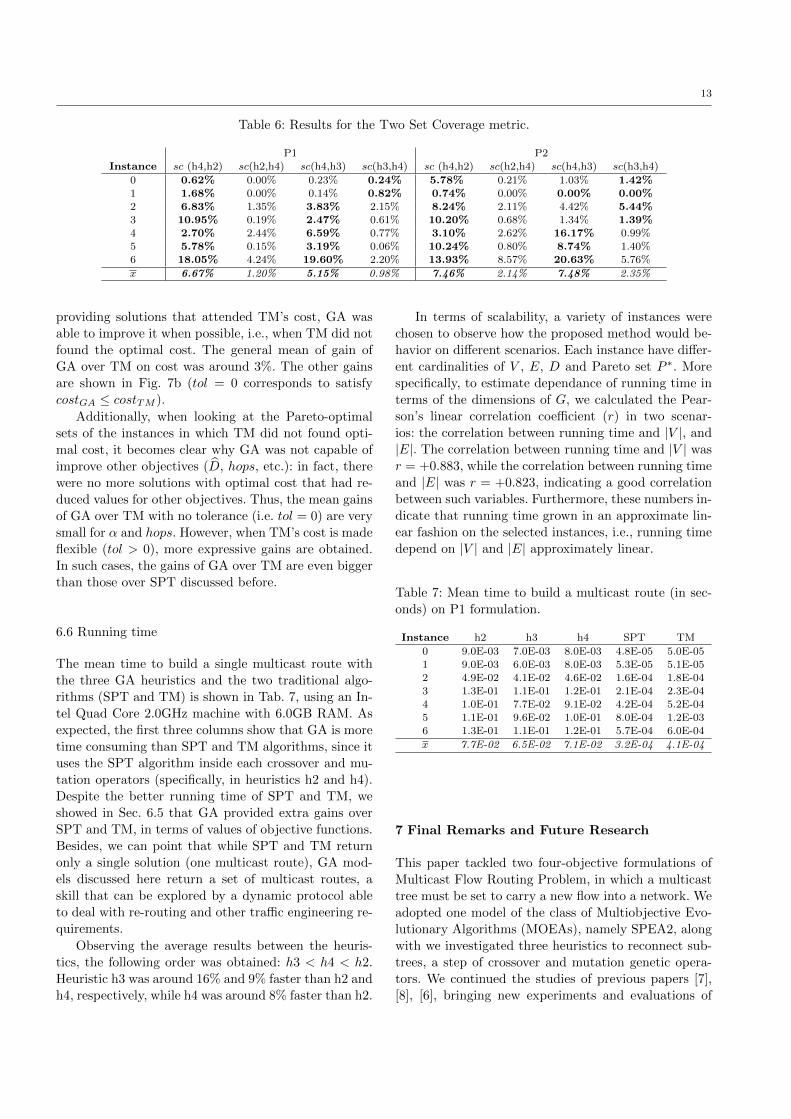
The results are shown in Tab. 6. One can observe

that the percents of domination by the solutions of h4

over h2 and h3 are much larger than the domination

of h2 and h3 over h4. These experiments reinforce that

the quality of solutions by h4 are, in general, superior

to the ones by h2 and h3.

12

P1 P2

Instance h2 h3 h2 h3

0 = = < =

1 = = = =2 < = < =

3 < < < >

4 = < > <5 < < < <

6 < < < <

(a) Error Rate

P1 P2

Instance h2 h3 h2 h3

0 > < > <

1 > = > <2 > > > >

3 > > > >

4 > > > >5 > > > >

6 > > > >

(b) Pareto Subset

P1 P2

Instance h2 h3 h2 h3

0 < = < =

1 < = < =2 < < < =

3 < < < =

4 = < = <5 < = < <

6 < < < <

(c) Generational Distance

Table 4: Results for Wilcoxon Signed-Rank hypothesis test on convergence metrics.

Table 5: Results for Wilcoxon Signed-Rank hypothesis

test on diversity metric (Maximum Spread).

P1 P2

Instance h2 h3 h2 h3

0 = = < <

1 = = = =2 > > > >

3 < > = >

4 = > = >5 < > = >

6 = > < >

6.5 Comparison with Traditional Algorithms

In this section we proceed to another kind of experi-

ment, in which the best model obtained before (SPEA2+h4)

is compared to two well-known algorithms from Rout-

ing and Steiner’s literature: Dijkstra’s algorithm (also

known as Shortest Path Tree or SPT) [10] and Taka-

hashi & Matsuyama heuristic [32].

For the comparison with SPT, we execute it to min-

imize end-to-end delay, on each instance. The main fea-

ture of SPT algorithm that is relevant in this context is

that it can guarantee the optimal end-to-end delay path

between two arbitrary vertices in a connected graph. In

this manner, GA was set to minimize the objective D

with cost, hops and α, to evidence if:

(i) in how many executions GA returned solutions with

D that attended the optimal delay given by SPT

(i.e. D = dsptmax);

(ii) when attended, which would be the gains obtained

by GA on the other objectives; and

(iii) if we define a tolerance for dsptmax, we verify if would

be any increase of the gains observed in the previous

item.

Also, one can note that in the comparison between

GA and SPT it is not possible to improve the objectiveD, since it corresponds to the average of end-to-end

delays, for which SPT gives the optimal solution, as

discussed.

The following figure of comparison was defined to

determine the gains/losses of GA over the two algo-

rithms:

g =fXi − fGA

i

fGAi

where fXi and fGAi correspond to the values of objective

i obtained by algorithm X (SPT or TM) and GA for

a given solution, respectively. Thus, when g > 0, this

metric give much a solution by X is worse compared

to the one by GA; when g < 0, the solution by GA is

worse than the one from X.

The results of the comparison with SPT indicated

that, regarding (i), GA was able to calculate solutions

that attended dsptmax on all instances. In other words, GA

achieved the same ability of SPT on calculating optimal

end-to-end delays in 100% of runs. Besides that, we also

verified that GA was able to provide other solutions

with better values for another objectives (cost, hops

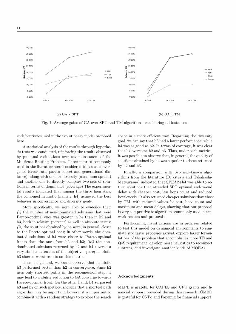
and α), as investigated by itens (ii) and (iii). These

gains, considering the general means for all instances,

are shown in Fig. 7a (tol = 0 corresponds to attend

the strict dsptmax), along with the gains obtained when

tolerances of 10% and 15% are allowed. This chart in-

dicates that GA was around 19%, 11% and 3% better

than SPT in respect of cost, hops and α, respectively.

Next, we proceed to a comparison with Takahashi

& Matsuyama heuristic [32], which provides a 2opt ap-

proximation ratio when applied to calculate the cost of

a multicast tree. We want to verify the capability of GA

to return solutions that attend or reduce the cost of so-

lutions by TM heuristic, i.e., verify if costGA ≤ costTM ,

and which would be the gains obtained in the other ob-

jectives when such condition is satisfied. The analysis

of tolerance are made as well.

Based on the gathered results, TM achieved opti-

mal cost on the smaller networks (nets 0 and 1), how-

ever, did not reached it on half of the larger nets. On

the other hand, GA was able to achieve solutions with

optimal cost on all instances. In other words, besides

13

Table 6: Results for the Two Set Coverage metric.

P1 P2Instance sc (h4,h2) sc(h2,h4) sc(h4,h3) sc(h3,h4) sc (h4,h2) sc(h2,h4) sc(h4,h3) sc(h3,h4)

0 0.62% 0.00% 0.23% 0.24% 5.78% 0.21% 1.03% 1.42%

1 1.68% 0.00% 0.14% 0.82% 0.74% 0.00% 0.00% 0.00%

2 6.83% 1.35% 3.83% 2.15% 8.24% 2.11% 4.42% 5.44%3 10.95% 0.19% 2.47% 0.61% 10.20% 0.68% 1.34% 1.39%

4 2.70% 2.44% 6.59% 0.77% 3.10% 2.62% 16.17% 0.99%

5 5.78% 0.15% 3.19% 0.06% 10.24% 0.80% 8.74% 1.40%6 18.05% 4.24% 19.60% 2.20% 13.93% 8.57% 20.63% 5.76%

x 6.67% 1.20% 5.15% 0.98% 7.46% 2.14% 7.48% 2.35%

providing solutions that attended TM’s cost, GA was

able to improve it when possible, i.e., when TM did not

found the optimal cost. The general mean of gain of

GA over TM on cost was around 3%. The other gains

are shown in Fig. 7b (tol = 0 corresponds to satisfy

costGA ≤ costTM ).

Additionally, when looking at the Pareto-optimal

sets of the instances in which TM did not found opti-

mal cost, it becomes clear why GA was not capable of

improve other objectives (D, hops, etc.): in fact, there

were no more solutions with optimal cost that had re-

duced values for other objectives. Thus, the mean gains

of GA over TM with no tolerance (i.e. tol = 0) are very

small for α and hops. However, when TM’s cost is made

flexible (tol > 0), more expressive gains are obtained.

In such cases, the gains of GA over TM are even bigger

than those over SPT discussed before.

6.6 Running time

The mean time to build a single multicast route with

the three GA heuristics and the two traditional algo-

rithms (SPT and TM) is shown in Tab. 7, using an In-

tel Quad Core 2.0GHz machine with 6.0GB RAM. As

expected, the first three columns show that GA is more

time consuming than SPT and TM algorithms, since it

uses the SPT algorithm inside each crossover and mu-

tation operators (specifically, in heuristics h2 and h4).

Despite the better running time of SPT and TM, we

showed in Sec. 6.5 that GA provided extra gains over

SPT and TM, in terms of values of objective functions.

Besides, we can point that while SPT and TM return

only a single solution (one multicast route), GA mod-

els discussed here return a set of multicast routes, a

skill that can be explored by a dynamic protocol able

to deal with re-routing and other traffic engineering re-

quirements.

Observing the average results between the heuris-

tics, the following order was obtained: h3 < h4 < h2.

Heuristic h3 was around 16% and 9% faster than h2 and

h4, respectively, while h4 was around 8% faster than h2.

In terms of scalability, a variety of instances were

chosen to observe how the proposed method would be-

havior on different scenarios. Each instance have differ-

ent cardinalities of V , E, D and Pareto set P ∗. More

specifically, to estimate dependance of running time in

terms of the dimensions of G, we calculated the Pear-

son’s linear correlation coefficient (r) in two scenar-

ios: the correlation between running time and |V |, and

|E|. The correlation between running time and |V | was

r = +0.883, while the correlation between running time

and |E| was r = +0.823, indicating a good correlation

between such variables. Furthermore, these numbers in-

dicate that running time grown in an approximate lin-

ear fashion on the selected instances, i.e., running time

depend on |V | and |E| approximately linear.

Table 7: Mean time to build a multicast route (in sec-

onds) on P1 formulation.

Instance h2 h3 h4 SPT TM

0 9.0E-03 7.0E-03 8.0E-03 4.8E-05 5.0E-05

1 9.0E-03 6.0E-03 8.0E-03 5.3E-05 5.1E-05

2 4.9E-02 4.1E-02 4.6E-02 1.6E-04 1.8E-043 1.3E-01 1.1E-01 1.2E-01 2.1E-04 2.3E-04

4 1.0E-01 7.7E-02 9.1E-02 4.2E-04 5.2E-045 1.1E-01 9.6E-02 1.0E-01 8.0E-04 1.2E-03

6 1.3E-01 1.1E-01 1.2E-01 5.7E-04 6.0E-04

x 7.7E-02 6.5E-02 7.1E-02 3.2E-04 4.1E-04

7 Final Remarks and Future Research

This paper tackled two four-objective formulations of

Multicast Flow Routing Problem, in which a multicast

tree must be set to carry a new flow into a network. We

adopted one model of the class of Multiobjective Evo-

lutionary Algorithms (MOEAs), namely SPEA2, along

with we investigated three heuristics to reconnect sub-

trees, a step of crossover and mutation genetic opera-

tors. We continued the studies of previous papers [7],

[8], [6], bringing new experiments and evaluations of

14

0,00%

5,00%

10,00%

15,00%

20,00%

25,00%

30,00%

35,00%

40,00%

tol = 0 tol = 10% tol = 15%

Gai

n o

ver

SPT

cost

hops

alpha

(a) GA × SPT

0,00%

5,00%

10,00%

15,00%

20,00%

25,00%

30,00%

35,00%

40,00%

tol = 0 tol = 10% tol = 15%

Gai

n o

ver

TM hops

alpha

Dmax

Dmean

(b) GA × TM

Fig. 7: Average gains of GA over SPT and TM algorithms, considering all instances.

such heuristics used in the evolutionary model proposed

here .

A statistical analysis of the results through hypothe-

sis tests was conducted, reinforcing the results observed

by punctual estimations over seven instances of the

Multicast Routing Problem. Three metrics commonly

used in the literature were considered to assess conver-

gence (error rate, pareto subset and generational dis-

tance), along with one for diversity (maximum spread)

and another one to directly compare two sets of solu-

tions in terms of dominance (coverage) The experimen-

tal results indicated that among the three heuristics,

the combined heuristic (namely, h4) achieved the best

behavior in convergence and diversity goals.

More specifically, we were able to evidence that:

(i) the number of non-dominated solutions that were

Pareto-optimal ones was greater in h4 than in h2 and

h3, both in relative (percent) as well in absolute terms;

(ii) the solutions obtained by h4 were, in general, closer

to the Pareto-optimal ones; in other words, the dom-

inated solutions of h4 were closer to Pareto-optimal

fronts than the ones from h2 and h3; (iii) the non-

dominated solutions returned by h2 and h4 covered a

very similar extension of the objective space; heuristic

h3 showed worst results on this metric.

Thus, in general, we could observe that heuristic

h3 performed better than h2 in convergence. Since h2

uses only shortest paths in the reconnection step, it

may lead to a ability reduction to GA converge towards

Pareto-optimal front. On the other hand, h4 surpassed

h3 and h2 on such metrics, showing that a shortest path

algorithm may be important, however it is important to

combine it with a random strategy to explore the search

space in a more efficient way. Regarding the diversity

goal, we can say that h3 had a lower performance, while

h4 was as good as h2. In terms of coverage, it was clear

that h4 overcame h2 and h3. Thus, under such metrics,

it was possible to observe that, in general, the quality of

solutions obtained by h4 was superior to those returned

by h2 and h3.

Finally, a comparison with two well-known algo-

rithms from the literature (Dijkstra’s and Takahashi-

Matsuyama) indicated that SPEA2+h4 was able to re-

turn solutions that attended SPT optimal end-to-end

delay with cheaper cost, less hops count and reduced

bottlenecks. It also returned cheaper solutions than those

by TM, with reduced values for cost, hops count and

maximum and mean delays, showing that our proposal

is very competitive to algorithms commonly used in net-

work routers and protocols.

Forthcoming investigations are in progress related

to test this model on dynamical environments to sim-

ulate stochastic processes arrival, explore larger formu-

lations of the problem that accomplishes more TE and

QoS requirement, develop more heuristics to reconnect

subtrees, and investigate another kinds of MOEAs.

Acknowledgments

MLPB is grateful for CAPES and UFU grants and fi-

nancial support provided during this research. GMBO

is grateful for CNPq and Fapemig for financial support.

15

References

1. Aneja, Y. P. An integer programming approach to thesteiner problem in graphs. Networks, 10 (1980), 167–178.

2. Aragao, M. P., Ribeiro, C. C., Uchoa, E., and Werneck,

R. F. Hybrid local search for the steiner problem in graphs.In in Extended Abstracts of the 4th Metaheuristics Interna-

tional Conference (2001), pp. 429–433.

3. Awduche, D., Chiu, A., Elwalid, A., Widjaja, I., andXiao, X. Overview and Principles of Internet Traffic Engi-

neering, 2002.

4. Beasley, J. OR-Library: Distributing test problems by elec-

tronic mail. Journal of the Op. Research Society 41 (1990),1069–1072.

5. Bueno, M. L. P., and Oliveira, G. M. B. Algorithms to

augment diversity and convergence in multiobjective multi-cast flow routing. In 11th IEEE Brazilian Symposium on

Neural Networks (SBRN ’10) (Sao Bernardo do Campo,

Brasil, 2010), pp. 158–163.

6. Bueno, M. L. P., and Oliveira, G. M. B. Multicast flow

routing: Evaluation of heuristics and multiobjective evolu-

tionary algorithms. In IEEE Congress on Evolutionary Com-putation (CEC’10) (Barcelona, Spain, 2010), pp. 1–8.

7. Bueno, M. L. P., and Oliveira, G. M. B. Multiobjec-

tive evolutionary algorithms and a combined heuristic forroute reconnection applied to multicast flow routing. In 10th

IEEE International Conference on Computer and Informa-

tion Technology (CIT ’10) (Bradford, UK, 2010), pp. 464–471.

8. Bueno, M. L. P., and Oliveira, G. M. B. Pareto-based op-

timization of multicast flows with qos and traffic engineering

requirements. In 9th IEEE International Symposium on Net-work Computing and Applications (NCA’10) (Cambridge,

USA, 2010), pp. 257–260.

9. Chuang, J. C.-I., and Sirbu, M. A. Pricing multicast com-munication: A cost-based approach. Telecommunication Sys-

tems 17, 3 (2001), 281–297.

10. Cormen, T. H., Leiserson, C. E., Rivest, R. L., andStein, C. Introduction to Algorithms, 2nd ed. The MIT

Press, 2001.

11. Crichigno, J., and Baran, B. Multiobjective multicast

routing algorithm for traffic engineering. In ICCCN (2004),R. P. Luijten, L. A. DaSilva, and A. P. J. Engbersen, Eds.,

IEEE, pp. 301–306.

12. Cui, X., Lin, C., and Wei, Y. A multiobjective model forqos multicast routing based on genetic algorithm. In ICC-

NMC ’03: Proceedings of the 2003 International Conference

on Computer Networks and Mobile Computing (Washington,USA, 2003), IEEE Computer Society, p. 49.

13. Dalal, Y. K., and Metcalfe, R. M. Reverse path for-

warding of broadcast packets. Commun. ACM 21, 12 (1978),1040–1048.

14. Dreyfus, S. E., and Wagner, R. A. The steiner problem

in graphs. Networks, 1 (1971), 195–207.

15. Fabregat, R., Donoso, Y., Baran, B., Solano, F., andMarzo, J. L. Multi-objective optimization scheme for mul-

ticast flows: a survey, a model and a MOEA solution. In

LANC ’05: Proc. of the 3rd IFIP Latin American conf. onNetworking (New York, USA, 2005), ACM, pp. 73–86.

16. Ghaboosi, N., and Haghighat, A. Tabu search based algo-

rithms for bandwidth-delay-constrained least-cost multicastrouting. Telecommunication Systems 34 (2007), 147–166.

10.1007/s11235-007-9031-7.

17. Goldberg, D. E. Genetic Algorithms in Search, Optimiza-

tion & Machine Learning. Addison-Wesley, Massachusetts,1989.

18. Karp, R. M. Reducibility among combinatorial problems.In Complexity of Computer Computations, R. E. Miller and

J. W. Thatcher, Eds. 1972, pp. 85–103.

19. Kompella, V. P., Pasquale, J. C., and Polyzos,

G. C. Multicast routing for multimedia communication.

IEEE/ACM Trans. Netw. 1, 3 (1993), 286–292.

20. Montgomery, D. C., and Runger, G. C. Applied Statistics

and Probability for Engineers, 3rd ed. John Wiley & Sons,2003.

21. Moy, J. OSPF Version 2. RFC 2328 (Standard), Apr. 1998.Updated by RFC 5709.

22. Oliveira, G. M. B., and Araujo, P. T. Determining mul-ticast routes with qos and traffic engineering requirements

based on genetic algorithm. In Proc. of the 2004 IEEE Con-

ference on Cybernetics and Intelligent Systems (Singapore,Dec 2004), vol. 1, pp. 665 – 669.

23. Oliveira, G. M. B., and Vita, S. S. B. V. A Multi-Objective Evolutionary Algorithm with ε-dominance to Cal-

culate Multicast Routes with QoS Requirements. In 2009

IEEE Congress on Evolutionary Computation (CEC’2009)(Norway, May 2009), pp. 1–9.

24. Prathombutr, P., Stach, J. F., and Park, E. K. An al-gorithm for traffic grooming in wdm optical mesh networks

with multiple objectives. Telecommunication Systems 28, 3-4(2005), 369–386.

25. Prieto, J., Baran, B., and Crichigno, J. Multitree-multiobjective multicast routing for traffic engineering. In

IFIP AI (2006), M. Bramer, Ed., vol. 217 of IFIP, Springer,

pp. 247–256.

26. Ravi, R. Steiner trees and beyond: approximation algo-

rithms for network design. PhD thesis, Departament of Com-puter Science – Brown University, Providence, Rhode Island,

September 1993.

27. Ravikumar, C. P., and Bajpai, R. Source-based delay-

bounded multicasting in multimedia networks. Computer

Communications 21, 2 (1998), 126–132.

28. Rouskas, G. N., and Baldine, I. Multicast routing with

end-to-end delay and delay variation constraints. In SelectedAreas in Communications, IEEE Journal on Communica-

tions (USA, April 1997), vol. 15 of 3, IEEE, pp. 346–356.

29. Rudolph, G. Evolutionary search under partially ordered

fitness sets. In In Proceedings of the International Sympo-

sium on Information Science Innovations in Engineering ofNatural and Artificial Intelligent Systems (ISI 2001 (1999),

ICSC Academic Press, pp. 818–822.

30. Siegel, E. D. Designing Quality of Service Solutions for the

Enterprise. John Wiley & Sons, Inc., New York, NY, USA,

1999.

31. Skorin-Kapov, N., and Kos, M. A grasp heuristic for the

delay-constrained multicast routing problem. Telecommuni-cation Systems 32, 1 (2006), 55–69.

32. Takahashi, H., and Matsuyama. An approximate solutionfor the steiner problem in graphs. Mathematical Japonica,

24 (1980), 573–577.

33. Tanenbaum, A. S. Computer Networks, 4th ed. PrenticeHall, 2002.

34. Van Veldhuizen, D. A. Multiobjective Evolutionary Al-

gorithms: Classifications, Analyses, and New Innovations.

PhD thesis, Wright-Patterson AFB, OH, 1999.

35. Vita, S. S. B. V. Multiobjective genetic algorithms appliedto multicast routing with quality of service. Master’s the-sis, Universidade Federal de Uberlandia - Programa de Pos-Graduacao em Ciencia da Computacao, 2009.

36. Wang, H., Meng, X., Li, S., and Xu, H. A tree-based

particle swarm optimization for multicast routing. ComputerNetworks 54, 15 (October 2010), 2775–2786.

16

37. Wang, Z., and Crowcroft, J. Quality of service routingfor supporting multimedia applications. IEEE Journal on

Selected Areas in Communications 14 (1996), 1228–1234.

38. Xu, Y., and Qu, R. Solving multi-objective multicast rout-ing problems by evolutionary multi-objective simulated an-

nealing algorithms with variable neighbourhoods. Journalof the Operational Research Society 62, 2 (February 2011),

313–325.

39. Zhengying, W., Bingxin, S., and Erdun, Z. Bandwidth-delay-constrained least-cost multicast routing based on

heuristic ga. Computer Communications 24, 7-8 (2001), 685–

692.40. Zitzler, E., Deb, K., and Thiele, L. Comparison of mul-

tiobjective evolutionary algorithms: Empirical results. Evo-

lutionary Computation 8 (2000), 173–195.41. Zitzler, E., Laumanns, M., and Bleuler, S. A Tutorial on

Evolutionary Multiobjective Optimization. In Metaheuris-

tics for Multiobjective Optimisation (2004), X. Gandibleuxet al., Eds., Lecture Notes in Economics and Mathematical

Systems, Springer.42. Zitzler, E., Laumanns, M., and Thiele, L. SPEA2: Im-

proving the Strength Pareto Evolutionary Algorithm for

Multiobjective Optimization. In EUROGEN 2001.43. Zitzler, E., and Thiele, L. Multiobjective evolutionary al-

gorithms: A comparative case study and the strength pareto

approach. IEEE Transactions on Evolutionary Computa-tion, 3 (1999), 257–271.