Embed Size (px)
Citation preview
FOUNDATIONS OF MATHEMATICSCHAPTER 1: FOUNDATIONS OF GEOMETRY
1. INTRODUCTION
Plane geometry is an area of mathematics that has been studied since ancient times. The roots ofthe word geometry are the Greek words ge meaning “earth” and metria meaning “measuring”. Thisname reflects the computational approach to geometric problems that had been used before thetime of Euclid, (ca. 300 B.C.), who introduced the axiomatic approach in his book, Elements. Hewas attempting to capture the reality of the space of our universe through this abstraction. Thusthe theory of geometry was an attempt to capture the essence of a particular model.
Euclid did not limit himself to plane geometry in the Elements, but also included chapters on algebra,ratio, proportion and number theory. His book set a new standard for the way mathematics wasdone. It was so systematic and encompassing that many earlier mathematical works were discardedand thereby lost for historians of mathematics.
We start with a discussion of the foundations of plane geometry because it gives an accessibleexample of many of the questions of interest.
2. AXIOMS OF PLANE GEOMETRY
Definition 2.1. The theory of Plane Geometry, PG, has two one-place predicates, Pt and Ln, to
distinguish the two kinds of objects in plane geometry, and a binary incidence relation, In, to indicate
that a point is on or incident with a line.
By an abuse of notation, write P 2 P t for P t(P) and ` 2 Ln for Ln(`).There are five axioms in the theory PG:
(A0) (Everything is either a point or line, but not both; only points are on lines.)
(8x)((x 2 Pt_ x 2 Ln) & ¬(x 2 Pt & x 2 Ln)) & (8x , y)(xIny ! (x 2 Pt & y 2 Ln)).
(A1) (Any two points belong to a line.)
(8P,Q 2 Pt)(9` 2 Ln)(PIn` & QIn`).
(A2) (Every line has at least two points.)
(8` 2 Ln)(9P,Q 2 Pt)(PIn` & QIn` & P 6=Q).
(A3) (Two lines intersect in at most one point.)
(8`, g 2 Ln)(8P,Q 2 Pt)((` 6= g & P,QIn` & P,QIng)! P =Q).
(A4) (There are four points no three on the same line.) (9P0, P1, P2, P3 2 Pt)(P0 6= P1 6= P2 6=P3 & P2 6= P0 6= P3 6= P1 & (8` 2 Ln)(¬(P0In` & P1In` & P2In`) &¬(P0In` & P1In` & P3In`) &¬(P0In` & P2In` & P3In`) &¬(P1In` & P2In` & P3In`)).
1

2 FOUNDATIONS OF MATHEMATICS CHAPTER 1: FOUNDATIONS OF GEOMETRY
The axiom labeled 0 simply says that our objects have the types we intend, and is of a differentcharacter than the other axioms. In addition to these axioms, Euclid had one that asserted theexistence of circles of arbitrary center and arbitrary radius, and one that asserted that all rightangles are equal. He also had another axiom for points and lines, called the parallel postulate,which he attempted to show was a consequence of the other axioms.
Definition 2.2. Two lines are parallel if there is no point incident with both of them.
Definition 2.3. For n� 0, the n-parallel postulate, P
n
, is the following statement:
(P
n
) For any line ` and any point Q not on the line `, there are n lines parallel to ` through the
point Q.
P1 is the familiar parallel postulate.For nearly two thousand years, people tried to prove what Euclid had conjectured. Namely, theytried to prove that P1 was a consequence of the other axioms. In the 1800’s, models of the otheraxioms were produced which were not models of P1.
3. NON-EUCLIDEAN MODELS
Nikolai Lobachevski (1793-1856), a Russian mathematician, and Janos Bolyai (1802-1860), aHungarian mathematician, both produced models of the other axioms together with the parallelpostulate P1, that there are infinitely many lines parallel to a given line through a given point.This geometry is known as Lobachevskian Geometry. It is enough to assume P�2 together with thecircle and angle axioms to get P1.
Example 3.1. (A model for Lobachevskian Geometry): Fix a circle, C , in a Euclidean plane. Thepoints of the geometry are the interior points of C . The lines of the geometry are the intersectionof lines of the Euclidean plane with the interior of the circle. Given any line ` of the geometry andany point Q of the geometry which is not on `, every Euclidean line through Q which intersects `on or outside of C gives rise to a line of the geometry which is parallel to `.
&%'$((((b b@
@@
bb
hhhb br
P
h
g
`
Example 3.2. (A model for Riemannian Geometry): Fix a sphere, S, in Euclidean 3-space. Thepoints of the geometry may be thought of as either the points of the upper half of the sphere,or as equivalence classes consisting of the pairs of points on opposite ends of diameters of thesphere (antipodal points). If one chooses to look at the points as coming from the upper half ofthe sphere, one must take care to get exactly one from each of the equivalence classes. The linesof the geometry are the intersection of the great circles with the points. Since any two great circlesmeet in two antipodal points, every pair of lines intersects. Thus this model satisfies P0.
FOUNDATIONS OF MATHEMATICS CHAPTER 1: FOUNDATIONS OF GEOMETRY 3
Bernhard Riemann (1826-1866), a German mathematician, was a student of Karl Gauss (1777-1855), who is regarded as the greatest mathematician of the nineteenth century. Gauss madecontributions in the areas of astronomy, geodesy and electricity as well as mathematics. WhileGauss considered the possibility of non-Euclidean geometry, he never published anything aboutthe subject.
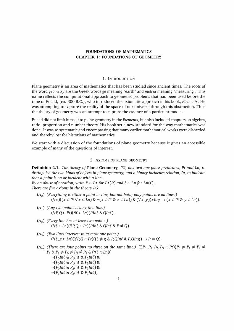
4. FINITE GEOMETRIES
Next we turn to finite geometries, ones with only finitely many points and lines. To get the theoryof the finite projective plane of order q, denoted PG(q), in addition to the five axioms given above,we add two more:(A5(q)) Every line contains exactly q+ 1 points.(A6(q)) Every point lies on exactly q+ 1 lines.The first geometry we look at is the finite projective plane of order 2, PG(2), also known as theFano Plane.
Theorem 4.1. The theory PG(2) consisting of PG together with the two axioms (5)2 and (6)2determines a finite geometry of seven points and seven lines, called the Fano plane.
Proof. See Exercise ?? to prove from the axioms and Exercise ?? that the following diagram givesa model of PG(2) and that any model must have the designated number of points and lines. ⇤
A
B
C
D
E
F
G
Next we construct a different model of this finite geometry using a vector space. The vector spaceunderlying the construction is the vector space of dimension three over the field of two elements,Z2 = {0, 1}. The points of the geometry are one dimensional subspaces. Since a one-dimensional

4 FOUNDATIONS OF MATHEMATICS CHAPTER 1: FOUNDATIONS OF GEOMETRY
subspace of Z2 has exactly two triples in it, one of which is the triple (0,0,0), we identify thepoints with the triples of 0’s and 1’s that are not all zero. The lines of the geometry are the twodimensional subspaces. The incidence relation is determined by a point is on a line if the onedimensional subspace is a subspace of the two dimensional subspace. Since a two dimensionalsubspace is picked out as the orthogonal complement of a one- dimensional subspace, each twodimensional subspace is identified with the non-zero triple, and to test if point (i, j, k) is on line[`, m, n], one tests the condition
i`+ jm+ kn⌘ 0 (mod 2).
There are exactly 23 = 8 ordered triples of 0’s and 1’s, of which one is the all zero vector. Thusthe ordered triples pick out the correct number of points and lines. The following array gives theincidence relation, and allows us to check that there are three points on every line and three linesthrough every point.
In [1,0,0] [0,1,0] [0,0,1] [1,1,0] [1,0,1] [0,1,1] [1,1,1]
(1,0,0) 0 1 1 0 0 1 0(0,1,0) 1 0 1 0 1 0 0(0,0,1) 1 1 0 1 0 0 0(1,1,0) 0 0 1 1 0 0 1(1,0,1) 0 1 0 0 1 0 1(0,1,1) 1 0 0 0 0 1 1(1,1,1) 0 0 0 1 1 1 0
The vector space construction works over other finite fields as well. The next bigger example isthe projective geometry of order 3, PG(3). The points are the one dimensional subspaces of thevector space of dimension 3 over the field of three elements, Z3 = {0,1,2}. This vector spacehas 33 � 1 = 27� 1 = 26 non-zero vectors. Each one dimensional subspace has two non-zeroelements, so there are 26/2 = 13 points in the geometry. As above, the lines are the orthogonal orperpendicular complements of the subspaces that form the lines, so there are also 13 of them. Thetest for incidence is similar to the one above, except that one must work (mod 3) rather than(mod 2).This construction works for each finite field. In each case the order of the projective geometry isthe size of the field.The next few lemmas list a few facts about projective planes.
Lemma 4.2. In any model of PG(q), any two lines intersect in a point.
Lemma 4.3. In any model of PG(q) there are exactly q
2 + q+ 1 points.
Lemma 4.4. In any model of PG(q) there are exactly q
2 + q+ 1 lines.
For models built using the vector space construction over a field of q elements, it is easy to computethe number of points and lines as q
3�1q�1 = q
2 + q+ 1. However there are non-isomorphic projectiveplanes of the same order. For a long time four non-isomorphic planes of order nine were known,each obtained by a variation on the above vector space construction. Recently it has been shownwith the help of a computer that there are exactly four non-isomorphic planes of order nine.Since the order of a finite field is always a prime power, the models discussed so far all haveprime power order. Much work has gone into the search for models of non-prime power order. Awell-publicized result showed that there were no projective planes of order 10. This proof requiredmany hours of computer time.

FOUNDATIONS OF MATHEMATICSCHAPTER 2: PROPOSITIONAL LOGIC
1. THE BASIC DEFINITIONS
Propositional logic concerns relationships between sentences built up from primitive propositionsymbols with logical connectives.
The symbols of the language of predicate calculus are(1) Logical connectives: ¬, & , _,!,$(2) Punctuation symbols: ( , )(3) Propositional variables: A0, A1, A2, . . . .
A propositional variable is intended to represent a proposition which can either be true or false.Restricted versions, L , of the language of propositional logic can be constructed by specifying asubset of the propositional variables. In this case, let PVar(L ) denote the propositional variablesof L .
Definition 1.1. The collection of sentences, denoted Sent(L ), of a propositional languageL is definedby recursion.
(1) The basis of the set of sentences is the set PVar(L ) of propositional variables of L .(2) The set of sentences is closed under the following production rules:
(a) If A is a sentence, then so is (¬A).(b) If A and B are sentences, then so is (A & B).(c) If A and B are sentences, then so is (A_ B).(d) If A and B are sentences, then so is (A! B).(e) If A and B are sentences, then so is (A$ B).
Notice that as long as L has at least one propositional variable, then Sent(L ) is infinite. Whenthere is no ambiguity, we will drop parentheses.
In order to use propositional logic, we would like to give meaning to the propositional variables.Rather than assigning specific propositions to the propositional variables and then determiningtheir truth or falsity, we consider truth interpretations.
Definition 1.2. A truth interpretation for a propositional language L is a function
I : PVar(L )! {0, 1 } .If I(Ai) = 0, then the propositional variable Ai is considered represent a false proposition under thisinterpretation. On the other hand, if I(Ai) = 1, then the propositional variable Ai is considered torepresent a true proposition under this interpretation.
There is a unique way to extend the truth interpretation to all sentences of L so that theinterpretation of the logical connectives reflects how these connectives are normally understoodby mathematicians.
1
2 FOUNDATIONS OF MATHEMATICS CHAPTER 2: PROPOSITIONAL LOGIC
Definition 1.3. Define an extension of a truth interpretation I : PVar(L )! {0,1 } for a propositionallanguage to the collection of all sentences of the language by recursion:
(1) On the basis of the set of sentences, PVar(L ), the truth interpretation has already beendefined.
(2) The definition is extended to satisfy the following closure rules:(a) If I(A) is defined, then I(¬A) = 1� I(A).(b) If I(A) and I(B) are defined, then I(A & B) = I(A) · I(B).(c) If I(A) and I(B) are defined, then I(A_ B) = max { I(A), I(B) }.(d) If I(A) and I(B) are defined, then
I(A! B) =
(0 if I(A) = 1 and I(B) = 0,
1 otherwise.(1)
(e) If I(A) and I(B) are defined, then I(A$ B) = 1 if and only if I(A) = I(B).
Intuitively, tautologies are statements which are always true, and contradictions are ones whichare never true. These concepts can be defined precisely in terms of interpretations.
Definition 1.4. A sentence' is a tautology for a propositional languageL if every truth interpretationI has value 1 on ', I(') = 1. ' is a contradiction if every truth interpretation I has value 0 on', I(') = 0. Two sentences ' and are logically equivalent, in symbols ', , if every truthinterpretation I takes the same value on both of them, I(') = I( ). A sentence ' is satisfiable ifthere is some truth interpretation I with I(') = 1.
The notion of logical equivalence is an equivalence relation; that is, it is a reflexive, symmetricand transitive relation. The equivalence classes given by logical equivalence are infinite for non-trivial languages (i.e., those languages containing at least one propositional variable). However,if the language has only finitely many propositional variables, then there are only finitely manyequivalence classes.
Notice that ifL has n propositional variables, then there are exactly d = 2n truth interpretations,which we may list as I = { I0, I1, . . . , Id�1 }. Since each Ii maps the truth values 0 or 1 to each ofthe n propositional variables, we can think of each truth interpretation as a function from the set{0, . . . , n� 1} to the set {0,1}. The collection of such functions can be written as {0,1}n, whichcan also be interpreted as the collection of binary strings of length n.
Each sentence ' gives rise to a function T F' : I ! {0, 1 } defined by T F'(Ii) = Ii(').Informally, T F' lists the column under ' in a truth table. Note that for any two sentences ' and , if T F' = T F then ' and are logically equivalent. Thus there are exactly 2d = 22n
manyequivalence classes.
Lemma 1.5. The following pairs of sentences are logically equivalent as indicated by the metalogicalsymbol,:
(1) ¬¬A , A.(2) ¬A_¬B , ¬(A & B).(3) ¬A & ¬B , ¬(A_ B).(4) A! B , ¬A_ B.(5) A$ B , (A! B) & (B! A).
Proof. Each of these statements can be proved using a truth table, so from one example the readermay do the others. Notice that truth tables give an algorithmic approach to questions of logicalequivalence.

FOUNDATIONS OF MATHEMATICS CHAPTER 2: PROPOSITIONAL LOGIC 3
A B (¬A) (¬B) ((¬A)_ (¬B)) (A & B) (¬(A & B))
I0 0 0 1 1 1 0 1I1 1 0 0 1 1 0 1I2 0 1 1 0 1 0 1I3 1 1 0 0 0 1 0
" "⇤
Using the above equivalences, one could assume that ¬ and _ are primitive connectives, anddefine the others in terms of them. The following list gives three pairs of connectives each of whichis sufficient to get all our basic list:
¬,_¬, &¬,!
In logic, the word “theory” has a technical meaning, and refers to any set of statements, whethermeaningful or not.
Definition 1.6. A set � of sentences in a language L is satisfiable if there is some interpretation Iwith I(') = 1 for all ' 2 � . A set of sentences � logically implies a sentence ', in symbols, � |= 'if for every interpretation I, if I( ) = 1 for all 2 � , then I(') = 1. A (propositional) theory in alanguage L is a set of sentences � ✓ Sent(L ) which is closed under logical implication.
Notice that a theory as a set of sentences matches with the notion of the theory of plane geometryas a set of axioms. In studying that theory, we developed several models. The interpretations playthe role here that models played in that discussion. Here is an example of the notion of logicalimplication defined above.
Lemma 1.7. { (A & B), (¬C) } |= (A_ B).
2. DISJUNCTIVE NORMAL FORM THEOREM
In this section we will show that the language of propositional calculus is sufficient to representevery possible truth function.
Definition 2.1.(1) A literal is either a propositional variable Ai or its negation ¬Ai.(2) A conjunctive clause is a conjunction of literals and a disjunctive clause is a disjunction of
literals. We will assume in each case that each propositional variable occurs at most once.(3) A propositional sentence is in disjunctive normal form if it is a disjunction of conjunctive
clauses and it is in conjunctive normal form if it is a conjunction of disjunctive clauses.
Lemma 2.2.(i) For any conjunctive clause C = �(A1, . . . , An), there is a unique interpretation IC : {A1, . . . , An}!{0, 1} such that IC(�) = 1.
(ii) Conversely, for any interpretation I : {A1, . . . , An} ! {0,1}, there is a unique conjunctiveclause CI (up to permutation of literals) such that I(CI ) = 1 and for any interpretation J 6= I ,J(CI ) = 0.

4 FOUNDATIONS OF MATHEMATICS CHAPTER 2: PROPOSITIONAL LOGIC
Proof. (i) Let
Bi =⇢
Ai if C contains Ai as a conjunct¬Ai if C contains ¬Ai as a conjunct
.
It follows that C = B1 & . . . & Bn. Now let IC (Ai) = 1 if and only if Ai = Bi . Then clearly I(Bi) = 1for i = 1, 2, . . . , n and therefore IC (C) = 1. To show uniqueness, if J(C) = 1 for some interpretationJ , then �(Bi) = 1 for each i and hence J = IC .
(ii) Let
Bi =⇢
Ai if I(Ai) = 1¬Ai if I(Ai) = 0
.
Let CI = B1 & . . . & Bn. As above I(CI ) = 1 and J(CI ) = 1 implies that J = I .It follows as above that I is the unique interpretation under which CI is true. We claim that CI
is the unique conjunctive clause with this property. Suppose not. Then there is some conjunctiveclause C 0 such that I(C 0) = 1 and C 0 6= CI . This implies that there is some literal Ai in C 0 and ¬Aiin CI (or vice versa). But I(C 0) = 1 implies that I(Ai) = 1 and I(CI) = 1 implies that I(¬Ai) = 1,which is clearly impossible. Thus CI is unique. ⇤
Here is the Disjunctive Normal Form Theorem.
Theorem 2.3. For any truth function F : {0, 1}n! {0, 1}, there is a sentence � in disjunctive normalform such that F = T F� .
Proof. Let I1, I2, . . . , Ik be the interpretations in {0,1}n such that F(Ii) = 1 for i = 1, . . . , k. Foreach i, let Ci = CIi
be the conjunctive clauses guaranteed to hold by the previous lemma. Now let� = C1 _ C2 _ . . . _ Ck. Then for any interpretation I ,
T F�(I) = 1 if and only if I(�) = 1 (by definition)
if and only if I(Ci) = 1 for some i = 1, . . . , k
if and only if I = Ii for some i (by the previous lemma)
if and only if F(I) = 1 (by the choice of I1, . . . , Ik)
Hence T F� = F as desired. ⇤Example 2.4. Suppose that we want a formula �(A1, A2, A3) such that I(�) = 1 only for the threeinterpretations (0,1, 0), (1,1, 0) and (1,1, 1). Then
� = (¬A1 & A2 & ¬A3)_ (A1 & A2 & ¬A3)_ (A1 & A2 & A3).
It follows that the connectives ¬,&,_ are sufficient to express all truth functions. By thedeMorgan laws (2,3 of Lemma 2.5) ¬,_ are sufficient and ¬,^ are also sufficient.
3. PROOFS
One of the basic tasks that mathematicians do is proving theorems. This section develops thePropositional Calculus, which is a system rules of inference for propositional languages. With itone formalizes the notion of proof. Then one can ask questions about what can be proved, whatcannot be proved, and how the notion of proof is related to the notion of interpretations.
The basic relation in the Propositional Calculus is the relation proves between a set, � ofsentences and a sentence B. A more long-winded paraphrase of the relation “� proves B” is “there
FOUNDATIONS OF MATHEMATICS CHAPTER 2: PROPOSITIONAL LOGIC 5
is a proof of B using what ever hypotheses are needed from � ”. This relation is denoted X ` Y ,with the following abbreviations for special cases:
Formal Version: � ` {B } {A} ` B ; ` B
Abbreviation: � ` B A` B ` B
Let ? be a new symbol that we will add to our propositional language. The intended interpre-tation of ? is ‘falsehood,’ akin to asserting a contradiction.
Definition 3.1. A formal proof or derivation of a propositional sentence � from a collection ofpropositional sentences � is a finite sequence of propositional sentences terminating in � where eachsentence in the sequence is either in � or is obtained from sentences occurring earlier in the sequenceby means of one of the following rules.
(1) (Given rule) Any B 2 � may be derived from � in one step.(2) (&-Elimination) If (A & B) has been derived from � then either of A or B may be derived from� in one further step.
(3) (_-Elimination) If (A_ B) has been derived from � , under the further assumption of A we canderive C from � , and under the further assumption of B we can derive C from � , then we canderive C from � in one further step.
(4) (!-Elimination) If (A! B) and A have been derived from � , then B can be derived from � inone further step.
(5) (?-Elimination) If ? has been deduced from � , then we can derive any sentence A from � inone further step.
(6) (¬-Elimination) If ¬¬A has been deduced from � , then we can derive A from � in one furtherstep.
(7) (&-Introduction) If A and B have been derived from � , then (A & B) may be derived from � inone further step.
(8) (_-Introduction) If A has been derived from � , then either of (A_ B), (B _ A) may be derivedfrom � in one further step.
(9) (!-Introduction) If under the assumption of A we can derive B from � , then we can deriveA! B from � in one further step.
(10) (?-Introduction) If (A & ¬A) has been deduced from � , then we can derive ? from � in onefurther step.
(11) (¬-Introduction) If ? has been deduced from � and A, then we can derive ¬A from � in onefurther step.
The relation � ` A can now be defined to hold if there is a formal proof of A from � that usesthe rules given above. The symbol ` is sometimes called a (single) turnstile. Here is a more precise,formal definition.
Definition 3.2. The relation � ` B is the smallest subset of pairs (� , B) from P (Sent)⇥ Sent whichcontains every pair (� , B) such that B 2 � and is closed under the above rules of deduction.
We now provide some examples of proofs.
Proposition 3.3. For any sentences A, B, C(1) ` A! A

6 FOUNDATIONS OF MATHEMATICS CHAPTER 2: PROPOSITIONAL LOGIC
(2) A! B ` ¬B! ¬A
(3) {A! B, B! C} ` A! C
(4) A` A_ B and A` B _ A
(5) {A_ B,¬A} ` B
(6) A_ A` A
(7) A` ¬¬A
(8) A_ B ` B _ A and A & B ` B & A
(9) (A_ B)_ C ` A_ (B _ C) and A_ (B _ C) ` (A_ B)_ C
(10) (A & B) & C ` A & (B & C) and A & (B & C) ` (A & B) & C
(11) A & (B _ C) ` (A & B)_ (A & C) and (A & B)_ (A & C) ` A & (B _ C
(12) A_ (B & C) ` (A_ B) & (A_ C) and (A_ B) & (A_ C) ` A_ (B & C)(13) ¬(A & B) ` ¬A_¬B and ¬A_¬B ` ¬(A & B)(14) ¬(A_ B) ` ¬A & ¬B and ¬A & ¬B ` ¬(A_ B)(15) ¬A_ B ` A! B and A! B ` ¬A_ B
(16) ` A_¬A
We give brief sketches of some of these proofs to illustrate the various methods.
Proof.
1. ` A! A
1 A Assumption
2 A Given
3 A! A !-Introduction (1-2)
3. {A! B, B! C} ` A! C
1 A! B Given
2 B! C Given
3 A Assumption
4 B !-Elimination 1,3
5 C !-Elimination 2,4
6 A! C !-Introduction 3-5
4. A` A_ B and A` B _ A
1 A Given
2 A_ B _-Introduction 1
FOUNDATIONS OF MATHEMATICS CHAPTER 2: PROPOSITIONAL LOGIC 7
1 A Given
2 B _ A _-Introduction 1
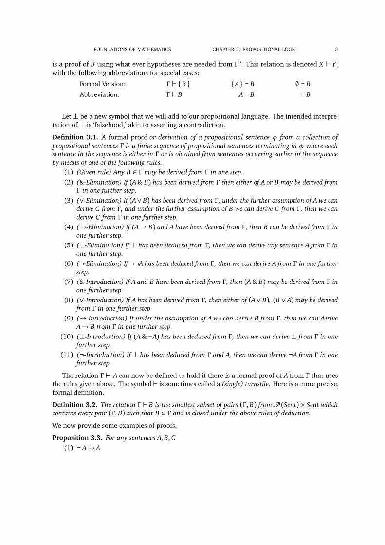
5. {A_ B,¬A} ` B
1 A_ B Given
2 ¬A Given
3 A Assumption
4 A & ¬A & -Introduction 2,3
5 ? ?-Introduction 4
6 B ?-Elimination 5
7 B Assumption
8 B Given
9 B _-Elimination 1-8
6. A_ A` A
1 A_ A Given
2 A Assumption
3 A Given
4 A Assumption
5 A Given
6 A _-Elimination 1-5
7. A` ¬¬A
1 A Given
2 ¬A Assumption
3 A & ¬A &-Introduction 1,2
4 ? ?-Introduction 3
5 ¬¬A ¬-Introduction 1-4
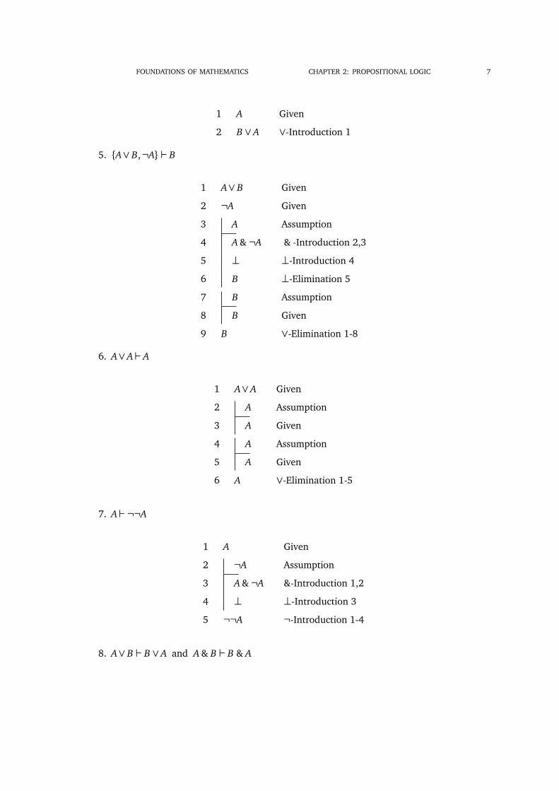
8. A_ B ` B _ A and A & B ` B & A
8 FOUNDATIONS OF MATHEMATICS CHAPTER 2: PROPOSITIONAL LOGIC
1 A_ B Given
2 A Assumption
3 B _ A _-Introduction 2
4 B Assumption
5 B _ A _-Introduction 2
6 B _ A _-Elimination 1-5
1 A & B Given
2 A &-Elimination
3 B &-Elimination
4 B & A &-Introduction 2-3
10. (A & B) & C ` A & (B & C) and A & (B & C) ` (A & B) & C
1 (A & B) & C Given
2 A & B &-Elimination 1
3 A &-Elimination 2
4 B &-Elimination 2
5 C &-Elimination 1
6 B & C &-Introduction 4,5
7 A & (B & C) &-Introduction 3,6
13. ¬(A & B) ` ¬A_¬B and ¬A_¬B ` ¬(A & B)

FOUNDATIONS OF MATHEMATICS CHAPTER 2: PROPOSITIONAL LOGIC 9
1 ¬(A & B) Given
2 A_¬A Item 6
3 ¬A Assumption
4 ¬A_¬B _-Introduction 4
5 A Assumption
6 B _¬B Item 6
7 ¬B Assumption
8 ¬A_¬B _-Introduction 7
9 B Assumption
10 A & B & -Introduction 5,9
11 ? ?-Introduction 1,10
12 ¬A_¬B Item 5
13 ¬A_¬B _-Elimination 6-12
14 ¬A_¬B _-Elimination 2-13
1 ¬A_¬B Given
2 A & B Assumption
3 A & -Elimination 2
4 ¬¬A Item 8, 3
5 ¬B Disjunctive Syllogism 1,4
6 B & -Elimination 2
7 ? ?-Introduction 5,6
8 ¬(A & B) Proof by Contradiction 2-7
15. ¬A_ B ` A! B and A! B ` ¬A_ B
1 ¬A_ B Given
2 A Assumption
3 ¬¬A Item 8, 2
4 B Item 5 1,3
5 A! B !-Introduction 2-4

10 FOUNDATIONS OF MATHEMATICS CHAPTER 2: PROPOSITIONAL LOGIC
1 A! B Given
2 ¬(¬A_ B) Assumption
3 ¬¬A & ¬B Item 14, 1
4 ¬¬A &-Introduction 3
5 A ¬-Elimination 4
6 B !-Elimination 1,5
7 ¬B &-Introduction 3
8 B & ¬B &-Introduction 6,7
9 ? ?-Introduction 8
10 ¬A_ B ?-Elimination 2-9
16. ` A_¬A
1 ¬(A_¬A) Assumption
2 ¬A & ¬¬A Item 14, 1
3 ? ?-Introduction 3
4 ¬A_ A ¬_-Rule (1-2)
⇤The following general properties about ` will be useful when we prove the soundness and
completeness theorems.
Lemma 3.4. For any sentences A and B, if � ` A and � [ {A} ` B, then � ` B.
Proof. � [ {A} ` B implies � ` A! B by!-Introduction. Combining this latter fact with the factthat � ` A yields � ` B by!-Elimination. ⇤Lemma 3.5. If � ` B and � ✓�, then � ` B.
Proof. This follows by induction on proof length. For the base case, if B follows from � on the basisof the Given Rule, then it must be the case that B 2 � . Since � ⇢� it follows that B 2� and hence� ` B by the Given Rule.
If the final step in the proof of B from � is made on the basis of any one of the rules, then wemay assume by the induction hypothesis that the other formulas used in these deductions followfrom � (since they follow from � ). We will look at two cases and leave the rest to the reader.
Suppose that the last step comes by!-Elimination, where we have derived A! B and A from� earlier in the proof. Then we have � ` A! B and � ` B. By the induction hypothesis, � ` A and� ` A! B. Hence � ` B by!-Elimation.
Suppose that the last step comes from &-Elimination, where we have derived A & B from �earlier in the proof. Since � ` A & B, by inductive hypothesis it follows that � ` A & B. Hence� ` B by &-elimination. ⇤
Next we prove a version of the Compactness Theorem for our deduction system.
FOUNDATIONS OF MATHEMATICS CHAPTER 2: PROPOSITIONAL LOGIC 11
Theorem 3.6. If � ` B, then there is a finite set �0 ✓ � such that �0 ` B.
Proof. Again we argue by induction on proofs. For the base case, if B follows from � on the basisof the Given Rule, then B 2 � and we can let �0 = {B}.
If the final step in the proof of B from � is made on the basis of any one of the rules, then wemay assume by the induction hypothesis that the other formulas used in these deductions followfrom some finite �0 ✓ � . We will look at two cases and leave the rest to the reader.
Suppose that the last step of the proof comes by _-Introduction, so that B is of the form C _ D.Then, without loss of generality, we can assume that we derived C from � earlier in the proof.Thus � ` C . By the induction hypothesis, there is a finite �0 ✓ � such that �0 ` C . Hence by_-Introduction, �0 ` C _ D.
Suppose that the last step of the proof comes by _-Elimination. Then earlier in the proof(i) we have derived some formula C _ D from � ,
(ii) under the assumption of C we have derived B from � , and(iii) under the assumption of D we have derived B from � .
Thus, � ` C _ D, � [ {C} ` B, and � [ {D} ` B. Then by assumption, by the induction hypothesis,there exist finite sets �0, �1, and �2 of � such that �0 ` C _ D, �1 [ {C} ` B and �2 [ {D} ` B. ByLemma 3.5,
(i) �0 [ �1 [ �2 ` C _ D(ii) �0 [ �1 [ �2 [ {C} ` B
(iii) �0 [ �1 [ �2 [ {D} ` BThus by _-Elimination, we have �0 [ �1 [ �2 ` B. Since �0 [ �1 [ �2 is finite and �0 [ �1 [ �2 ✓ � , theresult follows. ⇤
4. THE SOUNDNESS THEOREM
We now determine the precise relationship between ` and |= for propositional logic. Our firstmajor theorem says that if one can prove something in A from a theory � , then � logically impliesA.
Theorem 4.1 (Soundness Theorem). If � ` A, then � |= A.
Proof. The proof is by induction on the length of the deduction of A. We need to show that if thereis a proof of A from � , then for any interpretation I such that I(�) = 1 for all � 2 � , I(A) = 1.
(Base Case): For a one-step deduction, we must have used the Given Rule, so that A2 � . Ifthe truth interpretation I has I(�) = 1 for all � 2 � , then of course I(A) = 1 since A2 � .
(Induction): Assume the theorem holds for all shorter deductions. Now proceed by cases onthe other rules. We prove a few examples and leave the rest for the reader.
Suppose that the last step of the deduction is given by _-Introduction, so that A has the formB _ C . Without loss of generality, suppose we have derived B from � earlier in the proof. Supposethat I(�) = 1 for all � 2 � . Since the proof of � ` B is shorter than the given deduction of B_ C , bythe inductive hypothesis, I(B) = 1. But then I(B _ C) = 1 since I is an interpretation.
Suppose that the last step of the deduction is given by &-Elimination. Suppose that I(�) = 1for all � 2 � . Without loss of generality A has been derived from a sentence of the form A & B,which has been derived from � in a strictly shorter proof. Since � ` A & B, it follows by inductivehypothesis that � |= A & B, and hence I(A & B) = 1. Since I is an interpretation, it follows thatI(A) = 1.

12 FOUNDATIONS OF MATHEMATICS CHAPTER 2: PROPOSITIONAL LOGIC
Suppose that the last step of the deduction is given by!-Introduction. Then A has the formB! C . It follows that under the assumption of B, we have derived C from � . Thus � [ {B} ` C ina strictly shorter proof. Suppose that I(�) = 1 for all � 2 � . We have two cases to consider.
Case 1: If I(B) = 0, it follows that I(B! C) = 1.Case 2: If I(B) = 1, then since � [ {B} ` C ,
it follows that I(C) = 1. Then I(B! C) = 1. In either case, the conclusion follows.⇤
Now we know that anything we can prove is true. We next consider the contrapositive of theSoundness Theorem.
Definition 4.2. A set � of sentences is consistent if there is some sentence A such that � 0 A; otherwise� is inconsistent.
Lemma 4.3. � of sentences is inconsistent if and only if there is some sentence A such that � ` A and� ` ¬A.
Proof. Suppose first that � is inconsistent. Then by definition, � ` � for all formulas � and hence� ` A and � ` ¬A for every sentence A.
Next suppose that, for some A, � ` A and � ` ¬A. It follows by &-Introduction that � ` A & ¬A.By ?-Introduction, � ` ?. Then by ?-Elimination, for each �, � ` �. Hence � is inconsistent. ⇤Proposition 4.4. If � is satisfiable, then it is consistent.
Proof. Assume that � is satisfiable and let I be an interpretation such that I(�) = 1 for all � 2 � .Now suppose by way of contradiction that � is not consistent. Then there is some sentence A suchthat � ` A and � ` ¬A. By the Soundness Theorem, � |= A and � |= ¬A. But then I(A) = 1 andI(¬A) = 1 which is impossible since I is an interpretation. This contradiction demonstrates that �is consistent. ⇤
In Section 5, we will prove the converse of the Soundness Theorem by showing that anyconsistent theory is satisfiable.
5. THE COMPLETENESS THEOREM
Theorem 5.1. (The Completeness Theorem, Version I) If � |= A, then � ` A.
Theorem 5.2. (The Completeness Theorem, Version II) If � is consistent, then � is satisfiable.
We will show that Version II implies Version I and then prove Version II. First we give alternateversions of the Compactness Theorem (Theorem 3.6).
Theorem 5.3. (Compactness Theorem, Version II). If every finite subset of � is consistent, then � isconsistent.
Proof. We show the contrapositive. Suppose that� is not consistent. Then, for some B,� ` B & ¬B.It follows from Theorem 3.6 that � has a finite subset �0 such that �0 ` B & ¬B. But then �0 isnot consistent. ⇤Theorem 5.4. (Compactness Theorem, Version III). Suppose that
(i) � =S
n�n,(ii) �n ✓�n+1 for every n, and
(iii) �n is consistent for each n.
FOUNDATIONS OF MATHEMATICS CHAPTER 2: PROPOSITIONAL LOGIC 13
Then � is consistent.
Proof. Again we show the contrapositive. Suppose that � is not consistent. Then by Theorem 5.4,� has a finite, inconsistent subset F = {�1,�2, . . . ,�k}. Since � =
Sn�n, there exists, for each
i k, some ni such that �i 2�i . Letting n =max{ni : i k}, it follows from the fact that the � j ’sare inconsistent that F ✓�n. But then �n is inconsistent. ⇤
Next we prove a useful lemma.
Lemma 5.5. For any � and A, � ` A if and only if � [ {¬A} is inconsistent.
Proof. Suppose first that � ` A. Then � [ {¬A} proves both A and ¬A and is therefore inconsistent.Suppose next that � [ {¬A} is inconsistent. It follows from ¬-Introduction that � ` ¬¬A. Then
by ¬-Elimination, � ` A. ⇤We are already in position to show that Version II of the Completeness Theorem implies Version
I. We show the contrapositive of the statement of Version 1; that is, we show � 6` A implies � 6|= A.Suppose it is not the case that � ` A. Then by Lemma 5.5, � [ {¬A} is consistent. Thus by VersionII, � [ {¬A} is satisfiable. Then it is not the case that � |= A.
We establish a few more lemmas.
Lemma 5.6. If � is consistent, then for any A, either � [ {A} is consistent or � [ {¬A} is consistent.
Proof. Suppose that � [ {¬A} is inconsistent. Then by the previous lemma, � ` A. Then, for any B,� [ {A} ` B if and only if � ` B. Since � is consistent, it follows that � [ {A} is also consistent. ⇤Definition 5.7. A set � of sentences is maximally consistent if it is consistent and for any sentence A,either A2� or ¬A2�.
Lemma 5.8. Let � be maximally consistent.(1) For any sentence A, ¬A2� if and only if A /2�.(2) For any sentence A, if � ` A, then A2�.
Proof. (1) If ¬A2�, then A /2� since � is consistent. If A /2�, then ¬A2� since � is maximallyconsistent.
(2) Suppose that � ` A and suppose by way of contradiction that A /2 �. Then by part (1),¬A2�. But this contradicts the consistency of �. ⇤Proposition 5.9. Let � be maximally consistent and define the function I : Sent! {0, 1} as follows.For each sentence B,
I(B) =
®1 if B 2�;
0 if B 62�.Then I is a truth interpretation and I(B) = 1 for all B 2�.
Proof. We need to show that I preserves the four connectives: ¬, _, & , and!. We will show thefirst three and leave the last an exercise.
(¬): It follows from the definition of I and Lemma 5.8 that I(¬A) = 1 if and only if ¬A2� ifand only if A /2� if and only if I(A) = 0.
(_): Suppose that I(A_ B) = 1. Then A_ B 2 �. We argue by cases. If A 2 �, then clearlymax{I(A), I(B)} = 1. Now suppose that A /2 �. Then by completeness, ¬A 2 �. It follows fromProposition 3.3(5) that � ` B. Hence B 2� by Lemma 5.8. Thus max{I(A), I(B)}= 1.

14 FOUNDATIONS OF MATHEMATICS CHAPTER 2: PROPOSITIONAL LOGIC
Next suppose that max{I(A), I(B)}= 1. Without loss of generality, I(A) = 1 and hence A2�.Then � ` A_ B by _-Introduction, so that A_ B 2� by Lemma 5.8 and hence I(A_ B) = 1.
(&): Suppose that I(A & B) = 1. Then A & B 2�. It follows from &-Elimination that � ` A and� ` B. Thus by Lemma 5.8, A2� and B 2�. Thus I(A) = I(B) = 1.
Next suppose that I(A) = I(B) = 1. Then A2� and B 2�. It follows from &-Introduction that� ` A & B and hence A & B 2�. Therefore I(A & B) = 1. ⇤
We now prove Version II of the Completeness Theorem.
Proof of Theorem 5.2. Let � be a consistent set of propositional sentences. Let A0, A1, . . . be anenumeration of the set of sentences. We will define a sequence �0 ✓�1 ✓ . . . and let � =
Sn�n.
We will show that � is a complete and consistent extension of � and then define an interpretationI = I� to show that � is satisfiable.�0 = � and, for each n,
�n+1 =
®�n [ {An}, if �n [ {An} is consistent
�n [ {¬An}, otherwise.
It follows from the construction that, for each sentence An, either An 2 �n+1 or ¬An 2 �n+1.Hence � is complete. It remains to show that � is consistent.
Claim 1: For each n, �n is consistent.
Proof of Claim 1: The proof is by induction. For the base case, we are given that�0 = � is consistent.For the induction step, suppose that �n is consistent. Then by Lemma 5.6, either �n [ {An} isconsistent, or �n[ {¬An} is consistent. In the first case, suppose that �n[ {An} is consistent. Then�n+1 = �n [ {An} and hence �n+1 is consistent. In the second case, suppose that �n [ {An} isinconsistent. Then �n+1 =�n [ {¬An} and hence �n+1 is consistent by Lemma 5.6.
Claim 2: � is consistent.
Proof of Claim 2: This follows immediately from the Compactness Theorem Version III.
It now follows from Proposition 5.9 that there is a truth interpretation I such that I(�) = 1 forall � 2�. Since � ✓�, this proves that � is satisfiable. ⇤
We note the following consequence of the proof of the Completeness Theorem.
Theorem 5.10. Any consistent theory � has a maximally consistent extension. ⇤
6. COMPLETENESS, CONSISTENCY AND INDEPENDENCE
For a given set of sentences � , we sometimes identify � with the theory Th(� ) = {B : � ` B}.Thus we can alternatively define � to be consistent if there is no sentence B such that � ` B and� ` ¬B. Moreover, let us say that � is complete if for every sentence B, either � ` B or � ` ¬B(Note that if � is maximally consistent, it follows that � is complete, but the converse need not hold.We say that a consistent set � is independent if � has no proper subset � such that Th(�) = Th(� );this means that � is minimal among the sets � with Th(�) = Th(� ).
For example, in the language L with three propositional variables A, B, C , the set {A, B, C} isclearly independent and complete.
Lemma 6.1. � is independent if and only if, for every B 2 � , it is not the case that � � {B} ` B.
Proof. Left to the reader. ⇤

FOUNDATIONS OF MATHEMATICS CHAPTER 2: PROPOSITIONAL LOGIC 15
Lemma 6.2.A set � of sentences is complete and consistent if and only if there is a unique interpretation I satisfiedby � .
Proof. Left to the reader. ⇤We conclude this chapter with several examples.
Example 6.3. Let L = {A0, A1, . . . }.(1) The set �0 = {A0, A0 & A1, A1 & A2, . . . } is complete but not independent.
— It is complete since �0 ` An for all n, which determines the unique truth interpretation Iwhere I(An) = 1 for all n.
— It is not independent since, for each n, (A0 & A1 · · · & An+1)! (A0 & · · · & An).
(2) The set �1 = {A0, A0! A1, A1! A2, . . . } is complete and independent.— It is complete since �0 ` An for all n, which determines the unique truth interpretation I
where I(An) = 1 for all n.— To show that �1 is independent, it suffice to show that, for each single formula An! An+1,
it is not the case that �1 � {An ! An+1} ` (An ! An+1). This is witnessed by theinterpetation I where I(Aj) = 1 if j n and I(Aj) = 0 if j > n.
(3) The set �2 = {A0 _ A1, A2 _ A3, A4 _ A5, . . . } is independent but not complete.— It is not complete since there are many different interpretations satisfied by �2. In
particular, one interpretation could make An true if and only if n is odd, and anothercould make An true if and only if n is even.
— It is independent since, for each n, we can satisfy every sentence of �2 except A2n _A2n+1by the interpretation I where I(Aj) = 0 exactly when j = 2n or j = 2n+ 1.
FOUNDATIONS OF MATHEMATICSCHAPTER 3: PREDICATE LOGIC
Propositional logic treats a basic part of the language of mathematics, building more complicatedsentences from simple with connectives. However it is inadequate as it stands to express the richnessof mathematics. Consider the axiom of the theory of Plane Geometry, PG, which expresses thefact that any two points belong to a line. We wrote that statement formally with two one-placepredicates, Pt for points and Ln for lines, and one two-place predicate, In for incidence as follows:
(8P,Q 2 Pt)(9` 2 Ln)((PIn`) & (QIn`)).
This axiom includes predicates and quantifies certain elements. In order to test the truth of it,one needs to know how to interpret the predicates Pt, Ln and In, and the individual elements P, Q,`. Notice that these elements are “quantified” by the quantifiers to “for every” and “there is . . .such that.” Predicate logic is an enrichment of propositional logic to include predicates, individualsand quantifiers, and is widely accepted as the standard language of mathematics.
1. THE LANGUAGE OF PREDICATE LOGIC
The symbols of the language of the predicate logic are(1) logical connectives, ¬, _, & ,!,$;(2) the equality symbol =;(3) predicate letters Pi for each natural number i;(4) function symbols Fj for each natural number j;(5) constant symbols ck for each natural number k;(6) individual variables v` for each natural number `;(7) quantifier symbols 9 (the existential quantifier) and 8 (the universal quantifer); and(8) punctuation symbols (, ).A predicate letter is intended to represent a relation. Thus each predicate letter P is n-ary for
some n, which means that we write P(v1, . . . , vn). Similarly, a function symbol also is n-ary forsome n.
We make a few remarks on the quantifiers:(a) (9x)� is read “there exists an x such that � holds.”(b) (8x)� is read “for all x , � holds.”(c) (8x)✓ may be thought of as an abbreviation for (¬(9x)(¬✓ )).
Definition 1.1. A countable first-order language is obtained by specifying a subset of the predicateletters, function symbols and constants.
One can also work with uncountable first-order languages, but aside from a few examples inChapter 4, we will primarily work with countable first-order languages. An example of a first-orderlanguage is the language of arithmetic.
Example 1.2. The language of arithmetic is specified by {<,+,⇥, 0, 1 }. Here < is a 2-place relation,+ and ⇥ are 2-place functions and 0, 1 are constants. Equality is a special 2-place relation that wewill include in every language.
1
2 FOUNDATIONS OF MATHEMATICS CHAPTER 3: PREDICATE LOGIC
We now describe how first-order sentences are built up from a given language L .
Definition 1.3. The set of terms in a language L , denoted Term(L ), is recursively defined by(1) each variable and constant is a term; and(2) if t1, . . . , tn are terms and F is an n-place function symbol, then F(t1, . . . , tn) is a term.
A constant term is a term with no variables.
Definition 1.4. Let L be a first-order language. The collection of L -formulas is defined by recursion.First, the set of atomic formulas, denoted Atom(L ), consists of formulas of one of the following forms:
(1) P(t1, . . . , tn) where P is an n-place predicate letter and t1, . . . , tn are terms; and(2) t1 = t2 where t1 and t2 are terms.
The set of L -formulas is closed under the following rules(3) If � and ✓ are L -formulas, then (� _ ✓ ) is an L -formula. (Similarly, (� & ✓ ), (�! ✓ ),(�$ ✓ ), are L -formulas.)
(4) If � is an L -formula, then (¬�) is an L -formula.(5) If � is an L -formula, then (9v)� is an L -formula (as is (8v)�).
An example of an atomic formula in the language of arithmetic
0+ x = 0.
An example of a more complicated formula in the language, of plane geometry is the statementthat every element either has a point incident with it or is incident with some line.
(8v)(9x)((xInv)_ (vInx)).
A variable v that occurs in a formula � becomes bound when it is placed in the scope of aquantifier, that is, (9v) is placed in front of �, and otherwise v is free. The concept of being freeover-rides the concept of being bound in the sense that if a formula has both free and boundoccurrences of a variable v, then v occurs free in that formula. The formal definition of bound andfree variables is given by recursion.
Definition 1.5. A variable v is free in a formula � if(1) � is atomic;(2) � is ( _ ✓ ) and v is free in whichever one of and ✓ in which it appears;(3) � is (¬ ) and v is free in ;(4) � is (9y) , v is free in and y is not v.
Example 1.6.(1) In the atomic formula x + 5= 12, the variable x is free.(2) In the formula (9x)(x + 5= 12), the variable x is bound.(3) In the formula (9x)[(x 2 <+) & (|x � 5|= 10)], the variable x is bound.
We will refer to an L -formula with no free variables as an L -sentence.
2. MODELS AND INTERPRETATIONS
In propositional logic, we used truth tables and interpretations to consider the possible truthof complex statements in terms of their simplest components. In predicate logic, to consider thepossible truth of complex statements that involve quantified variables, we need to introduce modelswith universes from which we can select the possible values for the variables.
Definition 2.1. Suppose that L is a first-order language with
FOUNDATIONS OF MATHEMATICS CHAPTER 3: PREDICATE LOGIC 3
(i) predicate symbols P1, P2, . . . ,(ii) function symbols F1, F2, . . . , and
(iii) constant symbols c1, c2, . . . .Then an L -structure A consists of
(a) a nonempty set A (called the domain or universe of A),(b) a relation PA
i on A corresponding to each predicate symbol Pi,(c) a function FA
i on A corresponding to each function symbol Fi, and(d) a element cAi 2 A corresponding to each constant symbol ci.
Each relation PAi requires the same number of places as Pi , so that PA
i is a subset of Ar for somefixed r ( called the arity of Ri .) In addition, each function FA
i requires the same number of placesas Fi , so that FA
i : Ar ! A for some fixed r (called the arity of Rj).
Definition 2.2. Given a L -structure A, an interpretation I into A is a function I from the variablesand constants of L into the universe A of A that respects the interpretations of the symbols in L . Inparticular, we have
(i) for each constant symbol c j, I(c j) = cAj ,(ii) for each function symbol Fi, if Fi has parity n and t1, . . . , tn are terms such that I(t1), I(t2), . . . I(tn)
have been defined, then
I(Fi(t1, . . . , tn)) = FAi (I(t1), . . . , I(tn)).
For any interpretation I and any variable or constant x and for any element b of the universe,let Ib/x be the interpretation defined by
Ib/x(z) =
®b if z = x ,
I(z) otherwise.
Definition 2.3. We define by recursion the relation that a structure A satisfies a formula � via aninterpretation I into A, denoted n A |=I �:
For atomic formulas, we have:(1) A |=I t = s if and only if I(t) = I(s);(2) A |=I Pi(t1, . . . , tn) if and only if PA
i (I(t1), . . . , I(tn)).
For formulas built up by the logical connectives we have:(3) A |=I (� _ ✓ ) if and only if A |=I � or A |=I ✓ ;(4) A |=I (� & ✓ ) if and only if A |=I � and A |=I ✓ ;(5) A |=I (�! ✓ ) if and only if A 6|=I � or A |=I ✓ ;(6) A |=I (¬�) if and only if A 6|=I �.
For formulas built up with quantifiers:(7) A |=I (9v)� if and only if there is an a in A such that A |=Ia/x
�;(8) A |=I (8v)� if and only if for every a in A, A |=Ia/x
�.
If A |=I � for every interpretation I , we will suppress the subscript I , and simply write A |= �.In this case we say that A is a model of �.
Example 2.4. LetL (GT ) be the language of group theory, which uses the symbols {+, 0 }. A structurefor this language is A = ({0, 1,2 } ,+ (mod 3), 0). Suppose we consider formulas of L (GT ) which onlyhave variables among x1, x2, x3, x4. Define an interpretation I by I(xi)⌘ i mod 3 and I(0) = 0.

4 FOUNDATIONS OF MATHEMATICS CHAPTER 3: PREDICATE LOGIC
(1) Claim: A 6|=I x1 + x2 = x4.We check this claim by computation. Note that I(x1) = 1, I(x2) = 2, I(x1+x2) = I(x1)+mod3I(x2) = 1+mod3 2= 0. On the other hand, I(x4) = 1 6= 0, so A 6|=I x1 + x2 = x4.
(2) Claim: A |= (9x2)(x1 + x2 = x4)Define J = I0/x2
. As above check that A |=J x1 + x2 = x4. Then by the definition of thesatisfaction of an existential formula, A |=I (9x2)(x1 + x2 = x4).
Theorem 2.5. For everyL -formula �, for all interpretations I , J , if I and J agree on all the variablesfree in �, then A |=I � if and only if A |=J �.
Proof. Left to the reader. ⇤Corollary 2.6. If � is an L -sentence, then for all interpretations I and J, we have A |=I � if andonly if A |=J �.
Remark 2.7. Thus for L -sentences, we drop the subscript which indicates the interpretation of thevariables, and we say simply A models �.
Definition 2.8. Let � be an L -formula.(i) � is logically valid if A |=I � for every L -structure A and every interpretation I into A.
(ii) � is satisfiable if there is some L -structure A and some interpretation I into A such thatA |=I �.
(iii) � is contradictory if � is not satisfiable.
Definition 2.9. A L -theory � is a set of L -sentences. An L -structure A is a model of an L -theory� if and only if A |= � for all � in � . In this case we also say that � is satisfiable.
Definition 2.10. For a set ofL -formulas � and anL -formula �, we write � |= � and say “� implies�,” if for all L -structures A and for all L -interpretations I, if A |=I � for all � in � , then A |=I �.
Thus if � is an L -theory and � an L -sentence, then � |= � means every model of � is also amodel of �.
The following definition will be useful to us in the next section.
Definition 2.11. Given a term t and an L -formula � with free variable x, we write �[t/x] toindicate the result of substituting the term t for each free occurrence of x in �.
Example 2.12. If� is the formula (9y)(y 6= x) is the formula, then�[y/x] is the formula (9y)(y 6=y), which we expect never to be true.
3. THE DEDUCTIVE CALCULUS
The Predicate Calculus is a system of axioms and rules which permit us to derive the truestatements of predicate logic without the use of interpretations. The basic relation in the PredicateCalculus is the relation proves between a set � ofL formulas and anL -formula�, which formalizesthe concept that � proves �. This relation is denoted � ` �. As a first step in defining this relation,we give a list of additional rules of deduction, which extend the list we gave for propositional logic.
Some of our rules of the predicate calculus require that we exercise some care in how wesubstitute variables into certain formulas. Let us say that �[t/x] is a legal substitution of t for x in� if no free occurrence of x in � occurs in the scope of a quantifier of any variable appearing in t.For instance, if � has the form (8y)�(x , y), where x is free, I cannot legally substitute y in for x ,since then y would be bound by the universal quantifier.

FOUNDATIONS OF MATHEMATICS CHAPTER 3: PREDICATE LOGIC 5
10. (Equality rule) For any term t, the formula t = t may be derived from � is one step.
11. (Term Substitution) For any terms t1, t2, . . . , tn, s1, s2, . . . , sn, and any function symbol F ,if each of the sentences t1 = s1, t2 = s2, . . . , tn = sn have been derived from � , then wemay derive F(t1, t2, . . . , tn) = F(s1, s2, . . . , sn) from � in one additional step.
12. (Atomic Formula Substitution) For any terms t1, t2, . . . , tn, s1, s2, . . . , sn and any atomicformula �, if each of the sentences t1 = s1, t2 = s2, . . . , tn = sn, and �(t1, t2, . . . , tn), havebeen derived from � , then we may derive �(s1, s2, . . . , sn) from � in one additional step.
13. (8-Elimination) For any term t, if �[t/x] is a legal substitution and (8x)� has beenderived from � , then we may derive �[t/x] from � in one additional step.
14. (9-Elimination) To show that � [ {(9x)�(x)} ` ✓ , it suffices to show � [ {�(y)}, where yis a new variable that does not appear free in any formula in � nor in ✓ .
15. (8-Introduction) Suppose that y does not appear free in any formula in � , in any temporaryassumption, nor in (8x)�. If �[y/x] has been derived from � , then we may derive (8x)�from � in one additional step.
16. (9-Introduction) If �[t/x] is a legal substitution and �[t/x] has been derived from � ,then we may derive (9x)� from � in one additional step.
We remark on three of the latter four rules. First, the reason for the restriction on substitutionin 8-Elimination is that we need to ensure that t does not contain any free variable that would bebecome bound when we substitute t for x in �. For example, consider the formula (8x)(9y)x < yin the language of arithmetic. Let � be the formula (9y)x < y , in which x is free but y is bound.Observe that if we substitute the term y for x in �, the resulting formula is (9y)y < y. Thus,from (8x)(9y)x < y we can derive, for instance, (9y)x < y or (9y)c < y, but we cannot derive(9y)y < y .
Second, the idea behind 9-Elimination is this: Suppose in the course of my proof I have derived(9x)�(x). Informally, I would like to use the fact that � holds of some x , but to do so, I need torefer to this object. So I pick an unused variable, say a, and use this as a temporary name to standfor the object satisfying �. Thus, I can write down �(a). Eventually in my proof, I will discard thistemporary name (usually by 9-Introduction).
Third, in 8-Introduction, if we think of the variable y as an arbitrary object, then when weshow that y satisfies �, we can conclude that � holds of every object. However, if y is free in apremise in � or a temporary assumption, it is not arbitrary. For example, suppose we begin with thestatement (9x)(8z)(x+z = z) in the language of arithmetic and suppose we derive (8z)(y+z = z)by 9-Elimination (where y is a temporary name). We are not allowed to apply 8-Introduction here,for otherwise we could conclude (8x)(8z)(x + z = z), an undesirable conclusion.
Definition 3.1. The relation � ` � is the smallest subset of pairs (� ,�) from P (Sent)⇥ Sent thatcontains every pair (� ,�) such that � 2 � or � is t = t for some term t, and which is closed underthe 15 rules of deduction.
As in Propositional Calculus, to demonstrate that � ` �, we construct a proof. The nextproposition exhibits several proofs using the new axiom and rules of predicate logic.
6 FOUNDATIONS OF MATHEMATICS CHAPTER 3: PREDICATE LOGIC
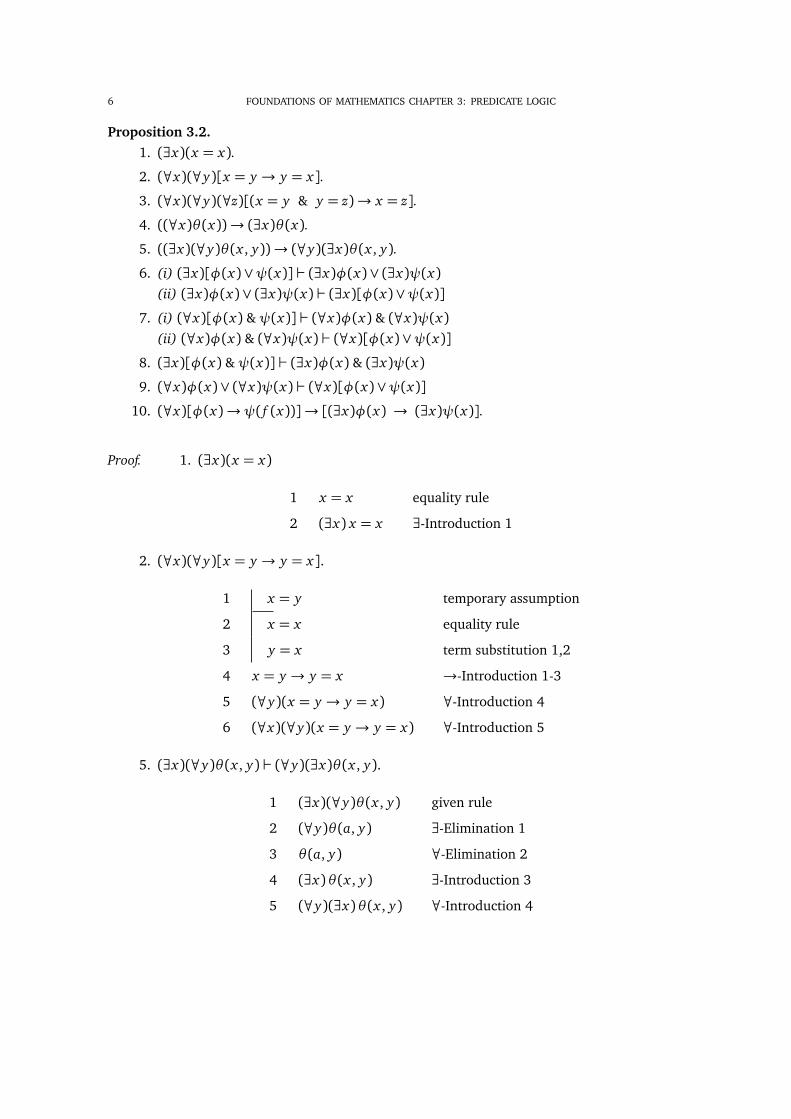
Proposition 3.2.1. (9x)(x = x).
2. (8x)(8y)[x = y ! y = x].
3. (8x)(8y)(8z)[(x = y & y = z)! x = z].
4. ((8x)✓ (x))! (9x)✓ (x).5. ((9x)(8y)✓ (x , y))! (8y)(9x)✓ (x , y).
6. (i) (9x)[�(x)_ (x)] ` (9x)�(x)_ (9x) (x)(ii) (9x)�(x)_ (9x) (x) ` (9x)[�(x)_ (x)]
7. (i) (8x)[�(x) & (x)] ` (8x)�(x) & (8x) (x)(ii) (8x)�(x) & (8x) (x) ` (8x)[�(x)_ (x)]
8. (9x)[�(x) & (x)] ` (9x)�(x) & (9x) (x)9. (8x)�(x)_ (8x) (x) ` (8x)[�(x)_ (x)]
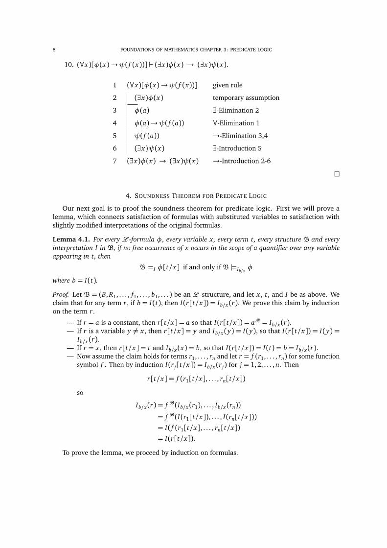
10. (8x)[�(x)! ( f (x))]! [(9x)�(x) ! (9x) (x)].
Proof. 1. (9x)(x = x)
1 x = x equality rule
2 (9x) x = x 9-Introduction 1
2. (8x)(8y)[x = y ! y = x].
1 x = y temporary assumption
2 x = x equality rule
3 y = x term substitution 1,2
4 x = y ! y = x !-Introduction 1-3
5 (8y)(x = y ! y = x) 8-Introduction 4
6 (8x)(8y)(x = y ! y = x) 8-Introduction 5
5. (9x)(8y)✓ (x , y) ` (8y)(9x)✓ (x , y).
1 (9x)(8y)✓ (x , y) given rule
2 (8y)✓ (a, y) 9-Elimination 1
3 ✓ (a, y) 8-Elimination 2
4 (9x)✓ (x , y) 9-Introduction 3
5 (8y)(9x)✓ (x , y) 8-Introduction 4

FOUNDATIONS OF MATHEMATICS CHAPTER 3: PREDICATE LOGIC 7
8. (9x)[�(x) & (x)] ` (9x)�(x) & (9x) (x)
1 (9x)[�(x) & (x)] given rule
2 �(a) & (a) 9-Elimination 1
3 �(a) &-Elimination 2
4 (9x)�(x) 9-Introduction 3
5 (a) &-Elimination 2
6 (9x) (x) 9-Introduction 5
7 (9x)�(x) & (9x) (x) &-Introduction 4,6
9. (8x)�(x)_ (8x) (x) ` (8x)[�(x)_ (x)]
1 (8x)�(x)_ (8x) (x) given rule
2 (8x)�(x) temporary assumption
3 �(x) 8-Elimination 2
4 �(x)_ (x) _-Introduction 3
5 (8x)[�(x)_ (x)] 8-Introduction 4
6 (8x) (x) temporary assumption
7 (x) 8-Elimination 6
8 �(x)_ (x) _-Introduction 7
9 (8x)[�(x)_ (x)] 8-Introduction 8
10 (8x)[�(x)_ (x)] _-Elimination 1-9
8 FOUNDATIONS OF MATHEMATICS CHAPTER 3: PREDICATE LOGIC
10. (8x)[�(x)! ( f (x))] ` (9x)�(x) ! (9x) (x).
1 (8x)[�(x)! ( f (x))] given rule
2 (9x)�(x) temporary assumption
3 �(a) 9-Elimination 2
4 �(a)! ( f (a)) 8-Elimination 1
5 ( f (a)) !-Elimination 3,4
6 (9x) (x) 9-Introduction 5
7 (9x)�(x) ! (9x) (x) !-Introduction 2-6
⇤
4. SOUNDNESS THEOREM FOR PREDICATE LOGIC
Our next goal is to proof the soundness theorem for predicate logic. First we will prove alemma, which connects satisfaction of formulas with substituted variables to satisfaction withslightly modified interpretations of the original formulas.
Lemma 4.1. For every L -formula �, every variable x, every term t, every structure B and everyinterpretation I in B, if no free occurrence of x occurs in the scope of a quantifier over any variableappearing in t, then
B |=I �[t/x] if and only if B |=Ib/x�
where b = I(t).
Proof. Let B = (B, R1, . . . , f1, . . . , b1, . . . ) be an L -structure, and let x , t, and I be as above. Weclaim that for any term r, if b = I(t), then I(r[t/x]) = Ib/x(r). We prove this claim by inductionon the term r.
— If r = a is a constant, then r[t/x] = a so that I(r[t/x]) = aB = Ib/x(r).— If r is a variable y 6= x , then r[t/x] = y and Ib/x(y) = I(y), so that I(r[t/x]) = I(y) =
Ib/x(r).— If r = x , then r[t/x] = t and Ib/x(x) = b, so that I(r[t/x]) = I(t) = b = Ib/x(r).— Now assume the claim holds for terms r1, . . . , rn and let r = f (r1, . . . , rn) for some function
symbol f . Then by induction I(r j[t/x]) = Ib/x(r j) for j = 1,2, . . . , n. Then
r[t/x] = f (r1[t/x], . . . , rn[t/x])
so
Ib/x(r) = f B (Ib/x(r1), . . . , Ib/x(rn))
= f B (I(r1[t/x]), . . . , I(rn[t/x]))= I( f (r1[t/x], . . . , rn[t/x])= I(r[t/x]).
To prove the lemma, we proceed by induction on formulas.

FOUNDATIONS OF MATHEMATICS CHAPTER 3: PREDICATE LOGIC 9
— For an atomic formula � of the form s1 = s2, we have
B |=I �[t/x],B |=I s1[t/x] = s2[t/x], I(s1[t/x]) = I(s2[t/x]), Ib/x(s1) = Ib/x(s2) (by the claim)
,B |=Ib/xs1 = s2
,B |=Ib/x�.
— For an atomic formula� of the form P(r1, . . . , rn), so that�[t/x] is P(r1[t/x], . . . , rn[t/x]),we have
B |=I �[t/x],B |=I P(r1[t/x], . . . , rn[t/x])
, PB (I(r1[t/x]), . . . , I(rn[t/x]))
, PB (Ib/x(r1), . . . , Ib/x(rn)) (by the claim)
,B |=Ib/xP(r1, . . . , rn)
,B |=Ib/x�.
— The inductive step forL -formulas is straightforward except for formulas of the form 8y�:Let be 8y�, where the Lemma holds for the formula �. Then
B |=I [t/x],B |=I 8y�[t/x],B |=Ia/y
�[t/x] (for each a 2 B)
,B |=(Ia/y )b/x � (by the inductive hypothesis)
,B |=(Ib/x )a/y� (for each a 2 B)
,B |=Ib/x8y�
,B |=Ib/x .
⇤
Theorem 4.2 (Soundness Theorem of Predicate Logic). If � ` �, then � |= �.
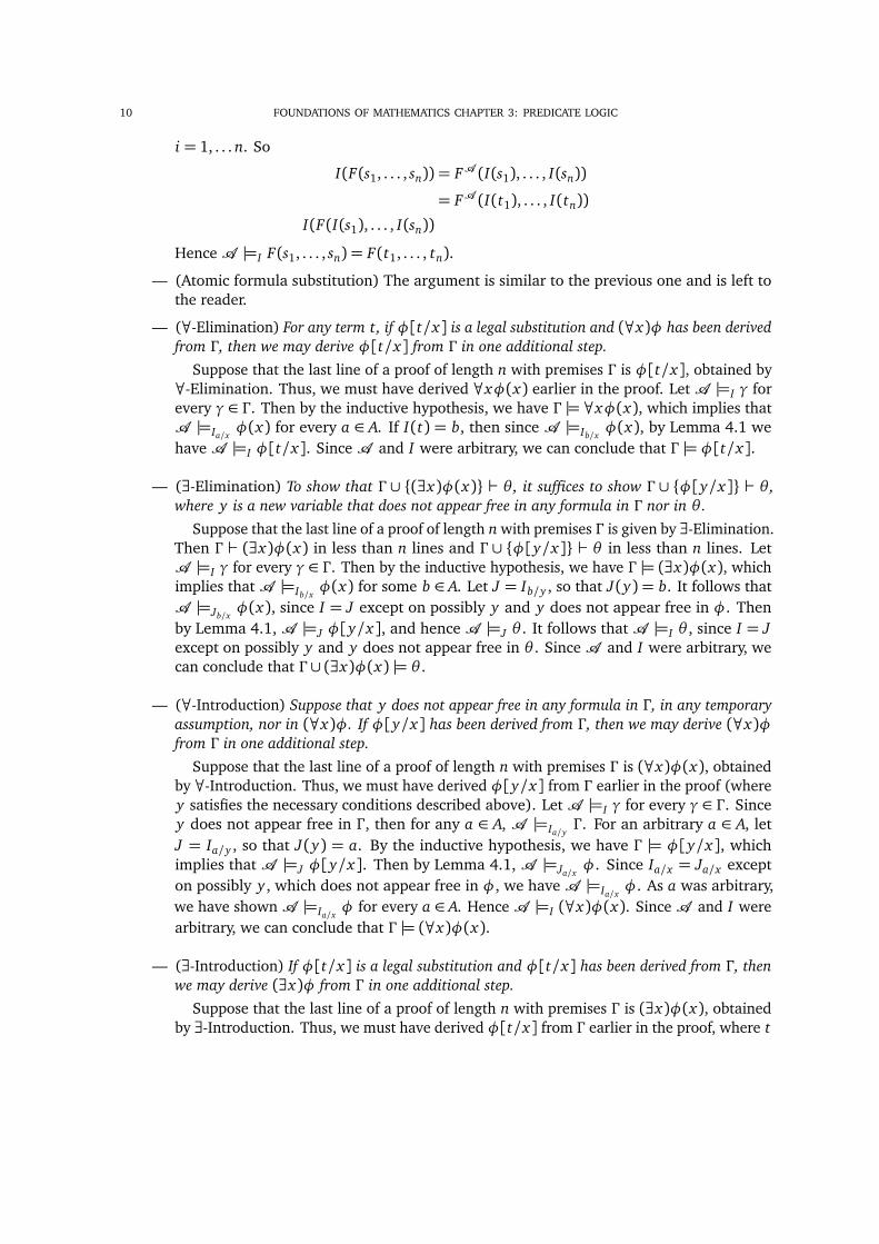
Proof. As in the proof of the soundness theorem for propositional logic, the proof is again byinduction on the length of the deduction of �. We need to show that if there is a proof of � from � ,then for any structureA and any interpretation I intoA , ifA |=I � for all � 2 � , thenA |=I �.The arguments for the rules from Propositional Logic carry over here, so we just need to verify theresult holds for the new rules.
Suppose the result holds for all formulas obtained in proofs of length strictly less than n lines.
— (Equality rule) Suppose the last line of a proof of length n with premises � is t = t forsome term t. SupposeA |=I � . Then since I(t) = I(t), we haveA |= t = t.
— (Term substitution) Suppose the last line of a proof of length n with premises � isF(s1, . . . , sn) = F(t1, . . . , tn), obtained by term substitution. Then we must have estab-lished s1 = t1, . . . , sn = tn earlier in the proof. By the inductive hypothesis, we must have� |= s1 = t1, . . . � |= sn = tn. Suppose thatA |=I � for every � 2 � . Then I(si) = I(ti) for
10 FOUNDATIONS OF MATHEMATICS CHAPTER 3: PREDICATE LOGIC
i = 1, . . . n. So
I(F(s1, . . . , sn)) = FA (I(s1), . . . , I(sn))
= FA (I(t1), . . . , I(tn))I(F(I(s1), . . . , I(sn))
HenceA |=I F(s1, . . . , sn) = F(t1, . . . , tn).
— (Atomic formula substitution) The argument is similar to the previous one and is left tothe reader.
— (8-Elimination) For any term t, if �[t/x] is a legal substitution and (8x)� has been derivedfrom � , then we may derive �[t/x] from � in one additional step.
Suppose that the last line of a proof of length n with premises � is �[t/x], obtained by8-Elimination. Thus, we must have derived 8x�(x) earlier in the proof. LetA |=I � forevery � 2 � . Then by the inductive hypothesis, we have � |= 8x�(x), which implies thatA |=Ia/x
�(x) for every a 2 A. If I(t) = b, then since A |=Ib/x�(x), by Lemma 4.1 we
haveA |=I �[t/x]. SinceA and I were arbitrary, we can conclude that � |= �[t/x].
— (9-Elimination) To show that � [ {(9x)�(x)} ` ✓ , it suffices to show � [ {�[y/x]} ` ✓ ,where y is a new variable that does not appear free in any formula in � nor in ✓ .
Suppose that the last line of a proof of length n with premises � is given by 9-Elimination.Then � ` (9x)�(x) in less than n lines and � [ {�[y/x]} ` ✓ in less than n lines. LetA |=I � for every � 2 � . Then by the inductive hypothesis, we have � |= (9x)�(x), whichimplies thatA |=Ib/x
�(x) for some b 2 A. Let J = Ib/y , so that J(y) = b. It follows thatA |=Jb/x
�(x), since I = J except on possibly y and y does not appear free in �. Thenby Lemma 4.1,A |=J �[y/x], and henceA |=J ✓ . It follows thatA |=I ✓ , since I = Jexcept on possibly y and y does not appear free in ✓ . SinceA and I were arbitrary, wecan conclude that � [ (9x)�(x) |= ✓ .
— (8-Introduction) Suppose that y does not appear free in any formula in � , in any temporaryassumption, nor in (8x)�. If �[y/x] has been derived from � , then we may derive (8x)�from � in one additional step.
Suppose that the last line of a proof of length n with premises � is (8x)�(x), obtainedby 8-Introduction. Thus, we must have derived �[y/x] from � earlier in the proof (wherey satisfies the necessary conditions described above). LetA |=I � for every � 2 � . Sincey does not appear free in � , then for any a 2 A, A |=Ia/y
� . For an arbitrary a 2 A, letJ = Ia/y , so that J(y) = a. By the inductive hypothesis, we have � |= �[y/x], whichimplies that A |=J �[y/x]. Then by Lemma 4.1, A |=Ja/x
�. Since Ia/x = Ja/x excepton possibly y, which does not appear free in �, we haveA |=Ia/x
�. As a was arbitrary,we have shownA |=Ia/x
� for every a 2 A. HenceA |=I (8x)�(x). SinceA and I werearbitrary, we can conclude that � |= (8x)�(x).
— (9-Introduction) If �[t/x] is a legal substitution and �[t/x] has been derived from � , thenwe may derive (9x)� from � in one additional step.
Suppose that the last line of a proof of length n with premises � is (9x)�(x), obtainedby 9-Introduction. Thus, we must have derived �[t/x] from � earlier in the proof, where t
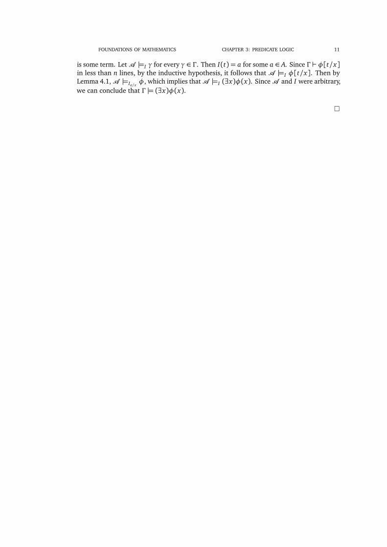
FOUNDATIONS OF MATHEMATICS CHAPTER 3: PREDICATE LOGIC 11
is some term. LetA |=I � for every � 2 � . Then I(t) = a for some a 2 A. Since � ` �[t/x]in less than n lines, by the inductive hypothesis, it follows that A |=I �[t/x]. Then byLemma 4.1,A |=Ia/x
�, which implies thatA |=I (9x)�(x). SinceA and I were arbitrary,we can conclude that � |= (9x)�(x).
⇤
FOUNDATIONS OF MATHEMATICSCHAPTER 4: MODELS FOR PREDICATE LOGIC
In this chapter, we will prove the completeness theorem for predicate logic by showing how tobuild a model for a consistent first-order theory. We will also discuss several consequences of thecompactness theorem for first-order logic and consider several relations that hold between variousmodels of a given first-order theory, namely isomorphism and elementary equivalence.
1. THE COMPLETENESS THEOREM FOR PREDICATE LOGIC
Fix a first-order theory L . For convenience, we will assume that our L -formulas are built uponly using ¬,_, and 9. We will also make use of the following key facts (the proofs of which wewill omit):
(1) If A is a tautology in propositional logic, then if we replace each instance of each proposi-tional variable in A with anL -formula, the resultingL -formula is true in allL -structures.
(2) For any L -structure A and any interpretation I into A,
A |=I (8x)�, A |=I ¬(9x)(¬�).We will also use the following analogues of results we proved in Chapter 2, the proofs of which
are the same:
Lemma 1.1. Let � be an L -theory.(1) If � is not consistent, then � ` � for every L -sentence �.(2) For an L -sentence �, � ` � if and only if � [ {¬�} is inconsistent.(3) If � is consistent, then for any L -sentence �, either � [ {�} is consistent or � [ {¬�} is
consistent.
The following result, known as the Constants Theorem, plays an important role in the proof ofthe completeness theorem.
Theorem 1.2 (Constants Theorem). Let � be an L -theory. If � ` �(c) and c does not appear in � ,then � ` (8x)�(x).
Proof. Given a proof of �(c) from � , let v be a variable not appearing in � . If we replace everyinstance of c with v in the proof of �(c), we have a proof of �(v) from � . Then by 8-Introduction,we have � ` (8x)�(x). ⇤
Gödel’s completeness theorem can be articulated in two ways, which we will prove are equiva-lent:
Theorem 1.3 (Completeness theorem, Version 1). For any L -theory � and any L -sentence �,
� |= �) � ` �.
Theorem 1.4 (Completeness theorem, Version 2). Every consistent theory has a model.
We claim that the two versions are equivalent.1

2 FOUNDATIONS OF MATHEMATICS CHAPTER 4: MODELS FOR PREDICATE LOGIC
Proof of claim. First, suppose that every consistent theory has a model, and suppose further that� |= �. If � is not consistent, then � proves every sentence, and hence � ` �. If, however, � isconsistent, we have two cases to consider. If � [ {¬�} is inconsistent, then by Lemma 1.1(2), itfollows that � ` �. In the case that �[{¬�} is consistent, by the second version of the completenesstheorem, there is some L -structure A such that A |= � [ {¬�}, from which it follows that A |= �and A |= ¬�. But we have assumed that � |= �, and hence A |= �, which is impossible. Thus, if �is consistent, it follows that � [ {¬�} is inconsistent.
For the other direction, suppose the first version of the completeness theorem holds and let� be an arbitrary L -theory. Suppose � has no model. Then vacuously, � |= ¬(� _ ¬�), where� is the sentence (8x)x = x . It follows from the first version of the completeness theorem that� ` ¬(� _¬�), and hence � is inconsistent. ⇤
We now turn to the proof of the second version of completeness theorem. As in the proof of thecompleteness theorem for propositional logic, we will use the compactness theorem, which comesin several forms (just as it did in with propositional logic).
Theorem 1.5. Let � be an L -theory.(1) For an L -sentence �, if � ` �, there is some finite �0 ✓ � , �0 ` �.(2) If every finite �0 ✓ � is consistent, then � is consistent.(3) If � = [n�n is , �n ✓ �n+1 for every n, and each �n is consistent, then � is consistent.
As in the case of propositional logic, (1) follows by induction on proof length, while (2) followsdirectly from (1) and (3) follows directly from (2).
Our strategy for proving the completeness theorem is as follows. Given � , we want to extend itto a maximally consistent collection of L -formulas, like the proof of the completeness theorem forpropositional logic. The problem that we now encounter (that did not occur in the propositionalcase) is that it is unclear how to make sentences of the form (9x)✓ .
The solution to this problem, due to Henkin, is to extend the language L to a language L 0 byadding new constants c0, c1, c2, . . . , which we will use to witness the truth of existential sentences.
Hereafter, let us assume that L is countably infinite (which is not a necessary restriction), sothat we will only need to add countably many new constants to our language. Using these constants,we will build a model of � , where the universe of our model consists of certain equivalence classeson the set of all L 0-terms with no variables (the so-called Herbrand universe of L 0). The modelwill satisfy a collection � ◆ � that is maximally consistent and Henkin complete, which means thatfor each L 0-formula ✓ (v) with exactly one free variable v, if (9v)✓ (v) is in �, then there is someconstant c in our language such that ✓ (c) is in �.
Proof of Theorem 1.4. Let �0,�1, . . . be an enumeration of allL 0-sentences. We define a sequence� =��1 ✓�0 ✓�1 ✓ . . . such that for each n 2 N,
�2n =⇢�2n�1 [ {�n} if �2n�1 [ {�n} is consistent,�2n�1 [ {¬�n} otherwise
and
�2n+1 =⇢�2n [ {✓ (cm)} if �n is of the form (9v)✓ (v) and is in �2n,�2n otherwise
where cm is the first constant in our list of new constants that has not appeared in �2n. Then wedefine � = [n�n.
We now prove a series of claims.

FOUNDATIONS OF MATHEMATICS CHAPTER 4: MODELS FOR PREDICATE LOGIC 3
Claim 1: � is complete (that is, for every L 0-sentence �, either � 2� or ¬� 2�).
Proof of Claim 1: This follows immediately from the construction.
Claim 2: Each �k is consistent.
Proof of Claim 2: We prove this claim by induction. First, ��1 = � is consistent by assumption.Now suppose that �k is consistent. If k = 2n for some n, then clearly �k is consistent, since if�2n�1 [ {�n} is consistent, then we set �k = �2n�1 [ {�n}, and if not, then by Lemma 1.1(3),�2n�1 [ {¬�n} is consistent, and so we set �k =�2n�1 [ {¬�n}.
If k = 2n+1 for some n, then if �n is not of the form (9v)✓ (v) or if it is but it is not in�2n, then�2n+1 =�2n is consistent by induction. If �n is of the form (9v)✓ (v) and is in �2n, then let c = cmbe the first constant not appearing in �2n. Suppose that �k =�2k+1 =�2n [ {✓ (c)} is not consis-tent. Then by Lemma 1.1(2), �2n ` ¬✓ (c). Then by the Constants Theorem, �2n ` (8x)¬✓ (x).But since �n is the formula (9v)✓ (v) and is in�2n, it follows that�2n is inconsistent, contradictingour inductive hypothesis. Thus �k =�2n+1 is consistent.
Claim 3: � = [n�n is consistent.
Proof of Claim 3: This follows from the third version of the compactness theorem.
Claim 4: � is Henkin complete (that is, for each L 0-formula ✓ (v) with exactly one free variableand (9v)✓ (v) 2�, then ✓ (c) 2� for some constant c).
Proof of Claim 4: Suppose that (9v)✓ (v) 2 �. Then there is some n such that (9v)✓ (v) is theformula �n. Since �2n�1 [ {�n} ✓ � is consistent, (9v)✓ (v) 2 �2n. Then by construction,✓ (c) 2�2n+1 for some constant c.
Our final task is to build a model A such that A |= �, from which it will follow that A |= �(since � ✓�). We define an equivalence relation on the Herbrand universe of L 0 (i.e., the set ofconstant L 0-terms, or equivalently, the L 0-terms that contain no variables). For constant terms sand t, we define
s ⇠ t, s = t 2�.
Claim 5: ⇠ is an equivalence relation.
Proof of Claim 5:
— Every sentence of the form t = t must be in � since � is complete, so ⇠ is reflexive.— If s = t 2�, then t = s must also be in � since � is complete, so ⇠ is symmetric.— If r = s, s = t 2�, then r = t must also be in � since � is complete, so ⇠ is transitive.
For a constant term s, let [s] denote the equivalence class of s. Then we define an L 0-structureas follows:
(i) A= {[t] : t is a constant term of L 0};(ii) for each function symbol f of the language L , we define
f A([t1], . . . , [tn]) = [ f (t1, . . . , tn)],
4 FOUNDATIONS OF MATHEMATICS CHAPTER 4: MODELS FOR PREDICATE LOGIC
where n is the arity of f ;(iii) for each predicate symbol P of the language L , we define
PA([t1], . . . , [tn]) if and only if P(t1, . . . , tn) 2�,
where n is the arity of P; and(iv) for each constant symbol c of the language L 0, we define
cA = [c].
Claim 6: A= (A, f , . . . , P, . . . , c, . . . ) is well-defined.
Proof of Claim 6: We have to show in particular that the interpretation of function symbols andpredicate symbols in A is well-defined. Suppose that s1 = t1, . . . , sn = tn 2� and
f A([t1], . . . , [tn]) = [ f (t1, . . . , tn)]. (1)
By our first assumption, it follows that � ` si = ti for i = 1, . . . , n. Then by term substitution,� ` f (s1, . . . , sn) = f (t1, . . . , tn), and so f (s1, . . . , sn) = f (t1, . . . , tn) 2�. It follows that
[ f (s1, . . . , sn)].= [ f (t1, . . . , tn)]. (2)
Combining (1) and (2) yields
f A([t1], . . . , [tn]) = [ f (t1, . . . , tn)] = [ f (s1, . . . , sn)] = f A([s1], . . . , [sn]).
A similar argument shows that the interpretation of predicate symbols is well-defined.
Claim 7: Let I be an interpretation into A. Then I(t) = [t] for every constant term t.
Proof of Claim 7: We verify this inductively for constant symbols and then for function symbolsapplied to constant terms.
— Suppose t is a constant symbol c. Then I(c) = cA = [c].— Suppose that t is the term f (t1, . . . , tn) for constant symbol f and constant terms t1, . . . , tn,
where I(ti) = [ti] for i = 1, . . . , n. Then
I( f (t1, . . . , tn)) = f A(I(t1), . . . , I(tn)) = f A([t1], . . . , [tn]) = [ f (t1, . . . , tn))].
Claim 8: A |= �. We verify this by proving that for every interpretation I into A and everyL 0-sentence �, A |=I � if and only if � 2�.
— If � is s = t for some terms s, t, then
A |=I s = t, I(s) = I(t), [s] = [t], s ⇠ t
, s = t 2�.
— If � is P(t1, . . . , tn) for some predicate symbol P, then
A |=I P(t1, . . . , tn), PA(I(t1), . . . , I(tn))
, PA([t1], . . . , [tn]), P(t1, . . . , tn) 2�.

FOUNDATIONS OF MATHEMATICS CHAPTER 4: MODELS FOR PREDICATE LOGIC 5
— If � is ¬ for some L 0-sentence , then
A |=I ¬ , A 6|= , /2�, ¬ 2�.
— If � is _ ✓ for some L 0-sentences and ✓ , then
A |=I _ ✓, A |= or A |= ✓, 2� or ✓ 2�, _ ✓ 2�.
— If � is (9v)✓ (v) for some L 0-formula ✓ with one free variable v, then
A |=I (9v)✓ (v), A |=Ib/v✓ (v) for some b 2 A
, A |=I ✓ (c) where b = [c], ✓ (c) 2�, (9v)✓ (v) 2�.
Since A |=�, it follows that A |= � . Note that A is an L 0-structure while � is only an L -theory(as it does not contain any expression involving any of the additional constants). Then let A⇤ bethe L -structure with the same universe as A and the same interpretations of the function symbolsand predicate symbols, but without interpreting the constants symbols that are in L 0 �L (theso-called reduct of A). Then clearly A⇤ |= � , and the proof is complete.
⇤
2. CONSEQUENCES OF THE COMPLETENESS THEOREM
The same consequences we derived from the Soundness and Completeness Theorem for Propo-sitional Logic apply now to Predicate Logic with basically the same proofs.
Theorem 2.1. For any set of sentences � , � is satisfiable if and only if � is consistent.
Theorem 2.2. If ⌃ is a consistent theory, then ⌃ is included in some complete, consistent theory.
We also have an additional version of the compactness theorem, which is the most commonformulation of compactness.
Theorem 2.3 (Compactness Theorem for Predicate Logic).An L -theory � is satisfiable if and only if every finite subset of � is satisfiable.
Proof. ()) If A |= � , then it immediately follows that A |= �0 for any finite �0 ✓ � .
(() Suppose that � is not satisfiable. By the completeness theorem, � is not consistent. Then� ` � & ¬� for some L -sentence �. Then by the first formulation of the compactness theoremthere is some finite �0 ✓ � such that �0 ` � & ¬�. It follows that �0 is not satisfiable. ⇤
We now consider two applications of the compactness theorem, the first yielding a model ofarithmetic with infinite natural numbers and the second yielding a model of the real numbers withinfinitesimals.

6 FOUNDATIONS OF MATHEMATICS CHAPTER 4: MODELS FOR PREDICATE LOGIC
Example 2.4. Let L = {+,⇥,<, 0, 1} be the language of arithmetic, and let � = Th(N), the setof L -sentences true in the standard model of arithmetic. Let us expand L to L 0 by adding a newconstant c to our language. We extend � to an L 0-theory � 0 by adding all sentences of the form
n : c > 1+ . . .+ 1| {z }n times
We claim that every finite � 00 ✓ � 0 is satisfiable. Given any finite � 00 ✓ � 0, � 00 consists of at most finitelymany sentences from � and at most finitely many sentences of the form i . It follows that
� 00 ✓ � [ { n1, n2
, . . . , nk}
for some n1, n2, . . . , nk 2 N, where these latter sentences assert that c is larger than each of the valuesn1, n2, . . . , nk. Let n = max{n1, . . . , nk} then let A = (N,+,⇥,<, 0, 1, n), so that cA = n and henceA |= � 00. Then by the compactness theorem, there is some L 0-structure B such that B |= � 0. In theuniverse of B, we have objects that behave exactly like 0, 1, 2, 3, . . . (in a sense we will make preciseshortly), but the interpretation of c in B satisfies cB > n for every n 2 N and hence behaves like aninfinite natural number. We will write the universe of B as N⇤.Example 2.5. Let L consist of
— an n-ary function symbol Ff for every f : Rn! R;— an n-ary predicate symbol PA for every A✓ Rn; and— a constant symbol cr for every r 2 R.
Let R be the L -structure with universe R satisfying— FR
f = f for every function symbol Ff ;
— PRA = A for every predicate symbol PA; and
— cRr = r for every constant symbol cr .Let us expand L to L 0 by adding a new constant d to our language. We extend � to an L 0-theory � 0
by adding all sentences of the form✓r : c0 < d < cr
for r 2 R>0. As in the previous example, every finite � 00 ✓ � 0 is satisfiable. Hence by the compactnesstheorem, � 0 is satisfiable. Let A |= � . The universe of A contains a copy of R (in a sense we will makeprecise shortly). In addition, dA is infinitesimal object. For every real number in A, 0< dA < r holds.We will write the universe of A as R⇤.
Now we consider a question that was not appropriate to consider in the context of propositionallogic, namely, what are the sizes of models of a given theory? Our main theorem is a consequenceof the proof of the Completeness Theorem. We proved the Completeness Theorem only in the caseof a countable language L, and we built a countable model (which was possibly finite). By using alittle care (and some set theory), one can modify steps (1) and (2) for an uncountable language todefine by transfinite recursion a theory � and prove by transfinite induction that � has the desiredproperties. The construction leads to a model whose size is at most the size of the language withwhich one started. Thus we have:
Theorem 2.6 (Löwenheim-Skolem Theorem). If � is an L -theory with an infinite model, then �has a model of size for every infinite with |L | .
Proof Sketch. First we add new constant symbols hd↵ | ↵ < i to our language L . Next weexpand � to � 0 by adding formulas that say d↵ 6= d� for the different constants:
� 0 = � [�¬d↵ = d� : ↵< � <
.

FOUNDATIONS OF MATHEMATICS CHAPTER 4: MODELS FOR PREDICATE LOGIC 7
Since � has an infinite model, each finite � 00 ✓ � 0 has a model. Hence by the compactnesstheorem, � 0 has a model. By the soundness theorem, � 0 is consistent. Then use the proof of thecompleteness theorem to define a model B0 of � 0 the universe of which has size |B| . SinceB0 |= d↵ 6= d� for ↵ 6= � , there are at least many elements. Thus |B|= and so � 0 has a modelB0 of the desired cardinality. Let B be the reduct of B0 obtained by removing the new constantsymbols from our expanded language. Then B is a model of the desired size for � . ⇤
3. ISOMORPHISM AND ELEMENTARY EQUIVALENCE
We conclude this chapter with a discussion of isomorphic models and the notion of elementaryequivalence.
Definition 3.1. Given L -structures A and B, a bijection H : A!B is an isomorphism if it satisfies:(1) For every constant c 2 L , H(cA) = cB.(2) For every k-ary predicate symbol P 2 L and every a1, . . . , ak 2 A,
PA(a1, . . . , ak), PB(H(a1), . . . , H(ak)).
(3) For every k-ary function symbol F 2 L and every a1, . . . , ak 2 A,
H(FA(a1, . . . , ak)) = FB(H(a1), . . . , H(ak)).
Furthermore, A and B are isomorphic, denoted A⇠=B, if there exists an isomorphism between A andB.
Example 3.2. The ordered group (R,+,<) of real numbers under addition is isomorphic to theordered group (R>0, ·,<) of positive real numbers under multiplication under the mapping H(x) = 2x .The key observation here is that H(x + y) = 2x+y = 2x · 2y = H(x) ·H(y).
We compare the relation of isomorphism with the following relation between models.
Definition 3.3. L -structures A and B are elementarily equivalent, denoted A ⌘ B, if for anyL -sentence �,
A |= �,B |= �.
How do the relations of ⇠= and ⌘ compare? First, we have the following theorem.
Theorem 3.4. If A and B are L -structures satisfying A⇠=B, then A⌘B.
The proof is by induction on the complexity of L -sentences. The converse of this theorem doesnot hold, as shown by the following example.
Example 3.5. (Q,) and (R,), both models of the theory of dense linear orders without endpoints,are elementarily equivalent, which follows from the fact that the theory of dense linear orders withoutendpoints is complete (which we will prove in Chapter 6). Note, however, that these structures are notisomorphic, since they have different cardinalities.
We conclude this chapter with one last set of definitions and examples.
Definition 3.6. Let A and B be L -structures with corresponding domains A✓ B.(1) A is a submodel of B (A ✓B) if the following are satisfied:
(a) for each constant c 2 L , cA = cB;(b) for each n-ary function symbol f 2 L and each a1, . . . , an 2 A,
f A(a1, . . . , an) = f B(a1, . . . , an);

8 FOUNDATIONS OF MATHEMATICS CHAPTER 4: MODELS FOR PREDICATE LOGIC
(c) for each n-ary relation symbol R 2 L and each a1, . . . , an 2 A,
RA(a1, . . . , an), RB(a1, . . . , an).
(2) A is an elementary submodel of B (written A≠B) if(a) A is a submodel of B;(b) for each L -formula �(x1, . . . , xn) and each a1, . . . , an 2 A,
A |= �(a1, . . . , an),B |= �(a1, . . . , an).
Example 3.7. Consider the rings (Z, 0, 1,+, ·) ✓ (Q, 0, 1,+, ·) ✓ (R, 0, 1,+, ·).— (Z, 0, 1,+, ·) is a submodel of (Q, 0, 1,+, ·) and (Q, 0, 1,+, ·) is a submodel of (R, 0, 1,+, ·).— (Z, 0, 1,+, ·) is not an elementary submodel of (Q, 0, 1,+, ·), since Q |= (9x)x + x = 1 which
is false in Z.— Neither (Z, 0, 1,+, ·) nor (Q, 0, 1,+, ·) is an elementary submodel of (R, 0, 1,+, ·) since R |=(9x)x · x = 2, which is false in both Z and Q.
Example 3.8. The following elementary submodel relations hold:— (Q,)≠ (R,)— (N, 0, 1,+, ·)≠ (N⇤, 0, 1,+, ·).— (R, 0, 1,+, ·)≠ (R⇤, 0, 1,+, ·).
The latter two items in the previous example justify the claims that the natural numbers arecontained in models of non-standard arithmetic and that the real numbers are contained in modelsof non-standard analysis.
We conclude with one last example.
Example 3.9. Z3 = {0, 1, 2} with addition modulo 3 is not a submodel of Z6 = {0, 1, 2, 3, 4, 5} withaddition modulo 6 because they have different addition functions: In Z3, 2+ 2 = 1 whereas in Z6,2+ 2= 4. However, Z3 is isomorphic to the subgroup of Z6 consisting of {0, 2,4}.

FOUNDATIONS OF MATHEMATICSCHAPTER 5: COMPUTABILITY THEORY
1. INTRODUCTION AND EXAMPLES
There are many different approaches to defining the collection of computable number-theoreticfunctions. The intuitive idea is that a function F : N ! N (or more generally F : Nk ! N) iscomputable if there is an algorithm or effective procedure for determining the output F(m) fromthe input m. To demonstrate that a particular function F is computable, it suffices to give thecorresponding algorithm.
Example 1.1. Basic computable functions include(i) the successor function S(x) = x + 1,
(ii) the addition function +(x , y) = x + y , and(iii) the multiplication function ·(x , y) = x · y .
Example 1.2. Some slightly more complicated examples of computable functions:(i) The Division Algorithm demonstrates that the two functions that compute, for inputs a
and b, the unique quotient q = q(a, b) and remainder r = r(a, b), with 0 r < a, suchthat b = qa+ r, are both computable.
(ii) The Euclidean Algorithm demonstrates that the function gcd(a, b) which computes thegreatest common divisor of a and b is computable. It follows that least common multiplefunction lcm(a, b) = (a · b)/gcd(a, b) is also computable
The notion of computability for functions can be extended to subsets of N or relations on Nk
for some k as follows. First, a set A✓ N is said to be computable if the characteristic function of A,defined by
�A(n) =ß
1 if n 2 A0 if n /2 A,
is a computable function. Similarly, a relation R ✓ Nk is said to be computable if its characteristicfunction
�A(n1, . . . , nk) =ß
1 if (n1, . . . , nk) 2 R0 if (n1, . . . , nk) /2 R
is computable. These definitions are equivalent to saying that there is an algorithm for testingwhether a given number is in A or whether a given finite sequence (n1, . . . , nk) is in R.
Example 1.3. The following are computable:(i) The set of perfect squares is computable, since given a number n, we can test whether it is
a square by computing m2 for all m n and checking whether m2 = n.(ii) The relation x | y (“x divides y”) is computable, since by the Division Algorithm, x | y if
and only if the remainder r(x , y) = 0.(iii) The set of even numbers is computable, since n is even if and only if 2 | n.
1
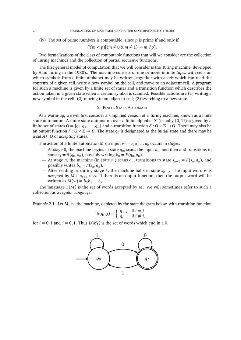
2 FOUNDATIONS OF MATHEMATICS CHAPTER 5: COMPUTABILITY THEORY
(iv) The set of prime numbers is computable, since p is prime if and only if
(8m< p)[(m 6= 0 & m 6= 1)! m 6 | p].Two formalizations of the class of computable functions that will we consider are the collection
of Turing machines and the collection of partial recursive functions.
The first general model of computation that we will consider is the Turing machine, developedby Alan Turing in the 1930’s. The machine consists of one or more infinite tapes with cells onwhich symbols from a finite alphabet may be written, together with heads which can read thecontents of a given cell, write a new symbol on the cell, and move to an adjacent cell. A programfor such a machine is given by a finite set of states and a transition function which describes theaction taken in a given state when a certain symbol is scanned. Possible actions are (1) writing anew symbol in the cell; (2) moving to an adjacent cell; (3) switching to a new state.
2. FINITE STATE AUTOMATA
As a warm-up, we will first consider a simplified version of a Turing machine, known as a finitestate automaton. A finite state automaton over a finite alphabet ⌃ (usually {0,1}) is given by afinite set of states Q = {q0, q1, . . . , qk} and a transition function � : Q⇥⌃!Q. There may also bean output function F : Q⇥⌃! ⌃. The state q0 is designated as the initial state and there may bea set A✓Q of accepting states.
The action of a finite automaton M on input w= a0a1 . . . ak occurs in stages.— At stage 0, the machine begins in state q0, scans the input a0, and then and transitions to
state s1 = �(q0, a0), possibly writing b0 = F(q0, a0).— At stage n, the machine (in state sn) scans an, transitions to state sn+1 = F(sn, an), and
possibly writes bn = F(sn, an).— After reading ak during stage k, the machine halts in state sk+1. The input word w is
accepted by M if sk+1 2 A. If there is an ouput function, then the output word will bewritten as M(w) = b0 b1 . . . bk.
The language L(M) is the set of words accepted by M . We will sometimes refer to such acollection as a regular language.
Example 2.1. Let M1 be the machine, depicted by the state diagram below, with transition function
�(qi , j) =ß
q1�i if i = jqi if i 6= j,
for i = 0,1 and j = 0,1. Thus L(M1) is the set of words which end in a 0.
q0 q1
q0 q1
0
0
11
0
1
01

FOUNDATIONS OF MATHEMATICS CHAPTER 5: COMPUTABILITY THEORY 3
Example 2.2. Let M2 be the machine, depicted by the state diagram below, with transition function
�(qi , j) =ß
q1�i if j = 0qi if j = 1,
for i = 0,1. Thus L(M2) is the set of words which contain an even number of 0’s.
q0 q1
q0 q1
0
0
11
0
1
01Next we consider some finite state automata which compute functions. We want to express
natural numbers in reverse binary notation, so that the word a0a1 . . . ak represents a0 + 2a1 + · · ·+2kak.
Example 2.3. The successor machine M3 computes S(x) = x + 1. State q0 is the carry state andstate q1 is the no-carry state. The edges in the state diagram below are labelled with symbols ofthe form i : j, which means that i is an input bit and j is an output bit.
For reasons that will be clear shortly, we require that any number of the form 2n � 1 (normallyrepresented by a string of the form 1n) to be represented by 1n0. For any other number, addingadditional zeros to the end of its representation will make no difference.
Starting in state q0, the machine outputs (i + 1) mod 2 on input i and transitions to state q1�i .From state q1 on input i, the machine outputs i and remains in state q1. We take the liberty ofadding an extra 0 at the end of the input in order to accommodate the carry.
q0 q1
0:1
0:0, 1:11:0
More precisely, the transition function and output function of M3 are defined by
�(qi , j) =ß
q0 if i = 0 & j = 1q1 if (i = 0 & j = 0)_ i = 1
and
F(qi , j) =ß
1� j if i = 0j if i = 1 .
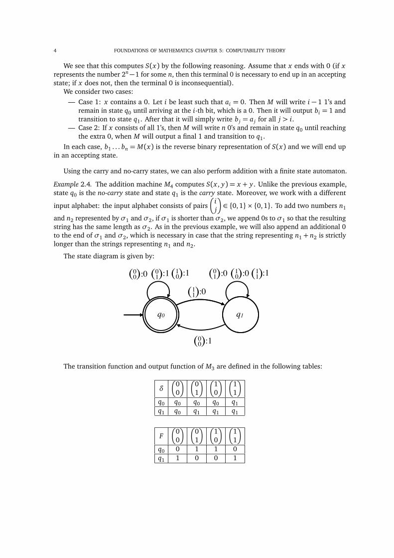
4 FOUNDATIONS OF MATHEMATICS CHAPTER 5: COMPUTABILITY THEORY
We see that this computes S(x) by the following reasoning. Assume that x ends with 0 (if xrepresents the number 2n�1 for some n, then this terminal 0 is necessary to end up in an acceptingstate; if x does not, then the terminal 0 is inconsequential).
We consider two cases:— Case 1: x contains a 0. Let i be least such that ai = 0. Then M will write i � 1 1’s and
remain in state q0 until arriving at the i-th bit, which is a 0. Then it will output bi = 1 andtransition to state q1. After that it will simply write bj = aj for all j > i.
— Case 2: If x consists of all 1’s, then M will write n 0’s and remain in state q0 until reachingthe extra 0, when M will output a final 1 and transition to q1.
In each case, b1 . . . bn = M(x) is the reverse binary representation of S(x) and we will end upin an accepting state.
Using the carry and no-carry states, we can also perform addition with a finite state automaton.
Example 2.4. The addition machine M4 computes S(x , y) = x + y . Unlike the previous example,state q0 is the no-carry state and state q1 is the carry state. Moreover, we work with a different
input alphabet: the input alphabet consists of pairsÅ
ij
ã2 {0, 1}⇥ {0, 1}. To add two numbers n1
and n2 represented by �1 and �2, if �1 is shorter than �2, we append 0s to �1 so that the resultingstring has the same length as �2. As in the previous example, we will also append an additional 0to the end of �1 and �2, which is necessary in case that the string representing n1 + n2 is strictlylonger than the strings representing n1 and n2.
The state diagram is given by:
q0 q1
:0( )00
( )00 :1
( )01 :0( )0
1 :1 ( )10 :0( )1
0 :1
( )11 :0
( )11 :1
The transition function and output function of M3 are defined in the following tables:
�
Å00
ã Å01
ã Å10
ã Å11
ã
q0 q0 q0 q0 q1q1 q0 q1 q1 q1
FÅ
00
ã Å01
ã Å10
ã Å11
ã
q0 0 1 1 0q1 1 0 0 1

FOUNDATIONS OF MATHEMATICS CHAPTER 5: COMPUTABILITY THEORY 5
For any finite state automaton M , the set L(M) of words accepted by M is a computable set.Moreover, if M computes a function f , then f is also computable. However, many computablesets and functions cannot be computed by a finite automaton.
Example 2.5. The function f (x) = x2 is not computable by a finite state automaton. Supposethat M computes x2 on input x , where we have appended a sufficient number of 0’s to the end ofthe input so that we can output x2 (recall that each input bit yields at most one output bit). Inparticular, for any n, M will output 02n1 on input 0n1, since f (2n) = (2n)2 = 22n. Thus, on input0n1, after reading the first n+ 1 bits, M needs to examine at least n additional 0’s and write atleast n additional 0’s before it finishes the output with a final 1. Now suppose that M has k statesand let n> k+ 1. Let s j be the state of the machine after reading 0n10 j . Then there must be somei, j k+1< n such that si = s j . Furthermore, every time M transitions from state si upon readinga 0, M must output a 0. But the machine is essentially stuck in a loop and hence can only printanother 0 after reading 0n10n when it needs to print the final 1.
3. TURING MACHINES
A Turing machine is a simple model of a computer that is capable of computing any functionthat can be computed. It consists of these items:
(1) a finite state control component with a finite number of read/write heads; and(2) a finite number of unbounded memory tapes (one or more for the input(s), one for
the output, and the rest for scratchwork), each of which is divided into infinitely manyconsecutive squares in which symbols can be written.
Furthermore, it must satisfy these conditions:(1) there is a specified initial state q0 and a specified final qH , or halting, state; and(2) each read/write head reads one cell of each tape and either moves one cell to the left (L),
moves one cell to the right (R), or stays stationary (S) at each stage of a computation.The notion of Turing machine is formalized in the following definition.
Definition 3.1. A k-tape Turing machine M for an alphabet ⌃ consists of(i) a finite set Q = {q0, . . . , qn} of states;
(ii) an alphabet ⌃;(iii) a transition function � : Q⇥⌃k! ⌃k ⇥ {L,R,S}k;(iv) q0 2Q is the start state; and(v) qH 2Q is the halting or final state.
A move of M in a given state qi, scanning the symbols a1, . . . , ak on the k tapes, where�(qi , a1, . . . , ak) = (qj , b1, . . . , bk, D1, . . . , Dk), consists of the following actions:
(1) switching from state qi to state qj;(2) writing bi (and thus erasing ai) on tape i; and(3) moving the head on tape i in the direction Di .
A computation always begins with(i) the machine in state q0;
(ii) some finite input on each of the input tapes; and(iii) each of the input heads scanning the first symbol on each of the input tapes.
The configuration of a machine at a given stage of a computation consists of(i) the current state of the machine;

6 FOUNDATIONS OF MATHEMATICS CHAPTER 5: COMPUTABILITY THEORY
(ii) the contents of each tape; and(iii) the location of each of the heads on each tape.
M machine halts after n moves if it transitions to the halting state in the n-th stage of the computa-tion. A machine M accepts a word w, denoted M(w)#, if the machine halts (i.e. ends up in thehalting state) when given the input w. In this case, we say M halts on the input w. Otherwise, wesay that M diverges on input w, denoted M(w)".
It is an essential feature of Turing machines that they may fail to halt on some inputs. This givesrise to the partial computable function fM which has domain {w : M(w) #}. That is, fM (w) = y ifand only if M halts on input w and y appears on the output tape when M halts, meaning that theoutput tape contains y surrounded by blanks on both sides. (For the sake of elegance, we mayinsist that the first symbol of y is scanned at the moment of halting.) Sometimes we will write thevalue fM (w) as M(w).
Example 3.2. We define a Turing machine M1 that computes x + y . There are two input tapes andone output tape. The numbers x and y are written on separate input tapes in reverse binary form.M has the states: the initial state q0, a carry state q1 and the halting state qH . The two input tapesare read simultaneously in the form a/b. We need to consider blanks squares as symbols # in caseone input is longer and/or there is a carry at the end. The behavior of M1 is summed up in thefollowing table.
State Read Write Move New Stateq0 0/0 0 R q0q0 0/# 0 R q0q0 #/0 0 R q0q0 0/1 1 R q0q0 1/0 1 R q0q0 1/# 1 R q0q0 #/1 1 R q0q0 1/1 0 R q1q0 #/# # S qHq1 0/0 1 R q0q1 0/# 1 R q0q1 #/0 1 R q0q1 0/1 0 R q1q1 1/0 0 R q1q1 1/# 0 R q1q1 #/1 0 R q1q1 1/1 1 R q1q1 #/# 1 S qH
Example 3.3. We roughly describe a Turing machine M2 that computes x · y. Again there aretwo input tapes and one output tape. The idea is that if y =
Pi2I 2i for some finite I ✓ N, then
x · y =P
i2I 2i · x . For each i, 2i · x has the form of i 0’s followed by x . For example, if x = 1011(thirteen), then 4 · x = 001011 (fifty-two).

FOUNDATIONS OF MATHEMATICS CHAPTER 5: COMPUTABILITY THEORY 7
To multiply 1011 by 100101 we add
20 · 13+ 23 · 13+ 25 · 13= 1011+ 0001011+ 000001011.
We begin in state q0 with x and y each written on one of the input tapes (tapes 1 and 2) inreverse binary notation, and all three reader heads lined up. We first add a terminal 0 to the endof y , which is necessary to ensure that our computation will halt.
Suppose there are k initial 0’s in y . For each such 0, we replace it with a #, write a 0 on tape 3in the corresponding cell, move the heads above tapes 2 and 3 one cell to the right, and stay instate q0.
When we encounter the first 1 of y , we replace this 1 with a # and transition to a state qC inwhich we copy x to tape 3 (the output tape), beginning in the i-th cell of this tape. As the contentsof tape 1 are being copied onto tape 3, we also require that head above tape 2 moves in the samedirections as the head above tapes one and three until we encounter the first # on tape one. (Onecan verify that the heads above tapes 2 and 3 will always be lined up). We then transition to astate in which we reset the position of the tape 1 head to scanning the first bit of x , and then thetape 2 head is scanning the leftmost bit in y that has not been erased (i.e. replaced with a #). Asabove, we require that the tape 3 head moves in the same directions as the tape 2 head during thisphase (which will ensure that we begin copying x in the correct place on the tape if the next bit ofy happens to be a 1. We then transition back to state q0 and continue as before.
Suppose that the next bit of y that is equal to 1 is the i-th bit of y . Then we start the additionby adding the first bit of x to the i-th bit of the output tape. We note that we may need to utilize acarry state during the addition. When we reach the # at the end of y , the computation is complete,and we transition to the halting state. For an example of the product 7 . . . 8= 7 · 8= 56, see thesupplementary document TuringMachineMultiplication.pdf.
Like finite state automata, Turing machines can be represented a state diagram.
Example 3.4. There is a Turing machine that accepts every string in the set {an bncn | n> 0} overthe alphabet ⌃ = {a, b, c, 0, #}.
Here we will use the “0” as a special marking symbol, although we can do without it (and use“a” instead). The following state diagram gives a Turing machine which accepts this every string inthe above set.

8 FOUNDATIONS OF MATHEMATICS CHAPTER 5: COMPUTABILITY THEORY
q0 q1
……
……
a a a a b b b b c c c c
q2q3
a,# a,R#,R
a,# a,R
# # # # # # # # # # # # # # # #
# # # #
0,R
1
2
b,# b,R#,L
b,0 b,R0,L
c,# c,Rc,0 c,R
0,R
#,# #,S#,SqH
#,R
q4
Observe that q4 functions as a reject state. Any input not listed on any of the edges will cause atransition to state q4. To see that this Turing machine accepts the desired set, see the supplementarydocument Turingmachine-a4b4c4.pdf for an example with input aaaabbbbcccc.
Example 3.5. We define a Turing machine M that computes the function f (x) = |x | (the length ofa string x). There are two tapes, the input tape and the output tape. The input tape is read-onlybut we allow writing on the output tape. Let the input alphabet be ⌃ = {a}. Let ↵/� indicate thatthe machine is currently reading ↵ on the input tape and � on the output tape. Similarly D1/D2indicates that the head on the input tape moves in direction D1 while the head on the output tapemoves in direction D2. The idea is to add one to the output tape after reading each symbol of theinput tape. State q1 arises when we need to add one to the output by carrying. State q2 simplybrings the output tape back to the first bit. Certain transitions are omitted from the table sincethey lead to divergent computation (we will assume that incorrect inputs will immediately causea transition to a reject state). For example, we only get to state q1 when we have read a on thefirst tape and we continute to read that a, so that the input #/0 is not a legal input when we havereached state q1.
The following table describes the behavior of the three main states.

FOUNDATIONS OF MATHEMATICS CHAPTER 5: COMPUTABILITY THEORY 9
state read write move new stateq0 a/# a/1 R/S q0q0 a/0 a/1 R/S q0q0 a/1 a/0 S/R q1q0 #/0 #/0 S/S qHq0 #/1 #/0 S/S qHq0 #/# #/0 S/S qHq1 a/# a/1 S/L q2q1 a/0 a/1 S/L q2q1 a/1 a/0 S/R q1q2 a/# a/# R/R q0q2 a/0 a/0 S/L q2q2 a/1 a/1 S/L q2
We now prove some general facts about certain kinds of languages that are central to the studyof Turing machines.
For a fixed alphabet ⌃, a language is simply a set L ✓ ⌃⇤ (recall that ⌃⇤ is the collection of allfinite sequences of elements of ⌃).
Definition 3.6. A language L is said to be Turing semicomputable if there is a Turing machine Msuch that L = {w : M(w)#}. L is a Turing computable language if the characteristic function of L isTuring computable.
Example 3.7. Here is a simple Turing machine M such that M(w)# if and only if w contains a 0. Instate q0, M moves right and remains in state q0 upon reading a 1 or a blank. M immediately haltsupon reading a 0.
Proposition 3.8. Every Turing computable language is also Turing semicomputable.
Proof. Let M be a Turing machine that computes the characteristic function of L. We modify M todefine a machine M 0 as follows. First we introduce new states qA and qB. Replace any transitionthat goes to the halting state qH with a transition that goes the the state qA. For the qA state, addtwo transitions. If the output tape reads 1, then transition to the halting state qH . If the outputtape reads 0, then move the output tape head one cell to the right and transition to state qB. Instate qB, move the output tape head one cell to the left and return to state qA. Then M 0(w) willhalt if and only if M(w) = 1 and will endlessly alternate between states qA and qB if and only ifM(w) = 0. ⇤Proposition 3.9. L is Turing computable if and only if both L and its complement are Turingsemicomputable.
Proof. First observe that if L ✓ ⌃⇤ is Turing computable, then ⌃⇤ � L is Turing computable. Indeed,if M computes the characteristic function of L, then define M 0 to be the machine that behavesexactly like M except that for i = 0, 1 whenever M writes i on its output tape, M 0 writes 1� i onits output tape. It follows from Proposition 3.8 that if L is Turing computable, then both L and itscomplement are semicomputable.
Now suppose that L = {w : M0(w)#} and that ⌃⇤ � L = {w : M1(w)#} for two Turing machinesM0 and M1. We define a Turing machine M such that the function fM computed by M is thecharacteristic function of L. Suppose for the sake of simplicity that M0 and M1 each have one
10 FOUNDATIONS OF MATHEMATICS CHAPTER 5: COMPUTABILITY THEORY
input tape and have no output tape. Then M will have one input tape, two scratch tapes, and oneoutput tape. The states of M will include pairs (q, q0) where q is a state of M0 and q0 is a state ofM1. Given w on the input tape of M , M will begin by copying w onto each of the scratch tapesand transitioning to the pair (q0, q00) of initial states of M0 and M1. On the first scratch tape, Mwill simulate M0, while on the second scratch tape, M will simulate M1. Eventually M will enter astate of one of the two forms: (qH , r), where qH is the halting state of M0 and r is a non-haltingstate of M1, or (q, q0H), where q0H is the halting state of M1 and q is a non-halting state of M0.
— If M enters a state of the form (qH , r), this means that the machine M0 has halted on w,and hence w 2 L. M will thus write a 1 on its output tape and transition to its haltingstate.
— If M enters a state of the form (q, q0H), this means that the machine M1 has halted on w,and hence w /2 L. M will thus write a 0 on its output tape and transition to its haltingstate.
Note that M will never enter the state (qH , q0H), since M0 and M1 can never accept the same word.It thus follows that M computes the characteristic function of L. ⇤
Given two Turing machines M0 and M1, we write M0(x)' M1(x) to mean that (i) M0(x)# ifand only if M1(x)# and (ii) M0(x)# implies that M0(x) = M1(x).
Theorem 3.10. Fix a finite alphabet ⌃ = {0,1, q,#,⇤, L, R, S, H,#}. There is a universal Turingmachine U : ⌃⇤ ⇥ ⌃⇤ ! ⌃⇤ such that, for any Turing machine M : {0,1}⇤ ! {0,1}⇤, there existswM 2 ⌃⇤ such that, for all inputs x 2 {0,1}⇤, U(wM , x)' M(x).
We will only sketch the main ideas in the proof of Theorem 3.10. To simplify matters, we willuse the following lemma.
Lemma 3.11. Let M be a k-tape Turing machine for some k > 1. Then there is a single-tape Turingmachine M 0 such that M(x)' M 0(x) for all x 2 ⌃⇤.Proof of Theorem 3.10. (Sketch) We define a universal Turing machine with two input tapes, ascratch tape, and an output tape. For each machine M , we would like to define a word wM 2 ⌃⇤that encodes all of the information of M . We will let wM be the entire transition table of M writtenas one long string in the alphabet ⌃⇤, with a ⇤ separating each entry on a given row of a table and⇤⇤ separating each row of the table. The string q0 will stand for the initial state, qH will stand forthe halting state, and all other states will be coded by a q followed by a finite string of 1s (q1, q11,q111, etc.)
Now, given the code wM for a machine M , to compute U(wM , x) (i.e. M(x)), U proceeds bywriting the initial configuration of M with input x on its scratch tape. Suppose, for example thatx = 000. Then U will write
q0⇤ # 000where the # specifies that the reader head is above the first 0 on the input tape of M . To proceed,U simply consults the transition table wM written on its first input tape and writes the resultingconfiguration of M after one move on its scratch tape. Continuing the example from above, if thefirst move of M is to change to state q1, replace the first 0 of x with a 1 and move the head onecell to the right, the resulting configuration will be
q1 ⇤ 1 # 00
Continuing in this way, if M(x)#, then U will eventually come to a stage in which a haltingconfiguration is written on its scratch tape. In this halting configuration, the value y = M(x) will

FOUNDATIONS OF MATHEMATICS CHAPTER 5: COMPUTABILITY THEORY 11
be written, and so U can simply copy this value y to its output tape and transition to its ownhalting state. Lastly, if M(x)", then U(wM , x)".
⇤It is important to note that our use of the alphabet ⌃ in the definition of a universal Turing
machine is not strictly necessary. For instance, we can also define a universal Turing machineU : {0, 1}⇤ ⇥ {0, 1}⇤ ! {0, 1}⇤ by representing each of the symbols in ⌃ as a unique binary string.Some caution is necessary to make sure the coding is unambiguous. We will not discuss the detailsof such a coding here, but we will assume that for each Turing machine M , there is some uniquewM 2 {0,1}⇤ that codes M . Moreover, we will assume that every x 2 {0,1}⇤ codes some Turingmachine, which we will write as Mx . (We will justify these assertions in Chapter 7 when we discussGödel numbering.)
Programs nearly always have bugs, so they may not do want we want them to do. The problemof determining whether a given Turing machine M halts on input string w is the Halting Problem.Let us define the halting set to be H = {(x , y) 2 {0,1} ⇤ ⇥{0,1}⇤ : Mx(y)#}. Observe that H issemicomputable: (x , y) 2 H if and only if U(x , y)#. By contrast, we have the following.
Theorem 3.12. The Halting Problem is not computable.
Proof. We will show that the complement of H is not semicomputable, so that by Proposition 3.9,H is not computable. Suppose by way of contradiction that there is a Turing machine M such that,for all x , y 2 {0, 1}⇤,
M(x , y)# () Mx(y)".We can define a Turing machine N so that N(w)' M(w, w). Then
N(w)# () Mw(w)".But this Turing machine N must have some code e. So for all w,
Me(w)# () Mw(w)".The contradiction arises when w= e. ⇤
Thus there exists a set which is semicomputable but not computable.
4. RECURSIVE FUNCTIONS
In this section, we define the primitive recursive and the (partial) recursive functions and showthat they are all Turing computable. Each function f maps from Nk to N for some fixed k (the arityof f ).
Definition 4.1. The collection of primitive recursive functions is the smallest collectionF of functionsfrom Nk to N for each k > 0 that includes the following initial functions
(1) the constant function c(x) = 0,(2) the successor function s(x) = x + 1,(3) the projection functions pk
i (x1, . . . , xk) = xk for each k 2 N and i = 1, . . . , k,and are closed under the following schemes for defining new functions:
(4) (composition) if f : Nk! N and gi : N j ! N for i = 1, . . . , k (where j, k > 0) are in F , thenthe function h : N j ! N defined by
h(x1, . . . , x j) = f (g1(x1, . . . , x j), . . . , gk(x1, . . . , x j))
is in F , and

12 FOUNDATIONS OF MATHEMATICS CHAPTER 5: COMPUTABILITY THEORY
(5) (primitive recursion) if g : Nk! N and h : Nk+2! N are inF , then the function f : Nk+1!N defined by
f (0, x1, . . . , xk) = g(x1, . . . , xk)f (n+ 1, x1, . . . , xk) = h(n, x1, . . . , xk, f (n, x1, . . . , xk))
is in F .
Example 4.2.
(1) For any constant c 2 N, the function h(x) = c is primitive recursive. The proof is byinduction on c. For c = 0, this follows from the fact that the initial function c(x) = 0is primitive recursive. Supposing that g(x) = c is primitive recursive and using thefact that s(x) = x + 1 is primitive recursive, we can use composition to conclude thath(x) = s(g(x)) = g(x) + 1= c + 1 is primitive recursive.
(2) For any k and any c, the constant function f : Nk! N with f (x1, . . . , xk) = c is primitiverecursive. We have h(x) = c by (1) and we have pk
1(x1, . . . , xk) = x1 as a basic function,so that f (x1, . . . , xk) = h(pk
1(x1, . . . , xk)) = h(x1) = c is also primitive recursive.
(3) The addition function f (x , y) = x + y is primitive recursive. Let g(y) = p11(y) and
h(x , y, z) = c(p33(x , y, z)). Then f is given by
f (0, y) = g(y) = y
f (n+ 1, y) = h(n, y, f (n, y)) = f (n, y) + 1.
(4) The predecessor function f (x) = x .� 1 =⇢
x � 1, if x > 00, if x = 0
is primitive recursive. Let
g(x) = c(x) and h(x , y) = p21(x , y). Then f is given by
f (0) = g(y) = 0
f (n+ 1) = h(n, f (n)) = n.
(5) The truncated subtraction function f (x , y) =⇢
y .� x , if x y0, otherwise
is primitive recursive.
Let g(y) = p11(y) and h(x , y, z) = z .� 1. Then f is given by
f (0, y) = g(y) = y
f (n+ 1, y) = h(n, y, f (n, y)) = f (n, y) .� 1.
(6) The function sg=⇢
0, if x = 01, if x > 0
is clearly primitive recursive.
(7) The multiplication function f (x , y) = x · y is primitive recursive. Let g(x) = c(x) = 0 andlet h(x , y, z) = p3
3(x , y, z) + p32(x , y, z). Then f is given by
f (0, y) = g(y) = 0
f (n+ 1, y) = h(n, y, f (n, y)) = f (n, y) + y.

FOUNDATIONS OF MATHEMATICS CHAPTER 5: COMPUTABILITY THEORY 13
We can extend the collection of primitive recursive functions to the collection of partial recursivefunctions by adding one additional scheme for defining new functions from previously definedones. It is this scheme that allows for the possibility that a function be undefined on a given input.Given a function f : Nk! N, if f is defined on input (x1, . . . , xk), we write f (x1, . . . , xk)#; if f isundefined on (x1, . . . , xk), we write f (x1, . . . , xk)".Definition 4.3. The collection of partial recursive functions is the smallest collection F of functionsfrom Nk to N for each k > 0 that includes the primitive recursive functions and is closed under thefollowing scheme:
(6) (unbounded search) if g : Nk+1! N is in F , then the function f : Nk! N defined byf (x1, . . . , xk) = the least n such that g(n, x1, . . . , xk) = 0 and g(i, x1, . . . , xk)# fori = 0, . . . n (and f (x1, . . . , xk)" otherwise)
is in F .
We will refer to total recursive functions simply as recursive functions.We say that f is defined from the total function g by bounded search if f (n, x) equals the least
i < n such that g(i, x) = 0 and otherwise f (n, x) = n. Certainly if g is a recursive function, then fwill be recursive function. We note that if we add a scheme of bounded search to the collection ofprimitive recursive functions, we do not add any new functions.
Lemma 4.4. If g is primitive recursive and f is defined from g by bounded search, then f is primitiverecursive.
Proof. We have f (0, x) = 0 and for each n,
f (n+ 1, x) =⇢
f (n, x) if g( f (n, x), x) = 0n+ 1 otherwise
.
⇤The collection of partial recursive functions is equivalent to the collection of Turing computable
functions, in the sense that every partial recursive function can be computed by a Turing machine,and every Turing computable function is partial recursive. We will prove one direction of thisequivalence.
Theorem 4.5. Every partial recursive function can be computed by a Turing machine.
Proof. The proof is by induction on the family of partial recursive functions. For the base case,it is clear that the initial functions are Turing computable. We now verify that the schemes ofcomposition, primitive recursion, and unbounded search yield Turing computable functions whenapplied to Turing computable functions.
Composition. For simplicity let f (x) = h(g(x)) where h is computable by machine Mh and g iscomputable by machine Mg . Assume without loss of generality that each machine uses one inputtape and one output tape and that the sets of states of the two machines are disjoint. We define amachine Mf that computes f with six tapes:
(1) the input tape;(2) a scratch tape to serve as the input tape of g;(3) a scratch tape to serve as the output tape of g;(4) a scratch tape to serve as the input tape for h;(5) a scratch tape to serve as the output tape of h; and(6) an output tape.

14 FOUNDATIONS OF MATHEMATICS CHAPTER 5: COMPUTABILITY THEORY
M will have the states of g and h together plus a few new states to handle the transfer from Mgto Mh. The transition function for Mg will be changed so that instead of halting when the outputg(x) is ready, M will go into a subroutine which copies from the g-output tape to the h-input tapeand then hands over the controls to Mh. The halting states of M will be the halting states of Mh.
Primitive Recursion. For simplicity let f (0, x) = g(x) and f (n+ 1, x) = h(n, x , f (n, x)). Let Mgcompute g and let Mh compute h. Assume without loss of generality that each machine uses oneinput tape and one output tape and that the sets of states of the two machines are disjoint. Wedefine a machine M that computes f (n, x) with nine tapes:
(1) the input tape for n;(2) the input tape for x;(3) a scratch tape to serve as the input tape for g;(4) a scratch tape to serve as the output tape of g;(5) a tape to keep track of the ongoing value of m< n;(6) a tape to keep track of the ongoing value of f (m, x);(7) a scratch tape to serve as the input tape for h;(8) a scratch tape to serve as the output tape of h(m, x , f (m, x)); and(9) an output tape.
M will have the states of g and h together plus a few new states to handle the transfer from Mg toMh and the ongoing recursion. The transition function for Mg will be changed so that instead ofhalting when the output g(x) is ready, M will copy the value g(x) onto tape (6), write m = 0 ontotape (5), and then hand over control to Mh. The inputs for Mh are found on tapes (2), (5) and (6).Mh uses these to compute h(m, x , f (m, x)) = f (m+ 1, x). When Mh is ready to halt and give itsoutput, M does the following:
(i) M compares m from tape (5) with n from tape (1); if n= m+ 1, then the value on tape(8) equals the desired f (n, x), so M copies this to tape (9) and halts.
(ii) Otherwise, M erases tape (6) and then copies the value from tape (8) onto tape (6).(iii) Then M adds one to the value of m on tape (5), erases tapes (7) and (8) and hands control
back to Mh again.
Unbounded Search. For simplicity let f (x) = the least n such that g(n, x)# = 0 and for alli n g(i, x)#. Let Mg compute g using one input tape and one output tape.
We define a machine M that computes f (x) with five tapes:
(1) the input tape for x;(2) a tape for the ongoing value of n;(3) a scratch tape to serve as the input tape for g;(4) a tape to keep track of the ongoing value of g(n, x); and(5) an output tape.
M will have the states of g plus a few new states to handle the the ongoing computations of g(n, x).M begins by writing n = 0 on tape (2) and handing control to Mg . The transition function for Mgwill be changed so that instead of halting when the output g(x) is ready, M will do the following:
(i) Compare the value g(n, x) from tape (4) with 0. If g(n, x) = 0, then the value n on tape(2) equals the desired f (x), so M copies this to tape (5) and halts.
(ii) Otherwise, M increments the value of n on tape (2), erases tapes (3) and (4) and handscontrol back to Mg again.
⇤
FOUNDATIONS OF MATHEMATICS CHAPTER 5: COMPUTABILITY THEORY 15
For the other direction, we need to associate to each Turing machine a natural number. This is notdifficult to do, as we’ve already associated to each Turing machine some x 2 {0, 1}⇤. Furthermore,for each machine M , we can represent each configuration of M as a natural number, and in fact wecan represent each computation (given as a sequence of configurations) as a natural number. Wewill not discuss the details of such representations. As long as we code machines, configurations,and computations in a reasonable way, we have the following result.
Theorem 4.6 (Kleene’s Normal Form Theorem). There is a predicate T (e, x , y) ✓ N3 with a primitiverecursive characteristic function and a primitive recursive function U : N ! N such that for eachTuring computable function � : N! N, there is some e such that if y is the least such that T (e, x , y)holds, then
�(x) = U(y).
Here T (e, x , y) asserts that y is the code of some Turing computation of the e-th Turing machinewith input x . If T (e, x , y) holds for some y, then to compute U(y) we simply run this Turingcomputation and convert the value of the output tape into a natural number.
All of the formalizations of the intuitive notion of a computable number-theoretic functionhas given rise to the same collection of functions. For this and other reasons, the community ofmathematical logicians have come to accept the Church-Turing thesis, which is the claim that thecollection of Turing computable functions is the same as the collection of intuitively computablefunctions. In practice, the Church-Turing thesis has two main consequences:
(1) if we want to show that a given problem cannot be solved by any algorithmic procedure,it suffices to show that solutions to the problem cannot be computed by any Turingcomputable functions;
(2) to show that a given function is computable, it suffices to give an informal description ofan effective procedure for computing the values of the function.
Given the equivalence of the various notions of computable function, we will hereafter referto the formal notions as computable functions and partial computable functions (as opposed torecursive functions and partial recursive functions).
We now recast the earlier definitions of computability and semi-computability in terms ofnatural numbers and introduce a new notion, namely, computable enumerability.
Definition 4.7. Let A✓ N.(1) A is said to be primitive recursive if the characteristic function �A is primitive recursive.(2) A is said to be computable if the characteristic function �A is computable.(3) A is said to be semi-computable if there is a partial computable function � such that A=
dom(�).(4) A is said to be computably enumerable if there is some computable function f such that
A= ran( f ). That is, A can be enumerated as f (0), f (1), f (2), . . . .
Example 4.8. The set of even numbers is primitive recursive since its characteristic function maybe defined by f (0) = 1 and f (n+ 1) = 1� f (n).
Example 4.9. Define the functions Q and R as follows. Let Q(a, b) be the quotient when b isdivided by a+ 1 and let R(a, b) be the remainder, so that b =Q(a, b) · (a+ 1) +R(a, b). Then bothQ and R are primitive recursive. That is, Q(a, b) is the least i b such that i · (a + 2) � b andR(a, b) = b�Q(a, b) · (a+ 1).
Example 4.10. The relation x | y (x divides y) is primitive recursive, since x | y if and only if(9q < y + 1) x · q = y .

16 FOUNDATIONS OF MATHEMATICS CHAPTER 5: COMPUTABILITY THEORY
Example 4.11. The set of prime numbers is primitive recursive and the function P which enumeratesthe prime numbers in increasing order is also primitive recursive. To see this, note that p > 1 isprime if and only if (8x < p)[x | p! p = 1]. Now we know that for any prime p, there is anotherprime q > p with q < p!+ 1. By one of the exercises, the factorial function is primitive recursive.Then we can recursively define P by P(0) = 2 and, for all i,
P(i + 1) = (least x < P(i + 1)!+ 1) x is prime.
We conclude this chapter with the following result.
Theorem 4.12. A is computably enumerable if and only if A is semicomputable.
Proof. Suppose first that A is computably enumerable. If A= ;, then certainly A is semicomputable,so we may assume that A = rng( f ) for some computable function f . Now define the partialcomputable function � by �(x) = (least n) f (n) = x for x 2 N. Then A= dom(�), so that A issemicomputable.
Next suppose that A is semicomputable and let � be a partial computable function so thatA= dom(�). If A is empty, then it is computably enumerable. If not, select a 2 A and define thecomputable function f by
f (2s · (2m+ 1)) =⇢
m, if �(m)# in < s steps,a, otherwise.
Then A= rng( f ), so that A is computably enumerable. ⇤

FOUNDATIONS OF MATHEMATICSCHAPTER 6: DECIDABLE AND UNDECIDABLE THEORIES
1. INTRODUCTION
In this chapter we bring together the two major strands that we have considered thus far:logical systems (and, in particular, their syntax and semantics) and computability theory. We willbriefly discuss decidable and undecidable logical systems, but our primary focus will be decidableand undecidable first-order theories.
1.1. Gödel numbering. In order to apply the tools of computability theory to the study of variouslogical systems and first-order theories, we need to represent the objects such as formulas andproofs as objects that we can give as input to computable functions (such as strings over some fixedalphabet or natural numbers). Here we will code formulas as natural numbers, which can then berepresented as binary strings. To do so, we first need to code each symbol in our logical languageas a natural number. Below are two such coding schemes for the symbols used in propositionaland predicate logic.
A coding of the symbols of proposition logic:
symbol code symbol code( 1 _ 5) 2 ! 6& 3 $ 7¬ 4 P
i
8+ i
A coding of the symbols of predicate logic:
symbol code symbol code( 1 = 8) 2 9 9& 3 8 10¬ 4 v
i
11+ 4i
_ 5 c
i
12+ 4i
! 6 P
i
13+ 4i
$ 7 F
i
14+ 4i
Given a formula � (of propositional logic or of predicate logic), suppose that the codes ofthe symbols that make up � are n1, . . . , n
k
(so that, for instance, the codes of the symbols in the1
2 FOUNDATIONS OF MATHEMATICS CHAPTER 6: DECIDABLE AND UNDECIDABLE THEORIES
propositional formula P0 & P1 are 8, 3, 9). Then we will represent � by the number
p
n11 p
n22 . . . p
n
k
k
where p
i
is the i-th prime number for i = 1, . . . , k. We will refer to this number as the Gödel number
of �.
2. DECIDABLE VS. UNDECIDABLE LOGICAL SYSTEMS
Let us consider some examples of decidable and undecidable logical systems.
Definition 2.1. A logical system is decidable if there is an effective procedure that, given the Gödel
number of a sentence �, outputs 1 if � is logically valid and outputs 0 if � is not logically valid.
For a given logical system such as propositional logic or predicate logic, we say that the decision
problem for this system is the problem of determining whether a given formula is logically valid.Moreover, for a decidable logical system, we say that its decision problem is solvable; similarly, foran undecidable logical system, we say that its decision problem is unsolvable.
We now turn to our examples.
Example 2.2. The decision problem for propositional logic is solvable.
The method of truth-tables provides an algorithm for determining whether a given propositionalformula � is logically valid.
Example 2.3. The decision problem for monadic predicate logic is solvable.
Monadic predicate logic is first-order logic with only 1-place predicates such as R(x), B(y), etc.A key result needed to show the decidability of monadic predicate logic is the following:
Theorem 2.4. If � is a sentence of monadic predicate logic consisting of k distinct monadic predicates
and r distinct variables, then if � is satisfiable, it is satisfiable in a model of size at most 2k · r.
As a corollary, we have:
Corollary 2.5. If � is a sentence of monadic predicate logic consisting of k distinct monadic predicates
and r distinct variables and is not logically valid, then there is a model of size at most 2k · r in which
¬� is satisfied.
Thus to determine if a sentence of monadic predicate logic is logically valid, we must check tosee whether � is true in all models of cardinality less than some finite bound, which can be donemechanically.
We now turn to some examples of undecidable logical systems.
Example 2.6. The decision problem for predicate logic is unsolvable.
To show this, one can prove that, given the transition table of a Turing machine M , there isa finite set �
M
of L -sentences in some first-order language L and an additional collection ofL -sentences {�
n
}n2N such that for every n,
�M
|= �n
, M(n)#.By the Completeness Theorem, it follows that
�M
` �n
, M(n)#,which is equivalent to
` �M
! �n
, M(n)#.
FOUNDATIONS OF MATHEMATICS CHAPTER 6: DECIDABLE AND UNDECIDABLE THEORIES 3
Now suppose there is an effective procedure that, given the Gödel number of any first-ordersentence �, will output a 1 if ` � and outputs a 0 otherwise. Then for all sentences of the form�
M
! �n
, this procedure will output a 1 if and only if ` �M
! �n
, which holds if and only ifM(n)#. But this contradicts the unsolvability of the halting problem, and thus there can be no sucheffective procedure.
Example 2.7. The decision problem for dyadic first-order logic is unsolvable.
Dyadic predicate logic is first-order logic with only 2-place predicates such as R(x , y), B(y, z),etc. One can in fact show that if our language includes just one 2-place predicate, this is sufficientto create a collection of sentences for which the decision problem is unsolvable.
3. DECIDABLE THEORIES
In this section we identify a sufficient condition for a theory T to have an algorithm that enablesus to determine the consequences of T . Then we will provide a specific example of a theorysatisfying this condition, namely, the theory of dense linear orders without endpoints.
Hereafter, let us fix a first-order language L . Given a set of L -sentences S, we will oftenidentify it with the set of Gödel numbers of the sentences in S. Thus, when we say that a set S offormulas is, say, computably enumerable, we really mean that the set of Gödel numbers of theformulas in S is computably enumerable.
Definition 3.1. An L -theory � is decidable if there is an algorithm to determine for any L -sentence
' whether � ` ' or � 6` '.
Recall that for an L -theory � , Th(� ) = {� : � ` �}.Definition 3.2. Let � be an L -theory.
(i) � is finitely axiomatizable if there is a finite set ⌃ of L -sentences such that Th(⌃) = Th(� ).(ii) � is computably axiomatizable if there is a computable set ⌃ of L -sentences such that
Th(⌃) = Th(� ).
Lemma 3.3. If � is a computably axiomatizable L -theory, then Th(� ) is computably enumerable.
Proof Sketch. Let ⌃ be a computable collection of L -sentences such that Th(⌃) = Th(� ). Sincethe collection of all possible proofs with premises from ⌃ is computably enumerable, the collectionof L -sentences that are the conclusion of some proof with premises from ⌃ is also computablyenumerable. This collection of L -sentences is precisely the collection of consequences of ⌃ andhence of � . It follows that Th(� ) is computably enumerable. ⇤Theorem 3.4. If � is a computably axiomatizable, complete L -theory, then � is decidable.
Sketch of Proof. By the previous lemma, Th(� ) is computably enumerable. Let f be a total com-putable function whose range is Th(� ). Since � is complete, for every sentence ', either thesentence or its negation is in Th(� ). Thus the characteristic function � of Th(� ) can be defined interms of f as follows. First, suppose that the Gödel numbers of the collection of L -sentences isprecisely N. Then for an L -sentence � with Gödel number n, we let
�(n) =⇢
1, if � is in the range of f
0, if ¬� is in the range of f .
⇤

4 FOUNDATIONS OF MATHEMATICS CHAPTER 6: DECIDABLE AND UNDECIDABLE THEORIES
We now give an example of a computably axiomatizable, complete theory, namely the theory ofdense linear orders without endpoints.
The theory of linear orders, denoted LO, in the language {} has four sentences in it, whichstate that the relation is reflexive, antisymmetric, transitive and that the order is total. The laststatement for total order is the following:
(8x)(8y)(x y _ y x).
Not that this theory does not rule out the possibility that two points in the relation x y areactually equal. Since we include equality in every language of predicate logic, we can also definethe strict order x < y to be x y & x 6= y .
Next, the theory of dense linear orders, denoted DLO, is obtained from the theory of linearorders by the addition of the density property:
(8x)(8y)(x < y ! (9z)(x < z < y))
Consider two more sentences that state the existence of endpoints of our linear order, REnd forright endpoint and LEnd for left endpoint:
(9x)(8y)(x y)(9x)(8y)(y x)
The theory of dense linear orders without first and last element, denoted DLOWE, is the theoryDLO with the addition of the negations of REnd and LEnd. It is this theory that we will show isdecidable.
One model of the theory is quite familiar, since the rationals with the usual order is a model:
hQ,i |= DLOWE
To show that DLOWE is decidable, we only need to show that it is complete, since it is clearlyfinitely axiomatizable (and hence computably axiomatizable). We will establish the completenessof DLOWE by proving a series of results.
Theorem 3.5. Any non-empty model of DLOWE is infinite.
Proof. Left to the reader. ⇤Theorem 3.6. Any two non-trivial countable models of DLOWE are isomorphic.
Proof. Suppose that A = hA,A
i and B = hB,B
i are two non-empty countable models ofDLOWE. Suppose that ha
i
| i <!i and hbi
| i <!i are enumerations of A and B, respectively. Wedefine an isomorphism h : A! B by defining h in a sequence of stages.
At stage 0 of our construction, set h(a0) = b0. Suppose at stage m> 0, h has been defined on{a
i1, . . . , a
i
k
} where the elements of A are listed in increasing order under the relation A
. Furthersuppose that we denote by b
r
j
the value of h(ai
j
). Then since by hypothesis h is an isomorphismon the points on which it is defined, the elements b
r1, . . . , b
r
k
are listed in increasing order underthe relation
B
.At stage m = 2n of our construction, we ensure that a
n
is in the domain of h. If h(an
) hasalready been defined at an earlier stage, then there is nothing to do at stage m= 2n. Otherwise,either (i) a
n
<A
a
i1, (ii) a
i
k
<A
a
n
, (iii) or for some `, a
i`<
A
a
n
<A
a
i`+1. Choose b
r
as the elementof B of least index in the enumeration hb
i
| i <!i that has the same relationship to b
r1, . . . , b
r
k
that a
n
has to a
i1, . . . , a
i
k
. It is possible to choose such a b
r
in (i) the first case because B has noleft endpoint, (ii) the second case because B has no right endpoint, and (iii) the last case becausethe order is dense. Extend h to a
n
by setting h(an
) = b
r
.
FOUNDATIONS OF MATHEMATICS CHAPTER 6: DECIDABLE AND UNDECIDABLE THEORIES 5
At stage m= 2n+ 1 of our construction, we ensure that the point b
n
is in the range of h. Asabove, if b
n
is in the range of h, then there is nothing to do at stage m = 2n+ 1. Otherwise, it hasa unique position relative to b
r1, . . . , b
r
k
. As above, either it is a left endpoint, a right endpoint, orit lies strictly between b
r`and b
r`+1for some `. As in the previous case, choose a
r
as the elementof A of least index in the enumeration of ha
i
| i <!i which has the same relationship to a
i1, . . . , a
i
k
as b
n
has to b
r1, . . . , b
r
k
, and extend h to a
r
by setting h(ar
) = b
n
.This completes the recursive definition of h. One can readily prove by induction that the domain
of h is A, the range of h is B, and that h is an isomorphism. ⇤This property of DLOWE is an example of a more general property.
Definition 3.7. A theory � is -categorical for some infinite cardinal if and only if every two models
of � of cardinality are isomorphic.
Corollary 3.8. The theory DLOWE is @0-categorical.
The key result here is that theories that are categorical in some power and have only infinitemodels are also complete.
Theorem 3.9 (Los-Vaught Test). Suppose that � is a theory of cardinality with no finite models. If
� is �-categorical for some (infinite) � � , then � is complete.
Proof. Suppose by way of contradiction that � is not complete, but is �-categorical for some � � .Then there is a sentence ' in the language of � such that neither � ` ' nor � ` ¬'. Let �1 = � [{'}and �2 = � [ {¬'}. Since � is consistent, so are �1 and �2. By the Completeness Theorem, eachof these theories has a model. Since both of these models are also models of � , by hypothesis,they must be infinite. Therefore by the Löwenheim-Skolem Theorem, they each have models ofcardinality �. Let N1 and N2 be models of �1 and �2 of cardinality �. Both N1 and N2 are modelsof � of power �, so they are isomorphic. By recursion on the definition of |=, one can prove thatthey model the same set of sentences. However N1 is a model of ' while N2 is a model of ¬'.This contradiction proves that � is complete. ⇤Corollary 3.10. The theory DLOWE is complete and hence decidable.
Other examples of decidable theories are:(1) Presburger arithmetic (arithmetic without multiplication);(2) arithmetic with only multiplication and no addition;(3) the theory of real closed fields (fields F in which every polynomial of odd degree has a
root in F);(4) the first-order theory of algebraically closed fields of a fixed characteristic; and(5) the first-order theory of Euclidean geometry.
4. GÖDEL’S INCOMPLETENESS THEOREMS
We now turn to undecidable theories. We will prove Gödel’s first incompleteness theorem (G1),which states that any computably axiomatizable theory that contains elementary arithmetic (suchas Peano Arithmetic and ZFC) is incomplete and hence undecidable. Gödel’s second incompletenesstheorem (G2) states that any computably axiomatizable theory that contains a sufficient amountof arithmetic cannot prove its own consistency. We will show this holds for Peano Arithmetic.
Just how much arithmetic is sufficient to prove the incompleteness theorems? For G1, it sufficesto satisfy the theory of arithmetic in the language {+,⇥, S, 0} known as Robinson’s Q, given by thefollowing axioms:

6 FOUNDATIONS OF MATHEMATICS CHAPTER 6: DECIDABLE AND UNDECIDABLE THEORIES
(Q1) ¬(9x)S(x) = 0(Q2) (8x)(8y)(S(x) = S(y)! x = y)(Q3) (8x)(x 6= 0! (9y)x = S(y))(Q4) (8x)(x + 0= x)(Q5) (8x)(8y)(x + S(y) = S(x + y))(Q6) (8x)(x ⇥ 0= 0)(Q7) (8x)(8y)(x ⇥ S(y) = (x ⇥ y) + x)Note that Q is finitely axiomatizable and hence is computably axiomatizable.To carry out the proof of G2, a stronger theory of arithmetic is necessary (while there is a version
of G2 for Q, it is generally accepted that Q lacks the resources to recognize that the statementasserting its consistency really is its own consistency statement). Such a theory can be obtained byexpanding our language to include symbols for every primitive function, adding axioms to Q thatdefine every primitive recursive function, and adding mathematical induction for quantifier-freeformulas (that is, for every quantifier-free formula � in our language, we include as an axiom thesentence (�(0) & (8n)(�(n)! �(S(n)))! (8n)�(n)). The resulting theory is known as primitive
recursive arithmetic, which one can verify is computably axiomatizable.We will restrict our attention to Peano Arithmetic (hereafter, PA), which is obtained by adding
to Q the schema of mathematical induction for all formulas in the language of arithmetic. PA isalso computably axiomatizable.
In order to prove Gödel’s theorems, we have to represent the notion of provability within PA.To do so requires us to code much of the meta-theory of PA inside of PA. We begin by coding thenatural numbers in the language of arithmetic as follows:
number name abbreviation0 0 01 S(0) 12 S(S(0)) 2...
......
Hereafter, the name of each n 2 N in PA will be written n.Next, we represent functions in PA.
Definition 4.1. A function f : Nk! N is definable in PA by a formula � if the following equivalence
holds: For every u1, . . . , u
k
, v 2 NPA` �(u1, . . . , u
k
, v) if and only if f (u1, . . . , u
k
) = v.
A relation is definable if its characteristic function is definable.
We now code sequences of natural numbers in a computable and definable fashion. Althoughwe could use a coding like the one using prime numbers as in Section 1, we will use an alternativecoding.
Lemma 4.2. The following relations are both computable and definable in PA.
(1) x y;
(2) rem(x , y) = z where z is the remainder x is divided by y;
(3) Code(x , y, z) = rem(x , 1+ (z + 1)y).
Proof. (1) (x y): The formula that defines this relation in PA is
x y if and only if (9z)(x + z = y).

FOUNDATIONS OF MATHEMATICS CHAPTER 6: DECIDABLE AND UNDECIDABLE THEORIES 7
To see that the relation is computable, notice that since x y if and only if x�̇y = 0, thecharacteristic function of the relation x y is
�(x , y) = 1�̇(x�̇y)
(2) (rem(x , y)): The formula that defines this relation in PA is
rem(x , y) = z if and only if (9q)((x = yq+ z)&(0 z < y)).
To see that the relation is computable, notice that the desired value of q is the least q so thaty(q+1)> x . That is, this is the least q x such that it is not the case that y(q+1) x , orequivalently, the least q x such that �(y(q+1), x) = 0, which can be found by boundedsearch. If such a q exists, then we check to see if z = x� yq, which can be done computably.
(3) (Code(x , y, z)): The definition of Code in PA is given above. Since addition, multiplicationand rem are all computable, so is Code.
⇤Theorem 4.3. For any sequence k1, k2, . . . , k
n
of natural numbers, there exist natural numbers a, b
such that Code(a, b, 0) = n and Code(a, b, i) = k
i
for i = 1,2, . . . , n.
Proof. We prove this using the Chinese Remainder Theorem, which is as follows: Let m1, . . . , m
n
bepairwise relatively prime (i.e., gcd(m
i
, m
j
) = 1 for i 6= j). Then for any a1, . . . , a
n
2 N, the systemof equations
x ⌘ a1 mod m1...
x ⌘ a
n
mod m
n
has a unique solution modulo M = m1 · . . . ·mn
. To use the Chinese Remainder Theorem to provethe theorem, let s =max{n, k1, . . . , k
n
} and set b = s!. We claim that the numbers
s!+ 1,2s!+ 1, . . . , (n+ 1)s!+ 1
are pairwise relatively prime. Suppose not. Then there are c, d 2 N such that 0 c < d n+ 1and p 2 N such that p | (cs! + 1) and p | (ds! + 1). Note that p > s, since p s implies thatrem(cs!+ 1, p) = 1. p | (cs!+ 1) and p | (ds!+ 1) together imply that
p | ((ds!+ 1)� (cs!+ 1)) = (d � c)s!.
However, p - s!, since p | s! implies p - (cs!+ 1). It follows that p | (d � c). But d � c < n s, sop s, which contradicts our earlier statement. By the Chinese Remainder Theorem, there is aunique solution x to
x ⌘ n mod s!+ 1x ⌘ k1 mod 2s!+ 1
...x ⌘ k
n
mod (n+ 1)s!+ 1
modulo M =Q
n+1i=1 is!+ 1. Let a = x .
We now check that a and b are the desired values. First,Code(a, b, 0) = rem(a, b+ 1)
= rem(a, s!+ 1) = n.
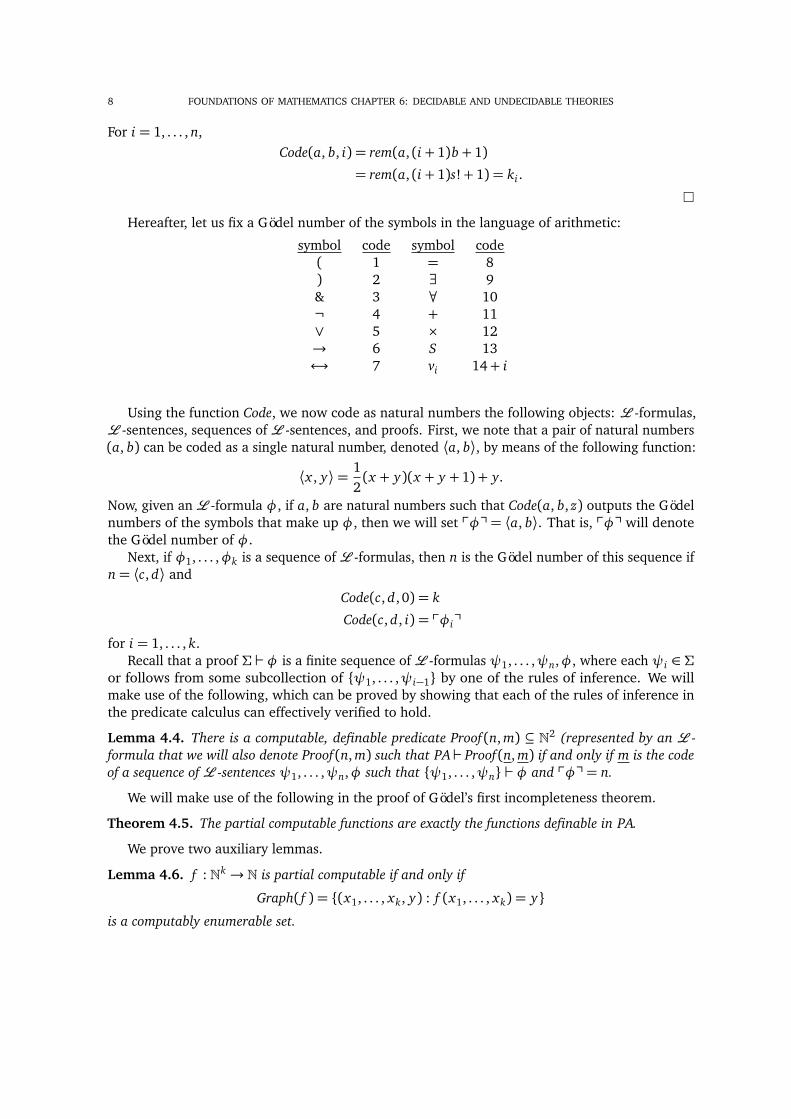
8 FOUNDATIONS OF MATHEMATICS CHAPTER 6: DECIDABLE AND UNDECIDABLE THEORIES
For i = 1, . . . , n,Code(a, b, i) = rem(a, (i + 1)b+ 1)
= rem(a, (i + 1)s!+ 1) = k
i
.
⇤Hereafter, let us fix a Gödel number of the symbols in the language of arithmetic:
symbol code symbol code( 1 = 8) 2 9 9& 3 8 10¬ 4 + 11_ 5 ⇥ 12! 6 S 13$ 7 v
i
14+ i
Using the function Code, we now code as natural numbers the following objects: L -formulas,L -sentences, sequences of L -sentences, and proofs. First, we note that a pair of natural numbers(a, b) can be coded as a single natural number, denoted ha, bi, by means of the following function:
hx , yi= 12(x + y)(x + y + 1) + y.
Now, given an L -formula �, if a, b are natural numbers such that Code(a, b, z) outputs the Gödelnumbers of the symbols that make up �, then we will set �Ò= ha, bi. That is, �Ò will denotethe Gödel number of �.
Next, if �1, . . . ,�k
is a sequence of L -formulas, then n is the Gödel number of this sequence ifn= hc, di and
Code(c, d, 0) = k
Code(c, d, i) = �i
Òfor i = 1, . . . , k.
Recall that a proof ⌃ ` � is a finite sequence of L -formulas 1, . . . , n
,�, where each i
2 ⌃or follows from some subcollection of { 1, . . . ,
i�1} by one of the rules of inference. We willmake use of the following, which can be proved by showing that each of the rules of inference inthe predicate calculus can effectively verified to hold.
Lemma 4.4. There is a computable, definable predicate Proof(n, m) ✓ N2(represented by an L -
formula that we will also denote Proof(n, m) such that PA` Proof(n, m) if and only if m is the code
of a sequence of L -sentences 1, . . . , n
,� such that { 1, . . . , n
} ` � and �Ò= n.
We will make use of the following in the proof of Gödel’s first incompleteness theorem.
Theorem 4.5. The partial computable functions are exactly the functions definable in PA.
We prove two auxiliary lemmas.
Lemma 4.6. f : Nk! N is partial computable if and only if
Graph( f ) = {(x1, . . . , x
k
, y) : f (x1, . . . , x
k
) = y}is a computably enumerable set.
FOUNDATIONS OF MATHEMATICS CHAPTER 6: DECIDABLE AND UNDECIDABLE THEORIES 9
Proof. ()) If f is partial computable, then we can define an effective procedure that enumeratesa tuple (n1, . . . , n
k
, m) into Graph( f ) whenever we see f (n1, . . . , n
k
)#= m.
(() To compute f (n1, . . . , n
k
), enumerate Graph( f ) until we see some tuple (n1, . . . , n
k
, m) thatbelongs to Graph( f ). If no such tuple exists, then we will wait forever and hence f (n1, . . . , n
k
)". ⇤Lemma 4.7. S ✓ Nk
is computably enumerable if and only if there is a computable relation R ✓ Nk+1
such that
S = {(n1, . . . , n
k
) : 9z R(n1, . . . , n
k
, z)}.We will omit the proof this lemma.
Proof of Theorem 4. ((): Suppose that f : Nk ! N is definable in PA. Then there is some L -formula �
f
such that for all u1, . . . , u
k
, v 2 N,
PA` �(u1, . . . , u
k
, v), f (u1, . . . , u
k
) = v
, (u1, . . . , u
k
, v) 2 Graph( f ).
However, PA` �(u1, . . . , u
k
, v) if and only if there is some finite X ✓ PA such that X ` �(u1, . . . , u
k
, v).Equivalently, there is some m such that Proof(m,�
f
(u1, . . . , u
k
, v)Ò) holds (where m codes a se-quence 1, . . . ,
j
,�f
(u1, . . . , u
k
, v) where { 1, . . . , j
} ` �f
(u1, . . . , u
k
, v)). It follows that
Graph( f ) = {(u1, . . . , u
k
, v) : 9m R(u1, . . . , u
k
, v, m)}where R(u1, . . . , u
k
, v, m) is the computable relation Proof(m,�f
(u1, . . . , u
k
, v)Ò). By Lemma 4.7,Graph( f ) is computably enumerable, and so by Lemma 4.6, f is partial computable.
()) We show all partial computable functions are definable in PA by induction. It is not hardto show that the initial functions are definable.
(1) (Constant function): The defining formula �c
(x , y) for the constant function c(x) = 0 is
(y = 0) & (x = x).
(2) (Projective functions): The defining formula �p
k
j
(x1, . . . , x
k
, y) for the projection function
p
k
j
(x1, . . . , x
k
) = x
j
is
(y = x
j
) & (x1 = x1) & . . . & (xk
= x
k
).
(3) (Successor function): The defining formula�S
(x , y) for the successor function S(x) = x+1is y = S(x).
For the induction step of the proof, we must show that the set of PA-definable functions isclosed under the production rules for the set of partial computable functions.
(4) (Composition): Suppose that f and g1, g2, . . . , g
k
are definable in PA by the formulas �f
and �g1
, . . . ,�g
k
, respectively and that h is the function h(~x) = f (g1(~x), . . . , g
k
(~x)). Thenthe defining formula �
h
(~x , y, z) for h is
(9y1)(9y2) . . . (9y
k
)(�g1(~x , y1) & . . . & �
g
k
(~x , y
k
) & �f
(y1, . . . , y
k
, z)).
(5) (Primitive Recursion): Suppose that f and g are definable in PA by�f
and�g
, respectively,and that h is the function defined by recursion with
h(~x , 0) = f (~x)h(~x , y + 1) = g(~x , y, h(~x , y)).
10 FOUNDATIONS OF MATHEMATICS CHAPTER 6: DECIDABLE AND UNDECIDABLE THEORIES
To define h, we will use a pair of numbers a and b that code up the sequence
h(~x , 0), h(~x , 1), . . . , h(~x , y),
via the function Code, where h(~x , 0) = f (~x) and h(~x , n+ 1) = g(~x , n, h(~x , n)) for everyn< y . Thus the defining formula �
h
(~x , y, z) for h is
(9a)(9b)(�f
(~x , Code(a, b, 1))& (8i < y)(�
g
(~x , i, Code(a, b, i + 1), Code(a, b, i + 2))& (z = Code(a, b, y + 1))).
(6) (Unbounded search): Left to the reader.
Thus the class of functions definable in PA includes all the initial functions and is closed underthe production rules. Therefore every partial computable function is definable in PA. ⇤
The following is a key ingredient of the proofs of the incompleteness theorems.
Lemma 4.8 (Diagonal lemma). Let �(x) be an L -formula with one free variable. Then there is an
L -sentence such that
PA` $ �( Ò).Proof. First, observe that the operation that, given inputs n 2 N and a formula A(x) with one freevariable, outputs A(n) is purely mechanical. Similarly, the operation that, given inputs n 2 N andthe Gödel number of such a formula A(x), outputs A(n)Ò, the Gödel number of A(n), is also purelymechanical, and hence is intuitively computable.
Let subst(A(x)Ò, n) = A(n)Ò be this function, which is partial computable (since it may receiveas input some number that is not the Gödel number of any formula, or the Gödel number of aformula with more than one free variable, etc.). By Theorem 4, there is a formula S(x , y, z) thatdefines subst in PA.
The key observation to make here is that for any L -formula A(x) with one free variable, wecan consider the value subst(A(x)Ò,A(x)Ò). Given �(x) as above, let ✓ (x) be the formula
(9y)(�(y) & S(x , x , y)).
That is, ✓ (x) says “There is some y satisfying � that is obtained by substituting x into the formulawith Gödel number x .” Let k = ✓ (x)Ò and consider the sentence ✓ (k), which has Gödel number✓ (k)Ò. Call this sentence .
Unpacking the sentence ✓ (k), we have
(9y)(�(y) & S(k, k, y))
Moreover, since subst(k, k) = ✓ (k)Ò, one can show that
PA` (8y)(S(k, k, y)$ y = ✓ (k)Ò). (1)
Then by definition of PA` $ (9y)(�(y) & S(k, k, y)).
However, by Equation 1,
PA` $ (9y)(�(y) & y = y = ✓ (k)Ò).Equivalently,
PA` $ �(✓ (k)Ò),

FOUNDATIONS OF MATHEMATICS CHAPTER 6: DECIDABLE AND UNDECIDABLE THEORIES 11
which can be rewritten asPA` $ �( Ò).
⇤One last necessary result that we will state without proof is the following.
Lemma 4.9. Given an L -sentence of the form (9x)�(x), if is true in the standard model of
arithmetic, then is provable in PA. That is,
N |= (9x)�(x), PA` (9x)�(x).Theorem 4.10 (Gödel’s First Incompleteness Theorem). If PA is consistent, then PA is not complete.
That is, there is a sentence G
true in the standard model of arithmetic such that PA 6` G
and
PA 6` ¬ G
.
Proof. We apply the Diagonal Lemma to the formula ¬(9x)Proof(x , y), which we will abbreviateas ¬Prov(y) (Informally, this sentence asserts that there is no proof of the sentence with Gödelnumber y). Thus, there is some L -sentence
G
(the “Gödel sentence") such that
PA` G
$ ¬Prov( G
Ò). (2)
That is, G
is equivalent to the L -sentence that asserts that G
is not provable.We now show that if PA is consistent, then PA 6`
G
and PA 6` ¬ G
. In fact, we will show thatPA `
G
if and only if PA ` ¬ G
, which is clearly impossible if PA is consistent and from whichthe desired conclusion follows.
Observe that PA ` G
if and only if (9n)Proof(n, G
Ò) holds, which is equivalent to PA `(9n)Proof(n,
G
Ò) by Lemma 4.9. This is equivalent to PA` Prov( G
Ò), which is equivalent toPA` ¬
G
by (2).Lastly, if PA is consistent, then N |=
G
. Suppose instead that N |= ¬ G
. Since ¬ G
isequivalent to (9n)Proof(n,
G
Ò), it follows that N |= (9n)Proof(n, G
Ò). But then by Lemma 4.9,it follows that PA ` (9n)Proof(n,
G
Ò), i.e., PA ` Prov( G
Ò). But this implies that PA ` ¬ G
,which we have shown is impossible.
⇤We now turn to Gödel’s second incompleteness theorem. Informally, Gödel’s second theorem
states that if PA is consistent, then it cannot prove that it is consistent. To express this formally, weneed to formalize that statement that PA is consistent within PA. The standard way to do this bythe formula ¬Prov(0= 1Ò).Theorem 4.11 (Godel’s Second Incompleteness Theorem). If PA is consistent, then
PA 6` ¬Prov(0= 1Ò).To prove G2, one can show (with a considerable amount of work) that the proof of G1 can be
carried out entirely within PA. We proved above that if PA is consistent, then PA 6` G
; within PA,this yields
PA` ¬Prov(0= 1Ò)! ¬Prov( G
Ò).By G1, we have
PA` G
$ ¬Prov( G
Ò).It follows from the previous two statements that
PA` ¬Prov(0= 1Ò)! G
.
12 FOUNDATIONS OF MATHEMATICS CHAPTER 6: DECIDABLE AND UNDECIDABLE THEORIES
Thus if PA ` ¬Prov(0 = 1Ò), it would follow that PA ` G
, which is impossible by G1. HencePA 6` ¬Prov(0= 1Ò).
Let us take a more general approach to proving G2. Let B(x) be an L -formula with one freevariable. The following three conditions are referred to as derivability conditions:
(D1) If PA` �, then PA` B(�Ò).(D2) PA` B(�! Ò)! (B(�Ò)! B( Ò)).(D3) PA` B(�Ò)! B(B(�Ò)Ò).
With some effort, one can prove that if we let B(x) be the formula Prov(x), then (D1)-(D3) hold.We can now formulate an abstract version of G2:
Theorem 4.12 (Abstract G2). If B(x) satisfies (D1)-(D3), then PA 6` ¬B(0= 1Ò).To prove this theorem, we will first prove the following, which tells us that PA can only prove
that soundness for sentences that it can prove to hold.
Theorem 4.13 (Löb’s Theorem). If B(x) satisfies (D1)-(D3), then for any L -sentence �, if PA `B(�Ò)! �, then PA` �.
Proof. Suppose that B(x) satisfies (D1)-(D3) and that
PA` B(�Ò)! �. (3)
Let ✓ (y) be the formula B(y)! �. By the Diagonal Lemma there is an L -sentence such that
PA` $ (B( Ò)! �) (4)
and hencePA` ! (B( Ò)! �). (5)
From (5) and (D1) it follows that
PA` B( ! (B( Ò)! �)Ò). (6)
By (D2)PA` B( ! (B( Ò)! �)Ò)! (B( Ò)! B(B( Ò)! �Ò)) (7)
Then by applying modus ponens to (6) and (7), we have
PA` B( Ò)! B(B( Ò)! �Ò). (8)
Again by (D2),PA` B(B( Ò)! �Ò)! (B(B( Ò)Ò)! B(�Ò)). (9)
From (8) and (9) we have
PA` B( Ò)! (B(B( Ò)Ò)! B(�Ò)). (10)
By (D3),PA` B( Ò)! B(B( Ò)Ò), (11)
and so from (10) and (11) we can conclude
PA` B( Ò)! B(�Ò). (12)
By (3) and (12) we havePA` B( Ò)! �. (13)
From (4) and (13) it follows thatPA` . (14)

FOUNDATIONS OF MATHEMATICS CHAPTER 6: DECIDABLE AND UNDECIDABLE THEORIES 13
From (D1) we can infer from (14) that
PA` B( Ò). (15)
Applying modus ponens to (13) and (15) gives the desired conclusion
PA` �.
⇤Proof of Abstract G2. Suppose B(x) satisfies (D1)-(D3) and that PA` ¬B(0= 1Ò). Then
PA` B(0= 1Ò)! �for any L -sentence �. In particular,
PA` B(0= 1Ò)! 0= 1.
Then by Löb’s Theorem, it follows that PA ` 0= 1, which contradicts our assumption that PA isconsistent. Thus PA 6` ¬B(0= 1Ò). ⇤

FOUNDATIONS OF MATHEMATICSCHAPTER 7: ALGORITHMIC RANDOMNESS
1. INTRODUCTION
In this chapter, we will briefly the discuss the basics of the theory of algorithmically randomstrings. Although this is not a topic typically covered in an introduction to the foundations of math-ematics, the theory of algorithmic randomness provides interesting examples of the phenomena ofundecidability and incompleteness that we considered in the previous two chapters.
How exactly do we define a finite binary string to be random? One possibility is to take such astring to be random if it is produced by a paradigmatically random process such as the tosses of afair coin. For some purposes, such a definition is sufficient. For our purposes, however, we wouldlike a definition that picks out a fixed collection of binary strings as the random ones (althoughthis is not quite what the theory of algorithmically random finite strings delivers for us).
As a first step, consider the following binary strings of length 50:
(1) 00000 00000 00000 00000 00000 00000 00000 00000 00000 00000(2) 01010 10101 01010 10101 01010 10101 01010 10101 01010 10101(3) 10100 00011 01010 00110 10110 10001 11110 00011 11101 00011(4) 00100 10000 11111 10110 10101 00010 00100 00101 10100 01100(5) 01001 00101 10101 11111 11010 10100 11110 01111 11111 10010
Although it is possible to obtain each of these strings by tossing an unbiased coin (where we take 0to stand for heads and 1 to stand for tails), it is highly unlikely that we would produce (1) and (2)in this way. In fact, (1) and (2) just do not appear to be the sort of strings produced by the tossesof an unbiased coin. It is less clear whether (3)-(5) can be thus produced. For instance, (3) hasthe same number of 0s and 1s, and since most strings of length 50 have close to the same numberof 0s and 1s, we might surmise that (3) was produced by tossing a fair coin. However, (3) encodesthe parity of the number of words of each of the 50 states in alphabetical order (e.g. ‘Alabama’ hasan odd number of letters and thus corresponds to a ‘0’). Although the digits of (4) are less evenlydistributed than those of (3) (29 0s and 21 1s), this is not inconsistent a random origin. However,once we learn that (4) consists of the first 50 bits of the binary expansion of ⇡, we would still besurprised if we were to produce this string by coin tossing. Lastly, (5) is slightly more biased than(3) or (4), but this was (purportedly) produced by encoding some atmospheric noise as a binarystring (at least according to random.org).
What is the upshot of this discussion? One is that strings that appear to be random such as (3)and (4) are no longer thought to be random when they can be given some simpler description.This is one key idea behind the definition of an algorithmically random string: random strings aredifficult to describe. Here we must exercise some caution: here we consider a description of a stringto be one that allows us to reconstruct the string unambiguously, like a blueprint for reproducingthe string. The other key idea behind the definition of an algorithmically random string is that thedescriptions we consider are computational, given in some way by a Turing machine.
1

2 FOUNDATIONS OF MATHEMATICS CHAPTER 7: ALGORITHMIC RANDOMNESS
2. KOLMOGOROV COMPLEXITY
We now make the above ideas precise by defining the Kolmogorov complexity of string, whichallows us to define the complexity of effectively reproducing that string. We begin with an example.
Example 2.1. We define a Turing machine M : 2<!! 2<! that gives short descriptions of strings ofthe form 1n for n 2 N. Given an input string � 2 2<!, M interprets this as some n 2 N written in(reverse) binary and outputs n 1s. Note that if n = 2k for some k, then the input string representingn will have length k+ 1 and will yield as output a string of length 2k, a considerable gain. Thus,we can think of the input string as a compressed version of the output string.
The previous definition suggests the following definition.
Definition 2.2. Let M : 2<!! 2<! be a Turing machine and let � 2 2<!. We define the Kolmogorovcomplexity of � relative to M to be
C
M
(�) =min{|⌧| : M(⌧)#= �},where |⌧| is the length of ⌧. Moreover, if � /2 ran(M), then we set C
M
(�) =1.
If M(⌧) = �, we can think of ⌧ as an M -description of �. Then C
M
(�) is the length of theshortest M -description of �.
Example 2.3. If, as in the previous example, M(�n
) = 1n, where �n
is the binary representation ofn 2 N, then
C
M
(1n) = blog2(n)c+ 1(and C
M
(�) =1 if � 6= 1n for every n 2 N).
One might reasonably worry here that this measure of complexity is completely dependenton our choice of underlying machine. This worry is not unjustified. However, this worry can bemitigated if we define complexity in terms of a universal Turing machine.
Let (Me
)e2N be a computable enumeration of all Turing machines (effectively coded in some
way). Then we define U : 2<!! 2<! by
U(1e0⌧)' M
e
(⌧)
for every e 2 N and � 2 2<!.
Definition 2.4. The Kolmogorov complexity of � is defined to be
C(�) := C
U
(�) =min{|⌧| : U(⌧)#= �}.To what extent does this definition address the concern with machine dependence? The
following theorem, first proved by Kolmogorov, provides an answer:
Theorem 2.5 (Invariance Theorem). For any Turing machine M : 2<!! 2<!, there is some c 2 Nsuch that
C(�) C
M
(�) + c
for every � 2 2<!.
Proof. Given M : 2<!! 2<!, let e be such that M
e
= M . Then for all ⌧ 2 2<!, U(1e0⌧)' M
e
(⌧).Given � 2 2<!, let �⇤ be the shortest string such that M
e
(�⇤M
) = �. Then C
M
(�) = |�⇤|. SinceU(1e0�⇤) = M
e
(�⇤) = �, it follows that
C(�) |1e0�⇤|= |�⇤|+ e+ 1= C
M
(�) + e+ 1.
The conclusion follows by setting c = e+ 1. ⇤

FOUNDATIONS OF MATHEMATICS CHAPTER 7: ALGORITHMIC RANDOMNESS 3
We now find a simple upper bound for C .
Proposition 2.6. There is some c 2 N such that
C(�) |�|+ c
for every � 2 2<!.
Proof. Let M
id
: 2<!! 2<! be the identity machine, which satisfies M(�) = � for every � 2 2<!.Then by the Invariance Theorem, there is some c 2 N such that
C(�) C
M
id
(�) + c = |�|+ c.
⇤
3. INCOMPRESSIBLE STRINGS
We now formalize the notion of an incompressible string, which will serve as the basis of ourdefinition of random strings.
Definition 3.1. Let c 2 N. We say that � 2 2<! is c-incompressible if
C(�)� |�|� c.
Do c-incompressible strings exist? Let us consider the case that c = 0. Note that � 2 2<! is0-incompressible if for every ⌧ 2 2<! such that U(⌧)# = �, it follows that |⌧|� |�|. We claim thatthere is at least one 0-incompressible string of each length. Let us consider strings of length n.There are
1+ 2+ . . .+ 2n�1 = 2n � 1strings of length < n. Hence, in the worst case, if each string of length < n is mapped by U to aunique string of length n, then one string of length n remains and is hence 0-incompressible. Wenow generalize this line of reasoning to prove the following.
Proposition 3.2. For each c 2 N and n 2 N, there are at least 2n� (2n�c�1) c-incompressible strings
of length n.
Proof. There are1+ 2+ . . .+ 2(n�c)�1 = 2n�c � 1
strings of length < n� c. Thus the number of strings of length n to which U maps a string of length< n� c is at most 2n�c � 1. Hence, the number of strings of length n to which U maps no string oflength < n� c is at least 2n � 2n�c � 1. Since all such strings are c-incompressible, the conclusionfollows. ⇤
Note that 2n � (2n�c � 1) = 2n(1� 2�c) + 1> 2n(1� 2�c). From this we can conclude that foreach n 2 N
— at least 1/2 of the strings of length n are 1-incompressible;— at least 3/4 of the strings of length n are 2-incompressible;— at least 7/8 of the strings of length n are 3-incompressible;— and so on.
Thus, if we consider, say, strings of length 100, 99.9% of them are 10-incompressible; that is atleast 1023/1024 of them have complexity greater than 90. It is thus quite easy to produce such astring: toss a fair coin 100 times, and an overwhelming majority of the time, a 10-incompressiblestring will be produced.

4 FOUNDATIONS OF MATHEMATICS CHAPTER 7: ALGORITHMIC RANDOMNESS
Hereafter, we will identify the random strings with sufficiently incompressible strings. Justhow incompressible? We cannot give a precise answer, but for each c, for sufficiently long c-incompressible strings behave, for all practical purposes, like statistically random strings.
Given that it is easy to randomly produce an incompressible string, we might also ask whetherwe can produce incompressible strings algorithmically. Let S
c
be the collection of c-incompressiblestrings. Is there a computable function f : N! 2<! such that ran( f ) ✓ S
c
?
Definition 3.3. A set S ✓ 2<! is immune if it is infinite and has no infinite computably enumerable
subset.
We will show the following, which immediately implies a negative answer to the above question.
Theorem 3.4. For each c 2 N, the collection of c-incompressible strings is immune.
Proof. Fix c 2 N. First note that Sc
is infinite, since by Proposition 3.2, there is a c-incompressiblestring of every length.
Now suppose that Sc
contains an infinite computably enumerable subset {⌧0,⌧1, . . . }. That is,there is some (total) computable function f : N! 2<! such that f (i) = ⌧
i
for every i. Withoutloss of generality, we can assume that |⌧
i
| |⌧i+1| for every i. Indeed, we can define a function
f̂ : N! 2<! that copies f as long as f enumerates a string with length longer than the lengths ofthe previously enumerated strings. That is, if f enumerates a string of length less than or equal toa previously enumerated string, f̂ will not enumerate this string but will wait for a longer stringto be enumerated by f . Since ran( f̂ ) ✓ ran( f ) ✓ S
c
, we can assume that f has this property(replacing f with f̂ if it does not). Note that |⌧
i
| |⌧i+1| for every i implies that |⌧
i
|� i for everyi.
Now, using the function f , we can define a Turing machine M
f
that maps n (written in binary)to f (n) for each n. Then
C
M
f
(⌧n
) blog2(n)c+ 1
and henceC(⌧
n
) blog2(n)c+ d (1)for some d 2 N. However, since each ⌧
n
is c-incompressible,
C(⌧n
)� |⌧n
|� c � n� c, (2)
where the latter inequality follows from the observation at the end of the previous paragraph. Butfor sufficiently large n,
n� c > blog2(n)c+ d,which, together with (1) and (2), yields a contradiction. Thus, S
c
contains no infinite computablyenumerable subset. ⇤Corollary 3.5. There is no total computable f : N! 2<! whose range consists only of c-incompressible
strings.
Corollary 3.6. The function C : 2<!! N is not computable.
Proof. If we could compute the value C(�) for each � 2 2<!, we could immediately determinewhich strings are c-incompressible (for any fixed c). Then we could define a computable enumera-tion of all c-incompressible strings, which is impossible. ⇤
One other consequence of Theorem 3.4 is that we have a second example of a set that iscomputably enumerable but not computable (the first being the halting problem).

FOUNDATIONS OF MATHEMATICS CHAPTER 7: ALGORITHMIC RANDOMNESS 5
Theorem 3.7. For each c 2 N, the collection of c-compressible strings is computably enumerable but
not computable.
Proof. Recall that a set S ✓ 2<! is computable if and only if S and 2<! � S are both computablyenumerable. Since the collection of c-incompressible strings is immune, it cannot be computablyenumerable. It follows that the collection of c-compressible strings is not computable.
To show that this collection is computably enumerable, observe that � 2 2<! is c-compressibleif and only if
(9⌧)(9s)(U(⌧)# in < s steps & U(⌧) = � & |⌧|< |�|� c).Note that the relation R(�,⌧, s) given by
U(⌧)# in < s steps & U(⌧) = � & |⌧|< |�|� c
is a computable relation. Hence, by a lemma from the previous chapter, the collection of c-compressible strings is computably enumerable.
⇤
4. KOLMOGOROV COMPLEXITY AND INCOMPLETENESS
In this final section, we will prove yet another incompleteness theorem known as Chaitin’sIncompleteness Theorem (CIT), which provides us with infinitely many undecidable sentences inthe language of arithmetic. We also will use CIT to provide a new proof of G2 by formalizing theparadox of the surprise exam (explained below).
In order to prove CIT, we need to express statements about the Kolmogorov complexity ofstrings in Peano arithmetic. First, we define a map # : 2<! ! N, which sends each string to aunique natural number that will serve as its code. Let
#(�) = n, 1·� is the binary expansion of n+ 1,
where 1·� is the string obtained by concatenating 1 and �. Thus we have,
#(✏) = 0
#(0) = 1
#(1) = 2
#(00) = 3
#(01) = 4
#(10) = 5
#(11) = 6...
We also define a map | · | : N! N such that if n = #(�), then |n| is the length of the string �; thatis, |#(�)|= |�|.
Next, to represent Kolmogorov complexity in the language of arithmetic, note that sinceevery partial computable function is definable in PA, there is some formula (x , y) (of the form(9z)✓ (x , y, z), where ✓ has no unbounded quantifiers)) such that
U(�) = ⌧, PA` (#(�), #(⌧)).
Note that C(�) n if and only if there is some ⌧ such that |⌧| = n and U(⌧) = �. Thus, usingour coding of members of 2<! and the representations of | · | and U , we can express this by a
6 FOUNDATIONS OF MATHEMATICS CHAPTER 7: ALGORITHMIC RANDOMNESS
formula in the language of arithmetic; for ease of presentation, we will simply write this formulaas C(�) n. We can now state Chaitin’s Theorem.
Theorem 4.1. If PA is consistent, then there is some L 2 N such that
PA 6` C(�)� L
for any � 2 2<! and hence for all n� L,
PA 6` C(�)� n
for any � 2 2<!.
We first prove a lemma.
Lemma 4.2. If PA is consistent, then for n 2 N and � 2 2<!,
PA` C(�)� n) N |= C(�)� n.
That is, if PA proves that the complexity of � is at least n, then it is really the case that the complexity
of � is at least n.
Proof. Suppose that PA ` C(�) � n but in fact we have that N |= C(�) < n. The sentenceexpressing that C(�)< n has the form (9x)✓ (x). However, in the last chapter, we stated that forany such sentence that
N |= (9x)✓ (x)) PA` (9x)✓ (x).Hence PA` C(�)< n, but this contradicts our assumption that PA is consistent. ⇤Proof of CIT. Suppose that for every n 2 N, there is some � 2 2<! such that
PA` C(�)� n.
We define a machine M : 2<!! 2<! that on input ⌧ enumerates theorems of PA until it finds aproof of C(�)� k for some � and some k > 2|⌧|. Then M outputs �.
If M(⌧)#= �, then PA` C(�)� k for some k > 2|⌧|, and hence by by Lemma 4.2, it followsthat C(�)� k > 2|⌧|. By the Invariance Theorem, there is some d 2 N such that
C(�) C
M
(�) + d
for every � 2 2<!. Now, if we give M some input � with |�| = d, we are guaranteed by our initialassumption to find some � 2 2<! such that C(�)> 2|�| = 2d. However, since M(�)# = � we alsohave
C(�) C
M
(�) + d |�|+ d = 2d,which is impossible. Thus it must be the case that PA can only prove C(�)� n for finitely many n,bounded by some L 2 N. ⇤
Note that whereas Gödel’s first incompleteness theorem gives us one undecidable sentence,Chaitin’s theorem gives us infinitely many. However, the Gödel sentence can be produced com-putably, whereas the undecidable sentences in Chaitin’s theorem cannot be produced computably,as we cannot computably determine the bound L.
We now turn to a version of G2 that follows from CIT. Just as the proof of G1 can be formalizedwithin arithmetic, the proof of CIT can be formalized within arithmetic, resulting in:
PA` ¬Prov(0= 1Ò)! (9L)(8x)(|x |= L! ¬Prov(C(x)� LÒ)).As in the original proof of G2, we assume PA` ¬Prov(0= 1Ò) and derive a contradiction. To doso, we formalize the surprise exam paradox.

FOUNDATIONS OF MATHEMATICS CHAPTER 7: ALGORITHMIC RANDOMNESS 7
Suppose that a teacher tells his/her class, “There will be a surprise exam next week, and youwill be surprised when it comes." The students conclude that there will be no surprise exam on thebasis of the following line of reasoning.
— If the exam were on Friday, then when class ends on Thursday and we have yet to takethe exam, we would know it is on Friday and thus it would not be a surprise.
— If the exam were on Thursday, then when class ends on Wednesday and we have yet totake the exam, since it cannot be on Friday, we would know it is on Thursday and thus itwould not be a surprise.
— Similarly, the exam cannot be on Wednesday nor Tuesday. But if the exam were on Monday,since it cannot be on any other day of the week, we would know that it is on Monday andthus it would not be a surprise.
— Therefore there is no surprise exam next week.The following week, the teacher gives a surprise on Wednesday, and the students are all surprised.
How do we formalize this paradox? Let N be the number of strings � of length L such thatC(�)� L, where L is the bound from CIT (so that PA cannot prove that any string has complexity� L). Note that N 2L. Moreover, we proved that there is one 0-incompressible string of eachlength, and thus N � 1. This argument can be formalized in PA, and hence PA` N � 1.
Here we can think of 2L as corresponding to the days of the week on which the surprise exammight be held, while N corresponds to the day of the week on which the exam is held. Just as thestudents reason in such a way that they cannot determine the day of the week on which the examwill be held, in PA, one can show that PA cannot determine which of the possible values 1, . . . , 2L
N is equal to.That is, we prove inductively for each i = 1, . . . , 2N that if PA` N � i, then PA` N � i + 1. We
will not fully write out the formal details here (the full details can be found here). For the basecase, we already have that PA` N � 1. Suppose now that PA` N � i.
(1) First, PA can prove that if N = i then there are 2L � i distinct strings � with C(�)< L.(2) Since PA proves all true statements of the form C(�)< L, it follows that PA can prove that
if N = i then it is provable that there are 2L � i distinct strings � with C(�)< L.(3) Moreover, PA can prove that if N � i, then if there are 2L � i distinct strings � with
C(�)< L, there is some string ⌧ with C(⌧)� L.(4) By the derivability conditions (discussed in the proof of G2), it follows that PA can prove
that if N � i is provable, then if it is provable that there are 2L � i distinct strings � withC(�)< L, there it is provable that there is some string ⌧ with C(⌧)� L.
(5) By (2) and (4) one can conclude (using some basic logic) that if PA can prove that if N = i
and it is provable that N � i, then it is provable that there is some string ⌧ with C(⌧)� L.(6) Since PA ` N � i by the inductive hypothesis, it follows that PA proves that N � i is
provable.(7) Hence by (5) and (6), PA proves that if N = i, then it is provable that there is some string
⌧ with C(⌧)� L.(8) Since it is not provable that there is some string ⌧ with C(⌧)� L (by proving CIT within
arithmetic, as discussed above), it follows that PA 6` N = i, and thus PA` N � i + 1.It now follows by induction that PA ` N � 2L + 1, but since N 2L, we also have PA ` N 2L,which is impossible. Thus PA cannot prove its own consistency.