Foundations of Graphs

2Foundations of Graphs

2.1 Introduction

Graphs, which describe pairwise relations between entities, are essential rep-resentations for real-world data from many different domains, including socialscience, linguistics, chemistry, biology, and physics. Graphs are widely utilizedin social science to indicate the relations between individuals. In chemistry,chemical compounds are denoted as graphs with atoms as nodes and chemicalbonds as edges (Bonchev, 1991). In linguistics, graphs are utilized to capturethe syntax and compositional structures of sentences. For example, parsingtrees are leveraged to represent the syntactic structure of a sentence accordingto some context-free grammar, while Abstract Meaning Representation (AMR)encodes the meaning of a sentence as a rooted and directed graph (Banarescuet al., 2013). Hence, research on graphs has attracted immense attention frommultiple disciplines. In this chapter, we first introduce basic concepts of graphsand discuss the matrix representations of graphs, including adjacency matrixand Laplacian matrix (Chung and Graham, 1997) and their fundamental prop-erties. Then we introduce attributed graphs where each node is associated withattributes and provide a new understanding of these graphs by regarding the at-tributes as functions or signals on the graph (Shuman et al., 2013). We presentthe concepts of graph Fourier analysis and graph signal processing, which layessential foundations for deep learning on graphs. Next, we describe variouscomplex graphs that are frequently utilized to capture complicated relationsamong entities in real-world applications. Finally, we discuss representativecomputational tasks on graphs that have been broadly served as downstreamtasks for deep learning on graphs.

17

18 Foundations of Graphs

2.2 Graph Representations

In this section, we introduce the definition of graphs. We focus on simple un-weighted graphs and will discuss more complex graphs in the following sec-tions.

Definition 2.1 (Graph) A graph can be denoted as G = {V,E}, where V =

{v1, . . . , vN} is a set of N = |V| nodes and E = {e1, . . . , eM} is a set of M edges.

Nodes are essential entities in a graph. In social graphs, users are viewedas nodes, while in chemical compound graphs, chemical atoms are treated asnodes. The size of a given graph G is defined by its number of nodes, i.e.,N = |V|. The set of edges E describes the connections between nodes. An edgee ∈ E connects two nodes v1

e and v2e ; thus, the edge e can be also represented as

(v1e , v

2e). In directed graphs, the edge is directed from node v1

e to node v2e . While

in undirected graphs, the order of the two nodes does not make a difference,i.e., e = (v1

e , v2e) = (v2

e , v1e). Note that without specific mention, we limit our

discussion to undirected graphs in this chapter. The nodes v1e and v2

e are incidentto the edge e. A node vi is adjacent to another node v j if and only if there existsan edge between them. In social graphs, different relations such as friendshipcan be viewed as edges between nodes, and chemical bonds are considered asedges in chemical compound graphs (we regard all chemical bonds as edgeswhile ignoring their different types). A graph G = {V,E} can be equivalentlyrepresented as an adjacency matrix, which describes the connectivity betweenthe nodes.

Definition 2.2 (Adjacency Matrix) For a given graph G = {V,E}, the corre-sponding adjacency matrix is denoted as A ∈ {0, 1}N×N . The i, j-th entry of theadjacency matrix A, indicated as Ai, j, represents the connectivity between twonodes vi and v j. More specifically, Ai, j = 1 if vi is adjacent to v j, otherwiseAi, j = 0.

In an undirected graph, a node vi is adjacent to v j, if and only if v j is adja-cent to vi, thus Ai, j = A j,i holds for all vi and v j in the graph. Hence, for anundirected graph, its corresponding adjacency matrix is symmetric.

Example 2.3 An illustrative graph with 5 nodes and 6 edges is shown in Fig-ure 2.1. In this graph, the set of nodes is represented asV = {v1, v2, v3, v4, v5},and the set of edges is E = {e1, e2, e3, e4, e5, e6}. Its adjacency matrix can bedenoted as follows:

2.3 Properties and Measures 19

𝑣"

𝑣#𝑣$

𝑣%

𝑣& 𝑒#

𝑒$

𝑒"

𝑒%

𝑒&

𝑒(

Figure 2.1 A graph with 5 nodes and 6 edges

A =

0 1 0 1 11 0 1 0 00 1 0 0 11 0 0 0 11 0 1 1 0

2.3 Properties and Measures

Graphs can have varied structures and properties. In this section, we discussbasic properties and measures for graphs.

2.3.1 Degree

The degree of a node v in a graph G indicates the number of times that a nodeis adjacent to other nodes. We have the following formal definition.

Definition 2.4 (Degree) In a graph G = {V,E}, the degree of a node vi ∈ V

is the number of nodes that are adjacent to vi.

d(vi) =∑v j∈V

1E({vi, v j}),


where 1E(·) is an indicator function:

1E({vi, v j}) =

{1 if (vi, v j) ∈ E,0 if (vi, v j) < E.

The degree of a node vi inG can also be calculated from its adjacency matrix.More specifically, for a node vi, its degree can be computed as:

d(vi) =

N∑j=1

Ai, j. (2.1)

Example 2.5 In the graph shown in Figure 2.1, the degree of node v5 is 3,as it is adjacent to 3 other nodes (i.e., v1, v3 and v4). Furthermore, the 5-th rowof the adjacency matrix has 3 non-zero elements, which also indicates that thedegree of v5 is 3.

Definition 2.6 (Neighbors) For a node vi in a graph G = {V,E}, the set of itsneighbors N(vi) consists of all nodes that are adjacent to vi.

Note that for a node vi, the number of nodes in N(vi) equals to its degree,i.e., d(vi) = |N(vi)|.

Theorem 2.7 For a graph G = {V,E}, its total degree, i.e., the summation ofthe degree of all nodes, is twice the number of edges in the graph.∑

vi∈V

d(vi) = 2 · |E|.

Proof ∑vi∈V

d(vi) =∑vi∈V

∑v j∈V

1E({vi, v j})

=∑{vi,v j}∈E

2 · 1E({vi, v j})

= 2 ·∑{vi,v j}∈E

1E({vi, v j})

= 2 · |E|

�

Corollary 2.8 The number of non-zero elements in the adjacency matrix isalso twice the number of the edges.

Proof The proof follows Theorem 2.7 by using Eq. (2.1). �


Example 2.9 For the graph shown in Figure 2.1, the number of edges is 6.The total degree is 12 and the number of non-zero elements in its adjacentmatrix is also 12.

2.3.2 Connectivity

Connectivity is an important property of graphs. Before discussing connectiv-ity in graphs, we first introduce some basic concepts such as walk and path.

Definition 2.10 (Walk) A walk on a graph is an alternating sequence of nodesand edges, starting with a node and ending with a node where each edge isincident with the nodes immediately preceding and following it.

A walk starting at node u and ending at node v is called a u-v walk. Thelength of a walk is the number of edges in this walk. Note that u-v walks arenot unique since there exist various u-v walks with different lengths.

Definition 2.11 (Trail) A trail is a walk whose edges are distinct.

Definition 2.12 (Path) A path is a walk whose nodes are distinct.

Example 2.13 In the graph shown in Figure 2.1, (v1, e4, v4, e5, v5, e6, v1, e1, v2)is a v1-v2 walk of length 4. It is a trail but not a path as it visits node v1 twice.Meanwhile, (v1, e1, v2, e2, v3) is a v1-v3 walk. It is a trail as well as a path.

Theorem 2.14 For a graph G = {E,V} with the adjacency matrix A, we useAn to denote the n-th power of the adjacency matrix. The i, j-th element of thematrix An equals to the number of vi-v j walks of length n.

Proof We can prove this theorem by induction. For n = 1, according to thedefinition of the adjacency matrix, when Ai, j = 1, there is an edge betweennodes vi and v j, which is regarded as a vi-v j walk of length 1. When Ai, j = 0,there is no edge between vi and v j, thus there is no vi-v j walk of length 1.Hence, the theorem holds for n = 1. Assume that the theorem holds whenn = k. In other words, the i, h-th element of Ak equals to the number of vi-vh walks of length k. We then proceed to prove the case when n = k + 1.Specifically, the i, j-th element of Ak+1 can be calculated by using Ak and A as

Ak+1i, j =

N∑h=1

Aki,h · Ah, j. (2.2)

For each h in Eq. (2.2), the term Aki,h ·Ah, j is non-zero only if both Ak

i,h and Ah, j

are non-zero. We have already known that Aki,h denotes the number of vi-vh

walks of length k while Ah, j indicates the number of the vh-v j walk of length 1.


𝑣"

𝑣#𝑣$

𝑣%

𝑣& 𝑒#

𝑒$

𝑒"

𝑒%

𝑒&

𝑒(𝑣(

𝑣)𝑣*

𝑒)𝑒*

Figure 2.2 A graph with two connected components

Hence, the term Aki,h ·Ah, j counts the number of vi-v j walks of length k +1 with

vh as the second last node in the walk. Thus, when summing over all possiblenodes vh, the i, j-th element of Ak+1 equals to the number of vi-v j walks oflength k + 1, which completes the proof. �

Definition 2.15 (Subgraph) A subgraph G′ = {V′,E′} of a given graph G =

{V,E} is a graph formed with a subset of nodesV′ ⊂ V and a subset of edgesE′ ⊂ E. Furthermore, the subsetV′ must contain all the nodes involved in theedges in the subset E′.

Example 2.16 For the graph shown in Figure 2.1, the subset of nodes V′ =

{v1, v2, v3, v5} and the subset of edges E′ = {e1, e2, e3, e6} form a subgraph ofthe original graph G.

Definition 2.17 (Connected Component) Given a graph G = {V,E}, a sub-graph G′ = {V′,E′} is said to be a connected component if there is at leastone path between any pair of nodes in the graph and the nodes in V′ are notadjacent to any vertices inV/V′.

Example 2.18 A graph with two connected components is shown in Fig-ure 2.2, where the left and right connected components are not connected toeach other.

Definition 2.19 (Connected Graph) A graph G = {V,E} is said to be con-nected if it has exactly one component.

Example 2.20 The graph shown in Figure 2.1 is a connected graph, whilethe graph in Figure 2.2 is not a connected graph.


Given a pair of nodes in a graph, there may exist multiple paths with differentlengths between them. For example, there are 3 paths from node v5 to nodev2 in the graph shown in Figure 2.1: (v5, e6, v1, e1, v2), (v5, e5, v4, e4, v1, e1, v2)and (v5, e3, v3, e2, v2). Among them, (v5, e6, v1, e1, v2) and (v5, e3, v3, e2, v2) withlength 3 are the shortest paths from v5 to v2.

Definition 2.21 (Shortest Path) Given a pair of nodes vs, vt ∈ V in graph G,we denote the set of paths from node vs to node vt as Pst. The shortest pathbetween node vs and node vt is defined as:

pspst = arg min

p∈Pst|p|,

where p denotes a path in Pst with |p| its length and pspst indicates the shortest

path. Note that there could be more than one shortest path between any givenpair of nodes.

The shortest path between a pair of nodes describes important informationbetween them. A collective information of the shortest paths between any pairsof nodes in a graph indicates important characteristics of the graph. Specifi-cally, the diameter of a graph is defined as the length of the longest shortestpath in the graph.

Definition 2.22 (Diameter) Given a connected graphG = {V,E}, its diameteris defined as follows:

diameter(G) = maxvs,vt∈V

minp∈Pst

|p|.

Example 2.23 For the connected graph shown in Figure 2.1, its diameter is3. In detail, the longest shortest paths are between node v2 and node v4.

2.3.3 Centrality

In a graph, the centrality of a node measures the importance of the node in thegraph. There are different ways to measure node importance. In this section,we introduce various definitions of centrality.

Degree CentralityIntuitively, a node can be considered as important if there are many other nodesconnected to it. Hence, we can measure the centrality of a given node basedon its degree. In particular, for node vi, its degree centrality can be defined as


follows:

cd(vi) = d(vi) =

N∑j=1

Ai, j.

Example 2.24 For the graph shown in Figure 2.1, the degree centrality fornodes v1 and v5 is 3, while the degree centrality for nodes v2, v3 and v4 is 2.

Eigenvector CentralityWhile the degree based centrality considers a node with many neighbors as im-portant, it treats all the neighbors equally. However, the neighbors themselvescan have different importance; thus they could affect the importance of the cen-tral node differently. The eigenvector centrality (Bonacich, 1972, 2007) definesthe centrality score of a given node vi by considering the centrality scores ofits neighboring nodes as:

ce(vi) =1λ

N∑j=1

Ai, j · ce(v j),

which can be rewritten in a matrix form as:

ce =1λ

A · ce, (2.3)

where ce ∈ RN is a vector containing the centrality scores of all nodes in the

graph. We can reform Eq. (2.3) as:

λ · ce = A · ce.

Clearly, ce is an eigenvector of the matrix A with its corresponding eigenvalueλ. However, given an adjacency matrix A, there exist multiple pairs of eigen-vectors and eigenvalues. Usually, we want the centrality scores to be positive.Hence, we wish to choose an eigenvector with all positive elements. Accord-ing to PerronFrobenius theorem (Perron, 1907; Frobenius et al., 1912; Pillaiet al., 2005), a real squared matrix with positive elements has a unique largesteigenvalue and its corresponding eigenvector has all positive elements. Thus,we can choose λ as the largest eigenvalue and its corresponding eigenvector asthe centrality score vector.

Example 2.25 For the graph shown in Figure 2.1, its largest eigenvalue is2.481 and its corresponding eigenvector is [1, 0.675, 0.675, 0.806, 1]. Hence,the eigenvector centrality scores for the nodes v1, v2, v3, v4, v5 are 1, 0.675, 0.675,0.806,and 1, respectively. Note that the degrees of nodes v2, v3 and v4 are 2;however, the eigenvector centrality of node v4 is higher than that of the other


two nodes as it directly connects to nodes v1 and v5 whose eigenvector central-ity is high.

Katz CentralityThe Katz centrality is a variant of the eigenvector centrality, which not onlyconsiders the centrality scores of the neighbors but also includes a small con-stant for the central node itself. Specifically, the Katz centrality for a node vi

can be defined as:

ck(vi) = α

N∑j=1

Ai, jck(v j) + β, (2.4)

where β is a constant. The Katz centrality scores for all nodes can be expressedin the matrix form as:

ck = αAck + β

(I − α · A)ck = β (2.5)

where ck ∈ RN denotes the Katz centrality score vector for all nodes while β

is the vector containing the constant term β for all nodes. Note that the Katzcentrality is equivalent to the eigenvector centrality if we set α = 1

λmaxand

β = 0, with λmax the largest eigenvalue of the adjacency matrix A. The choiceof α is important – a large α may make the matrix I − α · A ill-conditionedwhile a small α may make the centrality scores useless since it will assign verysimilar scores close to β to all nodes. In practice, α < 1

λmaxis often selected,

which ensures that the matrix I −α ·A is invertible and ck can be calculated as:

ck = (I − α · A)−1β.

Example 2.26 For the graph shown in Figure 2.1, if we set β = 1 and α = 15 ,

the Katz centrality score for nodes v1 and v5 is 2.16, for nodes v2 and v3 is 1.79and for node v4 is 1.87.

Betweenness CentralityThe aforementioned centrality scores are based on connections to neighboringnodes. Another way to measure the importance of a node is to check whetherit is at an important position in the graph. Specifically, if there are many pathspassing through a node, it is at an important position in the graph. Formally,we define the betweenness centrality score for a node vi as:

cb(vi) =∑

vs,vi,vt

σst(vi)σst

, (2.6)


where σst denotes the total number of shortest paths from node vs to node vt

while σst(vi) indicates the number of these paths passing through the node vi.As suggested by Eq. (2.6), we need to compute the summation over all possiblepairs of nodes for the betweenness centrality score. Therefore, the magnitudeof the betweenness centrality score scales as the size of graph scales. Hence, tomake the betweenness centrality score comparable across different graphs, weneed to normalize it. One effective way is to divide the betweenness score bythe largest possible betweenness centrality score given a graph. In Eq. (2.6), themaximum of the betweenness score can be reached when all the shortest pathsbetween any pair of nodes passing through the node vi. That is σst(vi)

σst= 1, ∀vs ,

vi , vt. There are, in total, (N−1)(N−2)2 pairs of nodes in an undirected graph.

Hence, the maximum betweenness centrality score is (N−1)(N−2)2 . We then define

the normalized betweenness centrality score cnb(vi) for the node vi as:

cnb(vi) =

2∑

vs,vi,vt

σst(vi)σst

(N − 1)(N − 2),

Example 2.27 For the graph shown in Figure 2.1, the betweenness centralityscore for nodes v1 and v5 is 3

2 , and their normalized betweenness score is 14 .

The betweenness centrality score for nodes v2 and v3 is 12 , and their normalized

betweenness score is 112 . The betweenness centrality score for node v4 is 0 and

its normalized score is also 0.

2.4 Spectral Graph Theory

Spectral graph theory studies the properties of a graph through analyzing theeigenvalues and eigenvectors of its Laplacian matrix. In this section, we in-troduce the Laplacian matrix of a graph and then discuss its key properties,eigenvalues, and eigenvectors.

2.4.1 Laplacian Matrix

In this subsection, we introduce the Laplacian matrix of a graph, which is an-other matrix representation for graphs in addition to the adjacency matrix.

Definition 2.28 (Laplacian Matrix) For a given graph G = {V,E} with A asits adjacency matrix, its Laplacian matrix is defined as:

L = D − A, (2.7)

where D is a diagonal degree matrix D = diag(d(v1), . . . , d(vN)).

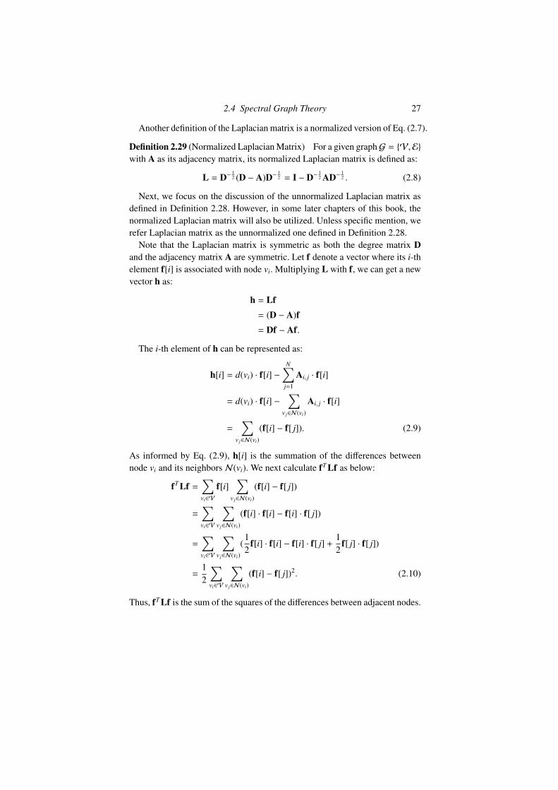
2.4 Spectral Graph Theory 27

Another definition of the Laplacian matrix is a normalized version of Eq. (2.7).

Definition 2.29 (Normalized Laplacian Matrix) For a given graphG = {V,E}

with A as its adjacency matrix, its normalized Laplacian matrix is defined as:

L = D−12 (D − A)D−

12 = I − D−

12 AD−

12 . (2.8)

Next, we focus on the discussion of the unnormalized Laplacian matrix asdefined in Definition 2.28. However, in some later chapters of this book, thenormalized Laplacian matrix will also be utilized. Unless specific mention, werefer Laplacian matrix as the unnormalized one defined in Definition 2.28.

Note that the Laplacian matrix is symmetric as both the degree matrix Dand the adjacency matrix A are symmetric. Let f denote a vector where its i-thelement f[i] is associated with node vi. Multiplying L with f, we can get a newvector h as:

h = Lf= (D − A)f= Df − Af.

The i-th element of h can be represented as:

h[i] = d(vi) · f[i] −N∑

j=1

Ai, j · f[i]

= d(vi) · f[i] −∑

v j∈N(vi)

Ai, j · f[i]

=∑

v j∈N(vi)

(f[i] − f[ j]). (2.9)

As informed by Eq. (2.9), h[i] is the summation of the differences betweennode vi and its neighbors N(vi). We next calculate fT Lf as below:

fT Lf =∑vi∈V

f[i]∑

v j∈N(vi)

(f[i] − f[ j])

=∑vi∈V

∑v j∈N(vi)

(f[i] · f[i] − f[i] · f[ j])

=∑vi∈V

∑v j∈N(vi)

(12

f[i] · f[i] − f[i] · f[ j] +12

f[ j] · f[ j])

=12

∑vi∈V

∑v j∈N(vi)

(f[i] − f[ j])2. (2.10)

Thus, fT Lf is the sum of the squares of the differences between adjacent nodes.


In other words, it measures how different the values of adjacent nodes are. It iseasy to verify that fT Lf is always non-negative for any possible choice of a realvector f, which indicates that the Laplacian matrix is positive semi-definite.

2.4.2 The Eigenvalues and Eigenvectors of the Laplacian Matrix

In this subsection, we discuss main properties of eigenvalues and eigenvectorsof the Laplacian matrix.

Theorem 2.30 For a graph G = {V,E}, the eigenvalues of its Laplacianmatrix L are non-negative.

Proof Suppose that λ is an eigenvalue of the Laplacian matrix L and u is thecorresponding normalized eigenvector. According to the definition of eigenval-ues and eigenvectors, we have λu = Lu. Note that u is a unit non-zero vectorand we have uT u = 1. Then,

λ = λuT u = uTλu = uT Lu ≥ 0

�

For a graph G with N nodes, there are, in total, N eigenvalues/eigenvectors(with multiplicity). According to Theorem 2.30, all the eigenvalues are non-negative. Furthermore, there always exists an eigenvalue that equals to 0. Letus consider the vector u1 = 1

√N

(1, . . . , 1). Using Eq. (2.9), we can easily verifythat Lu1 = 0 = 0u1, which indicates that u1 is an eigenvector correspondingto the eigenvalue 0. For convenience, we arrange these eigenvalues in non-decreasing order as 0 = λ1 ≤ λ2 ≤, . . . ,≤ λN . The corresponding normalizedeigenvectors are denoted as u1, . . . ,uN .

Theorem 2.31 Given a graph G, the number of 0 eigenvalues of its Lapla-cian matrix L (the multiplicity of the 0 eigenvalue) equals to the number ofconnected components in the graph.

Proof Suppose that there are K connected components in the graph G. Wecan partition the set of nodes V into K disjoint subsets V1, . . . ,VK . We firstshow that there exist at least K orthogonal eigenvectors corresponding to theeigenvalue 0. Construct K vectors u1, . . . ,uK such that ui[ j] = 1

√|Vi |

if v j ∈ Vi

and 0 otherwise. We have that Lui = 0 for i = 1, . . . ,K, which indicates thatall the K vectors are the eigenvectors of L corresponding to eigenvalue 0. Fur-thermore, it is easy to validate that uT

i u j = 0 if i , j, which means that theseK eigenvectors are orthogonal to each other. Hence, the multiplicity of the 0eigenvalue is at least K. We next show that there are at most K orthogonal

2.5 Graph Signal Processing 29

eigenvectors corresponding to the eigenvalue 0. Assume that there exists an-other eigenvector u∗ corresponding to the eigenvalue 0, which is orthogonalto all the K aforementioned eigenvectors. As u∗ is non-zero, there must ex-ist an element in u∗ that is non-zero. Let us assume that the element is u∗[d]associated with node vd ∈ Vi. Furthermore, according to Eq.(2.10), we have

u∗T Lu∗ =12

∑vi∈V

∑v j∈N(vi)

(u∗[i] − u∗[ j])2.

To ensure u∗T Lu∗ = 0, the values of nodes in the same component must bethe same. It indicates that all nodes in Vi have the same value u∗[d] as nodevd. Hence, uT

i u∗ > 0. It means u∗ is not orthogonal to ui, which leads to acontradiction. Therefore, there is no more eigenvector corresponding to theeigenvalue 0 beyond the K vectors we have constructed. �

2.5 Graph Signal Processing

In many real-world graphs, there are often features or attributes associated withnodes. This kind of graph-structured data can be treated as graph signals, whichcaptures both the structure information (or connectivity between nodes) anddata (or attributes at nodes). A graph signal consists of a graph G = {V,E},and a mapping function f defined in the graph domain, which maps the nodesto real values. Mathematically, the mapping function can be represented as:

f : V → R1×d,

where d is the dimension of the value (vector) associated with each node. With-out loss of generality, in this section, we set d = 1 and denote the mappedvalues for all nodes as f ∈ RN with f[i] corresponding to node vi.

Example 2.32 A graph signal is shown in Figure 2.3, where the color of anode represents its associated value with smaller values tending toward blueand larger values tending toward red.

A graph is smooth if the values in connected nodes are similar. A smoothgraph signal is with low frequency, as the values change slowly across thegraph via the edges. The Laplacian matrix quadratic form in Eq. (2.10) can beutilized to measure the smoothness (or the frequency) of a graph signal f as itis the summation of the square of the difference between all pairs of connectednodes. Specifically, when a graph signal f is smooth, fT Lf is small. The valuefT Lf is called as the smoothness (or the frequency) of the signal f.


-0.8

-0.6

-0.4

-0.2

0

0.2

0.4

0.6

0.8

Figure 2.3 A one-dimensional graph signal

In the classical signal processing setting, a signal can be denoted in two do-mains, i.e., the time domain and the frequency domain. Similarly, the graphsignal can also be represented in two domains, i.e., the spatial domain, whichwe just introduced, and the spectral domain (or frequency domain). The spec-tral domain of graph signals is based on the Graph Fourier Transform. It isbuilt upon the spectral graph theory that we have introduced in the previoussection.

2.5.1 Graph Fourier Transform

The classical Fourier Transform (Bracewell, n.d.)

f (ξ) =< f (t), exp(−2πitξ) >=

∞∫−∞

f (t) exp(−2πitξ)dt

decomposes a signal f (t) into a series of complex exponentials exp(−2πitξ)for any real number ξ, where ξ can be viewed as the frequency of the corre-sponding exponential. These exponentials are the eigenfunctions of the one-dimensional Laplace operator (or the second order differential operator) as we

2.5 Graph Signal Processing 31

have

∇(exp(−2πitξ)) =∂2

∂t2 exp(−2πitξ)

=∂

∂t(−2πiξ) exp(−2πitξ)

= −(2πiξ)2 exp(−2πitξ).

Analogously, the Graph Fourier Transform for a graph signal f on graph Gcan be represented as:

f[l] =< f,ul >=

N∑i=1

f[i]ul[i], (2.11)

where ul is the l-th eigenvector of the Laplacian matrix L of the graph. Thecorresponding eigenvalue λl represents the frequency or the smoothness of theeigenvector ul. The vector f with f[l] as its l-th element is the Graph FourierTransform of f. The eigenvectors are the graph Fourier basis of the graph G,and f consists of the graph Fourier coefficients corresponding to these basis fora signal f. The Graph Fourier Transform of f can be also denoted in the matrixform as:

f = U>f (2.12)

where the l-th column of the matrix U is ul.As suggested by the following equation:

u>l Lul = λl · u>l ul = λl,

the eigenvalue λl measures the smoothness of the corresponding eigenvectorul. Specifically, the eigenvectors associated with small eigenvalues vary slowlyacross the graph. In other words, the values of such eigenvector at connectednodes are similar. Thus, these eigenvectors are smooth and change with lowfrequency across the graph. However, the eigenvectors corresponding to largeeigenvalues may have very different values on two nodes, even if connected.An extreme example is the first eigenvector u1 associated with the eigenvalue0 – it is constant over all the nodes, which indicates that its value does notchange across the graph. Hence, it is extremely smooth and has an extremelylow frequency 0. These eigenvectors are the graph Fourier basis for the graphG, and their corresponding eigenvalues indicate their frequencies. The GraphFourier Transform, as shown in Eq. (2.12) can be regarded as a process todecompose an input signal f into graph Fourier basis with different frequencies.The obtained coefficients f denote how much the corresponding graph Fourierbasis contributes to the input signal.


u1

u15

u30

Graph Fourier Basis

-1

0

1

2

3

4

5

Fre

quency

Figure 2.4 Frequencies of graph Fourier basis

Example 2.33 Figure 2.4 shows the frequencies of the graph Fourier basis ofthe graph shown in Figure 2.3. Note that the frequency of u1 is 0.

The graph Fourier coefficients f are the representation of the signal f in thespectral domain. There is also the Inverse Graph Fourier Transform, which cantransform the spectral representation f to the spatial representation f as:

f[i] =

N∑l=1

f [l]ul[i].

This process can also be represented in the matrix form as follows:

f = Uf.

In summary, a graph signal can be denoted in two domains, i.e., the spatialdomain and the spectral domain. The representations in the two domains canbe transformed to each other via the Graph Fourier Transform and the InverseGraph Fourier Transform, respectively.

Example 2.34 Figure 2.5 shows a graph signal in both the spatial and spectraldomains. Specifically, Figure 2.5a shows the graph signal in the spatial domainand Figure 2.5b illustrates the same graph signal in the spectral domain. InFigure 2.5b, the x-axis is the graph Fourier basis and the y-axis indicates thecorresponding graph Fourier coefficients.

2.6 Complex Graphs 33

-0.8

-0.6

-0.4

-0.2

0

0.2

0.4

0.6

0.8

(a) A graph signal in the spatial domain

0 1 2 3 4 5

0.5

1

1.5

2

2.5

(b) A graph signal in the spectral domain

Figure 2.5 Representations of a graph signal in both spatial and spectral Domains

2.6 Complex Graphs

In the earlier sections, we introduced simple graphs and their fundamentalproperties. However, graphs in real-world applications are much more compli-cated. In this section, we briefly describe popular complex graphs with formaldefinitions.

2.6.1 Heterogeneous Graphs

The simple graphs we have discussed are homogeneous. They only have onetype of nodes as well as a single type of edges. However, in many real-worldapplications, we want to model multiple types of relations between multipletypes of nodes. As shown in Figure 2.6, in an academic network describingpublications and citations, there are three types of nodes, including authors,papers, and venues. There are also various kinds of edges denoting differentrelations between the nodes. For example, there exist edges describing thecitation relations between papers or edges denoting the authorship relationsbetween authors and papers. Next, we formally define heterogeneous graphs.

Definition 2.35 (Heterogeneous Graphs) A heterogeneous graph G consistsof a set of nodes V = {v1, . . . , vN} and a set of edges E = {e1, . . . , eM} whereeach node and each edge are associated with a type. Let Tn denote the setof node types and Te indicate the set of edge types. There are two mappingfunctions φn : V → Tn and φe : V → Te that map each node and each edge totheir types, respectively.


published_at

paper

cite

authored

conference

author

attend

Figure 2.6 A heterogeneous academic graph

2.6.2 Bipartite Graphs

In a bipartite graph G = {V,E}, its node set V can be divided into two dis-joint subsets V1 and V2 where every edge in E connects a node in V1 to anode in V2. Bipartite graphs are widely used to capture interactions betweendifferent objects. For example, as shown in Figure 2.7, in many e-commerceplatforms such as Amazon, the click history of users can be modeled as a bi-partite graph where the users and items are the two disjoint node sets, andusers’ click behaviors form the edges between them. Next, we formally definebipartite graphs.

Definition 2.36 (Bipartite Graph) Given a graph G = {V,E}, it is bipartite ifand only if V = V1 ∪ V2, V1 ∩ V2 = ∅ and v1

e ∈ V1 while v2e ∈ V2 for all

e = (v1e , v

2e) ∈ E.

2.6.3 Multi-dimensional Graphs

In many real-world graphs, multiple relations can simultaneously exist be-tween a pair of nodes. One example of such graph can be found at the pop-ular video-sharing site YouTube, where users are viewed as nodes. YouTubeusers can subscribe to each other, which is considered as one relation. Userscan be connected via other relations such as “sharing” or “commenting” videosfrom other users. Another example is from e-commerce sites such as Amazon,


Figure 2.7 An e-commerce bipartite graph

where users can interact with items through various types of behaviors such as“click”, “purchase” and “comment”. These graphs with multiple relations canbe naturally modeled as multi-dimensional graphs by considering each type ofrelations as one dimension.

Definition 2.37 (Multi-dimensional graph) A multi-dimensional graph con-sists of a set of N nodes V = {v1, . . . , vN} and D sets of edges {E1, . . . ,ED}.Each edge set Ed describes the d-th type of relations between the nodes inthe corresponding d-th dimension. These D types of relations can also be ex-pressed by D adjacency matrices A(1), . . . ,A(D). In the dimension d, its cor-responding adjacency matrix A(d) ∈ RN×N describes the edges Ed betweennodes in V. Specifically, the i, j-th element of Ad, denoted as A(d)

i, j , equals to1 only when there is an edge between nodes vi and v j in the dimension d (or(vi, v j) ∈ Ed), otherwise 0.


unfriend

unfriend

friend

friend

friend

friend

Figure 2.8 An illustrative signed graph

2.6.4 Signed Graphs

Signed graphs, which contain both positive and negative edges, have becomeincreasingly ubiquitous with the growing popularity of the online social net-works. Examples of signed graphs are from online social networks such asFacebook and Twitter, where users can block or unfollow other users. The be-haviour of “block” can be viewed as negative edges between users. Meanwhile,the behaviour of “unfriend” can also be treated as negative edges. An illustra-tive example of a signed graph is shown in Figure 2.8, where users are nodesand “unfriend” and “friend” relations are the “negative” and “positive” edges,respectively. Next, we give the formal definition of signed graphs.

Definition 2.38 (Signed Graphs) Let G = {V,E+,E−} be a signed graph,where V = {v1, . . . , vN} is the set of N nodes while E+ ⊂ V × V and E− ⊂V×V denote the sets of positive and negative edges, respectively. Note that anedge can only be either positive or negative, i.e., E+ ∩ E− = ∅. These positiveand negative edges between nodes can also be described by a signed adjacencymatrix A, where Ai, j = 1 only when there is a positive edge between node vi

and node v j, Ai, j = −1 denotes a negative edge, otherwise Ai, j = 0.


Author 1

Author 2

Author 3

Figure 2.9 An illustrative hypergraph

2.6.5 Hypergraphs

The graphs we introduced so far only encode pairwise information via edges.However, in many real-world applications, relations are beyond pairwise as-sociations. Figure 2.9 demonstrates a hypergraph describing the relations be-tween papers. An specific author can publish more than two papers. Thus, theauthor can be viewed as a hyperedge connecting multiple papers (or nodes).Compared with edges in simple graphs, hyperedges can encode higher-orderrelations. The graphs with hyperedges are called as hypergraphs. Next, we givethe formal definition of hypergraphs.

Definition 2.39 (Hypergraphs) Let G = {V,E,W} be a hypergraph, whereV is a set of N nodes, E is a set of hyperedges and W ∈ R|E|×|E| is a diagonalmatrix with W[ j, j] denoting the weight of the hyperedge e j. The hypergraphG can be described by an incidence matrix H ∈ R|V|×|E|, where Hi, j = 1 onlywhen the node vi is incident to the edge e j. For a node vi, its degree is defined as

d(vi) =|E|∑j=1

Hi, j, while the degree for a hyperedge is defined as d(e j) =|V|∑i=1

Hi, j.

Furthermore, we use De and Dv to denote the diagonal matrices of the edgeand node degrees, respectively.

2.6.6 Dynamic Graphs

The graphs mentioned above are static, where the connections between nodesare fixed when observed. However, in many real-world applications, graphs areconstantly evolving as new nodes are added to the graph, and new edges are


𝑡"𝑡#

𝑡$

𝑡%

𝑡&

𝑡'

𝑡(

𝑡)𝑣$

𝑣%

𝑣& 𝑣'

𝑣(

𝑣)𝑣"𝑣+

Figure 2.10 An illustrative example of dynamic graphs.

continuously emerging. For example, in online social networks such as Face-book, users can constantly establish friendships with others, and new users canalso join Facebook at any time. These kinds of evolving graphs can be denotedas dynamic graphs where each node or edge is associated with a timestamp.An illustrative example of dynamic graphs is shown in Figure 2.10, where eachedge is associated with a timestamp, and the timestamp of a node is when thevery first edge involves the node. Next, we give a formal definition of dynamicgraphs.

Definition 2.40 (Dynamic Graphs) A dynamic graph G = {V,E}, consistsof a set of nodes V = {v1, . . . , vN} and a set of edges E = {e1, . . . , eM} whereeach node and/or each edge is associated with a timestamp indicating the timeit emerged. Specifically, we have two mapping functions φv and φe mappingeach node and each edge to their emerging timestamps.

In reality, we may not be able to record the timestamp of each node and/oreach edge. Instead, we only check from time to time to observe how the graphevolves. At each observation timestamp t, we can record the snapshot of thegraph Gt as the observation. We refer to this kind of dynamic graphs as dis-crete dynamic graphs, which consist of multiple graph snapshots. We formallydefine the discrete dynamic graph as follows.

Definition 2.41 (Discrete Dynamic Graphs) A discrete dynamic graph con-sists of T graph snapshots, which are observed along with the evolution of a dy-

2.7 Computational Tasks on Graphs 39

namic graph. Specifically, the T graph snapshots can be denoted as {G0, . . . ,GT }

where G0 is the graph observed at time 0.

2.7 Computational Tasks on Graphs

There are a variety of computational tasks proposed for graphs. These taskscan be mainly divided into two categories. One is node-focused tasks, wherethe entire data is usually represented as one graph with nodes as the data sam-ples. The other is graph-focused tasks, where data often consists of a set ofgraphs, and each data sample is a graph. In this section, we briefly introducerepresentative tasks for each group.

2.7.1 Node-focused Tasks

Numerous node-focused tasks have been extensively studied, such as nodeclassification, node ranking, link prediction, and community detection. Next,we discuss two typical tasks, including node classification and link prediction.

Node classificationIn many real-world graphs, nodes are associated with useful information, oftentreated as labels of these nodes. For example, in social networks, such infor-mation can be demographic properties of users such as age, gender, and occu-pation, or users’ interests and hobbies. These labels usually help characterizethe nodes and can be leveraged for many important applications. For example,in social media such as Facebook, labels related to interests and hobbies canbe utilized to recommend relevant items (i.e., news and events) to their users.However, in reality, it is often difficult to get a full set of labels for all nodes.For example, less than 1% of Facebook users provide their complete demo-graphic properties. Hence, we are likely given a graph with only a part of thenodes associated with labels, and we aim to infer the labels for nodes withoutlabels. It motivates the problem of node classification on graphs.

Definition 2.42 (Node classification) Let G = {V,E} denote a graph withVthe set of nodes and E the set of edges. Some of the nodes inV are associatedwith labels, and the set of these labeled nodes is represented as Vl ⊂ V. Theremaining nodes do not have labels, and this set of unlabeled nodes is denotedasVu. Specifically, we haveVl ∪ Vu = V andVl ∩ Vu = ∅. The goal of thenode classification task is to learn a mapping φ by leveraging G and labels ofVl, which can predict the labels of unlabeled nodes (or v ∈ Vu).


The above definition is for simple graphs that can be easily extended tographs with attributes and complex graphs we introduced in Section 2.6.

Example 2.43 (Node Classification in Flickr) Flickr is an image hosting plat-form that allows users to host their photos. It also serves as an online socialcommunity where users can follow each other. Hence, users in Flickr and theirconnections form a graph. Furthermore, users in Flickr can subscribe to in-terest groups such as “Black and White”, “The Fog and The Rain”, and “DogWorld”. These subscriptions indicate the interests of users and can be used astheir labels. A user can subscribe to multiple groups. Hence, each user can beassociated with multiple labels. A multi-label node classification problem ongraphs can help predict the potential groups that users are interested in, but theyhave not yet subscribed to. One such dataset on Flickr can be found in (Tangand Liu, 2009).

Link PredictionIn many real-world applications, graphs are not complete but with missingedges. Some of the connections exist. However, they are not observed or recorded,which leads to missing edges in the observed graphs. Meanwhile, many graphsare naturally evolving. In social media such as Facebook, users can continu-ously become friends with other users. In academic collaboration graphs, agiven author can constantly build new collaboration relations with other au-thors. Inferring or predicting these missing edges can benefit many applicationssuch as friend recommendation (Adamic and Adar, 2003), knowledge graphcompletion (Nickel et al., 2015), and criminal intelligence analysis (Berlus-coni et al., 2016). Next, we give the formal definition of the link predictionproblem.

Definition 2.44 (Link Prediction) Let G = {V,E} denote a graph with Vas its set of nodes and E as its set of edges. Let M denote all possible edgesbetween nodes inV. Then, we denote the complementary set of E with respectto M as E′ = M/E. The set E′ contains the unobserved edges between thenodes. The goal of the link prediction task is to predict the edges that mostlikely exist. Specifically, a score can be assigned to each of the edges in E′. Itindicates how likely the edge exists or will emerge in the future.

Note that the definition is stated for simple graphs and can be easily ex-tended to complex graphs we introduced in Section 2.6. For example, forsigned graphs, in addition to the existence of an edge, we also want to pre-dict its sign. For hypergraphs, we want to infer hyperedges which describe therelations between multiple nodes.

2.7 Computational Tasks on Graphs 41

Example 2.45 (Predicting Emerging Collaborations in DBLP) DBLP is anonline computer science bibliography website that hosts a comprehensive listof research papers in computer science. A co-authorship graph can be con-structed from the papers in DBLP, where the authors are the nodes, and authorscan be considered as connected if they have co-authored at least one paper asrecorded in DBLP. Predicting what new collaborations between authors whonever co-authored before is an interesting link prediction problem. A largeDBLP collaboration dataset for link prediction research can be found in (Yangand Leskovec, 2015).

2.7.2 Graph-focused Tasks

There are numerous graph-focused tasks, such as graph classification, graphmatching, and graph generation. Next, we discuss the most representative graph-focused task, i.e., graph classification.

Graph ClassificationNode classification treats each node in a graph as a data sample and aimsto assign labels to these unlabeled nodes. In some applications, each samplecan be represented as a graph. For example, in chemoinformatics, chemicalmolecules can be denoted as graphs where atoms are the nodes, and chemicalbonds between them are the edges. These chemical molecules may have dif-ferent properties such as solubility and toxicity, which can be treated as theirlabels. In reality, we may want to predict these properties for newly discov-ered chemical molecules automatically. This goal can be achieved by the taskof graph classification, which aims to predict the labels for unlabeled graphs.Graph classification cannot be carried out by traditional classification due tothe complexity of graph structures. Thus, dedicated efforts are desired. Next,we provide a formal definition of graph classification.

Definition 2.46 (Graph Classification) Given a set of labeled graphs D =

{(Gi, yi)} with yi as the label of the graph Gi, the goal of the graph classificationtask is to learn a mapping function φ with D, which can predict the labels ofunlabeled graphs.

In the definition above, we did not specify additional information poten-tially associated with the graphs. For example, in some scenarios, each nodein a graph is associated with certain features that can be utilized for graphclassification.

Example 2.47 (Classifying Proteins into Enzymes or Non-enzymes) Proteins


can be represented as graphs, where amino acids are the nodes, and edgesbetween two nodes are formed if they are less than 6A apart. Enzymes are atype of proteins which serve as biological catalysts to catalyze biochemicalreactions. Given a protein, predicting whether it is an enzyme or not can betreated as a graph classification task where the label for each protein is eitherenzyme or non-enzyme.

2.8 Conclusion

In this chapter, we briefly introduced the concepts of graphs, the matrix rep-resentations of graphs, and the important measures and properties of graphs,including degree, connectivity, and centrality. We then discuss Graph FourierTransform and graph signal processing, which lay the foundations for spectralbased graph neural networks. We introduce a variety of complex graphs. Fi-nally, we discuss representative computational tasks on graphs, including bothnode-focused and graph-focused tasks.

2.9 Further Reading

We briefly introduce many basic concepts in graphs. There are also other moreadvanced properties and concepts in graphs such as flow and cut. Furthermore,there are many problems defined on graphs, including graph coloring prob-lem, route problem, network flow problem, and covering problem. These con-cepts and topics are covered by the books (Bondy et al., n.d.; Newman, 2018).Meanwhile, more spectral properties and theories on graphs can be found in thebook (Chung and Graham, 1997). Applications of graphs in different areas canbe found in (Borgatti et al., 2009; Nastase et al., 2015; Trinajstic, 2018). TheStanford Large Network Dataset Collection (Leskovec and Krevl, 2014) andthe Network Data Repository (Rossi and Ahmed, 2015), host large amountsof graph datasets from various areas. The python libraries networkx (Hag-berg et al., 2008), graph-tool (Peixoto, 2014), and SNAP (Leskovec and Sosic,2016) can be used to analyze and visualize graph data. The Graph Signal Pro-cessing Toolbox (Perraudin et al., 2014) can be employed to perform graphsignal processing.

Documents

Foundations of Graphs