SANDIA REPORT SAND2006-4634 Unlimited Release Printed July 2006

Forward Osmosis: A New Approach to Water Purification and Desalination James E. Miller and Lindsey R. Evans Prepared by Sandia National Laboratories Albuquerque, New Mexico 87185 and Livermore, California 94550 Sandia is a multiprogram laboratory operated by Sandia Corporation, a Lockheed Martin Company, for the United States Department of Energy’s National Nuclear Security Administration under Contract DE-AC04-94AL85000. Approved for public release; further dissemination unlimited.

2

Issued by Sandia National Laboratories, operated for the United States Department of Energy by Sandia Corporation. NOTICE: This report was prepared as an account of work sponsored by an agency of the United States Government. Neither the United States Government, nor any agency thereof, nor any of their employees, nor any of their contractors, subcontractors, or their employees, make any warranty, express or implied, or assume any legal liability or responsibility for the accuracy, completeness, or usefulness of any information, apparatus, product, or process disclosed, or represent that its use would not infringe privately owned rights. Reference herein to any specific commercial product, process, or service by trade name, trademark, manufacturer, or otherwise, does not necessarily constitute or imply its endorsement, recommendation, or favoring by the United States Government, any agency thereof, or any of their contractors or subcontractors. The views and opinions expressed herein do not necessarily state or reflect those of the United States Government, any agency thereof, or any of their contractors. Printed in the United States of America. This report has been reproduced directly from the best available copy. Available to DOE and DOE contractors from U.S. Department of Energy Office of Scientific and Technical Information P.O. Box 62 Oak Ridge, TN 37831 Telephone: (865) 576-8401 Facsimile: (865) 576-5728 E-Mail: reports@adonis.osti.gov Online ordering: http://www.osti.gov/bridge Available to the public from U.S. Department of Commerce National Technical Information Service 5285 Port Royal Rd. Springfield, VA 22161 Telephone: (800) 553-6847 Facsimile: (703) 605-6900 E-Mail: orders@ntis.fedworld.gov Online order: http://www.ntis.gov/help/ordermethods.asp?loc=7-4-0#online

3

SAND2006-4634 Unlimited Release Printed July 2006

Forward Osmosis: A New Approach to

Water Purification and Desalination

James E. Miller and Lindsey R. Evans Sandia National Laboratories

P.O. Box 5800 Albuquerque, NM 87185-1349

Abstract

Fresh, potable water is an essential human need and thus looming water shortages threaten the world’s peace and prosperity. Waste water, brackish water, and seawater have great potential to fill the coming requirements. Unfortunately, the ability to exploit these resources is currently limited in many parts of the world by both the cost of the energy and the investment in equipment required for purification/desalination. Forward (or direct) osmosis is an emerging process for dewatering aqueous streams that might one day help resolve this problem. In FO, water from one solution selectively passes through a membrane to a second solution based solely on the difference in the chemical potential (concentration) of the two solutions. The process is spontaneous, and can be accomplished with very little energy expenditure. Thus, FO can be used, in effect, to exchange one solute for a different solute, specifically chosen for its chemical or physical properties. For desalination applications, the salts in the feed stream could be exchanged for an osmotic agent specifically chosen for its ease of removal, e.g. by precipitation. This report summarizes work performed at Sandia National Laboratories in the area of FO and reviews the status of the technology for desalination applications. At its current state of development, FO will not replace reverse osmosis (RO) as the most favored desalination technology, particularly for routine waters. However, a future role for FO is not out of the question. The ability to treat waters with high solids content or fouling potential is particularly attractive. Although our analysis indicates that FO is not cost effective as a pretreatment for conventional BWRO, water scarcity will likely drive societies to recover potable water from increasingly marginal resources, for example gray water and then sewage. In this context, FO may be an attractive pretreatment alternative. To move the technology forward, continued improvement and optimization of membranes is recommended. The identification of optimal osmotic agents for different applications is also suggested as it is clear that the space of potential agents and recovery processes has not been fully explored.

4

This page intentionally left blank

5

Table of Contents 1. Introduction..................................................................................................................... 7

1.1 Water is a National Security Issue ............................................................................ 7 1.2 The Desalination Landscape ..................................................................................... 7

2. Forward Osmosis .......................................................................................................... 10 2.1 The Forward Osmosis Landscape........................................................................... 10 2.2 Membranes for Forward Osmosis........................................................................... 12 2.3 Osmotic Agents....................................................................................................... 14

3. Applying Forward Osmosis to Desalination................................................................ 14 3.1 Initial Design Concept .......................................................................................... 14 3.2 Osmotic Agents for Initial Design Concept............................................................ 16 3.3 Experimentation on Initial Design Concept............................................................ 18

3.3.1 Screening Osmotic Agents............................................................................... 18 3.3.2 Membrane Screening and Demonstration of Concept ..................................... 22

3.3.2.2 Hydrophobic Hollow Fiber Membrane Contactor.................................... 23 3.3.2.3 Flat Sheet Membrane Testing ................................................................... 26

3.3.3 Putting it all Together ...................................................................................... 31 3.3.3.1 Best Case Thermal Osmotic Agent and Recoveries ................................. 31 3.3.3.2 Best Case Membrane and Why Improvements are Needed...................... 31 3.3.3.3 Thermodynamics (Ideal) of the Best Case Scenario................................. 34 3.3.3.4 Summary Evaluation of Initial Process Design ........................................ 35

3.4 Chemical Precipitation............................................................................................ 36 3.5 Salts of Carboxylic Acids and Carbon Dioxide...................................................... 37

4. The Cost of Using FO as a Pretreatment Technology .................................................. 41 5. Late Breaking News...................................................................................................... 44 6. Concluding Remarks and Recommendations ............................................................... 46 7. References..................................................................................................................... 46

List of Figures

Figure 1. Cost breakdown for RO desalination of brackish water. Adapted from [14].... 9 Figure 2. Cost breakdown for RO desalination of seawater. Adapted from [15]. ............ 9 Figure 3. Flow of water across a semi-permeable membrane from solution with high chemical potential (low salt concentration) to low chemical potential (high salt concentration). .................................................................................................................. 10 Figure 4. Process schematic for osmotic concentration of heat sensitive solutions. Figure adapted from [24].............................................................................................................. 11 Figure 5. Block diagram illustrating strategy for applying FO and thermal precipitation of an osmotic agent (AB, Table 1) to accomplish desalination. ....................................... 15 Figure 6. Osmotic pressure (solid) and concentration (dashed) of saturated borax solutions assuming ideal behavior and calculated using experimentally derived values for ∆H and ∆S. For approximate borax concentration in g/100 cc, multiply molar concentration by 38........................................................................................................... 17 Figure 7. At any temperature greater than 20 °C, the osmotic pressure of a saturated Na2HPO4 should exceed that of seawater (3.5% NaCl). Data assumes van’t Hoff behavior............................................................................................................................. 22 Figure 8. Celgard X-50 membrane contactor. ................................................................. 23

6

Figure 9. Schematic diagram of membrane testing apparatus. ........................................ 24 Figure 10. Flux across X-50 membrane contactor with NaCl solutions on shell side, and DI water on lumen side. Osmotic pressure calculated using van’t Hoff equation........... 24 Figure 11. Flux across X-50 membrane contactor with Na2HPO4 solutions on shell side, and DI water or NaCl on lumen side. ............................................................................... 25 Figure 12. Assembled membrane testing apparatus. ....................................................... 26 Figure 13. Disassembled membrane testing apparatus showing flow channels. ............. 26 Figure 14. Performance of Osmotek 011105a membrane in tests of Na2HPO4 (10-45 wt%) vs. 3.5 wt% NaCl. Driving force calculated using van’t Hoff equation. Squares indicate data points taken in repeat later (duplicate) experiments. ................................... 29 Figure 15. Flux from 3.5% NaCl solution through 0.45 µm Gore-Tex membrane as a function of temperature and Na2HPO4 concentration....................................................... 30 Figure 16. Osmotic pressure (assuming ideal behavior) as a function of concentration for NaCl and Na2HPO4 solutions............................................................................................ 31 Figure 17. Schematic diagram of FO process using Na2HPO4 as the osmotic agent and “leaky” membranes requiring purge stream. .................................................................... 32 Figure 18. Schematic diagram of FO process showing secondary precipitation step to limit loss of osmotic agent to purge stream. ..................................................................... 34 Figure 19. Solubility data for Na2HPO4 (see inset of Figure 11) plotted to determine ∆H and ∆S for dissolution (assumes Na2HPO4 = 2 Na+ + HPO4

2-, and neglects data at higher temperatures where solubility is no longer a strong function of temperature). ................ 35 Figure 22. Relationship between CO2 pressure and pH for a soy meal extract solution. 38

List of Tables

Table 1. Osmotic pressure of a saturated solution of hypothetical salt AB with an endothermic heat of dissolution of 24 kcal/mol and entropy change on dissolution of 0.07 kcal/mol compare to a 3.5% NaCl solution. ..................................................................... 15 Table 2. Examples of Potential Osmotic Agents from CRC [55].................................... 18 Table 3. Solubility of calcium hydrogen malate: Ca(C4H5O5)2 [54]. ............................. 19 Table 4. Solubility of calcium malate: CaC4H4O5 [54]. ................................................. 19 Table 5. Solubility of sodium tetra-decanoate [54]. ........................................................ 20 Table 6. Solubility of disodium orthophosphate Na2HPO4 [54]...................................... 20 Table 7. Boiling points and Osmotic Pressures (calculated at the boiling point, from the boiling point) of different test solutions............................................................................ 21 Table 8. Impact of various operating variables on steady state salt accumulation and loss of osmotic agent to purge stream resulting from back diffusion of salt into osmotic agent............................................................................................................................................ 33 Table 9. Solubilities of select calcium and magnesium carboxylate salts. ...................... 40 Table 10. Solubility as function of temperature for 3-5-dihyroxybenzoic acid............... 41 Table 11. Specifications of feed water for cost evaluations ............................................ 42

7

1. Introduction 1.1 Water is a National Security Issue Currently, about half of the world’s population suffers from water shortages, and over the next 25 years, the number of people affected by severe water shortages is expected to increase fourfold [1]. In the developing countries that are most affected, 80-90% of all diseases and 30% of all deaths result from poor water quality [2]. In addition, modern economies cannot develop and thrive without sufficient access to water. There is growing recognition by governments and corporations that future peace and prosperity is intimately tied to the availability of clean, fresh water [3,4]. Thus it is that developing low cost methods of purifying freshwater, and desalting seawater is of strategic importance. 1.2 The Desalination Landscape The current state-of-the-art for water purification and desalination is reverse osmosis (RO) [5]. RO is a membrane separation process that recovers pure water from an impure or saline water feed by pressurizing it to a level above its osmotic pressure. In essence, the membrane filters out the salt ions from the pressurized solution, allowing only the water to pass. For any new desalination technology to be commercially viable it must offer significant improvements over RO in at least one of many performance measures. These measures include energy costs, capital costs, water recovery rates, operability and maintenance requirements, water quality, and the product water cost. Each of these factors is considered briefly below. Most of the energy consumed by RO is accounted for by the pressurization of water. Since the minimum pressure required to perform the separation (the osmotic pressure) is directly related to the dissolved salt concentration, RO is most efficient and has lower energy requirements for treating nearly pure or brackish water, where only low to intermediate pressures are required. The operating pressure for brackish water systems ranges from 15 – 25 bar and for seawater systems from 54 to 80 bar (the osmotic pressure of seawater is about 25 bar) [6]. The energy requirements reported for RO purification of seawater are typically about 15-30 kJ/kg of fresh water [5], although values as high as 61 kJ/kg have been reported [7]. Since most of the energy losses for RO result from releasing the pressure of the concentrated brine, large scale RO systems are now equipped with devices to recover the mechanical compression energy from the discharged concentrated brine stream with efficiencies claimed to be up to 95% [8]. In these plants, the energy required for seawater desalination has now been reported to be as low as 9 kJ/kg product [9]. This low value however is more typical of a system treating brackish water. To provide perspective on the energy requirements, the theoretical minimum energy for desalination of seawater is in the range of 3-7 kJ/kg water [10]. Although this number can be arrived at in a number of ways, it is perhaps easiest to think of this number as the energy associated with the process of salt dissolution. When considering energy costs, it is also important to consider how the energy will be provided (i.e. as electricity or fuel) and to consider the cost (or efficiency) of interconversion (e.g. thermal to electrical) as

8

necessary. It is also important to remember that for any real process, there is a tradeoff between capital costs and energy costs that leads to an optimum plant design and minimum product water cost. Spiegler and El-Sayed have recently published reviews of this concept [11]. In short, the best overall process design is not necessarily the most energy efficient design. Keep in mind that for special applications, other design parameters, e.g. size and weight, may also need to be considered. The water recovery rate of RO systems tends to be low. A typical recovery value for a seawater RO system is only 40% [10]. This is generally driven by two considerations: that fact that ever higher pressures (and energy consumption) are required as the brine is concentrated, and the potential for scale formation. There are, however, a number of other considerations that drive the design towards maximizing water recovery. First, significant resources may be required to transport and pretreat the saline feed to the plant. Second, in areas where water is scarce, the water may be too valuable to discard as concentrated brine. Conversely, environmental considerations or brine disposal costs may make it too costly to discard large quantities of brine. In addition, energy losses and inefficiencies in the desalination process tend to increase with increasing water rejection. For example, heat is often rejected from a system with the concentrated brine, and energy is lost when concentrated RO brines are depressurized. Although distillation processes typically produce water of a higher quality than membrane processes, this is generally not an issue for most applications. The safe limit for the salinity of drinking water is usually about 1000 ppm while the voluntary EPA standard is 500 ppm [12]. These can readily be met in most cases by RO, particularly when one considers that the water may be blended with water from other sources. It is difficult to generalize the cost for RO treatment of water. Many cost factors vary greatly over time, geography, and concentration. This is particularly true for energy costs, although other factors can also be important. For example, the feed water quality influences the cost of pretreatment, and the location of the plant will determine the cost of transporting the water and the cost of disposing of the concentrated brine solution. Other factors such as low interest government financing or subsidies can significantly influence capital and other costs as can the size of the plant. To further complicate matters, it has been pointed out that there is no agreed on standard for computing and reporting water costs [13]. Some authors have chosen to neglect capital costs, some have chosen to report all costs including delivery costs, and some report design costs that do not ultimately reflect actual operating expenses. Despite these caveats, it appears that a well-designed RO plant in the developed world can desalt seawater at a cost in the range of $2 to $4 per 1000 gallons, and it appears to be generally accepted that seawater RO can be carried out in the U.S. for somewhere in the low end of this range [5]. This is generally lower than competing technologies. Figures 1 and 2 provide additional information regarding the contributions of various process aspects to total cost for RO of brackish water and seawater.

9

Fixed Charges - 54%

Consumables - 10%

Electric Power - 11%

Maintenance & Parts - 9%

Labor - 9%

Membrane Replacement - 7%

RO Unit - $1/gal/dayPretreatment – 30% of RO UnitPolishing – 30-50% of RO UnitInstallation – 30% of Total Equipment CostSite – 150% of Total Equipment Cost

Fixed Charges - 54%

Consumables - 10%

Electric Power - 11%

Maintenance & Parts - 9%

Labor - 9%

Membrane Replacement - 7%

RO Unit - $1/gal/dayPretreatment – 30% of RO UnitPolishing – 30-50% of RO UnitInstallation – 30% of Total Equipment CostSite – 150% of Total Equipment Cost

Fixed Charges - 54%

Consumables - 10%

Electric Power - 11%

Maintenance & Parts - 9%

Labor - 9%

Membrane Replacement - 7%

RO Unit - $1/gal/dayPretreatment – 30% of RO UnitPolishing – 30-50% of RO UnitInstallation – 30% of Total Equipment CostSite – 150% of Total Equipment Cost

Figure 1. Cost breakdown for RO desalination of brackish water. Adapted from [14].

Fixed Charges - 37%

Consumables - 3%

Electric Power - 44%

Maintenance & Parts - 7%

Labor - 4%

Membrane Replacement - 5%Fixed Charges - 37%

Consumables - 3%

Electric Power - 44%

Maintenance & Parts - 7%

Labor - 4%

Membrane Replacement - 5%

Figure 2. Cost breakdown for RO desalination of seawater. Adapted from [15]. The main problems associated with RO desalination generally arise in the areas of operability and maintenance. RO membranes are sensitive to pH, oxidizers, a wide range of organics, algae, bacteria and of course particulates and other foulants [16]. Membrane fouling, biofouling in particular, is the source of most problems in RO plants. Fouling, if not addressed in a timely manner, can permanently damage membranes and result in decreases in recovery, increases in energy consumption, or even require membrane replacement. Therefore, pretreatment (or lack thereof) of the feed water is an important consideration and can have a significant impact on the cost of and lifetime of RO [17]. In summary, RO is the current state-of-the-art desalination technology. In a well-designed facility, RO can reliably produce high quality water at a cost of $2 to $4 per 1000 gallons with an energy expenditure in the range of 10-60 kJ/kg. This sets a very high bar for competing technologies to meet. Nonetheless, there is some room for

10

improvement. Accounting for conversion of thermal energy to electric energy, RO requires at least 9 times the theoretical minimum energy required to desalt seawater. In addition, the water recovery rate of RO systems tends to be low, and the membranes are subject to degradation and fouling. 2. Forward Osmosis 2.1 The Forward Osmosis Landscape As implied above, osmosis is the spontaneous flow of a solvent, generally water, across a membrane that is permeable by the solvent, but not the solutes (a semi-permeable

membrane). The driving force for flow is a difference in the chemical potential on the two sides of the membrane (Figure 3), with the solvent moving from a region of higher potential (generally a lower solute concentration) to lower potential (higher solute concentration). Osmosis can only occur if the membrane can differentiate between solvent and solute; otherwise, mixing will occur. The concept of osmotic pressure is used to characterize the potential of a solution for osmosis. In practical terms, the osmotic pressure of a solution is the pressure that must be applied to the solution to stop the net flow from a pure solvent across the membrane into the solution. In the ideal case, the osmotic pressure is directly proportional to the concentration of the solute:

π=nRT n=[sum of all ions in solution]

Since osmotic pressure results from the chemical potential, it is directly relatable to other solution properties such as boiling point elevation and freezing point depression. We proposed that forward (direct) osmosis (FO) could be applied to create a new paradigm for desalination that focuses on behavior of the solute, reasoning that with this approach we could more closely approach theoretical efficiencies. Our

specific proposal was to employ forward osmosis to, in effect, exchange the numerous salts found in seawater (e.g. NaCl and MgCl) for a single, specifically chosen, “designer” solute. Since this exchange occurs spontaneously as the result of a gradient in osmotic pressure it can, in

theory, be achieved for virtually no energy cost above that which would be required in any system to pump water. Our plan was to choose the designer solution so that the solute is easily and directly separated from the extracted water (e.g. by precipitation) with

Figure 3. Flow of water across a semi-permeable membrane from solution with high chemical potential (low salt concentration) to low chemical potential (high salt concentration).

ContaminatedFlow (µA)

Osmotic Solution (µB)

Diffusion

µA > µB

ContaminatedFlow (µA)

Osmotic Solution (µB)

Diffusion

µA > µB

11

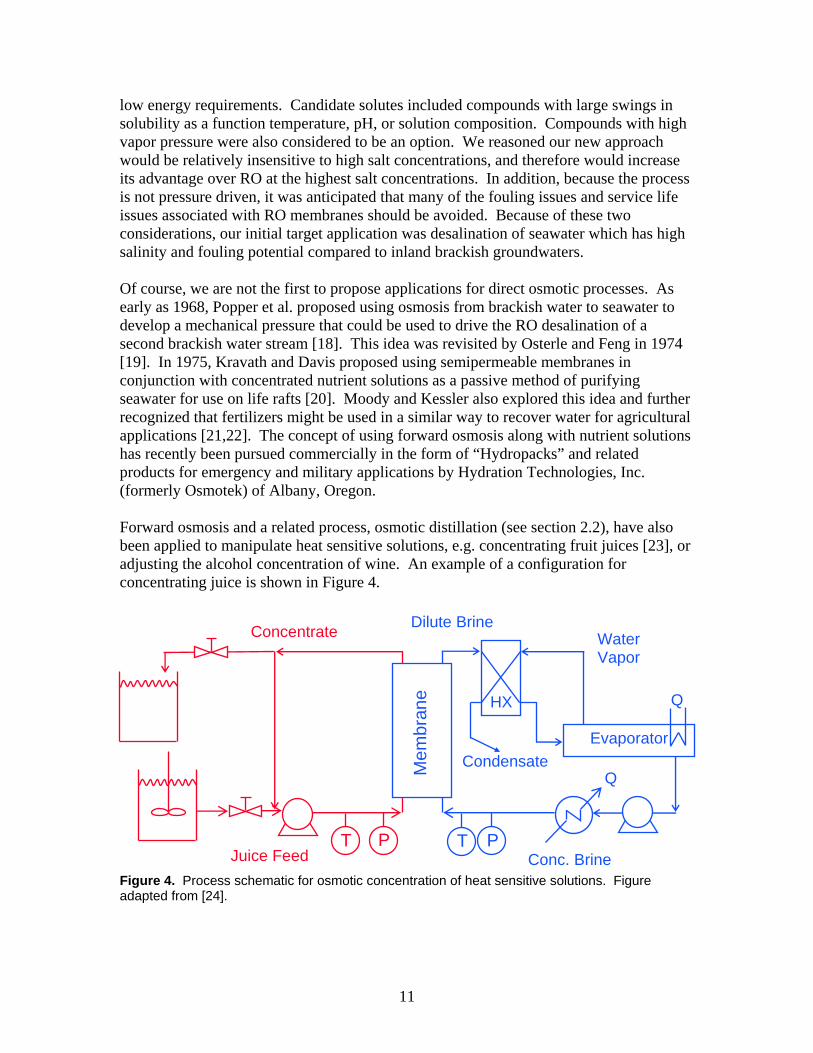
low energy requirements. Candidate solutes included compounds with large swings in solubility as a function temperature, pH, or solution composition. Compounds with high vapor pressure were also considered to be an option. We reasoned our new approach would be relatively insensitive to high salt concentrations, and therefore would increase its advantage over RO at the highest salt concentrations. In addition, because the process is not pressure driven, it was anticipated that many of the fouling issues and service life issues associated with RO membranes should be avoided. Because of these two considerations, our initial target application was desalination of seawater which has high salinity and fouling potential compared to inland brackish groundwaters. Of course, we are not the first to propose applications for direct osmotic processes. As early as 1968, Popper et al. proposed using osmosis from brackish water to seawater to develop a mechanical pressure that could be used to drive the RO desalination of a second brackish water stream [18]. This idea was revisited by Osterle and Feng in 1974 [19]. In 1975, Kravath and Davis proposed using semipermeable membranes in conjunction with concentrated nutrient solutions as a passive method of purifying seawater for use on life rafts [20]. Moody and Kessler also explored this idea and further recognized that fertilizers might be used in a similar way to recover water for agricultural applications [21,22]. The concept of using forward osmosis along with nutrient solutions has recently been pursued commercially in the form of “Hydropacks” and related products for emergency and military applications by Hydration Technologies, Inc. (formerly Osmotek) of Albany, Oregon. Forward osmosis and a related process, osmotic distillation (see section 2.2), have also been applied to manipulate heat sensitive solutions, e.g. concentrating fruit juices [23], or adjusting the alcohol concentration of wine. An example of a configuration for concentrating juice is shown in Figure 4.

Figure 4. Process schematic for osmotic concentration of heat sensitive solutions. Figure adapted from [24].

PTT

Concentrate Water Vapor

Mem

bran

e

Juice Feed Conc. Brine P

Evaporator

HX

Condensate

Dilute Brine

Q

Q

12

In the scheme shown in Figure 4, the fruit juice and a concentrated solution of an osmotic agent are circulated on opposite sides of a membrane. Water flows out of the juice to dilute the osmotic agent, thereby concentrating the juice. The osmotic agent is reconcentrated in an evaporator and recirculated. This has the effect of displacing the thermal step to the osmotic agent and preserves the quality (flavor) of the concentrate. For these applications, the osmotic agent would be chosen based on cost and toxicity and would generally be something like table salt or sugar. These types of systems have been operated with high solids contents, without pretreatment, lending credence to the idea that FO could be advantageous for treating waters with high fouling potential. In addition to food-related applications, osmotic processes have also been applied to concentrate other difficult streams including landfill leachate, and industrial process wastes [25]. Of course, osmosis is very important in biological systems and the principles can be applied to artificial dialysis or to time- or targeted-released pharmaceuticals [26]. One of the more intriguing, if not yet practical, applications considered for forward osmosis is the generation of electrical power. Because energy is released when freshwater mixes with saline water (recall the chemical potential is higher for pure water than for a salt solution), there is the potential to harvest energy wherever a freshwater flow (e.g. a river) mixes with a saline stream (e.g. the ocean). Conceivably, if a semipermeable membrane were used to separate the two environments, a pressure (equivalent to the difference in the osmotic pressure of the two waters) could be generated to drive a turbine [27]. Applying this concept to the Great Salt Lake, it has been estimated that 130 MW could be generated at a cost of $0.15/kWhr [28].

2.2 Membranes for Forward Osmosis As in an RO process, great demands will be placed on a membrane in an most industrial FO processes. First, the membrane must allow water to flow from the feed (e.g. seawater) to the osmotic solution with virtually no cross contamination of salts. This is important for at least two reasons. First, loss of the osmotic agent to the environment must be minimized to limit the replacement cost and any potential environmental impacts. Second, contamination of the osmotic agent can modify the solubility characteristics, and could ultimately require a periodic purge of the osmotic agent (see section 3.3.3). A second demand placed on the FO membrane is a high rate of water flux across the membrane. It is important to limit the size of the FO unit for reasons of capital costs (number and size of units), and to limit the energy required to pump water through the unit. Additional requirements are that the membrane be stable in the presence of the osmotic agent and at the temperatures of interest. A review of the literature shows that there are at least three approaches to membranes for large scale osmotic (non-RO) concentration processes. The most common approach seems to be the use of microporous hydrophobic membranes, commonly fabricated as hollow fibers [23,29-39], but also available as flat sheets. Processes utilizing these membranes are actually more closely related to a distillation process (direct contact membrane distillation [40]) than they are to an osmotic process and are therefore commonly referred to as osmotic distillation (OD), or osmotic evaporation (OE). Microporous hydrophobic membranes contain a very large number of small pores that penetrate completely through the membrane. Since the hydrophobic membrane is not

13

wetted, water vapor passes through the membrane pores but the aqueous solution is prevented from passing through the pores, provided the pressure is maintained below a critical value. A net flux of water vapor across the membrane will result if there is a partial pressure gradient across the membrane. In OD, both sides of the membrane are contacted with aqueous solutions and the partial pressure gradient is provided by a difference in salt concentrations across the membrane. The partial pressure of water over the solution is related to the osmotic pressure through the following relation:

π = (RT/V)ln(Po/P) where V is the molar volume of water, and Po and P are the vapor pressures of pure water and solution respectively at the temperature of interest [30]. Microporous hydrophobic membranes have the advantage that there is virtually no cross-contamination of salts. Since liquid does not transport across hydrophobic membrane, dissolved ions (with virtually no vapor pressure) are completely rejected. Unfortunately, this high selectivity comes at the price of low flux across the membrane. Typical fluxes are in the range of 0-3 l/m2/hr. For comparison, fluxes across RO membranes can reach 75 l/m2/hr although typical values are 1/2 to 1/3 of this. The low mass transfer rates result from relatively small vapor pressure gradients (equivalent to only small temperature differences [35,36,41]) coupled with small pores sizes and relatively thick membranes. In addition, only a portion of the membrane area is actually available for transport (40% porosity is typical). Another drawback to these membranes is that they tend to lose their hydrophobicity over time as they degrade or become fouled, resulting in liquid transport and cross-contamination [42]. They are also relatively expensive. A second membrane approach to FO is simply to use RO membranes [43]. Although little data has been published on this approach, the main drawback is again limited flux across the membrane. In a recent study, fluxes of up to 3.1 l/m2/hr were reported [44], although with extensive solution pretreatment via ultrafiltration, fluxes were improved to 7.3 l/m2/hr [45]. As was specifically noted in the study, the low fluxes can be primarily traced to the fact that RO membranes are by necessity relatively thick to withstand the rigors of the pressure driven process. A third approach is to design and fabricate new membranes specifically for the FO process. When one considers the fact that the current RO membranes that perform so admirably are the product of at least 40 years of refinement, it is clear that if FO desalination technologies are to be viable, that this is the approach that must be applied. We have only identified a single commercial entity that is pursuing this approach, Osmotek Inc. Osmotek manufactures their membranes to be much thinner than traditional RO membranes, and to be asymmetric with only a very thin tight layer providing the desired selectivity [46-49]. The advantage to this approach is that by tailoring the membrane to the solutions of interest, fluxes can be maximized, while maintaining the desired selectivity. Osmotek has been able to produce optimized membranes with fluxes approaching 20 l/m2/hr. In addition, through proper system design, Osmotek has been able to produce membrane contactors that maintain their high flux rates for feeds with high solids content, without pretreatment.

14

2.3 Osmotic Agents Regardless of the application, osmotic agents should ideally be inert, stable, of neutral or near neutral pH, and non-toxic. They should not degrade the membrane chemically (through reaction, dissolution, or adsorption) or physically (fouling) and should have minimal effects on the environment or human health. They should also be inexpensive, very soluble, and provide a high osmotic pressure. For specific applications, additional criteria will apply. Our desalination concept requires the osmotic agent to be easily (both from a physical and energetic standpoint) and completely recoverable from water. Osmotic agents for desalination are discussed in more detail below. 3. Applying Forward Osmosis to Desalination 3.1 Initial Design Concept In order to achieve our goal of lowering the cost of desalination, the design needed to be simple and elegant with as few process steps as possible, and with little or no consumption of the osmotic agent or other materials. Our initial conceptual design was essentially a process similar to that shown in Figure 4, with the evaporator replaced with a different, less energy intensive, unit operation. Our presumption was that the new unit operation would either be a crystallizer or an air stripper. We assumed that the crystallizer would be used in the case of an osmotic agent whose solubility could be manipulated through temperature or pH, and the stripper would be used if a highly volatile agent was identified. Thermal precipitation of the designer solute from the osmotic solution was considered to be our leading candidate for success. We reasoned that pH adjustment would probably require the consumption of costly acids and bases, and also probably increase the need for a periodic replacement or continual purge of the osmotic agent solution. Also, air stripping can require the circulation of large gas volumes, and recovery of the vapor for reuse can be difficult and costly. Furthermore, the use of volatile agents would restrict the choice of membranes; microporous membranes (osmotic distillation) are inappropriate in this case. To understand how a thermal agent would work, consider a hypothetical binary salt (AB) with an endothermic heat of dissolution of 24 kcal/mol and an entropy change on dissolution of 0.07 kcal/mol. The effect of temperature on the saturation concentration can then be calculated using the well know relations:

∆G = ∆H - T∆S ∆G = -RTlnK, and

K = [A][B] where G, H, and S are Gibbs free energy, enthalpy and entropy respectively, R is ideal gas constant, T is absolute temperature, K is the solubility product, and [A] and [B] are the molar concentrations of ions A and B in solution. Furthermore, for purposes of this illustration, we can estimate the osmotic pressure, π, of different solutions using the simple van’t Hoff equation:

π=RT[sum of all ions in solution] (The van’t Hoff equation is a simplification that strictly applies only to dilute solutions. For a more exact approach to concentrated solutions see the works of Pitzer et al. [50].)

15

Thus, given the thermodynamic parameters of the dissolution process, we can calculate the ion concentration in a saturated solution of AB and the resulting osmotic pressure as a function of temperature. We can also calculate the osmotic pressure of seawater (for our purposes a 3.5% NaCl solution) as a function of temperature. The results are summarized in Table 1. Table 1. Osmotic pressure of a saturated solution of hypothetical salt AB with an endothermic heat of dissolution of 24 kcal/mol and entropy change on dissolution of 0.07 kcal/mol compare to a 3.5% NaCl solution.

Temperature (°C) π (atm) Sat’d AB

π (atm) Seawater

0 0.49 27 25 3.4 29 40 9.6 31 60 32 33 80 96 35

The data from Table 1 are applied to our concept in Figure 5. First seawater and a saturated AB solution are passed at a reasonable, but elevated, temperature of 80 °C in a countercurrent fashion on opposite sides of a forward osmosis membrane. It may be unnecessary to heat the seawater. However, membrane contactors tend to also function as heat exchangers, and heating the seawater would likely be necessary to optimize heat management and system operability. In the contactor, water flows across the membrane from the seawater to the AB solution. Given appropriate membrane kinetics and surface area, the AB solution will be diluted to the point that its osmotic pressure upon leaving the contactor will approach that of the seawater feed. From the table, we can see that the saturation temperature of the AB solution exiting the contactor will be slightly above 60 °C. Thus, the next step is to cool the diluted AB solution to about 60 °C.

Sea Water

Conc.Brine

ForwardOsmosis

HX

Mixer

Precip.

HeatPump/Recovery

VeryConc.

AB

80 °C

DiluteAB

80 °C

DiluteAB60 °C

Q

Q

pptd.AB

5 °C

VeryDilute

AB

ABRecycle25 °C

HX

80 °C

80 °C

Sea Water

Ambient

Conc.Brine

Ambient

LowPress.

RO

Fresh Water

Q

HX25 °C

Q

Sea Water

Conc.Brine

ForwardOsmosis

HXHX

MixerMixer

Precip.

HeatPump/Recovery

HeatPump/Recovery

VeryConc.

AB

80 °C

DiluteAB

80 °C

DiluteAB60 °C

Q

Q

pptd.AB

5 °C

VeryDilute

AB

ABRecycle25 °C

HX

80 °C

80 °C

Sea Water

Ambient

Conc.Brine

Ambient

LowPress.

RO

LowPress.

RO

Fresh Water

Q

HXHX25 °C

Q

Figure 5. Block diagram illustrating strategy for applying FO and thermal precipitation of an osmotic agent (AB, Table 1) to accomplish desalination.

16

The heat from cooling the solution is recovered and used to preheat a recycle stream. The dilute stream is then cooled beyond the saturation point, resulting in the precipitation of AB. This can be accomplished in a number of ways, but the primary requirement is that the heat must be recovered as efficiently as possible for reuse elsewhere. Two streams leave the precipitation apparatus, a solid stream of precipitated AB salt, and a very dilute liquid stream saturated with AB at a low temperature (e.g. 5 °C). The solid is recycled to make up the concentrated stream being fed to the forward osmosis unit. The cool, very dilute solution is passed to a final polishing step (shown in Figure 5 as a low pressure RO or nanofiltration unit) to remove the final traces of salt. Prior to the polishing step the temperature must be slightly raised to prevent precipitation of AB during the polishing step. In addition to freshwater, the polisher produces a low concentration stream of the osmotic agent AB that is recycled back to the forward osmosis unit. In a real system, the requirements for a final polishing step will depend on a number of factors, e.g. the relative effectiveness of the precipitation step, the cost and toxicity of the “designer” osmotic agent, and perhaps a tradeoff between the cost of sub-ambient cooling and operating the polisher. 3.2 Osmotic Agents for Initial Design Concept An analysis of the energy requirements of the conceptual design shows that heat management is essential. This can be aided in part by choosing an osmotic agent with a large swing in solubility over a very small temperature range. Ideally, the osmotic agent would have retrograde solubility. This way a cold rather than warm solution could be fed to the forward osmosis unit, bypassing the need to preheat or lose heat to the seawater. Also, it would possibly eliminate the requirement for subambient cooling, a less energy efficient process than heating. By combining the equations introduced above we arrive at the following: This equation (in the form of a line with slope –∆H/R and intercept ∆S/R) shows that for a salt to show retrograde solubility (decreasing Ksp with an increase in temperature) the heat of dissolution needs to be negative (exothermic). In addition, for there to be a large temperature effect, the heat of dissolution (slope of the line) should be relatively large. For salts, these considerations imply that the ions should have high charge density and thus large heats of hydration. For high solubility, positive changes in entropy are also desirable (negative values will counter the positive heat of dissolution term). Unfortunately, ions that have large charge density and are highly solvated generally have negative values for ∆S. Thus it is that salts with retrograde solubility generally have very low solubility overall and/or solubilities that only vary over a small range with temperature. For salts with the more typical solubility behavior (increasing solubility with temperature) the heat of dissolution will be positive (endothermic). Again, to have a

nKspRS

RTH

l=∆

+∆−

17

relatively large temperature effect, a relatively large value for the heat of dissolution is desirable. However, examining the equation, one can see that this can have the effect of making the overall solubility quite low. This effect must be countered by a positive entropy term. These considerations are generally met by ions with relatively low charge densities. As an example of a potential agent whose solubility is a strong function temperature, consider borax (Na2B4O7•10 H2O, or alternately Na2B4O5(OH)4•8 H2O). The solubility

of borax can readily be measured at different temperatures by titrating with HCl. We titrated solutions in our laboratory that were saturated with borax at temperatures of 25, 50, and 80 °C, and arrived at values of 21.7 kcal/mol and 66.3 cal/molK for ∆H and ∆S, respectively. This data is applied in Figure 6 to calculate an osmotic pressure and concentration for saturated borax solutions as a function of temperature (assuming ideal behavior).

In addition to ionic salts, there are a number of other potential classes of osmotic agents whose temperature/solubility characteristics might be of interest. In particular, calcium salts of organic compounds are of interest because of the potential for retrograde solubility. Surfactants are interesting in that they exhibit large changes in solubility at a distinct temperature (known as the Krafft temperature) where micelle formation becomes possible. In addition, strong intermicellar interactions can lead to unexpectedly high osmotic pressures [51]. However, due to the high molecular weight of the compounds, it appears that the osmotic pressures will in general still be too low for this application. Surfactants also may precipitate as coagels, heterogeneous mixtures of surfactant and water that are sometimes described as opaque suspensions of crystals [52]. Processing coagels would likely pose many difficulties. Organic molecules may also be of interest. In addition to those that precipitate as a solid, those that form a separate liquid phase may also be of interest. For example, the miscibility of triethylamine decreases with increasing temperature. It is also a low boiling compound that might be readily stripped. However, potential problems with this and other low molecular weight compounds are toxicity, flammability, and potential

Figure 6. Osmotic pressure (solid) and concentration (dashed) of saturated borax solutions assuming ideal behavior and calculated using experimentally derived values for ∆H and ∆S. For approximate borax concentration in g/100 cc, multiply molar concentration by 38.

Temperature (°C)

0 20 40 60 80 100 120

Osm

otic

Pre

ssur

e (a

tm)

0

50

100

150

200

250

Borax Concentration (m

olar)

0.0

0.5

1.0

1.5

2.0

2.5

3.0

18

damage or permeation of the membrane. Water soluble polymers and poly-electrolytes are potential non-toxic, non-volatile, alternatives that are unlikely to damage or cross-over a membrane. In fact they can be used for artificial kidney dialysis. However, the osmotic potential of polymers has been reported to be unexpectedly low due to the close proximity of charges to one another along the length of the polymer chain [53]. 3.3 Experimentation on Initial Design Concept 3.3.1 Screening Osmotic Agents A number of potential agents can be readily thought of or identified by a cursory search of the CRC Handbook (Table 2). Unfortunately most of these can be dismissed out of hand due to toxicity or reactivity concerns. Therefore additional databases and handbooks were consulted [54]. Based on this review, four compounds from different families of materials were chosen for evaluation and demonstration of the desalination concept. These were an organic calcium salt (calcium hydrogen malate), a surfactant (sodium tetradecanoate), a soluble polymer/surfactant (polyoxyethylene 100 Stearate), and a conventional ionic salt (disodium orthophosphate). Table 2. Examples of Potential Osmotic Agents from CRC [55].

Formula Cold Water (g/100g)

Hot Water (g/100g) Potential Problems

KBF4 (Avogodrite) 0.4420 6.27100 Limited solubility KIO4 0.6613 Soluble Reactivity

KC6H2N3O7 (picrate)

0.515 25100 Reactivity; toxicity

KClO4 0.750 21.8100 Reactivity Na2B4O7 1.060 8.7940 Toxicity?

Na2B4O7•10H2O (borax)

2.010 170100 Toxicity?

Na3PO4•12H2O 1.50 15770 Caustic NH4HC6H8O8 (ammonium d-

saccharate)

1.2215 24.35100 ?

NH4C6H2N3O7 (picrate)

1.120 soluble Reactivity

AlF3 0.55925 Soluble Corrosive? Toxic? Sr(OH)2 0.410 21.83100 Caustic

Ca(C4H7O2)2 isobutyrate

20 Slightly soluble Surfactant?

Ca(C4H7O2)2 butyrate

soluble Slightly soluble Surfactant?

Calcium hydrogen malate was formed by the neutralization of malic acid by calcium hydroxide in water as shown in the reaction below.

Ca(OH)2 + 2C4H6O5 = Ca(C4H5O5)2 + 2H2O

19

Malic acid is a natural compound found in fruit juice. There is a carboxylic acid group on each end of the 4-carbon chain and an additional alcohol functional group on the second carbon of the chain. The unusual solubility behavior reported for calcium hydrogen malate is shown in Table 3. It was believed that one potential advantage of this compound is that subambient cooling might not be required to achieve a sufficient degree of precipitation.

A reaction solution was prepared to form a 24 wt% solution of calcium hydrogen malate. Upon initial formation of the calcium hydrogen malate, a clear solution was formed. This solution later turned milky white as it was heated to 57 °C. At this temperature the monobasic hydrogen malate should be completely soluble. It was initially thought that the white precipitate was calcium carbonate. However, no gas evolution was observed when the solids were treated directly with HCl. Thus, it is believed that the precipitation was the result of the formation of the less soluble dibasic malate salt (Table 4)

upon heating. Alternately, we note that calcium malate solubility has been reported be a strong function of pH [56]. It is possible that heating the solution altered the pH by driving off dissolved CO2 resulting in the precipitation. Due to the potential sensitivity and unpredictability of the calcium hydrogen malate no further testing was done using the malate as an osmotic agent. Sodium tetradecanoate is a surfactant type molecule that appeared to have potentially useful solubility characteristics (Table 5). We prepared the material in our laboratory by dissolving myristic acid (tetradecanoic acid) in ethanol and reacting with 30% sodium hydroxide. NaOH + CH3(CH2)12COOH = CH3(CH2)12COONa + H2O The precipitated solids of sodium tetra decanoate were dried over night at 100C then crushed in a ball mill to form a fine powder. This powder was then used in preparing a 50 wt. % solution of sodium tetradecanoate in water. However, the resulting material had a paste-like consistency, confirming our fears regarding the processability and thus the applicability of surfactants to this problem. Polyoxyethylene stearate is an emulsifying agent that is used in pharmaceuticals and beauty products. A 50 wt. % solution of polyoxyethylene 100 stearate was made by slowly mixing with 60 °C water. However, dissolving the stearate in water was

Table 3. Solubility of calcium hydrogen malate: Ca(C4H5O5)2 [54]. Temperature (°C) Solubility (wt%)

10 1.77 20 1.48 30 1.96 40 4.94 50 13.09 57 24.39 60 20.64 70 9.91 80 6.37

Table 4. Solubility of calcium malate: CaC4H4O5 [54]. Temperature (°C) Solubility (wt%)

10 0.84 20 0.81 30 0.77 40 0.73 50 0.65 57 0.56 60 0.58 70 0.63 80 0.70

20

extremely slow. Since simplicity and ease of handling is at a premium for this application no further studies were conducted with this compound.

The conventional ionic salt presented the least difficulty in handling. Sodium phosphate dibasic salt is easy to dissolve and precipitate. Orthophosphate salts have high osmotic activities, and the potassium salts have previously been identified as having potential for osmotic distillation [57]. Sodium phosphate is a food additive, and thus should present minimal risk to health.

There are potential drawbacks to using the orthophosphate salt. First, subambient cooling would be required to effectively precipitate the salt (Table 6). Also, the pH of the orthophosphate solution is about 9. This presents potential membrane material compatibility problems as cellulose acetate membranes will hydrolyze under basic pH conditions. Measurements of boiling point elevation were used to further screen osmotic agents. This is possible since changes in boiling point and osmotic pressure are both functions of the chemical potential. Simply put, the higher the boiling point of the solution, the greater the osmotic potential of the test solution. To perform the measurements, solutions of interest were heated to boiling on an electric hot plate and a type K thermocouple was used to measure the solution temperature. Some of the relevant data collected in these experiments is shown in Table 7. Osmotic pressures were calculated using the equation

π = (RT/V)ln(Po/P) introduced above in section 2.2. The values in Table 7 are best viewed as relative rather than absolute measures of osmotic pressure due to the fact that the temperature measurements were not very precise, and the dependence of water vapor pressure is very steep over this temperature range.

Table 5. Solubility of sodium tetra-decanoate [54]. Temperature (°C) Solubility (wt%)

41 1.0 48 5.0 52 9.5 56 17.0 58 24.8 61 32.5 64 40.4 67 43.9 68 48.3 69 49.9 70 50.5 74 55.4 78 61.0 80 63.8 83 70.4 84 73.1 102 81.3

Table 6. Solubility of disodium orthophosphate Na2HPO4 [54].

Temperature (°C) Solubility (wt%) -0.24 0.7 0.05 1.65 10.26 3.43 15.11 4.97

20 7.11 25 10.71

30.21 17.22 30.76 18.96

32 20.44 33.04 23.59

34 25.26 37.27 32.21 39.2 34.13 45 40.23 50 44.50 60 45.32 80 48.02

21

Table 7 indicates that deionized water boils at 95.5 °C in our laboratory. This, of course, is due to the high elevation of Albuquerque. By adding 3% NaCl (by weight) the boiling point is raised to 97 °C. If the concentration is increased to 25% (e.g. by recovering 87% of the water) the solution boils at 102.3 °C. Therefore, to concentrate a 3% NaCl solution to 25%, an osmotic agent that boils at a temperature higher than 102.3 °C is required. Calcium chloride is an example of a material that has been recognized as a potential osmotic agent for the concentration of foodstuffs and pharmaceutical products [57]. Indeed, our results indicate that a 30% CaCl2 solution boils at 104.6 °C, and therefore could be used to greatly concentrate NaCl and other solutions. Unfortunately, CaCl2 is no easier to separate from water than NaCl, and is therefore not useful for our application. Table 7. Boiling points and Osmotic Pressures (calculated at the boiling point, from the boiling point) of different test solutions.

Test Solution Boiling Point °C Calculated OsmoticPressure (atm)

Van’t Hoff Osmotic Pressure (atm)

DI Water 95.5 0 0

3% NaCl 97 93 32 25% NaCl 102.3 420 350

10% CaCl2 97 93 91 30% CaCl2 104.6 560 360

16% Na2B4O7 97 93 86 32% Na2B4O7 99 220 210

30% Na4P2O7 97 93 250

30% Na3PO4 98.5 185 320 70% Na3PO4 100 280 1700

30% Na2HPO4 99 220 280 50% Na2HPO4 103 460 650

In contrast to CaCl2, a 16% solution of borax boils at approximately the same temperature as 3% NaCl, and a 32% solution boils at 99 °C. Therefore, in a countercurrent arrangement of 3% NaCl with 32% borax, the borax would only dilute to about 16% concentration, and the recovery of water from NaCl would be limited. The reason for this is that borax has a large molecular weight (381.4) compared to NaCl (58.5). Thus, even adjusting for the different number of ions upon dissociation (3 for borax, 2 for NaCl), one would expect that a borax solution would need to be about 4.3 times more concentrated (on a weight basis) to provide an osmotic pressure equivalent to a given NaCl solution. This is reasonably consistent the experimental ratio of 5.3. Applying this experimental ratio to NaCl, one calculates that the 32% borax solution has an osmotic pressure that is roughly equivalent to a 6% NaCl solution.

22

Compared to borax, phosphates have more reasonable molecular weights ranging from 98 for orthophosphoric acid to 164 for the trisodium salt. The ratio of the molecular weight of the disodium salt to that of NaCl corrected for different number of ions upon dissociation (3 for Na2HPO4, 2 for NaCl) is only 1.6. In addition, as illustrated in Table 6, the disodium salt has desirable solubility characteristics. The data from Table 6 is plotted in Figure 7 as the osmotic pressure of a saturated solution, and compared to 3.5 % NaCl. The figure shows that at any temperature greater than 20 °C, the osmotic pressure of the phosphate should exceed that of the NaCl solution. Table 7 verifies that NaCl solutions could be

highly concentrated (to >25%) with 50% solutions of Na2HPO4. Based on these positive attributes, Na2HPO4 was used in most of the experimental work on the initial design concept. Salt concentration typically ranged from 10 wt% up to 45 wt%, with operating temperatures between 30 and 68 °C. 3.3.2 Membrane Screening and Demonstration of Concept Commercially available products were evaluated for use in the proposed desalination scheme. Membranes tested included 45 mm filter discs, a hollow fiber membrane contactor, several hydrophobic membranes, reverse osmosis membranes and a forward osmosis membrane. Membrane tests evaluated flux across the membrane and salt rejection capabilities. 3.3.2.1 Initial Screening The initial screening tests of membranes involved using 47 mm filter discs (hydrophilic and hydrophobic) placed in a two-compartment filter holder. The filter disc (0.25µ to 0.5µ) acted as a partition between the two compartments. One compartment was filled with the test solution (osmotic agent) while the second compartment was filled with DI water. In the case of hydrophobic membranes, the pores of the membrane were expected to act as pathways for vapor transport resulting from the vapor pressure gradient resulting from the presence of the osmotic solution. It was anticipated that the rates of diffusion of water into the osmotic agent could be measured by changes in solution volumes. If successful, we also anticipated that this apparatus could be used as a simple screening mechanism for osmotic agents. The hydrophilic membranes were expected to wet through and not provide the desired effect. Initial screening tests using a 0.45µ hydrophobic filter disc with DI water coupled against different osmotic agent solutions (saturated sodium chloride, sodium tetra borate, sodium hydrogen phosphate or sucrose) indicated very low diffusion rates. Multiple days were required to achieve measurable

Figure 7. At any temperature greater than 20 °C, the osmotic pressure of a saturated Na2HPO4 should exceed that of seawater (3.5% NaCl). Data assumes van’t Hoff behavior.

Temperature (°C)0 20 40 60 80 100

Osm

otic

Pre

ssur

e (a

tm)

0

100

200

300

400Seawater (3.5% NaCl)Saturated Na2HPO4

23

transport. This was probably due to the small flux area (0.0016 m2) of the filter discs. Due to the low diffusion rates this approach was abandoned. 3.3.2.2 Hydrophobic Hollow Fiber Membrane Contactor A Celgard X-50 hydrophobic hollow fiber contactor was tested in a counter-current flow arrangement. The X-50 contactor is primarily marketed as a device to add or remove gasses from aqueous solutions. The device itself (Figure 8) is essentially a shell and tube type unit in which a polypropylene housing (66.5 mm ID by 255.5 mm in length) is fitted with a hydrophobic hollow fiber tube bundle. The hollow fiber bundle consists of polypropylene fibers with an outside diameter of 300 microns and an inside diameter of 220 microns. The microporous fibers have an average pore diameter of 0.03 microns and a porosity of 40%. The average membrane surface area of the hollow fiber tube bundle is 1.4 m2 with a priming volume of 0.4 liters on the lumen side and 0.15 liters on the shell side. The temperature limit of the membrane is about 70 °C.

Experiments were primarily conducted with either DI water or 3.5% NaCl solution (to simulate seawater) as process solutions and either concentrated NaCl or Na2HPO4 as the osmotic solution. A schematic diagram of the test apparatus is provided as Figure 9. The osmotic solution was supplied from a 2-liter stainless steel tank equipped with a level gauge, while the process solution was supplied from a 3-liter stainless tank, also equipped with a level gauge. Each tank was heated using 110Vac electric hot

plates. Tests were run at temperatures ranging from 30 to 68 °C. March magnetic drive pumps, model AC-3C-MD, were used to circulate the solutions through the system. Prior to entering the membrane contactor, the two solutions were pumped co-currently through a single pass tube heat exchanger to allow temperature equilibration. In most cases the process solution was pumped through the lumen side with the osmotic agent pumped counter-current through the shell side (see below). Type K thermocouples were used for measuring process temperatures and Omega oil-filled inline pressure gages were used for measuring solution pressures. During testing, flow rates of the osmotic agent and process solutions were both maintained at approximately 0.9 liter/min. By using these high flow rates and relatively large excesses of solutions, concentrations within the contactor remained relatively constant during any given test. The system was brought up to operating temperature by circulating heated DI water through both sides of the system. The system was then drained of the DI water and the osmotic agent and process solutions were added and circulated for 5 minutes prior to taking data. The flux through the X-50

Figure 8. Celgard X-50 membrane contactor.

24

membrane was evaluated by measuring the change in level in the process solution tank. Salt rejection was not evaluated since previous membrane distillation tests [58] using Celgard hollow fiber contactors indicated no cross flow of salts through the fibers.

Osmotic Agent Tank

Process Tank

Heater

Heater

Heat Exchanger

Pump

Pump

Rotometer

Rotometer

Test Cell Or Hollow Fiber

Figure 9. Schematic diagram of membrane testing apparatus. In the first test of the X-50 contactor, a 25 wt% solution of sodium tetraborate was circulated against a 3.5 wt% NaCl solution at 55 °C. Consistent with the data in Table 7,

the flux across the membrane was very low. No further evaluations were conducted with borax. The second test utilized a 22 wt% solution of NaCl as the osmotic agent and DI water as the process solution at 30 °C. This arrangement was repeated twice, once with the NaCl solution on the shell-side and once with NaCl on the lumen side. In both cases, approximately 536 ml of water were transferred across the membrane in 3.5 hours. This result confirmed that flow configuration through the

X-50 contactor did not influence the flux measurements. For all additional tests, the osmotic agent was pumped through the shell side and the process water through the lumen side. The data reported below is an average taken over about 3 hours of run time. Fluxes across the membrane were highest during the first few minutes of the run, and then decreased slowly, but continuously thereafter.

Figure 10. Flux across X-50 membrane contactor with NaCl solutions on shell side, and DI water on lumen side. Osmotic pressure calculated using van’t Hoff equation.

Osmotic Pressure (atm)0 50 100 150 200 250 300

Flux

(ml/h

r/m2 )

0

100

200

300

400

500

600

700

800

T = 28 °CT = 40 °CT = 60 °CT = 70 °C

10% NaCl

22% NaCl

26% NaCl

Osmotic Pressure (atm)0 50 100 150 200 250 300

Flux

(ml/h

r/m2 )

0

100

200

300

400

500

600

700

800

T = 28 °CT = 40 °CT = 60 °CT = 70 °C

Osmotic Pressure (atm)0 50 100 150 200 250 300

Flux

(ml/h

r/m2 )

0

100

200

300

400

500

600

700

800

T = 28 °CT = 40 °CT = 60 °CT = 70 °C

10% NaCl

22% NaCl

26% NaCl

25

For simplicity, the next set of tests continued with NaCl as the osmotic solution, and DI water as the process solution. The results are shown in Figure 10, where the transport rate is plotted as function of the osmotic pressure (calculated using the van’t Hoff equation). The temperature and NaCl concentration at each point is also identified. There are several important conclusions that can be drawn from Figure 10. First, the flux is impractically low. In fact, even during the first few minutes of run time the fluxes never exceeded 1 l/hr/m2. Second, it is clear that temperature is at least as important a variable as concentration in maximizing flux. The reason for this is that the driving force for these hydrophobic microporous membranes is differences in vapor pressure and these differences are accentuated at higher temperatures. Figure 11 shows a similar set of data to Figure 10, collected for the osmotic agent Na2HPO4. In this case, however, the data is plotted as a function of temperature rather

than the calculated osmotic pressure. This was done to illustrate a point. For any given temperature, the maximum flux will occur for a saturated solution of the osmotic agent. As illustrated by the inset, the four circled points in the figure constitute saturated solutions. Thus, the region to the left of the line passing through

these four points is unattainable with this osmotic agent. Again the best case fluxes are unacceptably small. One additional point should be made regarding the data in Figure 11. The flux for the 45% Na2HPO4 solution at 70 °C is somewhat lower than the flux for the 26% NaCl solution at 70 °C (Figure 10). This result is unexpected given the boiling point data in Table 7. The reason for this behavior is not known, however it may arise from partial plugging of pores that can occur when working with saturated solutions.

Figure 11 also shows the result for tests wherein Na2HPO4 was used the as osmotic agent and 3.5% NaCl as the process solution. By using 3.5 wt.% NaCl as the process solution instead of DI water, the flux rate dropped from about 543 ml/m2/hr to about 374 ml/m2/hr. This drop in rate can be attributed to a reduction in the osmotic pressure differential across the membrane.

Figure 11. Flux across X-50 membrane contactor with Na2HPO4 solutions on shell side, and DI water or NaCl on lumen side.

Operating Temperature (°C)20 30 40 50 60 70 80

Flux

(ml/h

r/m2 )

0

100

200

300

400

500

6009% soln.20% soln.35% soln.45% soln.45% soln. vs 3.5% NaCl

Temperature (°C)

0 20 40 60 80 100 120

Solu

bilit

y (w

t %)

0102030405060

26

3.3.2.3 Flat Sheet Membrane Testing Flat sheet membranes were evaluated using an Osmotek test cell (Figures 12 and 13). During operation, the membrane is clamped between the two halves of the test assembly.

Each half of the test cell consists of a Teflon block with a machined recess for flow attached to a stainless steel support plate (Figure 13). The Teflon blocks are fitted with either ½” or ¾” female pipe threaded inlet and outlet ports that connect through the block to flow distribution channels machined into the recess in the opposite face. The cell half with ½” ports also has additional grooves to further distribute flow, and is equipped with a plastic backing screen used to support the membrane. There is also groove machined into this plate for ¼” Buna-rubber o-ring that is used to seal to two halves of the assembly together. To assemble the apparatus, test membranes (6.5” X 10”, flux area of 0.0197 m2) were carefully placed on the Teflon block fitted with ½” ports and the plastic support screen (the

osmotic agent side). The process side of the test cell (SS plate and Teflon block) was then placed down over eight 3/8” bolts that are connected to the SS plate of the other cell half. The two halves were than bolted together, crushing the o-ring into the fabric of the membrane and sealing the space between the two Teflon blocks. The usual membrane orientation was for the active layer (shiny side) of the membrane to face the process fluid, and the backing side of the membrane to face the membrane support screen (osmotic agent side). The supporting equipment for the test cell was identical to that used for the hollow fiber tests and shown in Figure 9. The membrane test cell assembly was typically operated in a counter-current flow arrangement with the osmotic agent and process solution flows set at 36 l/hr and 120 l/hr respectively. As before, the system was brought up to operating temperature by circulating heated DI water on both sides of the test cell. When the test system was at the desired operating temperature, the system was then drained of the DI water and the osmotic agent and process solution were added and circulated through the system for 5

Figure 12. Assembled membrane testing apparatus.

Figure 13. Disassembled membrane testing apparatus showing flow channels.

27

minutes before starting taking data. Transport rates were again based on level changes of the process tank for a given time period. In a typical test, 3.5 wt.% NaCl was used as the process stream and a 10-45 wt% Na2HPO4 solution was used as the osmotic agent. During testing, the NaCl concentration of the process stream was monitored via conductivity measurements, and the Na2HPO4 concentration was monitored by titrating 1.5-g aliquots of the osmotic solution. Titration of the dibasic phosphate to the monobasic phosphate was performed using a Mettler DL70ES autotitrator and 1 N HCl. At the end of each test run (usually 2 hours), the chloride content of the osmotic agent solution and the phosphate content of the process solution were determined as a measure of the membrane’s rejection capability. Chloride content was measured by diluting a sample of the osmotic agent by 50% in water and using HACH® Quantab Titrator Strips (a colorimetric titration). The reverse flow of phosphate into the process solution was determined by either titration or by direct measurement using phosphate specific HACH® Test Strips. Several different types of flat sheet membranes were tested including a cellulose triacetate membrane designed for forward osmosis and manufactured by Osmotek, three membranes manufactured by Osmonics and 3 Teflon membranes manufactured by Gore-Tex. The Osmonics membranes included a hydrophobic membrane (JX-series), a brackish water RO membrane (AG-series) and a high rejection seawater RO membrane (AD-series). The first membrane tested was the Osmonics JX-series membrane. This membrane is made of a hydrophobic polyvinylidene fluoride (PVDF) material and is typically used in microfiltration applications. The JX-series membrane has a average pore size of 0.3µ and a porosity of 70%. During initial flow testing with the JX membrane and DI water, it was noticed that water could be transferred across the membrane by establishing a small hydraulic pressure differential. This was an indication that the membrane was easily wetted out. Using a new JX membrane the system was then tested at 26 °C with a 26 wt.% NaCl osmotic solution and DI water as the process fluid. The inlet pressure on both sides of the cell was set at 5 psig. The measured flux from the process stream to the osmotic fluid was 3.3l/m2/hr. During the course of the experiment, conductivity measurement of the NaCl solution dropped from 262000 ppm to 254000 ppm while the conductivity of the DI water increased from 11.4 ppm to 300 ppm. This indicates that the loss of NaCl by back-diffusion into the process stream was about 5g per liter of water transferred. Given the fact that hydrophobic membranes should be virtually 100% selective due to the vapor phase transport mechanism, the high level of back diffusion of the osmotic salt was not expected. Therefore the next test of the JX membrane was designed to give an indication of how sensitive the membrane is to hydraulic pressure, i.e. how easily liquid water can be forced through the pores. The test was performed with 3.5% NaCl osmotic solution and a DI water process solution. The system was operated with a 5 psig hydraulic pressure differential countering the osmotic pressure of the NaCl solution (>20 atm). The result was that the NaCl solution flowed into the DI water at a rate of

28

15 l/m2/hr. Conductivity measurements confirmed that there was no filtering of the NaCl ions from solution. Due to the ease of wetting out the JX membrane, no further testing was done with this product. The next tests were conducted using the Osmonics RO membranes (AG and AD). Both membranes were tested in a forward osmosis arrangement using a nominal 45 wt.% Na2HPO4 solution as the osmotic agent and 3.5 wt.% NaCl as the process solution. A flux of 2.5 l/m2/hr was measured for the brackish water membrane (AG) at 67 °C. However, the rejection efficiency for NaCl was only 66% (12g /liter H2O transferred). The seawater RO membrane (AD) rejected more of the salt (87% or 4.6 g/liter H2O transferred), but the flux was reduced to only 1.1 l/m2/hr at 51 °C. A representative of Osmonics attributed the relatively low fluxes and rejection efficiencies to concentration polarization of NaCl [59]. He also suggested that symmetric membranes (AG and AD are asymmetric) would be better suited to the FO application. To test this explanation, an experiment was run using an Osmonics AD membrane in the opposite configuration, i.e. the backing material was placed in direct contact with the 3.5% NaCl solution and the rejection side in contact with the 45% Na2HPO4 solution. This should have the effect of exacerbating concentration polarization on the NaCl side, as the inactive portion of the membrane would not be as effectively swept due to the presence of the backing and the pore structure of the membrane. The water flux remained about the same as previous tests at 1.4 l/m2/hr. However, the rejection of NaCl salt was dramatically reduced, dropping from 87% to 68%. This is consistent with the explanation provided by Osmonics. No further tests were done using the Osmonics RO membranes. The next membrane tested was a proprietary cellulose triacetate membrane supported on a polyester backing. The sample, designated 011105a, was provided by Osmotek and designed for use in forward osmosis processes. The membrane was tested using 10, 18, 33, and 45 wt% solutions of Na2HPO4 as the osmotic agent and 3.5 wt% NaCl as the process solution. During testing, the temperature was maintained at 68 °C and flows were maintained at 36 l/hr and 120 l/hr for the osmotic agent and process solution, respectively. The results of the tests with the Osmotek membrane are shown in Figure 14. This membrane provided the highest fluxes of all the membranes tested. Unfortunately, the membrane was apparently sensitive to the alkaline pH of the osmotic solution. That is, during the course of testing, the pH 9 solution slowly hydrolyzed the cellulose triacetate material, and the membrane’s ability to reject salt was diminished. This can be seen in Figure 14, where the amount of NaCl transferred across the membrane increased from about 10 g/l of water during the first run with 45% Na2HPO4 to about 26 g/l of water transferred during the duplicate experiment. (The order that the data points shown in the figure were taken is 45%, 33%, 18%, 10%, 18% duplicate, and 45% duplicate). Another result of the hydrolysis was that the flux also increased from 14.5 l/hr/m2 to 17.8 l/hr/m2. This membrane degradation also explains the puzzling trend wherein the amount of NaCl transferred across the membrane increases from about 10 g/l of water to about 28 g/l of

29

water transferred, even though the osmotic pressure differential and thus overall flux is decreasing.

Osmotic Driving Force (atm)

0 50 100 150 200 250

Wat

er F

lux

(l/hr

/m2 )

02468

101214161820

Na

2 HP

O4 or N

aCl Flux (g/l of w

ater flux)0

10

20

30

40Water

Na2HPO4

NaCl

Figure 14. Performance of Osmotek 011105a membrane in tests of Na2HPO4 (10-45 wt%) vs. 3.5 wt% NaCl. Driving force calculated using van’t Hoff equation. Squares indicate data points taken in repeat later (duplicate) experiments. Discussions with Osmotek confirmed that typical cellulose triacetate membranes are degraded at pH 9 [60]. However, it was indicated that it might be possible to design a forward osmosis membrane that could hold up reasonably well in a high pH environment. It is unknown at this time what the useful life and acceptable pH range of such a membrane might be. It was anticipated that a membrane could be designed with a flux in the range of 15 l/m2/hr with a crossover of only about 1 g NaCl per liter of water produced. Due to the hydrolysis problem no further testing was done using the Osmotek membrane. Gore and Associates supplied 3 Gore-Tex® expanded polytetrafluoroethylene (PTFE) membranes, each with a different pore size (0.03 µm, 0.2 µm and 0.45 µm). Initially, the flux across each membrane was evaluated at 69 °C using a 45 wt% solution of Na2HPO4 as the osmotic agent and 3.5 wt% NaCl as seawater. In all cases, the flux was approximately 4.1 l/m2/hr. There was no indication of transfer of the NaCl and phosphate salts across the different membranes, as would be expected for osmotic distillation (vapor phase transport).

30

The next series of tests were done to evaluate the influence of phosphate concentration and operating temperature on the flux. For these tests, the 0.45 µm membrane was used. The NaCl concentration was maintained at 3.5 wt% while concentration of Na2HPO4 was varied from 10 - 45 wt%. For each of the different phosphate concentrations the operating temperature was varied from 69 °C to the saturation temperature of the given concentration. The test results are presented in the Figure 15. As expected, the results show that both phosphate concentration (osmotic driving force) and operating temperature have a significant impact on the flux of an osmotic distillation process.

In our conceptual design, we envisioned the osmotic agent and seawater being run in a countercurrent configuration. Thus, the most concentrated phosphate solution would be coupled with a concentrated seawater solution, while the most dilute phosphate would be coupled with the raw seawater. Thus, tests were run in which the concentrated osmotic agent (45 wt.% Na2HPO4) was coupled with 15 and 26 wt% NaCl solutions (corresponding to high recoveries of 76 and 87% respectively). The 0.45µ Gore-Tex® membrane yielded a 1.6 l/m2/hr for the 15% NaCl solution at 68 °C. For the 26% solution, the flux was too low to measure (at this concentration, the osmotic pressures of the two solutions should be about equal, see below). For this 15% NaCl solution, the membrane rejection efficiency for NaCl was only 93%, suggesting that the membrane wets-out to some degree for these concentrated solutions. Thus, the test was repeated using a 0.03µ pore membrane. In this case, the flux was reduced to about 1.2 l/m2/hr, but the rejection efficiency was slightly improved to 97%.

Figure 15. Flux from 3.5% NaCl solution through 0.45 µm Gore-Tex membrane as a function of temperature and Na2HPO4 concentration.

Osmotic Pressure Differential (atm)

0 50 100 150 200 250

Flux

(L/m

2 /hr

)

0

1

2

3

4

569 °C60 °C55 °C50 °C42 °C

45%

40%

35%

25%

15%

10%

Osmotic Pressure Differential (atm)

0 50 100 150 200 250

Flux

(L/m

2 /hr

)

0

1

2

3

4

569 °C60 °C55 °C50 °C42 °C

45%

40%

35%

25%

15%

10%

31

3.3.3 Putting it all Together 3.3.3.1 Best Case Thermal Osmotic Agent and Recoveries Given the results discussed above, the best case thermal scenario we have identified involves the use of Na2HPO4 as the osmotic agent. Figure 16 compares the osmotic

pressures of NaCl and Na2HPO4 at 60 °C as a function of concentration, assuming ideal behavior. This figure can be used to determine the maximum recovery of water from a 3.5% NaCl solution using Na2HPO4 in a counter-current arrangement, and the concentrations of the equilibrated streams exiting the contactor. For example, according to the figure, a 45% Na2HPO4 solution has an osmotic pressure that is equivalent to a 28% NaCl solution. This corresponds to about 87% recovery of water from a 3.5% NaCl solution. Similarly, the 3.5 % NaCl solution entering the contactor would be in equilibrium with a 5.6 % Na2HPO4

solution. That is, a 3.5% NaCl solution flowing into the contactor at 8 l/min would concentrate to 28% and exit at a rate of 1 l/min, while a 45% Na2HPO4 solution flowing counter-currently at a rate of 1 l/min would dilute to 5.6% and exit at 8 l/min. In a real operation, the Na2HPO4 solution would enter at a higher flow rate and exit at a higher concentration to optimize the tradeoff in flux across the membrane (capital costs) versus the costs of recirculating, heating and cooling the osmotic agent at a higher (operating costs and capital costs). 3.3.3.2 Best Case Membrane and Why Improvements are Needed Currently, the best choice of membrane would be the hydrophobic Gore-Tex material. Unfortunately, hydrophobic membranes have a number of potential drawbacks including low flux and the potential to lose their hydrophobicity and selectivity. Furthermore, one of the potential advantages of forward osmosis, the ability to treat dirty or solids-laden process streams without fouling, does not apply to hydrophobic membranes. However, the other membranes we tested appear to have an even greater drawback, namely significant cross-contamination of the process and osmotic solutions. The cross-contamination of streams presents many potential difficulties. First, the loss of osmotic agent to the process side, although small, represents a loss of material that must be replaced, and potentially complicates disposal of the concentrated brine. The contamination of the osmotic agent with NaCl is potentially even more serious. If the osmotic agent could be completely removed from solution by thermal precipitation, or at least removed to a level that would be acceptable for the planned water use, i.e. if no polishing step were required, then a small amount NaCl breakthrough would be tolerable,

Figure 16. Osmotic pressure (assuming ideal behavior) as a function of concentration for NaCl and Na2HPO4 solutions.

0 10 20 30 40 50

Agent or NaCl concentration (%)

Osm

otic

Pre

ssur

e (a

tm)

0

50

100

150

200

250

300

350Osmotic agent at 60 °CNaCl at 60 °C

32

provided that there were not unacceptably high replenishment costs. Unfortunately, Na2HPO4 has significant levels of solubility, even at -0.24 °C, and a polishing step is required. Assuming the polishing step is something like RO which will not selectively recover the phosphate, the recycle stream will accumulate NaCl and the other crossover salts. The simplest way to deal with this accumulation is to continuously purge some of the water from the recycle stream and make up the volume with the polished product water (Figure 17). The relative lack of selectivity (high levels of NaCl permeation) for all the membranes tested (except the Gore-Tex products) would result in a relatively large purge stream and as a result a significant loss of osmotic agent and product water. The steady state accumulation of NaCl in the osmotic agent would also negatively impact the energetics and economics of the RO polishing step.

Sea Water

Conc.Brine

ForwardOsmosis

HXHX

MixerMixer

Precip.

HeatPump/Recovery

HeatPump/Recovery

45%OA

65 °C

DiluteOA

65 °C

DiluteOA60 °C

Q

Q

pptd.OA

0 °C

1%OA

OARecycle

25 °C

HX

65 °C

65 °C

Sea Water

Ambient

Conc.Brine

Ambient

LowPress.

RO

LowPress.

RO

Fresh Water

Q

HXHX25 °C

Q

PurgeMakeup

Figure 17. Schematic diagram of FO process using Na2HPO4 as the osmotic agent and “leaky” membranes requiring purge stream. As an example, consider the best performing RO membrane. The AD seawater membrane allowed about 5 g of NaCl to permeate per liter of water transferred. If one assumes that the flows into the osmotic solution from the process stream and out of the osmotic solution through the polishing step to product water are equal, then a purge of 50% of the recycle stream would result in a steady state accumulation of NaCl of about 10g/liter transferred measured at the exit of the osmotic contactor. In other words, if the diluted osmotic solution was made up primarily of water from the process stream (e.g. if the equilibrium were reached in the contactor), then the diluted osmotic agent leaving the contactor would be about 1% NaCl. To put this in perspective, recall that seawater is only about 3.5 % NaCl. Furthermore, the purge stream would contain about an equal weight of Na2HPO4 as it did NaCl. This is because there would still be about 1wt% Na2HPO4 after the thermal precipitation (Table 6). Thus, the amount of Na2HPO4 purged from the system is roughly equivalent to the amount of NaCl purged from the system, about 5 g/liter of produced water at steady state.

33

The above case along with further examples where the fraction of the recycle stream that is purged and the amount of dilution allowed for the osmotic agent (the volume of water transferred in the FO step per volume of osmotic agent) are varied is shown in Table 8. The tradeoffs are clear. If the fraction of recycle that is purged is decreased, then the amount of phosphate that is purged per liter of produced water is also decreased. However, the steady state concentration of NaCl is also much higher. This steady state concentration can be decreased by decreasing the dilution allowed for the osmotic agent (increasing the recycle flow rate). This, however, has the effect of increasing operating costs and increasing the loss of Na2HPO4 per liter of produced water. Table 8. Impact of various operating variables on steady state salt accumulation and loss of osmotic agent to purge stream resulting from back diffusion of salt into osmotic agent. NaCl

transfer (g/l)

Vol. water transferred/Vol. Osmotic Agent

OA Final Concentration

(wt%)

Fraction of OA Purged

S.S. NaCl Conc. (wt%)

Na2HPO4 purged (g/l produced)

Assume 1% Na2HPO4 out of precipitation step (see Fig. 17 for configuration) 5 7 5.6 0.50 0.88 5.7 5 7 5.6 0.25 1.8 2.9 5 7 5.6 0.10 4.3 1.1 5 3 11.3 0.5 0.75 6.7 5 3 11.3 0.25 1.5 3.3 5 3 11.3 0.10 3.7 1.3 5 1 22.5 0.50 0.50 10 5 1 22.5 0.25 1.0 5 5 1 22.5 0.10 2.5 2

Assume a more selective membrane (lower NaCl transfer) 1 7 5.6 0.50 0.18 5.7 1 7 5.6 0.25 0.35 2.9 1 7 5.6 0.10 0.87 1.1

Assume 0.1% osmotic agent out of precipitation step (Fig. 17) 5 7 5.6 0.50 0.88 0.57 1 7 5.6 0. 50 0.18 0.57

Addition of secondary precipitation of Na2HPO4 (Fig. 18) 5 7 5.6 0.50 0.88 0.71 5 3 11.3 0.50 0.75 1.7 5 1 22.5 0.50 0.50 5.0

Table 8 also shows examples of the impact of improving the membrane selectivity, and improving the precipitation of the osmotic agent (note that for the process shown in Figure 17 this would require a different agent). The impact of improving the membrane is a proportional decrease in the steady state salt accumulation. Improving the precipitation of the osmotic agent gives a similar proportional improvement in the loss of the agent to the purge stream. There is another option for improving retention of Na2HPO4 that is shown in Figure 18. That option is to add a secondary precipitation step after the polishing step concentrates the recycle stream. As shown in Table 8, this

34

addition has the potential to reduce the loss of Na2HPO4 per unit of product water, particularly when high recoveries are employed in the FO step. It does not of course effect the steady state NaCl concentration in the recycle stream. In theory, several successive concentration and precipitation steps could be performed, limited only by the increasing NaCl concentration. If this approach were to be taken to the extreme, then the recycle loop would be eliminated as such and the waste could be added to the concentrated brine for disposal. Adding these steps to the process obviously increases the overall complexity and thereby increases operating and capital costs of the overall system and hence limits the attractiveness of the approach. On the other hand, this approach could also be used to limit the pressure requirements of the polishing system, provided the NaCl leakage is not driving the osmotic pressure.

Sea Water

Conc.Brine

ForwardOsmosis

HXHX

MixerMixer

Precip.

HeatPump/Recovery

HeatPump/Recovery

45%OA

65 °C

DiluteOA

65 °C

DiluteOA60 °C

Q

Q

pptd.OA

0 °C

1%OA

OARecycle

HX

65 °C

65 °C

Sea Water

Ambient

Conc.Brine

Ambient

LowPress.

RO

LowPress.

RO

Fresh Water

Q

HXHX25 °C

Q

PurgePurge Precip. #2

Qppt.1%OA

Makeup water

Figure 18. Schematic diagram of FO process showing secondary precipitation step to limit loss of osmotic agent to purge stream. 3.3.3.3 Thermodynamics (Ideal) of the Best Case Scenario The ideal energy requirements of the key step in our process, forward osmosis, is primarily determined by two factors: the concentration of the designer solute exiting the contactor, and the temperature required to precipitate the solute. The best case scenario would have a single FO step in which the solute is in equilibrium with seawater (equal molar concentrations of ions in the ideal case), and would require no cooling below ambient conditions. For Na2HPO4, the best case is a 5.5% stream being cooled to about 0 °C. Assuming that the heat (41.1 kcal/mol – Figure 19) can be rejected at 25 °C, the minimum energy required (Carnot cycle) to precipitate the Na2HPO4 would be 6.5 kJ/kg water transferred across the membrane, or about the theoretical amount required to recover 90% of the water from a seawater stream. Increasing the concentration of the phosphate increases the energy requirement proportionally. Since this process requires subambient cooling, the actual energy consumption would be expected to be significantly higher.

35

1/T (K)

0.0032 0.0033 0.0034 0.0035 0.0036 0.0037

ln(K

sp)

-6

-4

-2

0

2

4

S=139 cal/molKH=41.1 kcal/mol

Figure 19. Solubility data for Na2HPO4 (see inset of Figure 11) plotted to determine ∆H and ∆S for dissolution (assumes Na2HPO4 = 2 Na+ + HPO4

2-, and neglects data at higher temperatures where solubility is no longer a strong function of temperature). 3.3.3.4 Summary Evaluation of Initial Process Design For a thermal approach to FO, the ideal case is that of a solute with retrograde solubility. Unfortunately, salts of this type tend to have low solubilities overall and are therefore not useful for this application. For salts with regular solubility, the best case is for the dissolution to be endothermic with a large change in entropy. This corresponds to salts (ions) with a low charge density and little solvation. The best case salt that we were able to identify is Na2HPO4. It is a food additive with a relatively low molecular weight, reasonable solubility that is strongly temperature dependent. Unfortunately, precipitation at subambient temperatures does not fully remove the salt, and additional polishing steps would be required for this agent. In short, Na2HPO4 is less than ideal, and identification of an improved agent is necessity for practical application of FO. There are at least three membrane options: “off the shelf” RO membranes, hydrophobic microporous membranes, and application specific FO membranes. Process specific membranes would be optimized to have a high flux, good retention of the osmotic agent, and stability to the agent. A good target for the flux is 20 l/m2/hr. In the absence of an osmotic agent that can be fully removed in a single step, the demand on the membrane to prevent crossover of the salts is very high. Of the membranes tested, only the hydrophobic micorporous membranes were able to provide enough salt discrimination to be applicable. Unfortunately, these membranes have relatively low fluxes and may not provide all the anticipated benefits of FO such as the ability to treat unfiltered water.

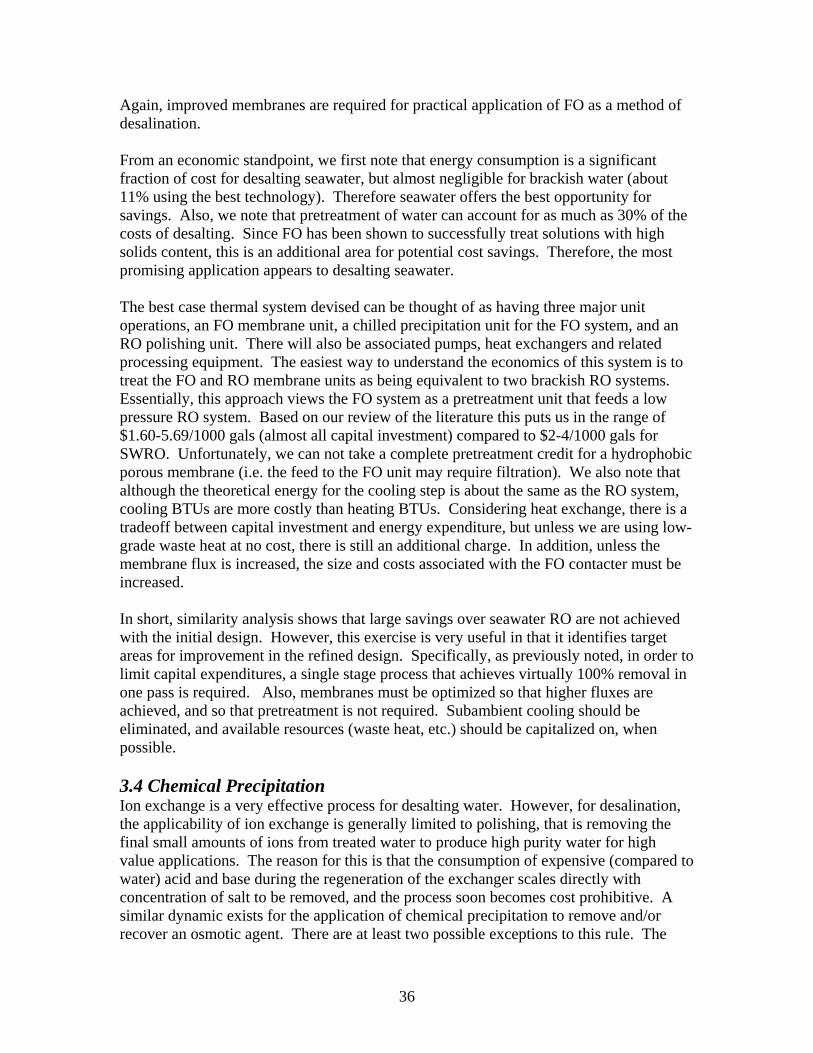
36

Again, improved membranes are required for practical application of FO as a method of desalination. From an economic standpoint, we first note that energy consumption is a significant fraction of cost for desalting seawater, but almost negligible for brackish water (about 11% using the best technology). Therefore seawater offers the best opportunity for savings. Also, we note that pretreatment of water can account for as much as 30% of the costs of desalting. Since FO has been shown to successfully treat solutions with high solids content, this is an additional area for potential cost savings. Therefore, the most promising application appears to desalting seawater. The best case thermal system devised can be thought of as having three major unit operations, an FO membrane unit, a chilled precipitation unit for the FO system, and an RO polishing unit. There will also be associated pumps, heat exchangers and related processing equipment. The easiest way to understand the economics of this system is to treat the FO and RO membrane units as being equivalent to two brackish RO systems. Essentially, this approach views the FO system as a pretreatment unit that feeds a low pressure RO system. Based on our review of the literature this puts us in the range of $1.60-5.69/1000 gals (almost all capital investment) compared to $2-4/1000 gals for SWRO. Unfortunately, we can not take a complete pretreatment credit for a hydrophobic porous membrane (i.e. the feed to the FO unit may require filtration). We also note that although the theoretical energy for the cooling step is about the same as the RO system, cooling BTUs are more costly than heating BTUs. Considering heat exchange, there is a tradeoff between capital investment and energy expenditure, but unless we are using low-grade waste heat at no cost, there is still an additional charge. In addition, unless the membrane flux is increased, the size and costs associated with the FO contacter must be increased. In short, similarity analysis shows that large savings over seawater RO are not achieved with the initial design. However, this exercise is very useful in that it identifies target areas for improvement in the refined design. Specifically, as previously noted, in order to limit capital expenditures, a single stage process that achieves virtually 100% removal in one pass is required. Also, membranes must be optimized so that higher fluxes are achieved, and so that pretreatment is not required. Subambient cooling should be eliminated, and available resources (waste heat, etc.) should be capitalized on, when possible. 3.4 Chemical Precipitation Ion exchange is a very effective process for desalting water. However, for desalination, the applicability of ion exchange is generally limited to polishing, that is removing the final small amounts of ions from treated water to produce high purity water for high value applications. The reason for this is that the consumption of expensive (compared to water) acid and base during the regeneration of the exchanger scales directly with concentration of salt to be removed, and the process soon becomes cost prohibitive. A similar dynamic exists for the application of chemical precipitation to remove and/or recover an osmotic agent. There are at least two possible exceptions to this rule. The

37

first would be an example where the resulting precipitate has market value. The second would be a case wherein the reaction resulting in precipitation is readily reversible, for example by thermal treatment. Figure 20 gives an example of the first case with H2SO4 being used as the osmotic agent. The addition of Ca(OH)2 to the spent osmotic solution precipitates gypsum (CaSO4). The figure shows that the value of gypsum helps to

offset the cost of the reagents, but not to the extent to make it

viable [61]. In fact, it is clear that the viability of this approach is limited to cases wherein the value of the product nearly meets or exceeds the value of the reagent. In other words, this approach will only be viable in the unlikely case that the precipitated salt is more valuable than the parent acid and base. An exploration of the second approach is discussed in the following section 3.5. 3.5 Salts of Carboxylic Acids and Carbon Dioxide In an earlier project to develop a process for lignin depolymerization, the possibility of neutralizing and precipitating reaction products from a basic solution through the addition of CO2 was considered [62]. It was thought that this approach might also be applicable to FO. Several examples of this approach are known in the literature, including processes to recover metals from aqueous solution [63], casein from milk [64,65], and soy protein from soy meal extract [66]. In our case, many of the reaction products from lignin depolymerization were phenolic in nature. Many phenols and related compounds lack sufficient solubility and/or have toxicity concerns that rule out their use for this application. However, investigating the solubility of weak acid compounds led us to the pharmaceutical literature wherein the solubility of medicinal agents is and the pH dependence of that solubility is an important consideration [67]. Figure 21 is a generalization of the relationship between solubility and pH for many weakly acidic compounds [67-70]. At low pH the acid is in protonated form and is therefore has a low intrinsic solubility (SN). As the pH is increased beyond the pKa, the acid dissociates into the more soluble form. Solubility then increases with pH until a maximum value is reached. Mathematically the generalization can be expressed as follows:

pH < pHMax: ST=SN(1+10 pH-pKa) pH > pHMax: ST=SMax

Weakly basic compounds display similar, but opposite behavior and therefore would likely be made more soluble by the addition of CO2.

NaCl concentration (ppm)

0 10000 20000 30000 40000

Rea

gent

cos

t ($/

1000

gal

)

0

5

10

15

20

No gypsum credit$10/ton gypsum credit$30/ton gypsum credit

Figure 20. Cost of desalination via gypsum precipitation from H2SO4 @ $49/ton and Ca(OH)2 @ $75/ton.

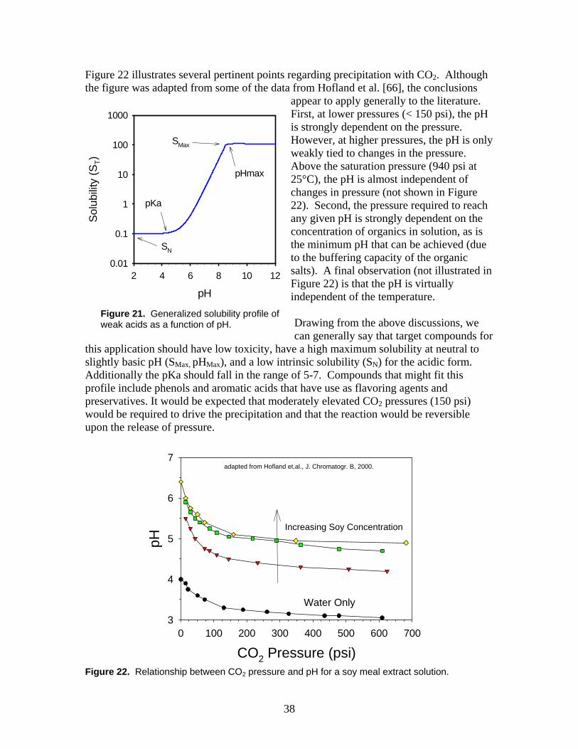
38

Figure 22 illustrates several pertinent points regarding precipitation with CO2. Although the figure was adapted from some of the data from Hofland et al. [66], the conclusions

appear to apply generally to the literature. First, at lower pressures (< 150 psi), the pH is strongly dependent on the pressure. However, at higher pressures, the pH is only weakly tied to changes in the pressure. Above the saturation pressure (940 psi at 25°C), the pH is almost independent of changes in pressure (not shown in Figure 22). Second, the pressure required to reach any given pH is strongly dependent on the concentration of organics in solution, as is the minimum pH that can be achieved (due to the buffering capacity of the organic salts). A final observation (not illustrated in Figure 22) is that the pH is virtually independent of the temperature. Drawing from the above discussions, we can generally say that target compounds for

this application should have low toxicity, have a high maximum solubility at neutral to slightly basic pH (SMax, pHMax), and a low intrinsic solubility (SN) for the acidic form. Additionally the pKa should fall in the range of 5-7. Compounds that might fit this profile include phenols and aromatic acids that have use as flavoring agents and preservatives. It would be expected that moderately elevated CO2 pressures (150 psi) would be required to drive the precipitation and that the reaction would be reversible upon the release of pressure.

CO2 Pressure (psi)0 100 200 300 400 500 600 700

pH

3

4

5

6

7

Water Only

Increasing Soy Concentration

adapted from Hofland et.al., J. Chromatogr. B, 2000.

Figure 22. Relationship between CO2 pressure and pH for a soy meal extract solution.

pH2 4 6 8 10 12

Sol

ubilit

y (S

T)

0.01

0.1

1

10

100

1000

pKa

pHmax

SN

SMax

Figure 21. Generalized solubility profile of weak acids as a function of pH.

39

Initially, three organic acids, salicylic acid, benzoic acid, and 4-hydroxybenzoic acid, were identified as potential candidates and lithium salts of these compounds were purchased for evaluation. Beginning from concentrations of 10 wt% salts, we were able to reduce concentrations over orders of magnitude by the addition of HCl (Figure 23). The lines in the figure represent the pKa values of the different acids. The inset figure illustrates pH adjustment of a Li-4-hydroxybenzoate solution through the addition of

CO2. Unfortunately we were unable to gauge the degree of precipitation induced by the CO2 overpressure with the equipment available as we were unable to filter the solution under pressure or extract a representative liquid sample. However, the results suggest that continuous or step removal of precipitate removal of precipitate would be required to overcome the buffering effect of the solution and achieve the highest levels of precipitation. Although the approach appears to have promise, the use of lithium salts is clearly unacceptable. First, the carbonate and bicarbonate salts of lithium are fairly soluble. Second, lithium carbonate is a drug used to treat mental disorders and as such should be avoided for this application. Magnesium and calcium salts are safer and less soluble alternatives. Regrettably,

they also tend to have limited maximum solubilities. Table 9 below lists several magnesium and calcium carboxylate salts and their respective solubilities measured in our laboratories. The salt solutions were prepared by mixing excess amounts of the carboxylic acid with a stoichiometric ratio of either calcium carbonate or magnesium carbonate in water at 65 °C. Note that this is the reverse of the proposed precipitation reaction and that it is a necessary step in the recovery and recycle process. The solubilities were determined by titrating a syringe filtered (0.45µ) sample with 1.0 N or 0.1 N HCl using a Mettler DL 70ES Titrator. Additionally, for each solubility test, the initial pH and the pH at equivalence point (pKa) was recorded. Of the salts evaluated only the salicylates (salicylic acid is 2-hydroxybenzoic acid) have significant solubilities. Of the two, magnesium has the higher solubility and the lower

pH

2 3 4 5 6 7 8 9

Con

cent

ratio

n (%

)

0.01

0.1

1

10

100Li SalicylateLi BenzoateLi 4-hydroxybenzoate

pKa

CO2 Pressure

0 50 100 150 200 250 300

pH

5.5

6.0

6.5

7.0

7.5

8.0

Figure 23 Solubility and pKa of several aromatic acid salts. Inset: pH as a function of CO2 pressure. Inset: pH as a function of CO2 pressure.

40

molecular weight (370.6 g/mol). The calculated osmotic pressure for a saturated magnesium salicylate solution at 65 °C is 44 atm. Our previous results suggest that this would yield a relatively low flux. The low pKa of the salicylic acid is also a concern for neutralization via CO2 addition. Table 9. Solubilities of select calcium and magnesium carboxylate salts. Carboxylate Salt Initial pH Equivalence pt. pH

(pKa) Solubility (wt. %)

Calcium Salicylate 3.7 2.3 18.3 Magnesium Salicylate 3.99 2.09 19.5 Calcium Isophthalate 5.4 3.2 2.3 Magnesium Isophthalate 5.1 3.5 6.3 Calcium 4-Methoxysalicylate

4.5 3.1 5.1

Magnesium 4-Methoxysalicylate

4.4 3.1 2.5

Calcium 5-Hydroxyisophthalate

See note 1

Magnesium 5-Hydroxyisophthalate

See note 1

Calcium 3,5-Dihydroxybenzoate

See note 2

Magnesium 3,5-Dihydroxybenzoate

See note 2

Calcium 4-Hydroxybenzoate

4.1 2.0 5.1

Magnesium 4-Hydroxybenzoate

4.4 2.0 6.3

Calcium Toluate 4.6 2.0 1.5 Magnesium Toluate 4.7 2.1 1.6 Notes: 1 – Apparent polymerization of the organic upon HCl addition. 2 - Carboxylic acid form was soluble but salt form was insoluble. As an interesting aside, 3.,5-dihydroxybenzoic acid was found to be soluble but insoluble as the salt form for either calcium or magnesium. Further tests were done to evaluate the solubility of this acid at various temperatures using a gravimetric method. Samples of saturated solutions of 3,5-dihydroxybenzoic acid were collected and filtered at various temperatures and then weighed. The samples were allowed to air dry at room temperature, were further dried at 100 °C for 12 hours, and the residues were then weighed. The results are shown in Table 10 along with calculated values for the osmotic pressure. The results are interesting in that the solubility is high at reasonable temperatures, is a strong function of temperature, and is relatively low at ambient temperatures. There is little change in solubility upon cooling to subambient temperatures. These properties make it of some interest for our originally proposed design. From a membrane point of view, the acidic pH is also attractive. Of course the same limitations apply in that 3,5-dihydroxybenzoic acid can not be fully removed with a

41

single precipitation step. In this case however there are options other than RO for removing the remaining organic from solution such as adsorption on activated carbon (provide it can be efficiently regenerated with low grade steam). A related possibility is reaction with or adsorption on Ca(OH)2 followed by steam regeneration of both acid and base. This method has been demonstrated for recovering phenols, but to our knowledge not for acids [71]. A similar process for phenols has been reported wherein the phenols are recovered from the phenolate salts by reaction with CO2 [72]. Overall, however, the additional capital and energy expenditures required for this approach would seem to make it an unattractive alternative to RO.

Table 10. Solubility as function of temperature for 3-5-dihyroxybenzoic acid. Temperature ( C ) Solubility (wt. %) Osmotic Pressure (atm)

75 38.5 143 60 27.8 99 50 22.5 77 45 16.5 56 31 11.1 36 23 3.9 12 15 4.5 14 10 4.7 14 3 3.3 9.6

In conclusion we were unable to identify an osmotic agent of sufficient solubility in an appropriate salt form to capitalize on this revised approach. It is possible that others may have more success in doing so. 4. The Cost of Using FO as a Pretreatment Technology One of the possible applications of FO is that of a pretreatment technology to condition particularly difficult streams (e.g. with high fouling or scaling potential) for conventional or high recovery RO. An initial cost estimate for this application was developed using the Water Treatment Estimation Routine (WaTER) developed by the United States Department of the Interior, Bureau of Reclamation. To provide the most meaningful estimate, a comparison of the cost for treating brackish water with and without a FO pretreatment step was made. WaTER is an Excel® spreadsheet program developed to provide estimates of water treatment plant costs. The program was adapted from the U.S EPA 1979 report, Estimating Water Treatment Costs, Vol.2, Cost Curves Applicable to 200 mgd Treatment Plants [73]. The program considers production capacity and a water analysis and uses a set of generalizations to specify equipment for a particular water treatment process. System sizing calculations are based on user inputs. The Cost output of the program is given in current dollars derived either from Engineering News Record (ENR) or Bureau of labor Statistics (BLS) cost indices that are entered by the user. Estimates of annual unit water cost are based on annual operation and maintenance costs and the amortized capital recovery cost for a given interest rate. Further information on the WaTER

42

program can be obtained from the Bureau of Reclamation, Water Desalination Research & Development Program Report No. 43. Previous studies have shown it is difficult to generalize a definitive cost for brackish water reverse osmosis. The costs for BWRO compiled by Miller [5] range from $0.70 to $2.65 per 1000 gallons of treated brackish water. Installed costs of BWRO reported by Henthorne based on contracts placed during 2001 to 2003 ranged from $680 - $1500/kgal/day of installed product capacity [74]. The range in costs is a function of the variability in the size of the systems and the additional facilities required for pretreatment, concentrate disposal, pipelines, annual maintenance and operating requirements, etc. The variability in costs of RO systems is much debated subject regarding what is the true cost of desalting water by RO processes. The approach taken here for cost evaluation of FO and BWRO was to assume best case conditions. Specifically, it was assumed that the water being treated had no unusual pretreatment requirements and would not create difficult maintenance problems. The brackish water specifications, given below, were based on water from the Tularosa Basin in southeast New Mexico. The cost evaluation assumed a 5 mgd plant operating at 95% availability for 20 years at 6% interest. A 5 mgd plant was used for evaluating costs since capital cost of RO plants are fairly flat for capacities of 5 mgd or greater [75]. Blending of feed water was not considered nor was waste or concentrate disposal as it was assumed to be similar for both cases. Table 11. Specifications of feed water for cost evaluations Total Dissolved Solids, TDS 3070 mg/L High Sulfate concentration 1100 mg/L Bicarbonate Alkalinity 125 mg/L Low silica concentration 12 mg/L Calcium concentration 110 mg/L Magnesium 80 mg/L Anion/Cation equivalence 0.0479 eq/L Consider the BWRO system first. The calculations assumed a system capable of 95% recovery of the feed. To achieve this high recovery, the system was setup with two two-stages. The first stage was a BWRO system operated at 80% recovery and 99.5% salt rejection. The second stage was a seawater RO system, operating at 75% recovery and 99.1% salt rejection. Achieving an overall 95% recovery is an optimistic assumption; however, it is not unreasonable since 80% recovery BWRO is not unusual for an efficiently operated plant with no abnormal maintenance problems. The 75% water recovery SWRO may seem overly optimistic. However, the feed to the second stage is not seawater, but brackish water concentrated to only about 15,000 mg/L, well below the 35,000 mg/L that is typical for a SWRO system. Thus, 75% recovery is feasible as a best case condition for the second stage. It was further assumed that acidification and antiscalant addition were necessary and sufficient for control of carbonate and silica scaling. It was assumed that the sulfate did not present an additional scaling problem. No post treatment, e.g. alkalinity adjustment, was considered in the cost analysis. The

43

membranes for the system were assumed to be Dow FilmTec RO membranes. The first stage was outfitted with 8 inch diameter BW30-400 membranes, with an optimum flux of 25 gal/ft2/day (42.4 l/m2/hr). The second stage was outfitted with 8 inch diameter SW30-8040 membranes with an optimum flux of 15 gal/ft2/day (25.5 l/m2/hr). The flux rates are those provided by the manufacturer for new membranes. It was assumed that the membranes would be replaced every 3 years. Given these inputs, stage 1 of the system incorporated 414 membranes placed in 69 pressure vessels, and the stage 2 units consisted of 180 membranes placed in 30 pressure vessels. The key cost elements for the BWRO system are:

• Total capital cost of about $5 million. • Annual O&M cost of $1.5 million/yr. • Annualized capital cost (capital recovery @ 6% over 20 years) of $0.4 million. • Total annual operating cost of $1.9 million/yr or $1.16/kgal.

Note that the water cost is at the low end of, but consistent with, values reported in the literature. Now consider a similar system with a single stage FO add-on for pretreatment. Again, consider a system capable of 95% recovery of the feed. For the calculations, the osmotic agent was assumed to be sodium chloride, NaCl. The FO pretreatment unit would dewater the incoming brackish water by a concentration factor of twenty. That is, the brackish water must be concentrated from its initial TDS of 3070 mg/L to 61,400 mg/L. The diluted osmotic agent would be treated by conventional SWRO to recover the water transferred into the osmotic agent and concentrate the osmotic agent back to its initial concentration. It is assumed that scaling is not an issue in the FO unit. Of course, with NaCl as the osmotic agent, it is also not an issue for the SWRO unit. For the calculations, a de-rated FilmTec RO membrane was assumed for the FO system. That is, it was assumed that the flux across the FO membrane was 6 gal/ft2/day (10 l/m2/hr). As discussed in previous sections of this report, a specially tailored FO membrane might yield better fluxes, but for existing RO membranes, this appears to be a reasonably optimistic assumption (see section 2.2). Data reported for FilmTec30 membranes [76] for net driving pressure, (operating pressure minus the osmotic pressure differential across the membrane) was used to estimate osmotic driving force required to achieve this flux. A driving force of 203 psi was reported to give a flux of 20 gal/ft2/day through a FilmTec30 membrane. Assuming a linear relationship between driving force and flux, approximately 61 psi of osmotic pressure differential would be required to achieve the 6 gallons/ft2/day. Estimating the osmotic pressure of the brackish water from the TDS as being equivalent to 3070 mg/L NaCl, an osmotic agent concentration of at least 8020 mg/L (or a difference of at least 4950 mg/L) would be required to produce a net driving pressure of over 61 psi. Using these assumptions, the FO portion of the system would consist of 2088 FilmTecBW30 membranes placed in 348 pressure vessels at a capital cost of about $5.6 million. The annual operating cost of the FO system would be about $0.60/kgal of produced water. If one assumes that a constant driving force across the membrane of 61

44

psi (or 4950 ppm NaCl) is sufficient, then cost of the system to recover water and concentrate the osmotic agent closely mirrors that of the BWRO system described above, with the exception that that the acid addition and antiscalant are no longer required. The annualized cost of these pretreatments is about $0.06/kgal. Therefore, the cost of pretreating this stream via FO is $0.54/kgal. This relatively high cost results from the low value assumed for flux across the membrane. If the FO flux is increased 70% to10 gal/ft2/day (17 liters/m2/hr), the unit water costs drops by only 30% to about $0.38/kgal. It is important to note that the above calculations assume a constant and relatively low osmotic pressure differential of 61 psi (or only 4950 mg/L NaCl). Given the likelihood of concentration polarization and other deleterious effects, this is a very optimistic assumption. If a greater driving force is required to achieve the desired flux, there will be a significant price to pay in the concentrating the osmotic agent. For example, consider a case where the flows in the FO system are balanced such the concentration ratio, rather than the concentration difference, is kept constant. In this case the osmotic agent would be concentrated to 160,400 mg/L, rather than the previous 66,350 mg/L. This process would now require a two-stage SWRO system. Our model included a first stage operating at 80% water recovery and flux of 15 gal/ft2/day, and a second stage operating at 75% water recovery and a flux of 15 gal/ft2/day. These are optimistic water recovery conditions for a SWRO system; but a reasonable best case condition for a clean solution of osmotic agent. Given these inputs, the first stage of the osmotic agent concentration system consisted of 936 FilmTecSW30 membranes placed in 156 pressure vessels operating at a pressure of 498 psi, producing 4.2 mgd of water and the second stage RO system consisted of 180 FilmTecSW30 membranes placed in 30 pressure vessels operating at a pressure of 1600 psi, producing 0.8 mgd of water. The key cost elements for this system are:

• Annual operating cost of the first stage RO is about $1.3/kgal of produced water and a capital cost of about $5.3 million.

• Annual operating cost of the second stage RO is about $3.10/kgal of produced water at a capital cost of about $1.4 million.

• Total operating cost of $1.62/kgal of produced water at a total capital cost of $6.7 million.

This is $0.52/kgal above the $1.10/kgal required for the constant concentration differential case, bringing the total cost resulting from the FO pretreatment in this case to $1.06/kgal. This calculation is a bit misleading as a flux increase in the FO might result from the increased concentration of the osmotic agent. However, our calculations suggest that it is unlikely that gains in flux will be able to fully offset the cost of increasing the concentration of the osmotic agent. 5. Late Breaking News During the course of this project/writing of this report there were several developments deserving of mention. The first was the awarding of a U.S. patent to R.L. McGinnis for a forward osmosis process for desalination [77]. The McGinnis process tackles the problem of incomplete removal/precipitation of the primary osmotic agent (in this case KNO3) by thermal means by passing the cooled KNO3 stream to a secondary FO

45

contactor in which dissolved SO2 (apparently under pressure) is used as the osmotic agent. The SO2 is thermally stripped to recover water. It was proposed that a third osmotic agent whose presence is desirable for the final water application, e.g. NaF for drinking water or NH4NO3 for agricultural purposes, be used for a third and final polishing step. Overall, the approach outlined in the patent is quite clever. But, as discussed above, processes such as this one that are significantly more complex than RO are very unlikely to be economical. More recently McCutcheon, McGinnis and Elimelech coauthored two papers describing a FO process that utilizes ammonium bicarbonate, (NH4)HCO3, or ammonium carbamate, H2NCO2NH4, as the osmotic agent [78,79]. In this case, the (NH4)HCO3 is decomposed into CO2 and NH3 by low grade heat and is stripped from solution. The two journal articles concentrate on the FO step, and although the data is promising, the need for improved or optimized membranes is evident. Still, from an overall process standpoint, the design and performance (capital and operating costs) of the distillation column required to strip and recover the osmotic agent and which is not discussed in the present literature will likely be the determining factor in the viability of this process. The limits for ammonia in drinking water are particularly stringent at 2 mg/L. Another alterative osmotic agent that has recently been publicized is magnetoferritin. Magnetoferritin is essentially a spherical shell comprised of protein molecules with a magnetic core of iron oxide or other metals. It has been proposed that magnetoferritin could be used as an osmotic agent and then recovered with a magnetic field. There has been a fair amount of publicity of this approach and claims of near commercialization, much of which can be found on the internet [80]; however, to date we have been unable to locate any technical information regarding actual testing of this approach. It is unclear at this point what osmotic pressures may be attainable with magnetoferritin and to what streams the technology might be applicable. There has been a recent publication regarding a related approach wherein the magnetoferritin is being modified to selectively bind ions for removal from solution [81]. Another recent pair of articles reported the application of FO as a pretreatment for RO [82,83]. In addition these articles report overlaying FO membranes with microporous hydrophobic membranes to, in effect, form a single membrane that carries out both FO and osmotic distillation processes. This has the advantage of protecting the hydrophobic membrane from surfactants, for example, while achieving the separation of low molecular weight compounds such as urea that are capable of permeating the FO membrane. The application of interest in this case was the reclamation of wastewater for reuse, for example in space travel. Finally, there is a recent report that compares the performance of two conventional RO membranes to a FO membrane for several osmotic agents including ammonium bicarbonate, glucose and fructose [84].

46

6. Concluding Remarks and Recommendations Fresh, potable water is an essential human need. The promise of forward osmosis is that it will provide a low cost method for meeting that need. However, the decades of developing and improving RO have set the bar very high for would-be commercial desalination technologies. In its current embodiments, FO will not dislodge RO as the most favored desalination technology, particularly for routine waters. However, a future role for FO is not out of the question. The ability to treat waters with high solids content or fouling potential is particularly attractive. Although our analysis indicates that FO is not cost effective as a pretreatment for conventional BWRO, water scarcity will likely drive societies to recover potable water from increasingly marginal resources, for example gray water and then sewage. In this context, FO, perhaps in a membrane bioreactor arrangement, may be an attractive pretreatment alternative. Water scarcity, as well as the management and cost of brine disposal, will also likely drive desalination ever closer to the zero-discharge limit. More than 30 years ago, Loeb and Bloch recognized the potential for applying osmotic agents to assist in dewatering brines [85]. Although membrane improvements and pressure recovery devices have made ideas such as concentrate return RO less relevant, the issues of precipitation, fouling, and scaling in high recovery operations remain. FO offers a potentially elegant solution to these operating difficulties, provided the value of the recovered water or expense of brine disposal justifies the added cost. Moving forward, work remains before FO can fulfill its promise. The creative application of FO to new and difficult problems and demonstration of those applications will be necessary to validate the advantages of FO in treating challenging waters, as well as to fully characterize the limits and economics of the process. Continued improvement and optimization of membranes will be a necessary and critical part of this development. Finally, the identification of optimal osmotic agents for different scenarios may also be important. Although simple agents such as NaCl and an RO concentrating step may well prove to be ideal for avoiding scaling in high recovery applications, it is clear that the space of potential agents and recovery processes has not been fully explored. For example, to our knowledge anti-solvent crystallization or extractive crystallization [86] has not been discussed in the context of FO. 7. References

1. R. Engelman, R.P. Cincotta, B. Dye, T. Gardner-Outlaw, J. Wisnewski “People in the Balance: Population and Natural Resources at the Turn of the Millennium” Population Action International, Washington, D.C. (2000). 2. G.F. Leitner, Int. Desalination and Water Reuse Quart. 7 (1998) 10. 3. Maude Barlow and Tony Clark in Blue Gold, New Press, New York, 2002. 4. J. Rothfeder in Every Drop for Sale, Tarcher/Putnam, New York, 2001. 5. J.E. Miller, “Review of Water Resources and Desalination Technologies” Sandia National Laboratories Report, SAND2003-0800, February 2003. 6. O.K. Buros, “The ABCs of Desalting, Second Ed.” International Desalination Association, Topsfield, Mass, 2000. 7. R.V. Wahlgren, Wat. Res. 35 (2001) 1.

47

8. See for example L.J. Hauge, Desalination 102 (1995) 219. 9. G.G. Pique, Water Conditioning and Purification, July 2000. 10. K.S. Spiegler and Y.M. El-Sayed, A Desalination Primer, Balaban Desalination Publications, Santa Maria Imbaro, Italy (1994). 11. K.S. Spiegler, Y.M. El-Sayed, Desalination 134 (2001) 109 and Y.M. El-Sayed Desalination 134 (2001) 129. 12. Standards are available at www.epa.gov/safewater/consumer/2ndstandards.html 13. G.F. Leitner, Desalination and Water Reuse Quarterly 5 (1995) 24. 14. G.A. Pittner in Reverse Osmosis, Z. Amjad, ed. Chapman Hall, New York (1993). 15. R. Semiat, Water International, Vol. 25, 54, (2000). 16. R. Semiat, Water International 25 (2000) 54. 17. H.T. El-Dessouky, H.M. Ettouney, Y. Al-Roumi, Chemical Engineering Journal 73 (1999) 173. 18. K. Popper, R.L. Merson, W.M. Camirand, Science 159 (1968) 1364. 19. J.F. Osterle and W.W. Feng, ASME Paper (1974) 74-WA/Ener-1. 20. R.E. Kravath and J.A. Davis, Desalination 16 (1975) 151. 21. C.D. Moody and J.O. Kessler, Desalination 18 (1976) 283. 22. C.D. Moody and J.O. Kessler, Desalination 18 (1976) 297. 23. See for example, M. Wong and R.J. Winger, Food Australia 51 (1999) 200. 24. F. Vaillant, E. Jeanton, M. Dornier, G.M. O’Brien, M. Reynes, M. Decloux, J. Food Engineering 47 (2001) 195. 25. R. Salter, Osmotek, personal communication. 26. For examples of these types of applications see D.O. Kuethe, D.C. Augenstein, J.D. Gresser, D.L. Wise, J. Control. Release, 18 (1992) 159; E.L. Michelson, Clin. Cardiol. 14 (1991) 947; J.M. Cornejo Bravo, and R.A. Siegel, Poly. Mater. Sci. Eng. Proc. ACS Div. Polym. Mater. Sci. Eng. 66 (1992) 230; and Z.J. Twardowski, K.D. Nolph, R. Khanna, H. Hain, H. Moore, T.J. McGary, Mat. Res. Symp. Proc. 55 (1986) 319. 27. See for example S. Loeb, F. van Hessen, J. Levi, M. Ventura, 11th Intersociety Energy Conversion Engineering Conference, 1976, Nevada, or A. Seppala, M.J. Lampinen, W. Kotiaho, Int. J. Energy Res. 25 (2001) 1359. 28. S. Loeb, Desalination 141 (2001) 85. 29. M.S.M. Lefebvre, US Patent 4,781,837 (1988). 30. R.A. Johnson, R.H. Valks, and M.S. Lefebvre, Australian Journal of Biotechnology 3 (1989) 206. 31. J. Sheng, R.A. Johnson, M.S. Lefebvre, Desalination 80 (1991) 113. 32. J.I. Mengual, J. M. Ortiz de Zarate, L. Pena, A. Velazquez, J. Membrane Sci. 82 (1993) 129. 33. J. Sheng, Australian Chem. Eng. Conf. 3 (1993) 429. 34. R.J. Durham and M.H. Nguyen, J. Membrane Sci. 87 (1994) 181. 35. W. Kunz, A. Benhabiles, R. Ben-Aim, J. Membrane Sci. 121 (1996) 25. 36. C. Gostoli, J. Membrane Sci. 163 (1999) 75. 37. A.F.G. Bailey, A.M. Barbe, P.A. Hogan, R.A. Johnson, J. Sheng, J. Membrane Sci. 164 (2000) 195. 38. F. Lagana, G. Barbieri, E. Drioli, J. Membrane Sci. 166 (2000) 1.

48

39. F. Vaillant, E. Jeanton, M. Dornier, G.M. O’Brien, M. Reynes, M. Decloux, J. Food Engineering 47 (2001) 195. 40. K.W. Lawson and D.R. Lloyd, J. Membr. Sci. 124 (1997) 1. 41. M.P. Godino, L. Pena, J.M. Ortiz de Zarate, J.I. Mengual, Sep. Sci. Technol., 30 (1995) 993. 42. K.B. Petrotos, H.N. Lazarides, J. Food Engineering 49 (2001) 201. 43. K. Popper, W.M. Camarind, F. Nury, W.L. Stanley, Food Engineering 38 (1966) 102. 44. K.B. Petrotos, P.C. Quantick, H. Petropakis, J. Membrane Sci. 150 (1998) 99. 45. K.B. Petrotos, P.C. Quantick, H. Petropakis, J. Membrane Sci. 160 (1999) 171. 46. E.G. Beaudry, K.A. Lampi, Food Technology 44 (1990) 121. 47. E.G. Beaudry, K.A. Lampi, Fluessiges Obst 57 (1990) 652 and 663. 48. R.E. Wrolstad, M.R. McDaniel, R.W. Durst, N. Micheals, K.A. Lampi, E.G. Beaudry, J. Food Sci. 58 (1993) 633. 49. J.R. Herron, E.G. Beaudry, C.E. Jochums, L.E. Medina, US Patent 5,281,430 (1994). 50. K. Pitzer, J. Phys. Chem. 77 (1973) 268; K.S. Pitzer, G. Mayorga, J. Phys. Chem 77 (1973) 2300; K.S. Pitzer, G. Mayorga, J. Solution Chem. 3 (1974) 539; K.S. Pitzer J.J. Kim, J. Am. Chem. Soc. 96 (1974) 5701; K.S. Pitzer J. Solution Chem. 4 (1975) 249; and K.S. Pitzer, L.F. Silvester J. Solution Chem. 5 (1976) 269. 51. D.A. Amos, J.H. Markels, S. Lynn, C.J. Radke, J. Phys. Chem. B 1998, 102, 2739. 52. See for example R.N.M.R. van Gelder, K.J. Roberts, J. Chambers, T. Instone, J. Crystal Growth 166 (1996) 189; or M. Ambrosi, P. Lo Nostro, L. Frantoni, L. Dei, B.W. Ninham, S. Palma, R.H. Manzo, D. Allemandi, P. Baglioni, Phys. Chem. Chem. Phys. 6 (2004) 1401. 53. J.M.C. Bravo, R.A. Siegel “Studies of Precipitating and Soluble Hydrophobic Polyelectrolytes” Polymeric Materials Science and Engineering 66 (1992) 230. 54. A number of extensive references are available. See for example H. Stephen and T. Stephen, Solubilities of Inorganic Compounds, Vol.1 – Binary Systems, Part 1. 55. CRC Handbook of Chemistry and Physics, 61st Ed., CRC Press, Boca Raton FL, (1980). 56. F. Smagghe, J. Mourgues, J.L. Escudier, T. Conte, J. Molinier, C. Malmary, Bioresource Technology 39 (1992) 185. 57. P.A. Hogan, R. Philip Canning, P.A. Peterson, R.A. Johnson, A.S. Michaels, Chemical Engineering Progress July 1998, 49. 58. L.R. Evans and J.E. Miller “Sweeping Gas Membrane Desalination Using Commercial Hydrophobic Hollow Fiber Membranes” Sandia National Laboratories Report SAND2002-0138, January 2002. 59. Peter Eriksson, personal communication with Lindsey Evans. 60. Ed Beaudry, personal communication with Lindsey Evans. 61. For a brief summary of gypsum synthesis consult the archives at www.wconline.com. 62. J. E. Miller, L.R. Evans, J. Mudd, and K. Brown “Batch Microreactor Studies of Lignin Depolymerization by Bases: 2. Aqueous Solvents” Sandia National Laboratories Report, SAND2002-1318, May 2002.

49

63. Enick, R.M.; Beckman, E.J.; Shi, C.; Xu, J.; Chordia, L. “Remediation of Metal-Bearing Aqueous Waste Streams via Direct Carbonation” Energy & Fuels 2001, 15, 256. 64. Tomasula, P.M.; Craig, J.C.; Boswell, R.T. “A Continuous Process for Casein Production Using High-pressure Carbon Dioxide” J. Food Eng. 1997, 33, 405. 65. Hofland, G.W.; van Es, M.; van der Wielen, L.A.M.; Witkamp, G.J. “Isoelectric Precipitation of Casein Using High-Pressure CO2” Ind. Eng. Chem. Res. 1999, 38, 4919. 66. Hofland, G.W.; de Rijke, A.; Thiering, R.; van der Wielen, L.; Witkamp, G.J. “Isoelectric Precipitation of a Soybean Protein Using Carbon Dioxide as a Volatile Acid” J. Chromatogr. B 2000, 743, 357. 67. Chowhan, Z.T. “pH-Solubility Profiles of Organic Carboxylic Acids and Their Salts,” J. of Pharmaceutical Sciences, 1978, 63, 1257-1260. 68. W.H. Streng, S.K. HIS, P.E. Helms, H.G.H. Tan “General Treatment of pH-Solubility Profiles of Weak Acids and Bases and the Effects of Different Acids on the Solubility of a Weak Base” J. Pharm. Sci. 73 (1984) 1679. 69. W.H. Streng “The Gibbs Constant and pH Solubility Profiles” Intl. J. of Pharmaceutics 186 (1999) 137. 70. A. Avdeef “pH-metric Solubility. 1. Solubility-pH profiles from Bjerrum Plots. Gibbs Buffer and pKa in the Solid State” Pharm. Pharmacol. Commun. 4 (1998) 165. 71. C.G. Scouten and H. W. Dougherty “Organic Chemistry of Calcium. 3. Steam Stripping of Metal Phenoxide liberates Phenol and Regenerates the Metal Hydroxide” Ind. Eng. Chem. Res. 29 (1990) 1721. 72. P.K. Pahari and M.M. Sharma “Separation of Close-Boiling Substituted Phenols by Anhydrous Calcium Hydroxide and Recovery of Phenols from Calcium Phenoxide by Carbonation” Ind. Eng. Chem. Res. 31 (1992) 2040. 73. EPA-600/2-79-1626, August 1979. 74. L. Henthorne, “Cost of Current Membrane Technology” Water & Waste Tech Asis Conference, 2003. 75. Water Treatment Membrane Processes, Chapter 9, American Water Works Association Research Foundation, Lyonnaise des Eaux, Water Research Commission of South Africa, McGraw-Hill, (1996). 76. Zahid Amjad, “Membrane Technology, Water Chemistry, and Industrial Applications” Chapter 2, International Thomson Publishing, Chapman & Hall, 1993. 77. U.S. Patent 6,391,205 “Osmotic Desalination Process” (2002). 78. J.R. McCutcheon, R.L. McGinnis, M. Elimelech “A Novel Ammonia-Carbon Dioxide Forward (Direct) Osmosis Desalination Process” Desalination 174 (2005) 1. 79. J.R. McCutcheon, R.L. McGinnis, M. Elimelech “Desalination by Ammonia-Carbon Dioxide Forward Osmosis: Influence of Draw and Feed Solution Concentrations on Process Performance” J. Membr. Sci. 278 (2006) 114. 80. For examples see www.softmachines.org/wordpress/index.php?p=68; http://www.wired.com/news/technology/0,65287-0.html; http://ecofinance.blogware.com/blog/_archives/2005/11/9/1885306.html http://www.clubofamsterdam.com/content.asp?contentid=461 81. J. Duffield, I. Pascual, D. Bradbury, N. Ratcliffe, S. Bushart, G. Elder “The Development of Magnetic Molecules for the Selective Removal of Contaminants”

50

Proceedings - 10th International Conference on Environmental Remediation and Radioactive Waste Management, ICEM'05; 2005; v.2005, p.1812-1818. 82. T.Y. Cath, S. Gormly, E.G. Beaudry, M.T. Flynn, V.D. Adams, A.E. Childress “Membrane Contactor Processes for Wastewater Reclamation in Space. Part I. Direct Osmotic Concentration as Pretreatment for Reverse Osmosis” J. Membr. Sci. 257 (2005) 85. 83. T.Y. Cath, D. Adams, A.E. Childress “Membrane Contactor Processes for Wastewater Reclamation in Space. Part II. Combined Direct Osmosis, Osmotic Distillation, and Membrane Distillation for Treatment of Metabolic Wastewater” J. Membr. Sci. 257 (2005) 111. 84. H.W. Ng, W. Tang, W.S. Wong “Performance of Forward (Direct) Osmosis Process: Membrane Structure and Transport Phenomenon” Environ. Sci. Technol. 40 (2006) 2408. 85. See for example S. Loeb and M.R. Bloch “Countercurrent Flow Osmotic Processes for the Production of Solutions Having a High Osmotic Pressure” Desalination 13 (1973) 207. 86. The literature is rich in these topics. For recent examples see: M.S.H. Bader “Separation of Critical Radioactive and Non-radioactive Species from Aqueous Waste Streams” J. Hazardous Matls. B82 (2001) 139; T.G. Ziljema. R.M. Geertman, G.-J. Witkamp, G.M. van Rosmalem, J. de Graauw “Antisolvent crystallization as an Alternative to Evaporative Crystallization for the Production of Sodium Chloride” Ind. Eng. Chem. Res. 39 (2000) 1330; and A. Cartón, S. Bolado, M. Marcos "Liquid-Liquid Equilibria for Aqueous Solutions of Lithium Sulfate or Lithium Formate and Triethylamine or Diisopropylamine” J. Chem. Eng. Data 45 (2000) 260.

51

DISTRIBUTION:

10 MS 1349 James Miller, 1815 5 MS 1349 Lindsey Evans, 1815 1 MS 1349 Bill Hammetter, 1815 1 MS 0887 Justine Johannes 1810 1 MS 0887 Duane Dimos 1800 1 MS 0754 Patrick Brady, 6118 1 MS 0755 Mike Hightower, 6212 1 MS 0701 Peter Davies, 6100 1 MS 0701 John Merson, 6110 1 MS 1089 Fran Nimick, 6140 1 MS 0754 Tom Hinkebein, 6118 1 MS 0754 Richard Kottenstette, 6118 1 MS 0754 James Krumhansl, 6118 1 MS 0754 Thomas Mayer, 6118 1 MS 0754 Malcolm Siegel, 6118 1 MS 0754 Malynda Aragon, 6118 1 MS 0123 LDRD, Donna Chavez, 1011 2 MS 9018 Central Technical Files, 8944 2 MS 0899 Technical Library, 4536