Forward Guidance and the Exchange Rate

Jordi Galí ∗

February 2018(first draft: May 2017)

Abstract

I analyze the effectiveness of forward guidance policies in open economies, focusing onthe role played by the exchange rate in their transmission. An open economy version ofthe "forward guidance puzzle" is shown to emerge. In partial equilibrium, the effect onthe current exchange rate of an anticipated change in the interest rate does not declinewith the horizon of implementation. In general equilibrium, the size of the effect is largerthe longer is that horizon. Empirical evidence using U.S. and euro area data euro-dollarpoints to the presence of a forward guidance exchange rate puzzle: expectations of interestrate differentials in the near (distant) future have much larger (smaller) effects on theeuro-dollar exchange rate than is implied by the theory.

JEL Classification: E43, E58, F41,Keywords: forward guidance puzzle, uncovered interest rate parity, unconventional

monetary policies, open economy New Keynesian model.

∗CREI, Universitat Pompeu Fabra and Barcelona GSE. E-mail: jgali@crei.cat. I have benefited from com-ments by Jón Steinsson, Shogo Sakabe, Philippe Bacchetta, Wenxin Du, and Marty Eichenbaum.and participantsat seminars and conferences at CREI-UPF, Banco de España, SAEe 2017, Riksbank, Bocconi-Bank of Canada,ECB and U. of Edinburgh. I thank Philippe Andrade for help with the data, and Christian Hoynck, CristinaManea and Matthieu Soupre for excellent research assistance. I acknowledge financial support from the CERCAProgramme/Generalitat de Catalunya and the Severo Ochoa Programme for Centres of Excellence.

1 Introduction

The challenges posed by the global financial crisis to central bankers and the latter’s increasingreliance on unconventional monetary policies has triggered an explosion of theoretical andempirical research on the effectiveness of such policies, i.e. policies that seek to substitute forchanges in the short-term nominal rate —the instrument of monetary policy in normal times—when the latter attains its zero lower bound (ZLB). A prominent example of an unconventionalpolicy adopted by several central banks in recent years is given by forward guidance, i.e. theattempt to influence current macroeconomic outcomes by managing expectations about thefuture path of the policy rate once the ZLB is no longer binding.In the present paper I analyze the effectiveness of forward guidance policies in an open

economy, focusing on the role played by the exchange rate in their transmission. As I discussbelow, that transmission hinges to an important extent on the dependence of the exchangerate on the undiscounted sum of expected future interest rate differentials, as implied by thetheory. Importantly, that relation relies only a (relatively) weak assumption: the existence ateach point in time of some investors with access to both domestic and foreign bonds.In the first part of the paper I analyze the effects of forward guidance on the exchange

rate, under the assumption of constant prices (or, equivalently, when the induced effects of theinterest rates and the exchange rate on output and prices are ignored). In that environment,the combination of uncovered interest parity with the long run neutrality of monetary policyyields a strong implication: the impact on the current exchange rate of an announcement of afuture adjustment of the nominal rate is invariant to the timing of that adjustment.Next I turn to the analysis of forward guidance policies in general equilibrium, i.e. allowing

for feedback effects on output and prices, using a simple New Keynesian model of a smallopen economy. In general equilibrium, the size of the effect of forward guidance policies onthe exchange rate is shown to be larger the longer is the horizon of implementation of a givenadjustment in the nominal interest rate. A similar prediction applies to the effect on outputand inflation. Both results are closely connected to the findings in the closed economy literatureon the forward guidance puzzle, as discussed below.1

The same framework can be used to analyze the relation between the effectiveness of forwardguidance policies and openness. I start by showing a simple condition under which the size ofthe effects of forward guidance policies on the exchange rate and other macro variables isinvariant to the economy’s openness. When that condition does not apply, the sign of thatrelation between openness and the size of the effects of forward looking policies can no longerbe pinned down analytically. As an illustration, I show that under my baseline calibration theimpact of forward guidance on some variables (output, the nominal exchange rate) increaseswith the degree of openness, whereas the opposite is true for some other variables (e.g., the realexchange rate).Finally, I turn to the data, and provide some empirical evidence on the role of current and

expected future interest rate differentials as a source of exchange rate fluctuations. Using dataon euro-dollar exchange rate and market-based forecasts of interest rate differentials betweenthe U.S. and the euro area, I provide evidence suggesting that expectations of interest ratedifferentials in the near (distant) future have much larger (smaller) effects than is implied

1See Del Negro et al. (2015), and McKay et al. (2016, 2017), among others,

1

by the theory. I refer to the apparent disconnect between theory and empirics on this issueas the forward guidance exchange rate puzzle, and discuss why the solutions to the forwardguidance puzzle found in the closed economy literature are unlikely to apply in the presence ofan exchange rate channel.The remainder of the paper is organized a follows. Section 2 describes the related literature.

Section 3 discusses the effects of forward guidance on the exchange rate in a partial equilibriumframework. Section 4 revisits that analysis in general equilibrium, using a small open economyNew Keynesian model as a reference framework. Section 5 presents the empirical evidence.Section 6 summarizes and concludes.

2 Background: The Forward Guidance Puzzle

The effectiveness of forward guidance and its role in the design of the optimal monetary policyunder a binding ZLB was analyzed in Eggertsson and Woodford (2003) and Jung et al. (2005),using a standard New Keynesian model. Those papers emphasized the high effectiveness offorward guidance as a stabilizing instrument implied by the theory, at least under the maintainedassumption of credible commitment.More recently, the contributions of Carlstrom et al. (2015), Del Negro et al. (2015), and

McKay et al. (2016, 2017), among others, have traced the strong theoretical effectiveness offorward guidance to a "questionable" property of one of the key blocks of the New Keynesianmodel, the Euler equation, which in its conventional form implies that future interest rates arenot "discounted" when determining current consumption. Formally, the dynamic IS equation(DIS) of the New Keynesian Model can be solved forward and written as:

yt = − 1

σ

∞∑k=0

Et{rt+k}

where yt is (log) output and rt ≡ it−Et{πt+1} is the real interest rate. Thedenotes deviationsfrom steady state. Note that the predicted effect on output of a given anticipated change in thereal interest rate is invariant to the horizon of implementation of that change. Furthermore,when combined with the forward-looking nature of inflation inherent to the New KeynesianPhillips curve, the previous property implies that the announcement of a future nominal rateadjustment of a given size and persistence is predicted to have a stronger effect on current outputand inflation the longer the horizon of implementation, given the positive relation between thathorizon and the size of the inflation response, determined by a forward-looking New KeynesianPhillips curve. That prediction, at odds with conventional wisdom, has been labeled the forwardguidance puzzle.Several potential "solutions" to the forward guidance puzzle have been proposed in the

literature, in the form of modifications of the benchmark model that may generate some kindof discounting in the Euler equation, including the introduction of finite lives (Del Negro et al.(2015)), incomplete markets (McKay et al. (2016, 2017)), lack of common knowledge (Angeletosand Lian (2017)), and behavioral discounting (Gabaix (2017)). The proposed solutions typicallygenerate a "discounted" DIS equation of the form

yt = αEt{yt+1} −1

σEt{rt}

2

where α ∈ (0, 1), leading to the forward-looking representation

yt = − 1

σ

∞∑k=0

αkEt{rt+k}

which implies that the effect of future interest rate changes on current output is more mutedthe longer is the horizon of their implementation.Interestingly, and as discussed below, many of those solutions would not seem to be relevant

in the presence of the exchange rate channel introduced below.Next I show that a phenomenon analogous to the forward guidance puzzle applies to the

real exchange rate in an open economy.

3 Forward Guidance and the Exchange Rate in PartialEquilibrium

Consider the asset pricing equations

1 = (1 + it)Et{Λt,t+1(Pt/Pt+1)} (1)

1 = (1 + i∗t )Et{Λt,t+1(Et+1/Et)(Pt/Pt+1)} (2)

for all t, where it denotes the yield on a nominally riskless one-period bond denominated indomestic currency purchased in period t (and maturing in period t+1). i∗t is the correspondingyield on an analogous bond denominated in foreign currency. Et is the exchange rate, expressedas the price of foreign currency in terms of domestic currency. Λt,t+1 is the stochastic discountfactor for an investor with access to the two bonds in period t.Combining (1) and (2) we have

Et{Λt,t+1(Pt/Pt+1) [(1 + it)− (1 + i∗t )(Et+1/Et)]} = 0 (3)

In a neighborhood of a perfect foresight steady state, and to a first-order approximation,we can rewrite the previous equation as:

it = i∗t + Et{∆et+1} (4)

for all t, where et ≡ log Et. This is the familiar uncovered interest parity condition.Letting qt ≡ p∗t +et−pt denote the (log) real exchange rate, one can write the "real" version

of (4) as:qt = r∗t − rt + Et{qt+1} (5)

where rt ≡ it − Et{πt+1} is the real interest rate and πt ≡ pt − pt−1 denotes (CPI) inflation,both referring to the home economy. r∗t and with π

∗t are defined analogously for the foreign

economy. Under the assumption that limT→∞ Et{qT} is well defined and bounded, (5) can besolved forward and, after taking the limit as T →∞, rewritten as:

qt =∞∑k=0

Et{r∗t+k − rt+k}+ limT→∞

Et{qT} (6)

3

Equation (6) can be generalized to the case of a deterministic trend in qt, which wouldgenerally make limT→∞ Et{qT} unbounded. The existence of a different trends in productivitygrowth between the home and foreign economy is a possible source of that underlying trend. Letqt = ft + qt, where ft is a deterministic trend such that limT→∞ Et{qT} is bounded. Combiningthe previous assumptions with (5) we can derive:

qt =∞∑k=0

Et{r∗t+k − rt+k − dt+k}+ limT→∞

Et{qT} (7)

where dt ≡ −∆ft+1 is the real interest rate differential along the deterministic trend path.Equation (6) (and its generalization (7)) determines the real exchange rate as a function of

(i) current and expected real interest rate differentials and (ii) the long run expectation of thereal exchange rate. Forward-looking real exchange rate equations similar to (7) have often beenused in the empirical exchange rate literature, though not in connection to forward guidance.2

For the purposes of the present paper a key property of (6) (and (7)) must be highlighted,namely, the lack of discounting of future real interest rate differentials. As discussed in theintroduction, an analogous property can be found in the dynamic IS equation of the NewKeynesian model, which provides the source for the forward guidance puzzle. In what follows Idiscuss some of the implications of that property for the real exchange rate and its connectionto forward guidance policies, and explore its empirical support.

3.1 A Forward Guidance Experiment

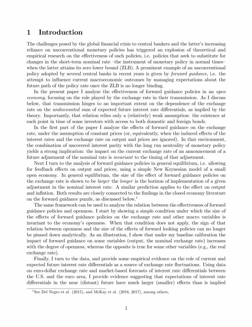
Assume that at time t the home central bank credibly announces an increase of the nominalinterest rate of size δ, starting T periods from now and of duration D (i.e., from period t+T tot+ T +D− 1), with no reaction expected from the foreign central bank. Furthermore, assumethat the path of domestic and foreign prices remains unchanged (this assumption is relaxedbelow). Both the transitory nature of the intervention, as well as the assumption of long runneutrality of monetary policy, imply that limT→∞ Et{qT} should not change in response to theprevious announcement. It follows from (6) that the real exchange rate will vary in responseto the announcement by an amount given by

qt = −Dδi.e. the exchange rate appreciation at the time of the announcement is proportional to theduration and the size of the announced interest rate increase, but is independent of its plannedtiming (T ). Thus, a D-period increase of the real interest rate 10 years from now is predictedto have the same effect on today’s real exchange rate as an increase of equal size and durationto be implemented immediately.Once the interest rate increase is effectively implemented in period t+T , the exchange rate

depreciates at a constant rate δ per period, i.e. ∆qt+T+k = δ for k = 1, 2, ..D and stabilizes atits initial level once the intervention concludes, i.e. qt+T+k = qt for k = D + 1, D + 2, ...Figure 1 illustrates that prediction by displaying the implied path of the interest rate and

the exchange rate when an interest rate rise of 1% (in annual terms) is announced at t = 0, tobe implemented at T = 4 and lasting for D = 4 periods.

2See, e.g., Engel and West (2004, 2006), Chinn (2008), Mark (2009), Clarida and Walmann (2008), amongmany others.

4

4 Forward Guidance and the Exchange Rate in GeneralEquilibrium

Consider the (log-linearized) equilibrium conditions of a standard small open economy modelwith Calvo staggered price-setting, law of one price (producer pricing), and complete markets.3

πH,t = βEt{πH,t+1}+ κyt − ωqt (8)

yt = (1− υ)ct + ϑqt (9)

ct = Et{ct+1} −1

σ(it − Et{πt+1}) (10)

ct =1

σqt (11)

where πH,t ≡ pH,t−pH,t−1 denotes domestic inflation, yt is (log) output and ct is (log) consump-tion. Equation (8) is a New Keynesian Phillips curve for the small open economy. Coeffi cients κand ω are defined as κ ≡ λ (σ + ϕ) and ω ≡ λ(ση−1)υ(2−υ)

1−υ where υ ∈ [0, 1] is an index of openness(equal the share of imported goods in domestic consumption in the steady state), σ > 0 is the(inverse) elasticity of intertemporal substitution, η > 0 is the elasticity of substitution betweendomestic and foreign goods, and λ ≡ (1−θ)(1−βθ)

θ> 0 is inversely related to the Calvo price

stickiness parameter θ. (9) is the goods market clearing condition, with ϑ ≡ ηυ(1 + 1

1−υ)> 0.

(10) is the consumption Euler equation, with πt ≡ pt− pt−1 denoting CPI inflation. (11) is theinternational risk sharing condition, derived under the assumption of complete markets. Theabove specification of the equilibrium conditions assumes constant prices and real interest ratesin the rest of the world, normalized to zero for notational ease (i.e. r∗t = p∗t = 0 all t). Alsofor simplicity I abstract from any non-policy shocks, with the analysis focusing instead on theeffects of exogenous monetary policy changes.Note that (10) and (11) imply the real version uncovered interest parity analyzed in the

previous section:4

qt = Et{qt+1} − (it − Et{πt+1}) (12)

Furthermore, under the maintained assumption of full pass through, CPI inflation anddomestic inflation are linked by

πt ≡ (1− υ)πH,t + υ∆et

= πH,t +υ

1− υ∆qt (13)

As emphasized in Galí and Monacelli (2005) the previous equilibrium conditions can becombined to obtain a system of two difference equations for domestic inflation πH,t and outputyt that is isomorphic to that of the closed economy, namely:

πH,t = βEt{πH,t+1}+ κvyt (14)

3Detailed derivations of the equilibrium conditions can be found in Galí and Monacelli (2005) and Galí (2015,chapter 8) With little loss of generality I assume an underlying technology that is linear in labor input.

4The assumption of complete markets at the international level is suffi cient (though not necessary) to derivethe uncovered interest parity equation. As discussed in section 2 above that equation can be derived as long asthere are some investors each period with access to both domestic and foreign one-period bonds.

5

yt = Et{yt+1} −1

συ(it − Et{πH,t+1}) (15)

where συ ≡ σ1+(ση−1)υ(2−υ) > 0 and κv ≡ λ (συ + ϕ) > 0 are now both functions of the open

economy parameters (υ, η).In addition, combining (9) and (11) we can derive the following simple relation between the

real exchange rate and output:qt = συ(1− υ)yt (16)

In order to close the model, a description of monetary policy is required. I assume thesimple rule

it = φππH,t (17)

where φπ > 1. It can be easily checked that in the absence of exogenous shocks the equilibriumin the above economy is (locally) unique and given by πH,t = yt = qt = it = 0 for all t.

Consider next a forward guidance experiment analogous to the one analyzed in the previoussection, but allowing for an endogenous response of inflation to the anticipated change inthe interest rate. More specifically, assume that at time 0, the home central bank crediblyannounces a nominal interest rate one-period increase of 0.25 (i.e. one percentage point inannualized terms) in period T . Furthermore, the central bank commits to keeping the nominalinterest rate at its initial level (normalized to zero in the impulse responses) until period T − 1,independently of the evolution of inflation. At time T + 1 it restores the interest rate rule (17)and, with it, the initial equilibrium. I use (14), (15) and (16) to determine the response ofoutput, domestic inflation and the real exchange rate to that forward guidance experiment.Given the response of πH,t and qt, (13) can be used to back out the response of CPI inflation,πt. The latter can then be used to derive the response of the (consumption) price level, whichcombined with the relation et = qt+pt allows one to derive the response of the nominal exchangerate.Figure 2 displays the response of interest rates, the exchange rate, output, and inflation, to

the above experiment under three alternative time horizons for implementation: T = {1, 2, 4}.The parameters of the model are calibrated as follows: β = 0.99, υ = 0.4, σ = ϕ = 1, η = 2, andθ = 0.75. Note that a version of the "forward guidance puzzle" for the open economy emerges:the longer is the horizon of implementation, the larger is the impact of the announcement onthe real and nominal exchange rates as well as on output and inflation. As emphasized byMcKay el at. (2016), the reason for the amplification has to do with the fact that inflationdepends on current and expected future output, combined with the property that the longer isthe implementation of a given interest rise the more persistent the output response. It followsthat the longer is the implementation horizon of a given change in the nominal rate the largerwill be the response of the real rate —and hence of output and the real exchange rate—betweenthe time of the announcement and that of policy implementation.Figure 3 illustrates more explicitly the forward guidance puzzle as applies to the nominal

and real exchange rates. It displays the percent response of those two variables on impactwhen a one-period increase in the nominal rate is announced, to be implemented at alternativehorizons represented by the horizontal axis. As the Figure makes clear the percent appreciationof the home currency, both in real and nominal terms, increases exponentially with the horizonof implementation. Note also that the appreciation of the nominal exchange rate is substantially

6

larger than that of the real exchange rate, with the gap between the two increasing with thehorizon of implementation. That gap, which corresponds to the percent decrease in the CPIin response to the forward guidance announcement, is also increasing in the horizon due tothe forward-lookingness of the New Keynesian Phillips curve. The fall in inflation, in turn,leads to a further rise in current and future real interest rates, thus generating an additionalappreciation of the real exchange rate.An alternative perspective on the previous experiment can be obtained by focusing on the

determination of the nominal exchange rate. Consider an announcement of an interest rateincrease of size δ and duration D, to be implemented T periods ahead. Iterating forwardequation (4) we can express the nominal exchange rate at the time of the policy announcementas:

et = δD + Et{et+T+D}= δD + Et{pt+T+D} (18)

The first term on the right hand side of (18) captures the dependence of the nominalexchange rate on anticipated changes in nominal interest rate differentials. As discussed insection 2 that effect is a function of the size (δ) and duration (D) of the anticipated policyintervention, but not of its timing. This captures the partial equilibrium dimension of theforward guidance exchange rate puzzle. The second term, Et{pt+T+D}, which reinforces theeffect of the first term, is the result of general equilibrium effects working through (i) theimpact on aggregate demand and output of the changes in consumption and the real exchangerate induced by the anticipation of higher future nominal interest rates (given prices), and (ii)their subsequent effects on inflation and the price level, which depend on the duration of theoutput effects (as implied by (14)) and, hence, on the timing of the policy implementation.The strength of some the general equilibrium effects pointed out above is, from an empirical

perspective, a controversial subject. This is true, in particular, with regard to the forward-lookingness of inflation, i.e. that variable’s sensitivity to expected future output developments.An empirical analysis of those general equilibrium channels in the determination of exchangerates is clearly beyond the scope of the present paper.5 Instead, in the remainder of the paper Iturn to an empirical exploration of the (partial equilibrium) link between the exchange rate andfuture interest rate differentials, with a focus on the role played by the horizon of anticipatedinterest rate changes.

5 Interest Rate Expectations and the Exchange Rate:Does the Horizon Matter?

In the present section I examine the evidence on the extent to which fluctuations in the euro-dollar real exchange rate can be accounted for by variations in expected interest rate differentialsat different horizons. I start by defining the following two variables measuring anticipated real

5See, e.g. Mavroeidis et al. (2014), Rudd and Whelan (2005) and Galí et al. (20015), as well as othercontributions to the special issue of the Journal of Monetary Economics (vol. 52, issue 6) on the empirics ofthe New Keynesian Phillips curve for a discussion of some the issues in that controversy.

7

interest rate differentials at short and long horizons:

qSt (M) ≡M−1∑k=0

Et{r∗t+k − rt+k}

qLt (M) ≡T−1∑k=M

Et{r∗t+k − rt+k}

for any 0 < M < T and given a "large" long-term horizon T . Note that qSt (M) is a measureof the expected interest rate differentials over the short run (i.e. over the next M periods),while qLt (M) captures the corresponding effect of expected interest rate differentials at a longerhorizon (i.e. beyond the next M periods, and up to T ). Below I report OLS estimates of theregression equation

qt = α0 + α1t+ α2t2 + γSq

St (M) + γLq

Lt (M) + εt (19)

using the empirical counterparts to qSt (M) and qLt (M) described below for the US and the euroarea. Note that coeffi cients γS and γL measure the reduced form (semi) elasticities of the realexchange rate with respect to the short term and long term component of expected real interestrate differentials.As a benchmark, consider the implications of the theoretical model introduced in section 2.

Equilibrium condition (5) combined with rational expectations implies:

qt = qSt (M) + qLt (M) + Et{qt+T} (20)

Again, let qt = ft + qt with ft a deterministic trend such that limT→∞ Et{qt+T} is bounded.Assuming that the stochastic component of the real exchange rate, qt, is a stationary processwith zero mean, so that, for large T , Et{qt+T} ' limT→∞ Et{qt+T} = 0, one can rewrite (20) as:

qt = qSt (M) + qLt (M) + ft+T (21)

Under the assumption (confirmed by the evidence below) that the long run trend in the(log) real exchange rate can be approximated by a quadratic function of time, equation (21) isconsistent with empirical equation (19) with γS = γL = 1, thus providing a useful theoreticalbenchmark. As noted above, the absence of discounting in (21) implies that, ceteris paribus,a change in qSt (M) (given qLt (M)) should have the same effect on the real exchange rate as acommensurate change in qLt (M) (given qSt (M)). Furthermore, that effect should be "one-for-one" in both cases.In order to estimate (19) I need to construct empirical counterparts to qSt (M) and qLt (M).

This requires some assumptions, which I take as reasonable approximations, given the purposeat hand. Thus, and given that the empirical analysis makes use of monthly data, the annualizednominal yield on a M -period bond is assumed to satisfy

it(M) =12

M

M−1∑k=0

Et{it+k}

where it(1) ≡ it, i.e. the interest rate on a one-month nominally riskless bond. Subtracting(annualized) expected inflation between t and t + M from both sides of the previous equationwe can write:

rt(M) =12

M

M−1∑k=0

Et{rt+k}

8

An analogous expression holds for foreign bonds. Thus, it follows that,

qSt (M) =M

12[r∗t (M)− rt(M)] (22)

I construct measures of r∗t (M) and rt(M) using monthly data on German and US governmentbond zero coupon yields with 2, 5, 10 and 30 year maturity (thus corresponding to M ∈{24, 60, 120, 360}), combined with monthly measures of expected inflation over the same fourhorizons derived from inflation swaps. Constraints on data availability for the latter variableforce me to start the sample period in 2004:8. Given the time series for real interest rates atdifferent horizons thus obtained, I use (22) to construct a time series for qSt (M) for different Mvalues.In order to obtain an empirical counterpart to qLt (M) I set T = 360 (corresponding to a 30

year horizon) and then use the relation:

qLt (M) ≡ qSt (T )− qSt (M)

I construct a monthly time series for the (log) real exchange rate qt, using data on the (log)euro-dollar nominal exchange rate, and the (log) CPI indexes for the US and the euro area.

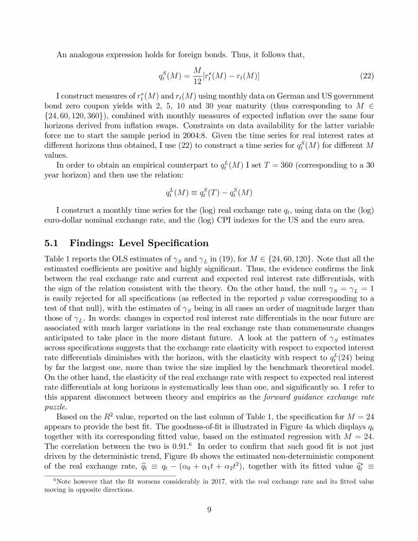
5.1 Findings: Level Specification

Table 1 reports the OLS estimates of γS and γL in (19), forM ∈ {24, 60, 120}. Note that all theestimated coeffi cients are positive and highly significant. Thus, the evidence confirms the linkbetween the real exchange rate and current and expected real interest rate differentials, withthe sign of the relation consistent with the theory. On the other hand, the null γS = γL = 1is easily rejected for all specifications (as reflected in the reported p value corresponding to atest of that null), with the estimates of γS being in all cases an order of magnitude larger thanthose of γL. In words: changes in expected real interest rate differentials in the near future areassociated with much larger variations in the real exchange rate than commensurate changesanticipated to take place in the more distant future. A look at the pattern of γS estimatesacross specifications suggests that the exchange rate elasticity with respect to expected interestrate differentials diminishes with the horizon, with the elasticity with respect to qLt (24) beingby far the largest one, more than twice the size implied by the benchmark theoretical model.On the other hand, the elasticity of the real exchange rate with respect to expected real interestrate differentials at long horizons is systematically less than one, and significantly so. I refer tothis apparent disconnect between theory and empirics as the forward guidance exchange ratepuzzle.Based on the R2 value, reported on the last column of Table 1, the specification forM = 24

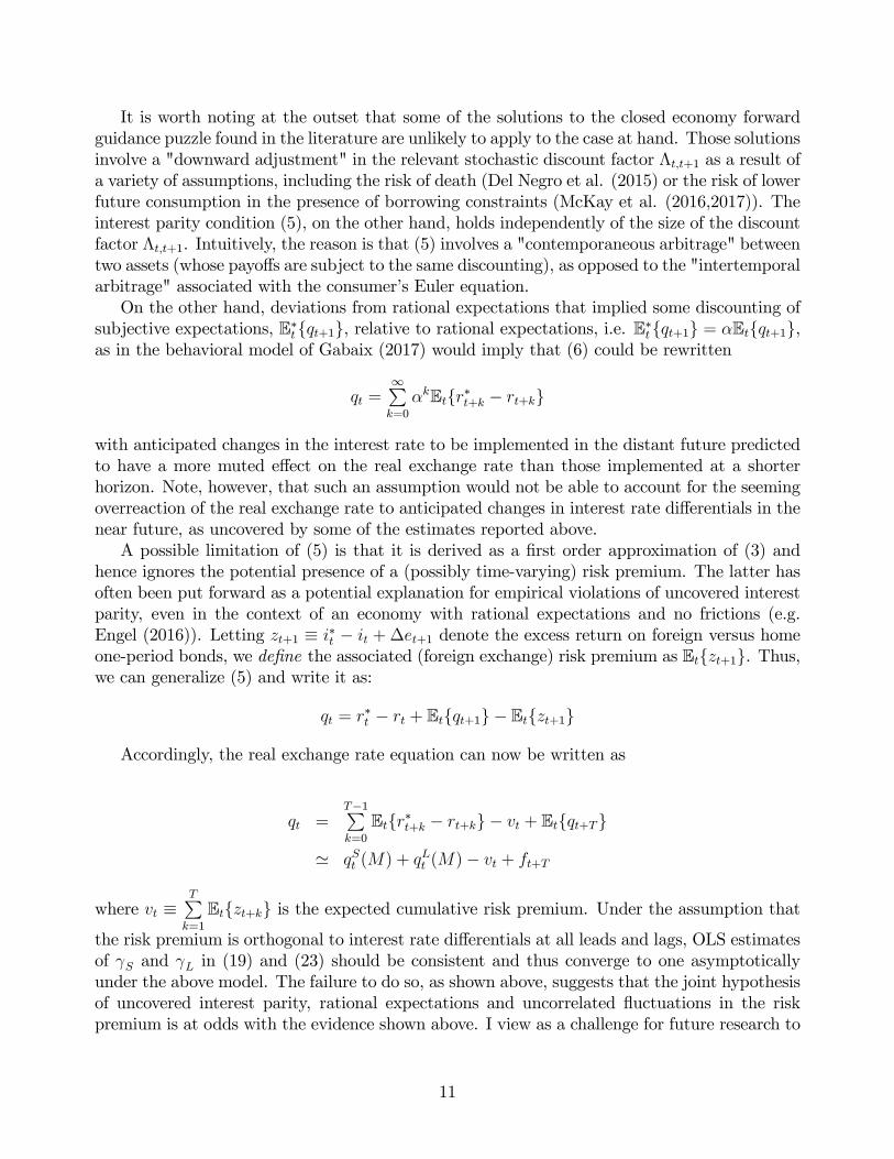
appears to provide the best fit. The goodness-of-fit is illustrated in Figure 4a which displays qttogether with its corresponding fitted value, based on the estimated regression with M = 24.The correlation between the two is 0.91.6 In order to confirm that such good fit is not justdriven by the deterministic trend, Figure 4b shows the estimated non-deterministic componentof the real exchange rate, qt ≡ qt − (α0 + α1t + α2t

2), together with its fitted value q∗t ≡6Note however that the fit worsens considerably in 2017, with the real exchange rate and its fitted value

moving in opposite directions.

9

γSqSt (M) + γLq

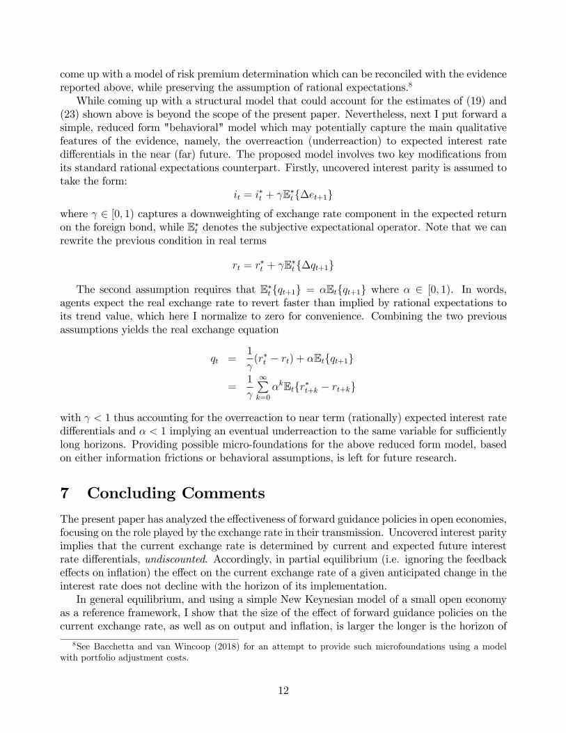
Lt (M). Their correlation is, again, very high: 0.85. Finally, Figure 5 further

decomposes q∗t into q∗,St ≡ γSq

St (M) and q∗,Lt ≡ γLq

Lt (M), and points to the dominant role of

expected interest rate differentials less than two years ahead in accounting for fluctuations in qt,with the correlation between qt and q

∗,St being equal to 0.58. By contrast, expected interest rate

differentials beyond the two-year horizon seem to play a small role in accounting for short termfluctuations in the real exchange rate, possibly with the exception of the 2015-2017 period. Onthe other hand, q∗,Lt and qt appear to display a much higher correlation at lower frequencies,with the gradual decline in expected real interest rate differentials beyond two years seeminglydriving the gradual real appreciation of the US dollar until 2016. The correlation between qtand q∗,Lt over the full sample period is equal to 0.64.

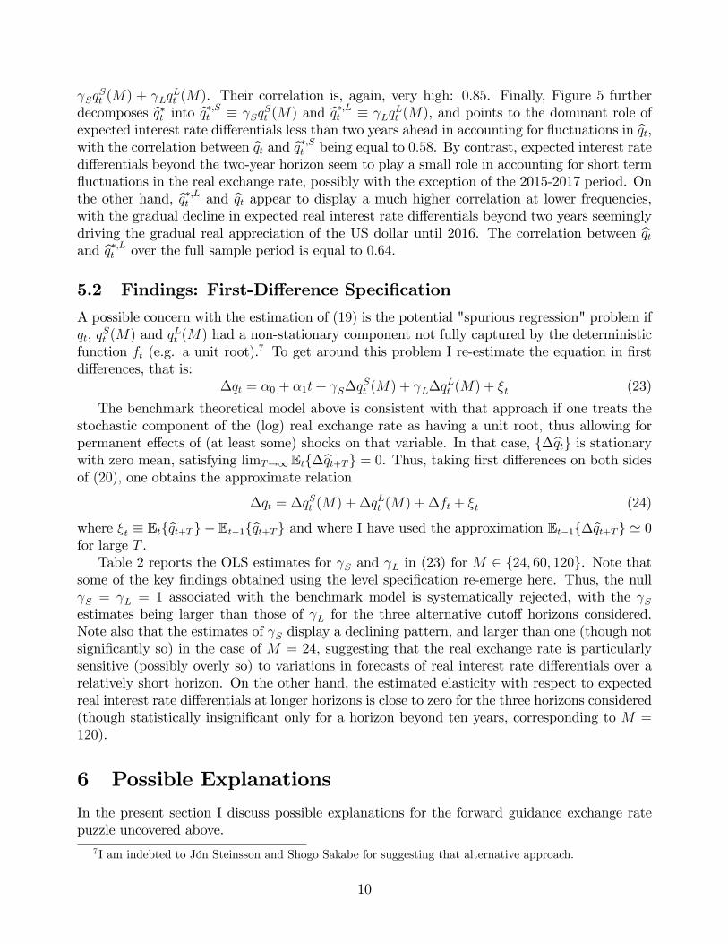
5.2 Findings: First-Difference Specification

A possible concern with the estimation of (19) is the potential "spurious regression" problem ifqt, qSt (M) and qLt (M) had a non-stationary component not fully captured by the deterministicfunction ft (e.g. a unit root).7 To get around this problem I re-estimate the equation in firstdifferences, that is:

∆qt = α0 + α1t+ γS∆qSt (M) + γL∆qLt (M) + ξt (23)

The benchmark theoretical model above is consistent with that approach if one treats thestochastic component of the (log) real exchange rate as having a unit root, thus allowing forpermanent effects of (at least some) shocks on that variable. In that case, {∆qt} is stationarywith zero mean, satisfying limT→∞ Et{∆qt+T} = 0. Thus, taking first differences on both sidesof (20), one obtains the approximate relation

∆qt = ∆qSt (M) + ∆qLt (M) + ∆ft + ξt (24)

where ξt ≡ Et{qt+T} − Et−1{qt+T} and where I have used the approximation Et−1{∆qt+T} ' 0for large T .Table 2 reports the OLS estimates for γS and γL in (23) for M ∈ {24, 60, 120}. Note that

some of the key findings obtained using the level specification re-emerge here. Thus, the nullγS = γL = 1 associated with the benchmark model is systematically rejected, with the γSestimates being larger than those of γL for the three alternative cutoff horizons considered.Note also that the estimates of γS display a declining pattern, and larger than one (though notsignificantly so) in the case of M = 24, suggesting that the real exchange rate is particularlysensitive (possibly overly so) to variations in forecasts of real interest rate differentials over arelatively short horizon. On the other hand, the estimated elasticity with respect to expectedreal interest rate differentials at longer horizons is close to zero for the three horizons considered(though statistically insignificant only for a horizon beyond ten years, corresponding to M =120).

6 Possible Explanations

In the present section I discuss possible explanations for the forward guidance exchange ratepuzzle uncovered above.

7I am indebted to Jón Steinsson and Shogo Sakabe for suggesting that alternative approach.

10

It is worth noting at the outset that some of the solutions to the closed economy forwardguidance puzzle found in the literature are unlikely to apply to the case at hand. Those solutionsinvolve a "downward adjustment" in the relevant stochastic discount factor Λt,t+1 as a result ofa variety of assumptions, including the risk of death (Del Negro et al. (2015) or the risk of lowerfuture consumption in the presence of borrowing constraints (McKay et al. (2016,2017)). Theinterest parity condition (5), on the other hand, holds independently of the size of the discountfactor Λt,t+1. Intuitively, the reason is that (5) involves a "contemporaneous arbitrage" betweentwo assets (whose payoffs are subject to the same discounting), as opposed to the "intertemporalarbitrage" associated with the consumer’s Euler equation.On the other hand, deviations from rational expectations that implied some discounting of

subjective expectations, E∗t{qt+1}, relative to rational expectations, i.e. E∗t{qt+1} = αEt{qt+1},as in the behavioral model of Gabaix (2017) would imply that (6) could be rewritten

qt =∞∑k=0

αkEt{r∗t+k − rt+k}

with anticipated changes in the interest rate to be implemented in the distant future predictedto have a more muted effect on the real exchange rate than those implemented at a shorterhorizon. Note, however, that such an assumption would not be able to account for the seemingoverreaction of the real exchange rate to anticipated changes in interest rate differentials in thenear future, as uncovered by some of the estimates reported above.A possible limitation of (5) is that it is derived as a first order approximation of (3) and

hence ignores the potential presence of a (possibly time-varying) risk premium. The latter hasoften been put forward as a potential explanation for empirical violations of uncovered interestparity, even in the context of an economy with rational expectations and no frictions (e.g.Engel (2016)). Letting zt+1 ≡ i∗t − it + ∆et+1 denote the excess return on foreign versus homeone-period bonds, we define the associated (foreign exchange) risk premium as Et{zt+1}. Thus,we can generalize (5) and write it as:

qt = r∗t − rt + Et{qt+1} − Et{zt+1}

Accordingly, the real exchange rate equation can now be written as

qt =T−1∑k=0

Et{r∗t+k − rt+k} − vt + Et{qt+T}

' qSt (M) + qLt (M)− vt + ft+T

where vt ≡T∑k=1

Et{zt+k} is the expected cumulative risk premium. Under the assumption thatthe risk premium is orthogonal to interest rate differentials at all leads and lags, OLS estimatesof γS and γL in (19) and (23) should be consistent and thus converge to one asymptoticallyunder the above model. The failure to do so, as shown above, suggests that the joint hypothesisof uncovered interest parity, rational expectations and uncorrelated fluctuations in the riskpremium is at odds with the evidence shown above. I view as a challenge for future research to

11

come up with a model of risk premium determination which can be reconciled with the evidencereported above, while preserving the assumption of rational expectations.8

While coming up with a structural model that could account for the estimates of (19) and(23) shown above is beyond the scope of the present paper. Nevertheless, next I put forward asimple, reduced form "behavioral" model which may potentially capture the main qualitativefeatures of the evidence, namely, the overreaction (underreaction) to expected interest ratedifferentials in the near (far) future. The proposed model involves two key modifications fromits standard rational expectations counterpart. Firstly, uncovered interest parity is assumed totake the form:

it = i∗t + γE∗t{∆et+1}where γ ∈ [0, 1) captures a downweighting of exchange rate component in the expected returnon the foreign bond, while E∗t denotes the subjective expectational operator. Note that we canrewrite the previous condition in real terms

rt = r∗t + γE∗t{∆qt+1}

The second assumption requires that E∗t{qt+1} = αEt{qt+1} where α ∈ [0, 1). In words,agents expect the real exchange rate to revert faster than implied by rational expectations toits trend value, which here I normalize to zero for convenience. Combining the two previousassumptions yields the real exchange equation

qt =1

γ(r∗t − rt) + αEt{qt+1}

=1

γ

∞∑k=0

αkEt{r∗t+k − rt+k}

with γ < 1 thus accounting for the overreaction to near term (rationally) expected interest ratedifferentials and α < 1 implying an eventual underreaction to the same variable for suffi cientlylong horizons. Providing possible micro-foundations for the above reduced form model, basedon either information frictions or behavioral assumptions, is left for future research.

7 Concluding Comments

The present paper has analyzed the effectiveness of forward guidance policies in open economies,focusing on the role played by the exchange rate in their transmission. Uncovered interest parityimplies that the current exchange rate is determined by current and expected future interestrate differentials, undiscounted. Accordingly, in partial equilibrium (i.e. ignoring the feedbackeffects on inflation) the effect on the current exchange rate of a given anticipated change in theinterest rate does not decline with the horizon of its implementation.In general equilibrium, and using a simple New Keynesian model of a small open economy

as a reference framework, I show that the size of the effect of forward guidance policies on thecurrent exchange rate, as well as on output and inflation, is larger the longer is the horizon of

8See Bacchetta and van Wincoop (2018) for an attempt to provide such microfoundations using a modelwith portfolio adjustment costs.

12

implementation of the announced policies. Under my baseline calibration, the size of the effectsof forward guidance policies on some variables (output, nominal exchange rate) is increasing inthe degree of openness, but it is decreasing for some other variables (e.g. real exchange rate).Using data on the euro-dollar real exchange rate and market-based forecasts of real interest

rate differentials between the U.S. and the euro area, I provide evidence that conflicts with theprediction of undiscounted effects of anticipated real interest rate differentials. In particular,expectations of interest rate differentials in the near (distant) future appear to have much larger(smaller) effects than is implied by the theory, an observation which I refer to as the forwardguidance exchange rate puzzle. Further research to provide a theoretical explanation to thatpuzzle seems warranted.

13

REFERENCES

Angeletos, George-Marios and Chen Lian (2017): "Forward Guidance without CommonKnowledge," mimeo.Bacchetta, Philippe and Eric van Wincoop (2018): "Exchange Rates, Interest Rates and

Gradual Portfolio Adjustment," work in progress.Carlstrom, charles T., Timothy S. fuerst, Matthias Paustian (2015): "Inflation and Output

in New Keynesian Models with a Transient Interest Rate Peg," Journal of Monetary Economics76, 230-243Cook, David and Michael Devereux (2013): "Exchange Rate Flexibility under the Zero

Lower Bound: The Need for Forward Guidance," mimeo.Eggertsson, Gauti, and Michael Woodford (2003): “The Zero Bound on Interest Rates and

Optimal Monetary Policy,”Brookings Papers on Economic Activity, vol. 1, 139-211.Gabaix, Xavier (2017): "A Behavioral New Keynesian Model," mimeo.Engel, Charles (2016): "Exchange Rates, Interest Rates and the Risk Premium," American

Economic Review 106(2), 436-474.Galí, Jordi, Mark Gertler, David López-Salido (2005): “Robustness of the Estimates of

the Hybrid New Keynesian Phillips Curve,”Journal of Monetary Economics, vol. 52, issue 6,1107-1118.Galí, Jordi, and TommasoMonacelli (2005): “Monetary Policy and Exchange Rate Volatility

in a Small Open Economy,”Review of Economic Studies, vol. 72, issue 3, 2005, 707-734Galí, Jordi (2015): Monetary Policy, Inflation and the Business Cycle: An Introduction to

the New Keynesian Framework, Second edition, Princeton University Press (Princeton, NJ),chapter 6.Del Negro, Marco, Marc P. Giannoni, and Christina Patterson (2015) "The Forward Guid-

ance Puzzle," mimeo.Jung, Taehun, Yuki Teranishi, and Tsutomo Watanabe, (2005): "Optimal Monetary Policy

at the Zero Interest Rate Bound," Journal of Money, Credit and Banking 37 (5), 813-835.Mavroeides, Sophocles, Mikkel Plagborg-Moller, and James H. Stock (2014): "Empirical

Evidence on Inflation Expectations in the New Keynesian Phillips Curve," Journal of EconomicLiterature 52(1), 124-188.McKay, Alisdair, Emi Nakamura and Jon Steinsson (2016): "The Power of Forward Guid-

ance Revisited," American Economic Review, 106(10), 3133-3158,McKay, Alisdair, Emi Nakamura and Jon Steinsson (2015): "The Discounted Euler Equa-

tion: A Note," Economica, forthcoming.Rudd, Jeremy and Karl Whelan (2005): "New Tests of the New Keynesian Phillips Curve,"

Journal of Monetary Economics, vol. 52, issue 6, 1167-1181.

14

Table 1. Empirical Exchange Rate EquationLevel speci�cationb S b L p R2

M=24 2:74(0:24)

�� 0:26(0:03)

�� 0:00 0:83

M=60 1:70��(0:16)

0:18��(0:03)

0:00 0:81

M=120 0:98(0:13)

�� 0:12��(0:04)

0:00 0:77

Note: The table reports the OLS estimates of S and L in theregression equation

qt = �0 + �1t+ �2t2 + Sq

St (M) + Lq

Lt (M) + "t

using monthly data spanning the sample period 2004:8-2017:12. Thep statistic corresponds to the null hypothesis S = L = 1. Twoasterisks indicate signi�cance at 5 percent level.

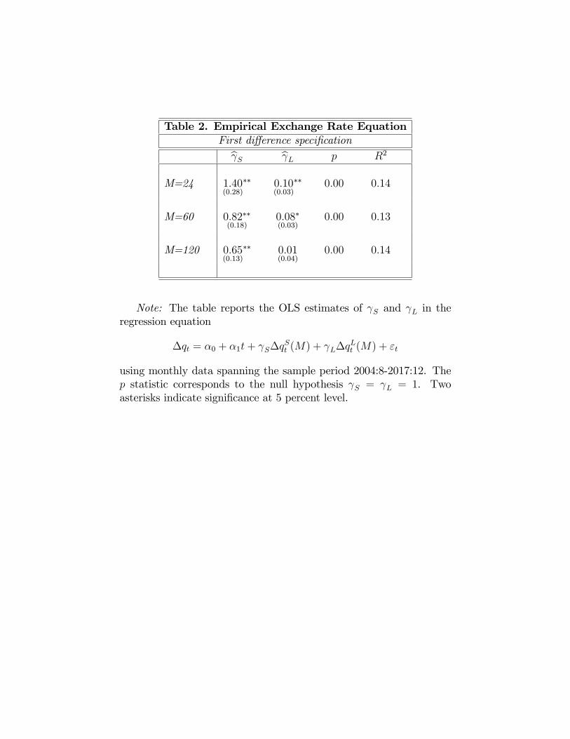
Table 2. Empirical Exchange Rate EquationFirst di¤erence speci�cationb S b L p R2

M=24 1:40(0:28)

�� 0:10(0:03)

�� 0:00 0:14

M=60 0:82��(0:18)

0:08�(0:03)

0:00 0:13

M=120 0:65(0:13)

�� 0:01(0:04)

0:00 0:14

Note: The table reports the OLS estimates of S and L in theregression equation

�qt = �0 + �1t+ S�qSt (M) + L�q

Lt (M) + "t

using monthly data spanning the sample period 2004:8-2017:12. Thep statistic corresponds to the null hypothesis S = L = 1. Twoasterisks indicate signi�cance at 5 percent level.

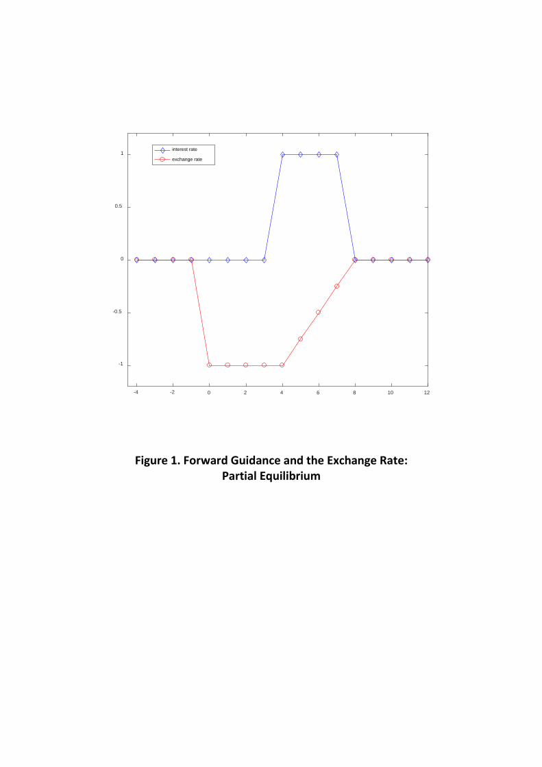
Figure 1. Forward Guidance and the Exchange Rate:

Partial Equilibrium

-4 -2 0 2 4 6 8 10 12

-1

-0.5

0

0.5

1interest rate

exchange rate

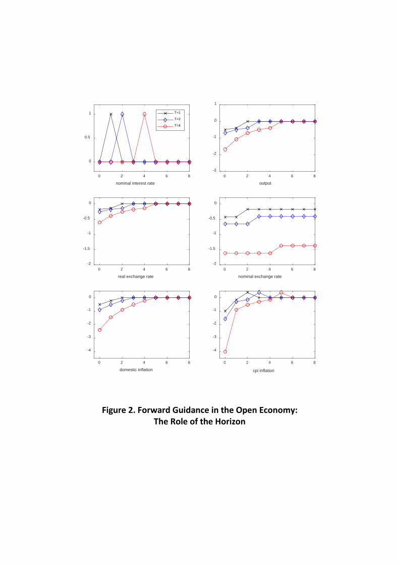
Figure 2. Forward Guidance in the Open Economy: The Role of the Horizon

0 2 4 6 8

real exchange rate

-2

-1.5

-1

-0.5

0

0 2 4 6 8

domestic inflation

-4

-3

-2

-1

0

0 2 4 6 8

output

-3

-2

-1

0

1

0 2 4 6 8

nominal exchange rate

-2

-1.5

-1

-0.5

0

0 2 4 6 8

cpi inflation

-4

-3

-2

-1

0

0 2 4 6 8

nominal interest rate

0

0.5

1 T=1

T=2

T=4

Figure 3. The Forward Guidance Exchange Rate Puzzle

0 1 2 3 4 5 6 7 8 9 10

horizon

-30

-25

-20

-15

-10

-5

0ex

chan

ge ra

te re

spon

se (%

)

nominal

real

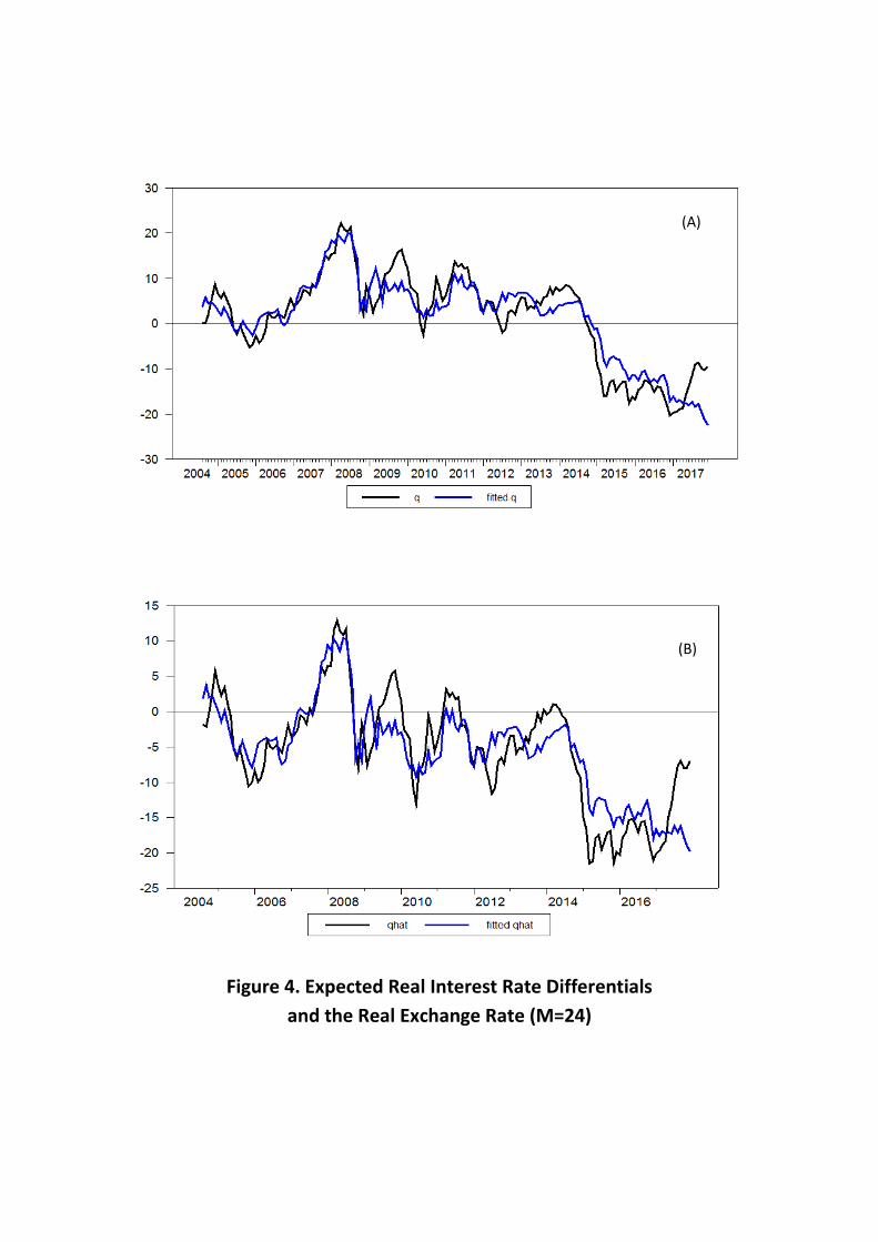
Figure 4. Expected Real Interest Rate Differentials and the Real Exchange Rate (M=24)

(B)

(A)

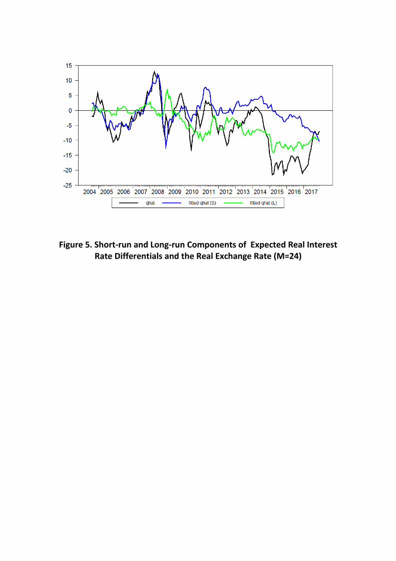
Figure 5. Short-run and Long-run Components of Expected Real Interest Rate Differentials and the Real Exchange Rate (M=24)