forthcoming in: The Review of Economic Studies

Beyond Icebergs: Toward A Theory of Biased Globalization

By Kiminori Matsuyama1

The Final Version

Abstract

In contrast to domestic trade, international trade inherently requires moreintensive use of skilled labor with expertise in areas such as internationalbusiness, language skills, and maritime insurance, and the transoceanictransportation is more capital intensive than the local transportation. In thepresence of such bias in factor demands, globalization caused by an improvementin the export technologies can lead to a world-wide increase in the relative pricesof the factors used intensively in international trade. Furthermore, a world-wideincrease in the factors used intensively in international trade can lead toglobalization. To capture these effects, we develop a flexible approach to modelcostly international trade, which includes the standard iceberg approach as aspecial case. More specifically, we extend the Ricardian model of trade with acontinuum of goods (Dornbusch, Fischer and Samuelson, 1977) by introducingmultiple factors of production and by making technologies of supplying goodsdepend on whether the destination is home or abroad. If the technologies ofsupplying the same good to the two destinations differ only in total factorproductivity, the model becomes isomorphic to the DFS Ricardian model with theiceberg cost. By allowing the two technologies to differ in the factor intensities,our approach enables us to examine the links between factor endowments, factorprices and globalization that cannot be captured by the iceberg approach.

JEL Classifications: F11 (Neoclassical Models of Trade), F15 (EconomicIntegration)Keywords: Biased Globalization, Costly Trade, Export Technologies, IcebergCost, Factor Prices, Skill Premia

1Department of Economics, Northwestern University, 2001 Sheridan Road, Evanston, IL 60208-2600, USA.http://www.faculty.econ.northwestern.edu/faculty/matsuyama/. I would like to thank Daron Acemoglu, GadiBarlevy, Gene Grossman, Bob Lucas, Jimmy Roberts, Mathias Thoenig, the referees, and the editor for theircomments and suggestions, and Toulouse Network on Information Technology for financial support.

1

1. Introduction.

This paper proposes a flexible approach to model costly international trade.2 The key

idea is to make the technologies of supplying goods depend on the destinations.3 By using the

word, “supply,” we mean to include all the activities associated with delivering the goods to the

customers in a particular market. It includes not only the production and the physical shipment

of the goods, but also the marketing and customer services, which involve communication with

the dealers, customers, and government agencies, as well as the services related to export

financing and maritime insurance. Under the assumption that it is more costly to supply goods to

the export market than to the domestic market, this approach naturally leads to the home market

bias, deviations from the law of one price, and generates endogenously nontraded goods (i.e., the

goods that are potentially “tradeable” but not traded in equilibrium.)

Our approach includes the standard approach of modeling costly trade, the iceberg

approach, as a special case. According to this approach, commonly attributed to Samuelson

(1954), the technologies of producing the goods are the same, regardless of whether the

destination of the goods is home or abroad. The cost of trade takes the form of “shrinkage” in

transit so that only a fraction of the good shipped abroad actually arrives. Our approach would

become isomorphic to the iceberg approach if we add the restriction that the technologies of

supplying the goods to different markets differ only in total factor productivity. Our approach is

more flexible than the iceberg approach because it allows for the possibility that supplying the

goods abroad may use the factors in a different proportion from supplying the goods at home.

This flexibility enables us to explore the links between factor endowments, factor prices, and

globalization that cannot be captured by the iceberg approach.

For example, imagine that the cost of supplying the goods abroad declines relative to the

cost of supplying domestically. Such a change in the relative cost can happen for many different

reasons, e.g., advances in information technology (telegraphs, telephones, facsimiles, internet,

communication satellites, etc), a tariff reduction, a harmonization of the regulations across

countries, a wider acceptance of English as the global business language, an emergence of the

global consumer culture that reduces the need for the goods to be tailor-made for each country, 2 For the empirical significance of trade costs, see a survey by Anderson and van Wincoop (2004).

2

etc. The resulting globalization means a reallocation of the factors from the activities associated

with supplying the goods to the domestic market to those associated with supplying the goods to

the export market. If we were to model this process by a reduction in the iceberg cost,

globalization could change relative factor demands only through the standard Stolper-Samuelson

effect. That is to say, relative factor demands of a country could change only when the country’s

exported goods and its imported goods have different factor intensities. This also means that

globalization would tend to move the factor prices in different directions in different countries.

If the wage rate of white-collar workers relative to blue-collar workers goes up in one country

because of the factor content of its net exports, then the relative wage of white-collar workers

must go down in its trading partners. Our approach has a different implication. If exporting

goods inherently require more intensive use of some factors (say, white-collar workers,

particularly those with language skills, international business experiences and/or specialists in

export finance and maritime insurance) than supplying the same goods domestically,

globalization may lead to an increase in the relative price of these factors in all of the countries.

To give another example, the standard factor proportion theory of trade, such as the

Heckscher-Ohlin model, relies on the cross-country difference in factor proportions as a basis of

international trade, and hence it does not have a clear prediction as to how the volume of trade

responds when the factor proportions change in the same direction across countries. Our model

has a different implication, because the factor endowments affect international trade in a more

direct manner. If servicing the foreign customers requires more skilled labor, if the transoceanic

transportation is more capital intensive than the local transportation, etc., a world-wide increase

in the relative supply of these factors will lead to globalization.

Obviously, one could apply our approach to any existing model of international trade that

uses the iceberg approach. In this paper, we have chosen the Ricardian model with a continuum

of goods, developed by Dornbusch, Fischer, and Samuelson (1977), hereafter DFS. For a variety

of reasons, their model offers a useful background against which to demonstrate our approach.

First, the Ricardian structure of the DFS model enables us to illustrate the difference between our

approach and the iceberg approach without the additional complication of the well-understood

3 Deardorff (1980) also allowed for the technologies to depend on the destination. However, he did not pursue anyof the issues investigated in this paper.

3

Hechscher-Ohlin-Stolper-Samuelson effects. Second, to the best of our knowledge, DFS is the

first study that derived the set of nontraded goods endogenously by making use of the iceberg

approach. Furthermore, DFS has inspired many recent studies on competitive models of

international trade with the iceberg approach.4

Section 2 develops our model, which extends the DFS model in two respects. First, it has

multiple factors of production. Second, the technologies of supplying each good depend on

whether the destination is the domestic or export market, and it is assumed that it is more costly

to supply the good abroad than at home. Section 3 considers the special case, where the

technologies of supplying the goods to the two markets differ only in total factor productivity.

With this additional restriction, an improvement in the export technologies5 leads to

globalization, but has no effect on the relative factor prices, and the factor proportions play no

role in determining the extent of globalization. Indeed, it is demonstrated that this special case is

isomorphic to the DFS model with the iceberg cost. Section 4 considers the general case, where

the technologies may differ also in factor intensity. It shows how an improvement in the export

technologies and a change in the factor proportions lead to globalization as well as a change in

the relative factor prices. Section 5 considers an application to the debate on the role of

globalization in the recent rise in the skill premia. Under the assumption that exporting goods

requires more intensive use of skilled labor than supplying the same goods to the domestic

market, it is shown that a world-wide increase in the relative supply of skilled labor leads to

globalization, in sharp contrast to Heckscher-Ohlin. It is also shown that globalization, when it is

caused by (Hicks-neutral) technical change in the export sectors, by (Hicks-neutral) skilled-labor

augmenting technical change, or by a reduction in trade barriers, leads to a rise in the skill premia

in all the countries, in sharp contrast to Stolper-Samuelson. Section 6 concludes.

4See, e.g., Obstfeld and Rogoff (1996, Chapter 4), Eaton and Kortum (2002), and Alvarez and Lucas (2004).Another literature that makes extensive use of the iceberg approach is monopolistic competition models of trade.Unlike these models, the DFS model has the advantage of highlighting the difference between the two approacheswithout the complications of the market structure, monopoly power, and expanding product variety.5By “an improvement in the export technologies,” we mean general technical changes that improve the efficiency ofsupplying the goods to the foreign markets (relative to the domestic market), which are not specific to a particulargood or industry. It should not be confused with “an export-biased technical change,” the well-known concept thatcan be found in most standard textbooks of international trade, first proposed by Hicks (1953). The latter is anindustry-specific technical change that improves the efficiency of production in an exporting industry. This type oftechnical change does not change the cost of supplying the same good to the foreign markets relative to the domesticmarket. It changes the relative cost of producing the exportable goods to the importable goods.

4

2. The Framework

Consider the following variation of the DFS (1977) model. The world economy consists

of two countries, Home and Foreign, and there are a continuum of competitive industries,

identified by the good it produces, z � [0,1]. The Home consumers have the identical Cobb-

Douglas preferences with b(z) being the expenditure share of good z, with �1

0

b(z)dz = 1. Thus,

the Home demand for good z is given by D(z) = b(z)E/p(z), where p(z) is the Home price of good

z and E is the Home aggregate expenditure. Likewise, the Foreign demand for good z is D*(z) =

b*(z)E*/p*(z), where b*(z) is the Foreign expenditure share of good z, with �1

0

b*(z)dz = 1,

p*(z) is the Foreign price of good z, and E* is the Foreign aggregate expenditure.

This paper departs crucially from DFS in two respects. First, there are J factors of

production, with V = (V1, V2, …, VJ)T and V* = (V1*, V2*, … , VJ*)T being the column vectors

of the Home and Foreign factor endowments, where Vj and Vj* are the Home and Foreign

endowments of the j-th factor (j = 1, 2, …, J). The factors are nontradeable and the factor prices

are given by the row vectors, w = (w1, w2, … , wJ) and w* = (w1*, w2*, …, wJ*). We may think

of these factors not only as capital, land, and labor, but also as different types of labor, with

different skill levels, expertise, and specialties. Second, the technologies may depend on the

destination of goods. More specifically, we may think of each industry consisting of two sectors:

a domestic sector and an export sector. The domestic sector of industry z at Home can supply

one unit of good z to the Home market at a cost of a(z)Φ(w), while its export sector can supply

one unit of good z to the Foreign market at a cost of a(z)Ψ(w;τ). It should be noted that the

word, “supply,” here includes all of the activities needed to deliver the good to the consumers in

a particular market. It includes not only the production cost, but also the marketing costs,

including all sorts of communication costs and shipping costs, including the insurance and other

financial costs.6 Both Φ and Ψ are assumed to be linear homogeneous, increasing, and concave

6 Recall that we identify “industries” and “sectors” by the goods they produce and by the market they serve. Hence,all the factors that go into the same good must be considered as part of the same industry, even though they may beemployed by many different firms scattered across many different industries. Likewise, all the factors that go intothe same goods heading for the same destination must be considered as a part of the same sectors. For example, the

5

in w. Thus, they satisfy the standard properties of the unit cost functions associated with CRS

technologies.7 Likewise, the unit cost of the domestic sector of the Foreign industry z is

a*(z)Φ*(w*), while the unit cost of the export sector of the Foreign industry z is a*(z)Ψ*(w*;

τ*). Note the presence of the shift parameters, τ and τ*, in the cost functions of the export

sectors. We will use them to examine the effect of the technical change in the export sectors.8

Furthermore, we will make the following assumptions.

(A1) A(z) ≡ a*(z)/a(z) is continuous and decreasing in z.

(A2) Φ(w) < Ψ(w;τ); Φ*(w*) < Ψ*(w*;τ*).

The first assumption, (A1), is borrowed directly from DFS. It means that the goods are indexed

according to the patterns of comparative advantage; Home (Foreign) has comparative advantage

in lower (higher) indexed goods. (A2) implies that supplying (i.e., producing, marketing,

shipping, insuring etc.) goods to the export market is more costly than supplying (i.e., producing,

marketing, shipping, insuring etc.) goods to the domestic market. This model may be viewed as

a hybrid of the Ricardian model of trade and the factor proportion models of trade. Across the

goods (and industries), the technologies differ only in total factor productivity, but not in factor payment made by a manufacturer or a distributor and received by the insurer for its coverage of the domestic(international) shipping has to be included in the cost of the domestic (export) sector, just like the payment for anyraw materials that go into the goods supplied to the domestic (export) market has to be included in the cost of thedomestic (export) sector. In other words, to the extent that the factors employed in the maritime insurance industryare involved, either directly or indirectly, in exporting a particular good, they should be considered as a part of thesame export sector, even if its manufacturer, its distributor, and its insurer may be in different categories in thestandard industry classification.7 Some readers might think that certain activities required for exporting impose the fixed cost for an exporting firm.The presence of the fixed cost for a firm does not invalidate our assumption that each sector has CRS technologies.As Alfred Marshall and many others pointed out, the correct unit of analysis in a competitive model is the industry orthe sector, not the firm. The firm level fixed cost can be the variable cost at an industry level, because the size of theindustry changes as the number of firms in the industry adjusts. (Any introductory economics textbook shouldexplain how the U-shaped average cost curve of a firm is consistent with the constant average cost curve of anindustry.)8 By allowing the unit cost function of the Home (Foreign) export sector to depend solely on the factor prices atHome (Foreign), this specification implicitly assumes that exporting goods does not require any factors local to theexport market. Of course, it would be more realistic to assume that US exports to Italy generate demand for factorsin Italy and that Italian exports to the US generate demand for factors in the US (particularly in the service sectors).To allow for this possibility, Matsuyama (2005, section 6.1) extends the present model to let the unit cost function ofthe Home (Foreign) export sector to depend also on w* (w) and shows that such an extension does not affect thebasic mechanism. (One could also allow the unit cost function of the domestic sector to depend on the foreign factor

6

intensity. Within each industry, on the other hand, the domestic and export sectors may differ not

only in total factor productivity, but also in factor intensity. It should be noted, however, that,

unlike the standard factor proportion models of trade, the factor intensity differences are based on

the destination of the goods, not on the goods themselves. We deliberately rule out the factor

intensity differences across goods, in order to isolate our result from the well-known Hechscher-

Ohlin-Stolper-Samuelson mechanism.9

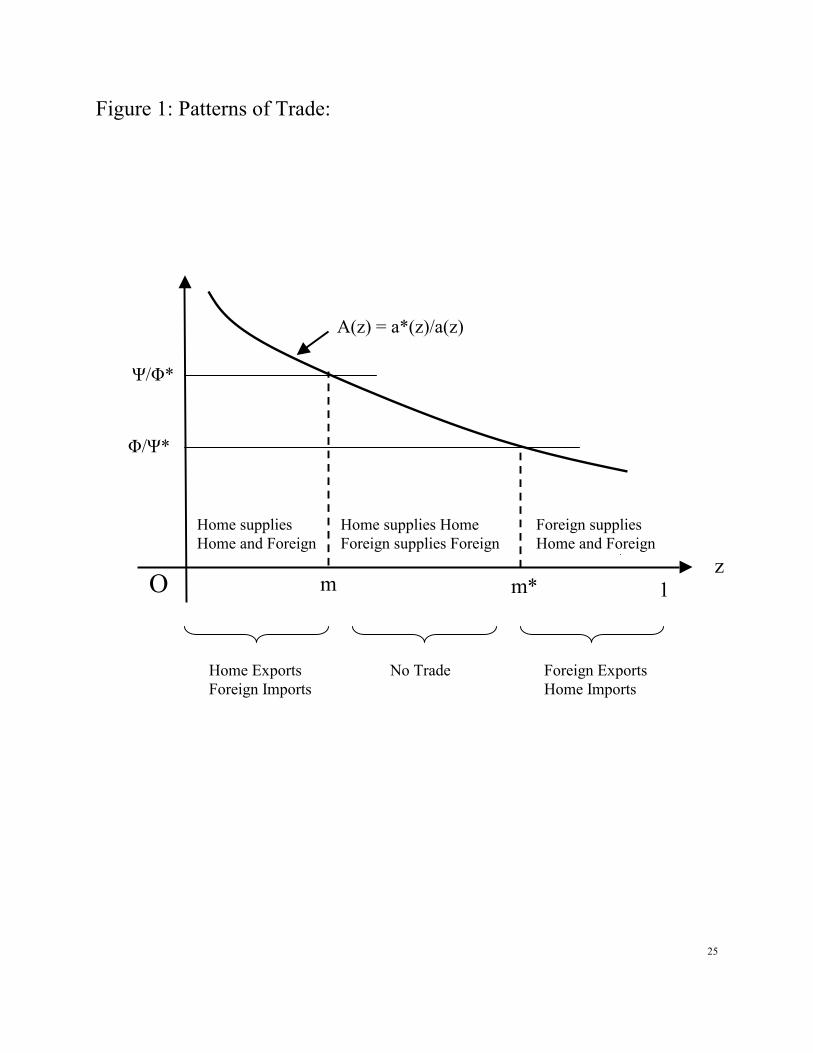
The consumers everywhere purchase the goods from the lowest cost suppliers. Hence,

the price of good z is equal to p(z) = min{a(z)Φ(w), a*(z)Ψ*(w*;τ*)} and p*(z) =

min{a(z)Ψ(w;τ), a*(z)Φ*(w*)}. Assumptions (A1) and (A2) thus imply that, for any factor

prices, w and w*, there are two marginal industries, m < m*,

(1) A(m) = Ψ(w;τ)/Φ*(w*),

(2) A(m*) = Φ(w)/Ψ*(w*;τ*),

such that only the Home industries supply to the Home and Foreign markets in z � [0,m), only

the Foreign industries supply to the Home and Foreign markets in z � (m*,1], and only the Home

industries supply to the Home market and only the Foreign industries supply to the Foreign

market in z � (m,m*). In other words, Home exports and Foreign imports in z � [0, m) and

Home imports and Foreign exports in z � (m*, 1]. There is no trade in z � (m, m*). These

goods are endogenously nontraded goods (i.e., potentially tradeable goods that are not traded in

equilibrium). The patterns of production and trade are illustrated in Figure 1.

From the standard result of the duality theory of production (see, e.g., Dixit and Norman

1980), each unit of good z produced and purchased in Home generates demand for Home factor j

equal to a(z)Φj(w) = p(z)Φj(w)/Φ(w), where subscript j signifies the partial derivative with

respect to wj. Similarly, each unit of good z produced in Home and purchased in Foreign

generates demand for Home factor j equal to a(z)Ψj(w;τ) = p*(z)Ψj(w;τ)/Ψ(w;τ). Thus, the

equilibrium condition for the market for Home factor j is given by

prices to allow for the possibility of international outsourcing. Again, such an extension merely complicates thenotation without affecting the basic mechanism.)9 It should be pointed out, however, that our approach can be applied to a Heckscher-Ohlin model, as well. SeeMatsuyama (2005, section 6.2).

7

Vj = [Φj(w)/Φ(w)] �*

0

m

[p(z)D(z)]dz + [Ψj(w;τ)/Ψ(w;τ)] �m

0

[p*(z)D*(z)]dz, (j = 1, 2,…J),

where the first (second) term of the RHS is the derived demand for Home factor j from supplying

goods to the domestic (export) market. By using p(z)D(z) =b(z)E and p*(z)D*(z) = b*(z)E*, this

condition can be rewritten to

Vj = [Φj(w)/Φ(w)]B(m*)E + [Ψj(w;τ)/Ψ(w;τ)]B*(m)E*, (j = 1, 2,…J)

where B(z) ≡ �z

0

[b(s)]ds and B*(z) ≡ �z

0

[b*(s)]ds are the Home and Foreign expenditure shares

of the goods in [0, z]. They are strictly increasing and satisfy B(0) = B*(0) = 0 and B(1) = B*(1)

= 1. This condition can be further simplified as

(3) wjVj = αj(w)B(m*)wV + βj(w;τ)B*(m)w*V* (j = 1, 2,…J)

by defining αj(w) ≡ wjΦj(w)/Φ(w) and βj(w;τ) ≡ wjΨj(w;τ)/Ψ(w;τ), and making use of the budget

constraints in the two countries, E = wV and E* = w*V*. Eq. (3) is easily interpreted. Since

B(m*) is the fraction of the Home aggregate income spent on the Home industries and αj(w) is

the share of factor j in the domestic sector of the Home industries, the first term of the RHS of

eq. (3) is the income earned by Home factor j derived from the domestic market. The second

term is the income earned by Home factor j derived from the export market, because B*(m) is the

fraction of the Foreign aggregate income spent on the Home industries, and βj(w;τ) is the share of

factor j in the export sector of the Home industries.

Similarly, the equilibrium condition for the market for Foreign factor j is given by

(4) wj*Vj* = αj*(w*)[1−B*(m)]w*V* + βj*(w*;τ*)[1−B(m*)]wV, (j = 1, 2,…J),

where αj*(w*) ≡ wj*Φj*(w*)/Φ*(w*) is the share of factor j in the domestic sector of the Foreign

industries; βj*(w*;τ*) ≡ wj*Ψj*(w*;τ*)/Ψ*(w*;τ*) is the share of factor j in the export sector of

8

the Foreign industries; 1−B(m*) is the fraction of the Home aggregate income spent on the

Foreign industries; and 1−B*(m) is the fraction of the Foreign aggregate income spent on the

Foreign industries.

Recall that the linear homogeneity of Φ(w) and Ψ(w) implies��

J

j 1αj(w) =

��

J

j 1βj(w;τ) = 1. Hence, adding up (3) for all j yields

(5) [1−B(m*)]wV = B*(m)w*V*.

This may be viewed as the balanced trade condition, as the LHS is the total value of the Foreign

exports and the RHS is the total value of the Home exports. Likewise, adding up (4) for all j also

yields eq. (5). This means that each of eq. (3) and eq. (4) offers J −1 independent equilibrium

conditions in addition to eq. (5). Thus, eqs. (1)-(5) altogether contain 2J+1 independent

equilibrium conditions. They jointly determine 2J+1 unknowns: the two marginal industries, m

and m*, and 2J −1 relative factor prices (i.e., 2J absolute factor prices, w and w*, up to a scale.)

We can use eqs. (1)-(5) to examine the effects of factor endowments, by shifting V and V*, as

well as the effects of globalization caused by technological change in the export sectors, by

shifting the two parameters, τ and τ*.

3. Unbiased Globalization: Restoring DFS (1977).

Let us first consider the following special case of (A2).

(A3) Ψ(w;τ) = τΦ(w) with τ > 1; Ψ*(w*;τ*) = τ*Φ*(w*) with τ* > 1.

Thus, the cost function of the export sector can be obtained by a homogeneous shift of the cost

function of the domestic sector. This assumption thus implies that both sectors have the same

factor intensity: βj(w;τ) = αj(w) and βj*(w*;τ*)= αj*(w*). The two sectors differ only in total

factor productivity. Furthermore, the technical change in the export sectors, a shift in τ and τ*,

satisfies Hicks-neutrality.

With (A3) and using eq. (5), eqs. (1)-(4) become

9

(6) A(m) = τΦ(w)/Φ*(w*),

(7) A(m*) = Φ(w)/τ*Φ*(w*),

(8) wjVj = αj(w)wV, (j = 1, 2,…J)

(9) wj*Vj* = αj*(w*)w*V*, (j = 1, 2,…J)

To simplify the above equations further, let us define F(x) ≡ minq {qx | Φ(q) ≥ 1}. It is

linear homogeneous, increasing and concave in x, and satisfies Φ(w) ≡ minx {wx | F(x) ≥ 1}.

Thus, it can be interpreted as the primal functions underlying Φ(w), where the technologies of the

domestic and export sectors of the Home industry z may be described by F(VD(z))/a(z) and

F(VE(z))/τa(z), where VD(z) and VE(z) are the vector of factors used in the domestic and export

sectors of industry z. Since all the J factors are used in the same proportion in all the activities in

equilibrium, they must be used in the same proportion with the factor endowment in equilibrium.

Hence, since Fj is homogeneous of degree zero, wj = p(z)Fj(V)/a(z) = p*(z)Fj(V)/τa(z) =

Φ(w)Fj(V) for all j. Therefore, from the linear homogeneity of F,

(10) wV = Φ(w)F(V) = WL,

where W and L are defined by W ≡ Φ(w) and L ≡ F(V). In other words, we can aggregate all the

factors into the single quantity index, “labor”, L = F(V), with the single price index, “the wage

rate,” W = Φ(w).10 Likewise, by defining F*(x) ≡ minq {qx | Φ*(q) ≥ 1},

(11) w*V* = Φ*(w*)F*(V*) = W*L*,

where the quantity index, L* = F*(V*), is the Foreign “labor” endowment and the price index,

W* = Φ*(w*), is the Foreign “wage rate.” Using (10)-(11), eqs. (5)-(7) become

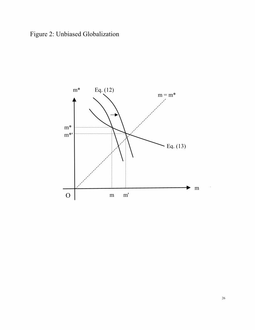
(12) A(m)/τ = W/W* = B*(m)L*/[1−B(m*)]L,

10Recall that W = Φ(w) and L = F(V) are scalars, while w is a J-dimensional row vector and V is a J-dimensionalcolumn vector.

10

(13) A(m*)τ* = W/W* = B*(m)L*/[1−B(m*)]L,

while (8) and (9) become

(14) Vj = Φj(w)L, (j = 1, 2,…J),

(15) Vj* = Φj*(w*)L*, (j = 1, 2,…J).

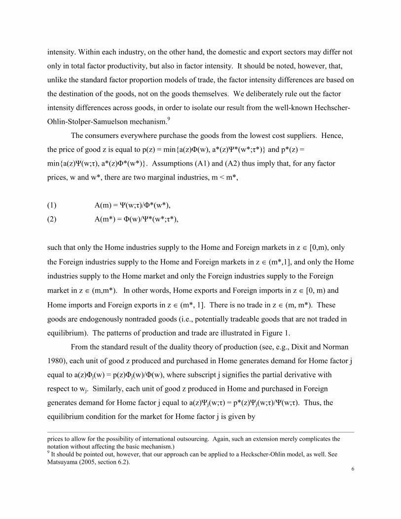
Note that eqs. (12)-(13) jointly determine m and m* as a function of τ and τ*, as shown in

Figure 2. A decline in τ shifts the steeper curve, representing (12), to the right, and as a result,

leads to a higher m, a lower m*, and a higher W/W*. Note that an improvement in the Home

export technologies not only expands the Home export sectors but also the Foreign export

sectors. Intuitively, as the improved export technologies enable the Home export sectors to

replace the Foreign domestic sectors in (m, m'), the Home wage rate goes up relative to the

Foreign wage rate, which leads to a replacement of the Home domestic sectors by the Foreign

export sectors in (m*',m*). This causes a reallocation of the Home labor from the domestic

sectors in (m*', m*) to the export sectors in (m, m'). At the same time, the Foreign labor is

reallocated from the domestic sectors in (m, m') to the export sectors in (m*', m*). Likewise, a

decline in τ* leads to a lower m*, a higher m, and a lower W/W*. Thus, an improvement in the

export technologies, regardless of whether it takes place at Home or at Foreign, leads to a growth

of trade and a reallocation of labor from the domestic to export sectors in both countries.

Under (A3), however, this reallocation of labor from the domestic to the export sectors

does not have any effect on the relative factor prices within each country. Note that, eqs. (14)-

(15) are independent of τ and τ*, as well as of m, m*, and W/W*. The relative factor prices

within each country are determined solely by eqs. (14)-(15). Recall that technical change in the

export sectors is Hicks-neutral, hence their relative factor demands are unaffected. Furthermore,

the export sectors use all the factors in the same proportion with the domestic sectors. Hence, the

relative factor demands cannot change through the composition effect, either. When

11

globalization does not change the relative factor demands, it has no effect on the relative factor

prices.11

Note also that eqs. (12)-(13) are entirely independent of V and V*. Hence, the factor

proportions have no effect on the patterns of trade. This is because the change in the relative

factor prices would not affect the relative cost of the two sectors.12

It is worth pointing out that the above model, under (A3), is essentially the same with the

DFS model. For example, if we set τ = τ* = 1, then m = m* and eqs. (12)-(13) collapse into

A(m) = W/W* = B*(m)L*/[1−B(m)]L. This is isomorphic to the equilibrium condition of the

basic model of DFS (1977, Section I), except that they assumed B(z) = B*(z). This should come

as no surprise. The two critical departures of the present model from DFS (i.e., the multiplicity

of the factors and the distinction between the domestic and export sectors) are inconsequential in

this case, because (A3) means that all the activities have the same factor intensity, which allow

us to aggregate all the factors into the single composite, “labor,” as in the basic DFS model, and

because, with τ = τ* = 1, both the domestic and export sectors produce the identical goods with

the identical technologies, again as in the basic DFS model. DFS (1977, Section IIIB) also

extended their model to allow for transport costs. Following the iceberg model of Samuelson

(1954), they assumed that a fraction g of good z shipped to the export market actually arrives.

Therefore, in order to supply one unit of good z to the Foreign country, Home must produce and

ship 1/g units of good z, which makes the price of the Home good z in the Foreign market equal

to a(z)W/g. Eqs. (12)-(13) are identical to the equilibrium conditions for the DFS model with the

iceberg transport cost if we set τ = τ* = 1/g > 1. This suggests a broad interpretation of the

iceberg cost. Instead of thinking that each industry produces with the same technology both for

the domestic and export markets, but only a fraction of the goods shipped arrives to the export

market, one can think that the domestic and export sectors produce different goods, each tailor- 11This is because the source of comparative advantage is Ricardian in the present model. If the source ofcomparative advantage were Heckscher-Ohlin (i.e. if the factor intensity differs across the goods and the twocountries differ in the factor proportion), technical changes in the export sectors could change the factor pricesthrough the well-known Stolper-Samuelson effect, even when the domestic and export sectors use the factors in thesame proportion in each industry. See Matsuyama (2005, section 6.2).12This is because the source of comparative advantage is Ricardian in the present model. If the source ofcomparative advantage were Heckscher-Ohlin (i.e. the factor intensity differs across the goods and the two countriesdiffer in the factor proportion), factor endowments could affect the patterns of trade through the well-knownHeckscher-Ohlin effect, even when the domestic and export sectors use the factors in the same proportion in eachindustry. See Matsuyama (2005, section 6.2).

12

made for each market, and that the total factor productivity of the export sector is a fraction of

that of the domestic sector. As long as the two sectors use all of the factors in the same

proportion, these two specifications give identical results. In short, we can view a decline in the

iceberg cost as a special form of technical changes that benefits the export sectors.

According to this broad interpretation, however, a reduction in τ and τ* can occur not

only through an improvement in transport technologies, but also through any changes that help to

lower the cost of servicing the export markets. Such changes may include an improvement in

communication and information technologies (telegraphs, telephones, facsimiles, internet,

communication satellite, etc), a harmonization of the regulations across countries, a wider

acceptance of English as the common business language, and an emergence of the global

consumer culture that reduces the need for the goods to be tailor-made for each country.

Perhaps more importantly, this broad interpretation also suggests a natural way of going

beyond the iceberg specification. Once we start thinking about the possibility that the destination

of the good affects the technologies of supplying the good, we may start thinking about the

possibility that it affects not only the total factor productivity but also the factor intensity. A

priori, such a possibility would be difficult to deny. Exporting naturally requires and generates

more demand for skilled labor with expertise in areas such as international business, language

skills, and maritime insurance. The transoceanic transportation is more capital intensive than the

local transportation. As will be seen below, this opens up the possibility that factor proportion

changes in the same direction both at Home and Foreign lead to globalization, as well as the

possibility that a change in the export technologies, and the resulting growth of trade and

reallocation of the factors from the domestic to export sectors, lead to a change in the relative

factor prices in the same direction both at Home and Foreign.

Before proceeding, it is worth pointing out that one could reinterpret eqs. (12)-(15) as the

equilibrium conditions for the case where the domestic and export sectors share the same

technology, but the Foreign government imposes import tariffs on the Home goods at the

uniform rate of τ − 1, and the Home government imposes import tariffs on the Foreign goods at

the uniform rate equal to τ* − 1, under the assumption that the tariff revenues are entirely wasted

13

so that they do not affect the aggregate expenditure of the two countries.13 Then the above result

suggests that a reduction in the import tariffs leads to globalization (an increase in m and a

decline in m*), but it does not affect the relative factor prices under (A3).

4. Biased Globalization

We are now going to show how the factor proportions affect globalization and how

technical changes in the export technologies can affect the relative factor prices, if we drop the

restrictive assumption, (A3). Recall the equilibrium conditions are given by eqs. (1)-(5). Since

the key mechanism does not rely on the asymmetry between Home and Foreign (and introducing

asymmetry would merely obscure the key mechanism), let us focus on the case where the two

countries are the mirror images of each other. That is,

(M) A(z)A(1−z) = 1.

b(z) = b*(z), b(z) = b(1−z) (so that B(z) = B*(z) and B(z) + B(1−z) = 1 for z � [0,1/2]),

Φ = Φ*, Ψ = Ψ* (so that αj = αj*, βj = βj*), and τ = τ*, and V = V*.

Note that the symmetry does not mean that the two countries are identical. Rather, they are the

mirror images of each other. More specifically, because A(z) is strictly decreasing in z,

A(z)A(1−z) = 1 implies that A(z) > 1 for z � [0,1/2), A(1/2) = 1 and A(z) < 1 for z � (1/2,1].

Without these cross-country differences in total factor productivity, trade would not take place.

Under the mirror image assumption, the equilibrium is symmetric, w = w*, m = 1−m* <

½, and the equilibrium conditions are now reduced to

(16) A(m) = Ψ(w;τ)/Φ(w),

(17) Vj = {αj(w) + [βj(w;τ)−αj(w)]B(m)}wV/wj (j = 1, 2,…J).

Eq. (16) shows that, given the factor prices, an improvement in the export technologies (a change

in τ that causes a downward shift of Ψ) leads to an increase in m (and a decline in m* = 1−m).

13 Imagine, for example, that Foreign (Home) government confiscate a fraction 1−1/τ (1−1/τ*) of the Home (Foreign)goods and use them for the public goods, which enter in the preferences of their residents in a separable form.

14

The RHS of Eq. (17) is the demand for factor j. It shows that a shift in τ could affect the factor

demand for two separate routes. The first is through international trade. A higher m increases

the demand for the factors used more intensively in the export sectors (those with βj > αj) and

reduces demand for those used more intensively in the domestic sectors (those with βj < αj).

Thus, globalization can affect the factor demand by changing the composition between the

domestic and export sectors. The second is by changing the relative factor demand within the

export sectors, if βj(w;τ) depends on τ. Note that there is an important special case, where a shift

in τ could affect the factor demands only through the first route. This is the case where the

technical change in the export sectors satisfies Hicks-neutrality:

(A4) Ψ(w;τ) = τΨ(w) with τ > 1 and Ψ(w) > Φ(w).

In this case, βj(w;τ) is independent of τ, which allow us to simply drop τ and denote it as βj(w).

Under (A4), the RHS of eq. (17) no longer depends on τ. Thus, a shift in τ affects the factor

demands only by changing the composition of the domestic and export sectors.14

To analyze eqs. (16)-(17) further, let us consider the two-factor case (J = 2). Then, eqs.

(16)-(17) become

(18) A(m) = ψ(ω;τ)/φ(ω)

(19) ��������

���������

���

�

���

��

)()]();([)(1)()]();([)(

111

111

2

1

mBmB

VV ,

where ω ≡ w1/w2 (= ω* ≡ w1*/w2*) is the relative factor price; φ(ω) ≡ Φ(ω,1) = Φ(w1,w2)/w2,

ψ(ω;τ) ≡ Ψ(ω,1; τ) = Ψ(w1,w2; τ)/w2; α1(ω) = 1− α2(ω) and β1(ω; τ) = 1−β2(ω;τ) are the shares of

factor 1 in the domestic and export sectors. (Recall that Φ and Ψ are linear homogeneous and

that the factor shares, αj and βj, are homogeneous of degree zero). Note that the RHS of eq. (19)

is the demand curve for factor 1 relative to factor 2.

14On the other hand, a shift in τ cannot affect the factor demand only through the second route. This is because wemust assume βj(w;τ) = αj(w) in order to shut down the first route and hence βj becomes independent of τ.

15

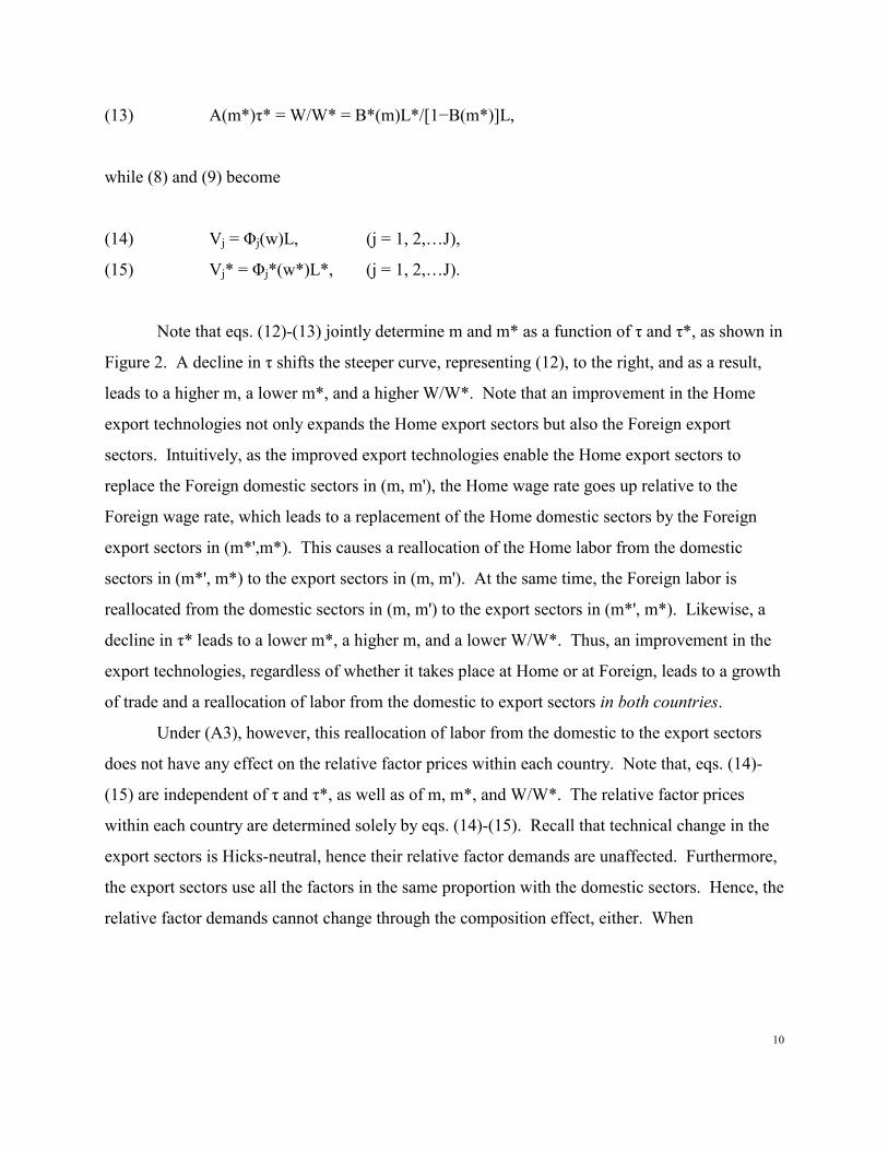
Figures 3 depict eqs. (18)-(19) over the (m, ω)-space, under the assumption that the

export sector is more factor 1 intensive than the domestic sector: α1(ω) < β1(ω;τ). This factor

intensity assumption implies that eq. (18) is downward-sloping.15 Intuitively, a lower ω makes

the cost of the export sectors decline more than the cost of the domestic sectors, and therefore

trade take places in a larger fraction of the industries (i.e., a higher m and a lower m* = 1−m).

Under the same factor intensity assumption, an expansion of the export sectors at the expense of

the domestic sector (a higher m and a lower m* = 1−m) leads to an increase in the relative

demand for factor 1. This in turn leads to a higher ω in a stable factor market equilibrium. Thus,

eq. (19) is upward-sloping, whenever the factor market is stable.16 Figures 3 are drawn under the

assumption that the factor market equilibrium is always stable, so that the curve depicting eq.

(19) is everywhere upward-sloping.17 The equilibrium is given by point E, at the intersection of

the two curves.

Figure 3a depicts the effects of an increase in V1/V2. It shifts the upward-sloping curve

downward, and the equilibrium moves from point E to point E'. The result is a decline in ω and

an increase in m. Note that, due to the symmetry assumption, this captures the effects of a world-

wide increase in the relative supply of the factor used more intensively in export activities. This

leads to a decline in the cost of supplying the foreign markets relative to the cost of supplying the

domestic markets, which leads to globalization, measured either in the share of the traded

industries, m+1−m* = 2m, or in the Trade/Income ratio, B*(m)+B(1−m*) = 2B(m). The effect is

thus different from the Heckscher-Ohlin mechanism, which relies on the difference in factor

proportions across the countries.

Figure 3b depicts the effects of a decline in τ, which shifts eq. (18), the downward-

sloping curve, to the right. Under (A4), i.e., when the improvement in the export technologies 15Algebraically, log-differentiating eq. (18) yields dω/dm = ωA'(m)/A(m)[β1(ω;τ)−α1(ω)] < 0.16To see this algebraically, let the RHS of eq. (19), the relative factor demand, be denoted by f(ω, m; τ). Then, β1(ω;τ) > α1(ω) implies fm > 0. The Walrasian stability of the factor market equilibrium requires that the relative demandcurve is decreasing in the relative price: i.e., fω < 0. Thus, dω/dm = − fm/fω > 0 along the stable factor marketequilibrium satisfying eq. (19).17This is the case, for example, if Φ and Ψ are Cobb-Douglas so that α1 and β1 are constant. Of course, withoutmaking some restrictions on the functional forms of Φ and Ψ, one cannot rule out the possibility that the relativefactor demand, f(ω, m; τ), may be increasing in ω over some ranges, and eq. (19) may permit multiple factor priceequilibriums. If so, the curve depicting eq. (19) over the (m, ω)-space could have an S-shape. In such a case, thedownward-sloping part corresponds to an unstable equilibrium, and hence only the upward-sloping parts are relevant

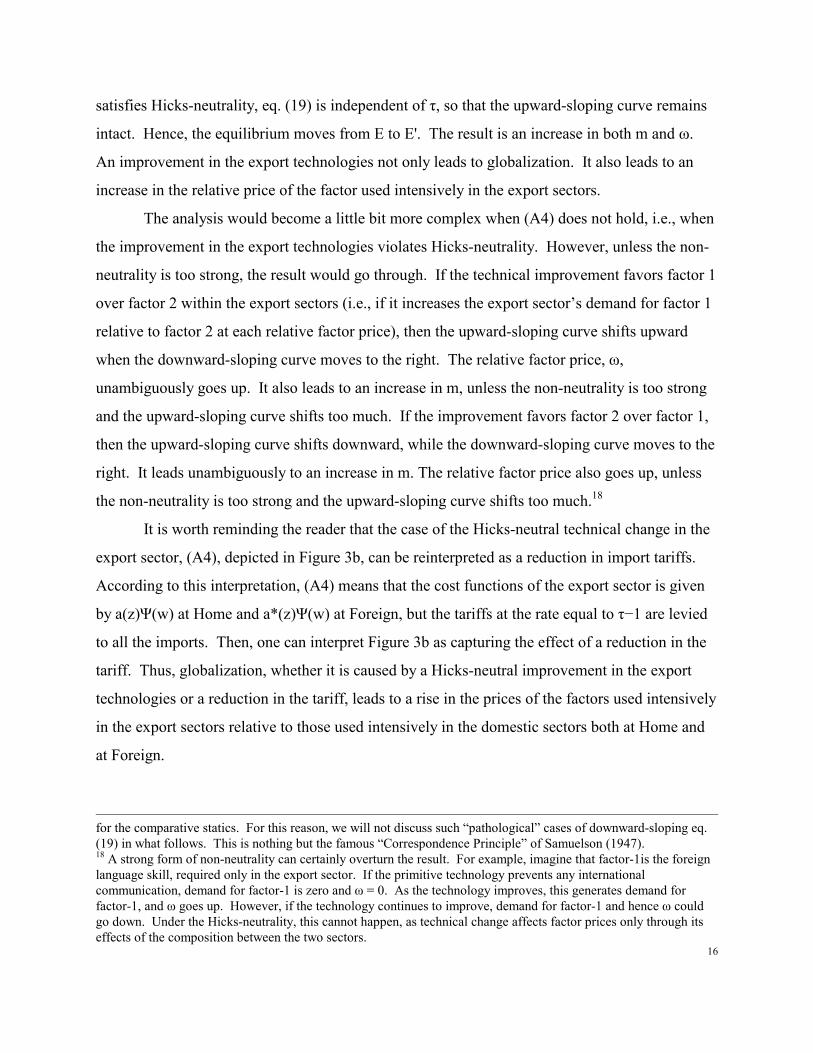
16

satisfies Hicks-neutrality, eq. (19) is independent of τ, so that the upward-sloping curve remains

intact. Hence, the equilibrium moves from E to E'. The result is an increase in both m and ω.

An improvement in the export technologies not only leads to globalization. It also leads to an

increase in the relative price of the factor used intensively in the export sectors.

The analysis would become a little bit more complex when (A4) does not hold, i.e., when

the improvement in the export technologies violates Hicks-neutrality. However, unless the non-

neutrality is too strong, the result would go through. If the technical improvement favors factor 1

over factor 2 within the export sectors (i.e., if it increases the export sector’s demand for factor 1

relative to factor 2 at each relative factor price), then the upward-sloping curve shifts upward

when the downward-sloping curve moves to the right. The relative factor price, ω,

unambiguously goes up. It also leads to an increase in m, unless the non-neutrality is too strong

and the upward-sloping curve shifts too much. If the improvement favors factor 2 over factor 1,

then the upward-sloping curve shifts downward, while the downward-sloping curve moves to the

right. It leads unambiguously to an increase in m. The relative factor price also goes up, unless

the non-neutrality is too strong and the upward-sloping curve shifts too much.18

It is worth reminding the reader that the case of the Hicks-neutral technical change in the

export sector, (A4), depicted in Figure 3b, can be reinterpreted as a reduction in import tariffs.

According to this interpretation, (A4) means that the cost functions of the export sector is given

by a(z)Ψ(w) at Home and a*(z)Ψ(w) at Foreign, but the tariffs at the rate equal to τ−1 are levied

to all the imports. Then, one can interpret Figure 3b as capturing the effect of a reduction in the

tariff. Thus, globalization, whether it is caused by a Hicks-neutral improvement in the export

technologies or a reduction in the tariff, leads to a rise in the prices of the factors used intensively

in the export sectors relative to those used intensively in the domestic sectors both at Home and

at Foreign.

for the comparative statics. For this reason, we will not discuss such “pathological” cases of downward-sloping eq.(19) in what follows. This is nothing but the famous “Correspondence Principle” of Samuelson (1947).18 A strong form of non-neutrality can certainly overturn the result. For example, imagine that factor-1is the foreignlanguage skill, required only in the export sector. If the primitive technology prevents any internationalcommunication, demand for factor-1 is zero and ω = 0. As the technology improves, this generates demand forfactor-1, and ω goes up. However, if the technology continues to improve, demand for factor-1 and hence ω couldgo down. Under the Hicks-neutrality, this cannot happen, as technical change affects factor prices only through itseffects of the composition between the two sectors.

17

Another thought-experiment that can be conducted by means of Figure 3b are the effects

of a change in A(z). Specifically, let us generalize A(z) to [A(z)]θ, where the power, θ > 0, is the

shift parameter. This keeps the mirror image assumption, and a higher θ raises [A(z)]θ for z �

[0, 1/2), and reduces [A(z)]θ for z � (1/2,1], thereby magnifying the cross-country difference in

total factor productivity in each industry. This change shifts the downward-sloping curve

upward, which leads to a higher m and a higher ω, as shown in Figure 3b. The intuition should

be clear. As the two countries become more dissimilar, there are more reasons to trade, which

shifts the demand in favor of the factors used more intensively in the export sectors.

5. An Application: Globalization, Technical Change, and Skill Premia

The model presented above can be useful for thinking about the debate on the role of

globalization in the recent rise in the skill premia. Imagine that there are two types of factors, J

=2, which are skilled and unskilled labor. Furthermore, suppose that the export sector is more

skilled labor intensive than the domestic sector. Under this interpretation of the model, Figure 3a

suggests that a world-wide increase in the relative supply of skilled labor leads to globalization.

Figure 3b suggests that the skill premia in all the countries rise as a result of globalization caused

by technical changes that take place in the export sectors (or by a reduction in the trade barriers).

However, we do not need to assume that the technical changes are specific to the export

sectors to obtain the above result. Skilled-labor augmenting technical changes can also have the

same effect, as long as we maintain the assumption that the export sector is more skilled-labor

intensive.

To see this, let us now modify the above model as follows. There are two factors, now

labeled as s for skilled labor and u for unskilled labor. The cost functions of the domestic and

export sectors of industry z are given by a(z)Φ(τws,wu) and a(z)Ψ(τws,wu) at Home and

a*(z)Φ*(τ*ws*, wu*) and a*(z)Ψ*(τ*ws, wu) at Foreign. Note that the shift parameters, τ and τ*,

enter in the cost functions of both the domestic and export sectors. Contrary to what was

assumed in the previous analysis, the technical changes are no longer specific to the export

sector. Now, a reduction in τ (and τ*) means a skilled-labor augmenting technical change, and

18

hence it reduces the costs of both the domestic and export sectors for fixed wage rates. We also

need to replace (A2) by

(A5) Φ(τws, wu) < Ψ(τws, wu) and Φ*(τ*ws*, wu*) < Ψ*(τ*ws*, wu*).

Then, by following the same steps as done in Section 2, we can conduct the analysis of this

modified model and derive its equilibrium conditions, analogous to eqs.(1)-(5).

Instead of repeating the whole analysis, let us focus on the case where the two countries

are the mirror-images of each other. Then, the equations analogous to eqs. (18)-(19) are given by

(20) A(m) = ψ(τω)/φ(τω),

(21) )()()]()([)(1

)()]()([)(/��

���������

������������

���

�

���

��

mBmB

VV

sss

sss

u

s ,

where ω ≡ ws/wu (= ω* ≡ ws*/wu*) is the price of skilled labor measured in unskilled labor. The

intuition behind eqs. (20)-(21) should be clear. Because a reduction in τ is now skilled-labor

augmenting, τ enters in these equations only through the “effective” price of skilled labor

measured in the units of unskilled labor, τω, and through the “effective” supply of skilled labor,

Vs/τ.

As before, we further focus on the special case, where the technical changes satisfy

Hicks-neutrality. A skilled labor augmenting technical change can be Hicks-neutral if and only

if the functional forms for Φ and Ψ are Cobb-Douglas.19 That is to say, we assume that

(A6) Φ(τws,wu) = (τws)α(wu)1−α, Ψ(τws,wu) = Г(τws)β(wu)1−β, 0 < α < β < 1.

where the parameter, Г, is sufficiently large to ensure that Φ(τws,wu) < Ψ(τws,wu) in equilibrium.

Then, eqs. (20)-(21) become

19We skip the proof because this is formally equivalent to the following well-known result in the neoclassical growthliterature, first shown by Uzawa (1961): technical changes are both Hicks-neutral (TFP-augmenting) and Harrod-neutral (labor-augmenting) if and only if the aggregate production function is Cobb-Douglas.

19

(22) A(m) = Г(τω)β−α,

(23) ����

�����

���

�

���

��

)()()1()()(mB

mBVV

u

s ,

respectively. These equations can be analyzed by means of Figure 3b. The assumption that the

export sector is more skilled-labor intensive, α < β, implies not only that eq. (22) is downward-

sloping and eq. (23) upward-sloping in the (m-ω) space. It also implies that a skilled-labor

augmenting technical change (a reduction in τ) shifts the downward-sloping curve to the right,

because it reduces the cost of the export sector more than the cost of the domestic sector. Hence,

it leads to globalization and an increase in skill premia. Needless to say, if we drop the

assumption of Hicks-neutrality, the analysis would be more complex, because eq. (21) generally

depends on τ. However, unless the non-neutrality is too strong, the effect would be qualitatively

similar.

In summary, we have shown the two scenarios in which globalization leads to a rise in the

skill premia in all the countries. In the first scenario, globalization is driven by (Hicks-neutral)

technical changes that take place in the export sectors (or by a reduction in the trade barriers). In

the second scenario, globalization is driven by the skilled-labor augmenting technical changes.

In both scenarios, the assumption that the export sector is more skilled-labor intensive than the

domestic sector plays a critical role.

This assumption is consistent with the empirical evidence that exporting manufacturing

firms employ more non-production workers than production workers, to the extent that non-

production workers may be viewed as a proxy for skilled labor, as is commonly done. Maurin,

Thesmar, and Thoenig (2002) offers more direct evidence, because their French dataset provides

detailed information on skill structure within both the production and non-production units of the

manufacturing firms. They have found that export firms employ more skilled labor than non-

exporters. Interestingly, they have found that the very act of exporting requires skilled labor

force. That is to say, more skilled labor is needed when they sell the products outside of France,

but the skill intensity does not vary much on whether they export to developed markets, such as

20

the US or to developing countries, such as China and India, which suggests that it is not the type

of products that determine the skill intensity.

It should be pointed out, however, that the existing empirical evidence based on

firm/plant level employment data within manufacturing, while largely consistent with our

assumption, is likely to underestimate the skill intensity of the export activities, because many

manufacturing firms rely on trading companies (such as the Japanese sogo shosha) and maritime

insurance companies for their export needs. The manufacturers outsource these services to such

companies presumably because they are more skilled in these activities. In order to account for

the factor content of the export goods properly, those working in the trading and insurance

sectors need to be included in the export sector to the extent that they are involved, directly or

indirectly, in the export activities.20

It is beyond the scope of this paper to survey the vast literature on the role of

globalization in the recent rise of the skill premia.21 Much of the literature draws a sharp

distinction between two possible causes; skill-biased technical change and international trade.

Most economists seem to discount the role of trade in favor of skill-biased technical changes for

a couple of reasons. First, according to the factor proportion theory of trade, an increase in trade

can explain the recent rise in the skill premium in the skilled-labor abundant United States, but

not the similar rise in the skill premia among the skilled-labor scarce trading partners. Second,

the factor proportion theory of trade also suggests that the rise in the skill premium in the U.S.

must be accompanied by a rise in the relative price of the skilled-labor intensive goods, which

has not been observed empirically. Our explanation is not subject to these criticisms because

what is skilled labor intensive in our model is trade itself, not the types of goods traded. 20 A relevant question is then: Do trading companies engaged more heavily in international trade employ moreskilled workers? Consider sogo shosha, Japanese general trading companies. These companies play a key role inthe Japanese foreign trade. They own worldwide networks of branches and stations through which they gatherinformation relevant to the trade. They trade a wide range of goods, ranging “from instant noodle to missiles” as awell-known expression puts it. The top nine general trading companies handle 47 percent of Japan’s exports, 65percent of imports (Ito, 1992, p.190). According to Yoshino and Lifton (1986, Ch.7), the most authoritative accountof sogo shosha available in English, “The firms recruit only from a limited number of universities, all of which arehighly selective institutions…. The sogo shosha has occupied an extremely privileged position…, for surveyresearch has consistently shown that, among graduating college students, the six sogo shosha have been consideredvirtually the most desirable private employers in Japan…. Whatever the reasons, the sogo shosha traditionally hashad little trouble in attracting what is considered to be the cream of the crop of Japanese college graduates to itsrecruitment process.” The same cannot be said about senmon shosha, trading companies specializing mostly indomestic trade.

21

Perhaps more importantly, our analysis questions the validity of the dichotomy between

skill- biased technical change and international trade. In this respect it is worth mentioning

Acemoglu and Zilibotti (2001, pp. 597-599), Acemoglu (2003), and Thoenig and Verdier (2003),

which developed models of endogenous technical changes to show how international trade

stimulates skill-biased technical changes. Their studies suggest that “globalization vs. skill-

biased technical changes” is a false dichotomy, because globalization induces skill-biased

technical change. The present study identifies the two scenarios that suggest that “globalization

vs. skill-biased technical changes” is a false dichotomy. According to the first scenario, it is a

false dichotomy, because globalization is inherently skill biased.22 According to the second

scenario, it is a false dichotomy, because globalization is induced by skilled-labor augmenting

technical changes.

Our approach also allows us to pose the following critical question, seldom asked in the

literature on trade and wages. What do we mean by “skilled labor”? After all, skilled labor is not

homogeneous; business majors and engineering majors are far from perfect substitutes. To

address this question, Matsuyama (2005, section 6.2) applies our approach of modeling costly

trade to the Heckscher-Ohlin model with a continuum of goods, a la Dornbusch, Fischer, and

Samuelson (1980). There are three factors: two types of skilled labor, those with business

degrees and those with engineering degrees, and unskilled workers. Home and Foreign share the

same technologies, but Foreign has a higher engineer/worker ratio than Home, and the industries

differ in the ratio of engineers to workers. Across all the industries, the export sectors use those

with business degrees more intensively than the domestic sectors. An improvement in the export

technology and the resulting globalization would increase the relative wage of those with

business degrees both at Home and at Foreign. In this sense, globalization contributes to the

global rise in the skill premia. However, the relative wage of engineers would go down at Home,

21For an overview of this literature, see Feenstra (2000).22Epifani and Gancia (2005a, b) also show that globalization is inherently skill biased, when the skill-intensivesectors are characterized by stronger increasing returns and different sectors produce highly substitutable goods. TheAcemoglu (and Acemoglu-Zilibotti) models rely on the asymmetry of the countries, and hence has the implicationthat North-South trade should be skill-biased. On the other hand, our model (and the Epifani and Gancia models)does not rely on the asymmetry of the countries, and hence suggests that all trade should be skill biased. This mightmake our argument more appealing to those who think that North-South trade is too small to have had much of aneffect. (We thank Daron Acemoglu for making this observation.)

22

where they are scarce, while it would go up at Foreign, where they are abundant, just as Stolper-

Samuelson predicts.

6. Concluding Remarks

If international trade generates more demand for certain factors than domestic trade,

globalization can directly affect the relative factor prices, and the factor proportions can directly

influence the extent of globalization. Exporting inherently requires the use of skilled labor with

expertise in areas such as international business, language skills, and maritime insurance. The

transoceanic transportation is more capital intensive than the local transportation. This opens up

the possibility that a world-wide increase in the factors used intensively in international trade

could lead to globalization, as well as the possibility that a change in the export technologies, and

the resulting globalization and reallocation of the factors from domestic trade to international

trade, could lead to a world-wide increase in the relative prices of the factors used intensively in

international trade. The standard approach to model costly international trade, the iceberg

approach, is too restrictive for capturing these effects.

In this paper, we explore a flexible approach to model costly international trade, which

includes the standard iceberg approach as a special case. To demonstrate our approach, we

extend the Ricardian model with a continuum of goods, due to Dornbusch, Fischer, Samuelson

(1977), by introducing multiple factors of production and by making technologies of supplying

goods depend on whether the destination is the domestic or export market. If the technologies of

supplying the good to different destinations differ only in total factor productivity, the model

becomes isomorphic to the DFS model with the iceberg cost. By allowing them to differ in the

factor intensities, our approach enables us to explore the links between factor endowments, factor

prices, and globalization that cannot be captured by the iceberg approach. For example, a world-

wide change in the factor proportion can lead to globalization, in sharp contrast to the Heckscher-

Ohlin effect, which relies on the cross-country difference in factor proportions. It is also shown

that an improvement in the export technologies changes the relative factor prices in the same

direction across countries, in sharp contrast to the usual Stolper-Samuelson effect, which

suggests that the relative factor prices move in different directions in different countries. We

also applied our analysis to the debate on globalization and the recent rise in the skill premia.

23

Although we have used the DFS model as a background to highlight the difference

between the two approaches, this modeling choice was made for simplicity. The assumption that

the source of comparative advantage is Ricardian – i.e., countries trade because of the exogenous

cross-country total factor productivity differences–, is not essential for the key mechanisms,

which rely on the differences in the factor demand composition between the export and domestic

activities. Indeed, Matsuyama (2005. section 6.2) demonstrates the same results within the

framework of the Heckscher-Ohlin model with a continuum of goods, developed by Dornbusch,

Fischer, and Samuelson (1980), where the source of comparative advantage is the exogenous

cross-country factor proportion differences.

More broadly, the iceberg specification has been used in many different classes of

models. Consider, for example, monopolistic competition models of trade, where, starting from

Krugman (1980), the iceberg specification is the most common way of modeling costly

international trade. The iceberg trade costs also play a prominent role in the international

macroeconomics literature: see Obstfeld and Rogoff (2000). Our approach, as a more flexible

alternative to the iceberg cost, should provide many new sights in these areas. Indeed,

applications of our approach need not to be restricted to those models that previously used the

iceberg approach. It can be useful for any situation where the international activities are

inherently more costly than the domestic activities. For example, it would be natural to assume

not only that FDI or international outsourcing is more costly than building plants at home or

domestic outsourcing but also that such oversea operations require different types of skills from

the domestic operations.23 What has been shown in this paper is merely the tip of, well, the

iceberg.

23 Just think of those highly compensated international business consultants sent abroad to supervise the overseaoperations.

24

References:

Acemoglu, D. (2003), “Patterns of Skill Premia,” Review of Economic Studies, 70, 199-230.Acemoglu, D. and F. Zilibotti, (2001), “Productivity Differences,” Quarterly Journal of Economics,

116, 563-606.Alvarez, F. and R. Lucas, Jr. (2004), “General Equilibrium Analysis of Eaton-Kortum Model of

International Trade,” University of Chicago.Anderson, J. E., and E. van Wincoop (2004), “Trade Costs,” Journal of Economic Literature, 42,

691-751.Deardorff, A. V. (1980), “The General Validity of the Law of Comparative Advantage,” Journal

of Political Economy, 88, 941-957.Dixit, A., and V. Norman (1980), Theory of International Trade, Cambridge University Press.Dornbusch, R., S. Fischer and P. A. Samuelson (1977), “Comparative Advantage, Trade, and

Payments in a Ricardian Model with a Continuum of Goods,” American EconomicReview, 67, 823-839.

Dornbusch, R., S. Fischer and P. A. Samuelson (1980), “Heckscher-Ohlin Trade Theory with aContinuum of Goods,” Quarterly Journal of Economics, 95, 203-224.

Eaton, J., and S. Kortum (2002), “Technology, Geography, and Trade,” Econometrica, 70, 1741-1779.

Epifani, P., and G. Gancia (2005a), “Increasing Returns, Imperfect Competition and FactorPrices,” forthcoming in Review of Economics and Statistics.

Epifani, P., and G. Gancia (2005b), “The Skill Bias of World Trade,” Working paper, CREI.Feenstra, R. C. ed. (2000), The Impact of International Trade on Wages, Chicago, University of

Chicago Press.Hicks, J. R., (1953), “An Inaugural Lecture,” Oxford Economic Papers, 117-135.Ito, T. (1992), The Japanese Economy, Cambridge, MIT Press.Krugman, P. R. (1980), “Scale Economies, Product Differentiation, and the Patterns of Trade,”

American Economic Review, 70, 950-959.Matsuyama, K. (2005), “Beyond Icebergs,” December 2005 version available at

http://www.faculty.econ.northwestern.edu/matsuyama.Maurin, E., D. Thesmar, and M. Thoenig, (2002), “Globalization and the Demand for Skill: An

Export Based Channel,” CEPR Discussion Paper Series, #3406.Obstfeld, M., and K. Rogoff (1996), Foundations of International Macroeconomics, MIT Press.Obstfeld, M., and K. Rogoff (2000), “The Six Major Puzzles in International Macreconomics: Is

There a Common Cause?” NBER Macroeconomics Annual, 15, 339-390.Samuelson, P. A. (1947), Foundations of Economic Analysis, Harvard University Press.Samuelson, P. A. (1954), “Transfer Problem and the Transport Cost, II: Analysis of Effects of

Trade Impediments,” Economic Journal, 64, 264-289.Thoenig, M., and T. Verdier, (2003), “A Theory of Defensive Skill-Biased Innovation and

Globalization,” American Economic Review, 93 (3), 709-728.Uzawa, H. (1961), “Neutral Inventions and the Stability of Growth Equilibrium,” Review of

Economic Studies, 28.Yoshino, M. Y., and T. B. Lifson (1986), The Invisible Link: Japan’s Sogo Shosha and the

Organization of Trade, MIT Press.

25

Figure 1: Patterns of Trade:

m*O mz

1

Ψ/Φ*

Φ/Ψ*

A(z) = a*(z)/a(z)

Home ExportsForeign Imports

Foreign ExportsHome Imports

Home suppliesHome and Foreign

Foreign suppliesHome and Foreign

Home supplies HomeForeign supplies Foreign

No Trade

26

Figure 2: Unbiased Globalization

m*m = m*

m

Eq. (12)

Eq. (13)

m

m*'m*

m'O

27

Eq. (18)

Om

ωEq. (19)

E

E'

Eq. (18)

Om

ωEq. (19)

E

E'

Figures 3: Biased Globalization

Figure 3a:

Figure 3b: