Forthcoming in the Journal of International Financial ... · Forthcoming in the Journal of International Financial Markets, Institutions & Money September 13, 2017 Economies of Scale

Forthcoming in the Journal of International Financial Markets, Institutions & Money

September 13, 2017

Economies of Scale and Scope in Financial Market Infrastructures♣

Shaofang Li* and Matej Marinč**

Abstract

This article confirms the existence of substantial economies of scale in trading and

post-trading financial market infrastructures (FMI), using the panel data of thirty stock

exchanges, twenty-nine clearing houses, and twenty-three central securities depositories from

thirty-six countries. We show that economies of scale are positively related to size and

vertical and horizontal integration of FMI providers. Economies of scale are significantly

higher in North America than in other regions. When analyzing economies of scope, we show

that the efficiency of FMI providers increases with vertical (but not horizontal) integration

and with a focus on a narrow range of asset classes. We also analyze implications for

systemic risk.

Keywords: clearing houses, central securities depositories, stock exchanges, economies of

scale, economies of scope, vertical integration, horizontal integration, systemic

risk

____________________________

♣ The authors would like to thank two anonymous referees and the participants at the 1st INFINITI Conference

on International Finance Asia-Pacific in Ho Chi Minh City for their valuable comments and suggestions.

Shaofang Li appreciates the financial support of the Fundamental Research Funds for the Central Universities

(grant number 2242016S20016). All errors remain our own.

* Faculty of Economics and Management, Southeast University, 211189 Nanjing, China, e-mail:

[email protected].

** Corresponding author. Faculty of Economics, University of Ljubljana, Kardeljeva ploščad 17, 1000

Ljubljana, Slovenia, e-mail: [email protected].

1

1. Introduction

Financial market infrastructures (FMI) serve as a backbone for efficient and resilient financial

markets. After the execution of a financial transaction on a stock exchange, several post-trade

processes referred to as clearing and settlement are carried out. Clearing and settlement

typically involves a clearing house and a central securities depository (CSD) and ensures that

the obligations in trade are honored as agreed upon with as little execution risk for the

counterparties and as efficiently as possible. FMI are increasingly seen as a crucial support

for smooth functioning of the real economy.

The landscape of FMIs has changed dramatically in light of consolidation of stock exchanges,

clearing houses, and CSDs. For example, Euroclear, the Belgium-based CSD, became the

largest international CSD in the world through acquisitions of CSDs in France, the

Netherlands, the UK, Belgium, Finland, and Sweden in 2001, 2002, 2007, and 2008. Merger

activities between stock exchanges include the Euronext merger in 2000, the OMX merger in

2003, the NYSE-Euronext merger in 2007, the NASDAQ-OMX merger in 2007, and the

merger between the London Stock Exchange and Borsa Italiana in 2007. Mergers between

clearing houses, CSDs, and stock exchanges have created some of the largest FMI

conglomerates.1 In light of antiglobalization forces (e.g., the Brexit process and President

Donald Trump’s protectionist rhetoric), there is a possibility that further integration dynamics

might be put on hold or even reversed. Understanding the consequences of consolidation is

thus crucial in predicting the efficient and stable road ahead for FMI and for financial systems

at large.

This article analyzes whether economies of scale and scope exist in the trading and

post-trading FMI. We employ the translog cost function to examine the existence of

1 See the formation of Clearstream through the merger of Cedel International and Deutsche Borse in 2002, the acquisition of

Central Depository Services Ltd. by the Bombay Stock Exchange in 2010, and the acquisition of LCH.Clearnet by the

London Stock Exchange in 2013.

2

economies of scale and data envelopment analysis (DEA) to estimate the efficiency of FMI.

Our sample comprises eighty-two institutions, including thirty stock exchanges, twenty-nine

clearing houses, and twenty-three CSDs from Europe, North America, the Asia-Pacific region,

South America, and Africa from 2000 to 2015.

We aim to contribute to the existing literature in three ways. First, our focus is on both trade

and post-trade FMI. This allows us to analyze the existence of economies of scale in

increasingly integrated FMI, in which separation of trade and post-trade FMI becomes

increasingly difficult. The past studies have looked at different industries separately when

estimating economies of scale or scope (e.g., Hasan and Malkamäki (2001), Hasan et al.

(2003), Schmiedel et al. (2006), Van Cayseele and Wuyts (2007), Beijnen and Bolt (2009)).

The problem with analyzing CSDs, clearing houses, and stock exchanges separately is that

such an approach may result in mis-estimation of economies of scale and scope. For example,

the analysis could focus on stock exchanges only and estimate economies of scale on the

basis of the sample of stock exchanges that do not diversify into other activities such as CSDs

or clearing houses. However, such an analysis would cover mostly small stock exchanges and

leave out bigger and potentially more efficient stock exchanges that diversify into custody,

settlement, or clearing, resulting in an underestimated economies of scale. Alternatively, one

could analyze together stock exchanges only and stock exchanges that diversify into other

activities. In such a way, there is a missing reference point to estimate how diversification

into other activities affects the scale economies and efficiencies. For example, the analysis

that would not consider the additional business of diversified stock exchanges would

overestimate their costs. To add the reference point and to estimate the effect of

diversification into custody, clearing, and settlement, we need to add to the sample the

clearing houses and CSDs. Therefore, our data cover all FMI providers—vertically integrated

and non-vertically integrated stock exchanges, CSDs, and clearing houses.

3

Second, we evaluate the existence of economies of scope within FMI. We investigate the

benefits of vertical integration (i.e., merger of a clearing house or a CSD with a stock

exchange) and horizontal integration (i.e., merger of two FMI providers of the same type).

We also analyze whether it is more efficient for an FMI to provide services for a broad range

of asset classes or if it is preferable to focus on a narrow range of asset classes.

Third, we analyze whether efficiency of FMIs affect systemic risk in the financial system and

the level of development of the financial system. Well-functioning FMI is crucial for stability

and efficiency of the financial system at large (CPSS-IOSCO, 2012). In addition, several

regulators have required derivatives to be cleared under central clearing house with the

intention to limit the systemic risk in the opaque derivatives market (as suggested by e.g.

Acharya and Bisin, 2014, Li and Marinc, 2016a). However, broadening the range of products

covered by the FMI providers may result in the concentration of systemic risk in the FMI

(Heath, et al., 2016). We analyze whether consolidation of FMI providers and broadening of

the product coverage of the FMI providers is associated with a higher systemic risk in the

financial system.

The results confirm the existence of substantial economies of scale in FMI. Using the

multiple-inputs and multiple-outputs model to measure mean cost scale elasticity, we find

that the operating cost increases only by 21.54% if the number of transactions and the value

of transactions are doubled. We also show that economies of scale increase with the

institution size and with vertical and horizontal integration. The expansion of clearing houses,

CSDs, and stock exchanges strengthens cost savings, especially for large institutions.

Economies of scale seem to be most pronounced in the North American markets compared to

other regions.

We partially confirm the existence of economies of scope across trading and post-trading

4

FMI. More specifically, we find that the efficiency of FMI providers is positively related to

vertical integration but negatively to horizontal integration. This implies that economies of

scope exist across different types of FMI providers. However, FMI providers that focus on a

narrow range of asset classes are more efficient than FMI providers that focus on a broad

range of asset classes. This indicates that diseconomies of scope exist across services

provided for a broad range of asset classes.

We find some evidence that the efficiency of the FMI is negatively related to the systemic

risk within the financial systems. The expansion of services of FMI providers to the broad

range of asset classes is positively related to the systemic risk. However, the established

relations are only weakly significant and further research is needed to confirm results.

The article is organized as follows. Section 2 reviews the functioning of FMI and the existing

literature on economies of scale and scope in FMI. Section 3 describes the methodology and

the data. Section 4 presents the empirical results. Section 5 investigates the factors affecting

economies of scale and efficiency. Section 6 concludes the article.

2. Literature Review

2.1 The Functioning of FMI

FMI are crucial for smooth functioning of financial markets. We follow Lee (2010), who

defines FMI as exchanges, clearing houses, and CSDs,2 with the key functions that they

provide as listing, trading, information dissemination, clearing, and settlement (see also

Ferrarini and Saguato, 2015; Milne, 2016).

Exchanges operate a trading system in which securities or derivatives are traded among

market participants. Two main functions of exchanges are data dissemination, in which pre-

2 This definition of FMI is not universal. In the Swiss Financial Market Infrastructure Act, FMI are defined broadly as

trading venues, central counterparties, CSDs, trade repositories, and payment systems. Others define FMI more narrowly as

post-trade service providers only (see CPSS-IOSCO, 2012).

5

and post-trade data regarding prices and trade quantities are generated, and order execution,

in which orders of market participants are transformed into trades.

After a security is transacted on a stock exchange, the trade has to be cleared and settled by

the post-trade services institutions. The trading of securities on a stock exchange involves the

transfer of ownership from the seller to the buyer of the relevant instruments as well as a

reciprocal transfer of funds in payment. Clearing and settlement services guarantee that these

transactions are performed safely and efficiently (Giddy et al., 1996; Schaper, 2008). Broadly,

clearing refers to the process in which the buyer of a security and its seller establish their

respective obligations (i.e., who owes what to whom and when). More narrowly, clearing is

used for central counterparty clearing, in which a central counterparty clearing house

interposes itself between counterparties and effectively becomes the “seller to every buyer

and the buyer to every seller” (see CPSS-IOSCO, 2012). A clearing house deals with the

logistical progress of matching and recording the transactions executed by a stock exchange,

and provides a guarantee to the buying and selling counterparties to remove counterparty risk

(Bernanke, 1990; Roe, 2013; Wendt, 2006). The clearing of trades can occur on either gross

or net positions. If the trading partners or participants agree to offset net positions, then a

process of netting takes place, in which a large number of individual positions or obligations

are netted into a smaller number of positions or obligations (Van Cayseele and Wuyts, 2007).

After the clearing process is finished, the settlement of the transaction has to be executed.

Settlement implies the transfer of money from the buyer to the seller, and simultaneous

delivery of the securities from the seller to the buyer. The settlement process not only

involves the clearing house, but also the local and international CSDs. The role of CSDs or

international CSDs is to provide a mechanism to hold securities and to affect transfer between

accounts by book entry. The main objective of CSDs is to centralize securities in either

6

immobilized or dematerialized form that will permit the book entry transfer function to

operate for the settlement of transactions (Milne, 2016; Van Cayseele and Wuyts, 2007).

2.2 Global Forces Reshaping FMI

FMI are on the verge of a deep transformation due to IT developments, changes in the

regulatory environment, and removal of barriers to competition, with stark differences across

countries.

IT developments are perceived as a major change driver in FMI. IT developments generally

increase efficiency in the financial industry but may also increase the transaction nature of

financial services, associated with higher economies of scale and competition (see Boot, 2014;

Marinč, 2013). FMI providers that successfully implement efficient IT systems can improve

their profitability and risk management.3 IT developments and IT-driven standardization of

services and products can also be used to pursue cross-border growth strategies.

Cybersecurity presents an additional challenge to FMI providers, potentially giving an

advantage to larger institutions with more resources to counter potential cyberattacks.

Another dominant force reshaping FMI is the continuously evolving regulatory landscape.

Regulators have increased their attention to stability by imposing additional regulatory

requirements on FMI (through the Dodd-Frank Act, Basel III, MiFID II, EMIR, CRD IV, and

CSD Regulations), potentially with a downward pressure on cost efficiency. In addition, the

regulators aim to lower systemic risk in financial systems by expanding the scope of FMI to

cover previously unregulated financial products. For example, the majority of financial

derivatives need to be centrally cleared. Broadening the scope might increase revenues of

3 Hasan et al. (2003) find that investments in standardization and new technologies increase the productivity of stock

exchanges. Knieps (2006) argues that implementation of new systems and further developments in settlement technology

improve cost effectiveness in the post-trade markets. IT developments promote integration of financial markets in the euro

area (see, e.g., Hasan and Malkamäki, 2001; Schmiedel et al., 2006), reduce the importance of location for the efficiency of

transactions, and foster a single market, especially if regulatory barriers are also removed (see Gehrig and Stenbacka, 2007).

IT serves as a competitive factor in the post-trading industry (Schaper and Chlistalla, 2010).

7

FMI providers but may also affect costs. On the one hand, FMI providers are evaluating

whether sufficient economies of scope exist across services for a broad range of asset classes

or whether is it better to focus on a narrow range of asset classes. On the other hand, the

regulators are evaluating implications for systemic risk.

The regulatory barriers to competition among FMI providers are declining. In Europe,

interoperability of clearing houses is already enacted by EMIR and will continue for

settlements through TARGET2-Securities (T2S) infrastructure and CSD Regulations. Several

other countries (e.g., Australia) are considering whether to open up borders to competition in

the post-trade services by allowing entry of international providers or by creating bilateral

links (e.g., the Hong Kong Shanghai Stock Connect initiative enables investors in each

market to trade shares in the other market using local FMI providers; see Ray and Jaswal,

2015).4

FMI differ across the main capital markets. The US market is heavily concentrated. The

Depository Trust Company, Fixed Income Clearing Corporation, and National Securities

Clearing Corporation operate under the Depository Trust & Clearing Corporation, and they

clear and settle the majority of the securities in the US. In contrast, the European FMI are still

heavily fragmented along national lines.5 Although substantial consolidation is occurring due

to technological and regulatory pressures, political factors may halt further integration. For

example, unless an agreement is reached after Brexit, the UK financial firms might lose

passporting rights to sell financial products in the EU,6 with clearing of euro-denominated

financial products (currently mostly handled by the LCH, which is controlled by the LSE)

4 Van Cayseele (2004), Holthausen and Tapking (2007), Milne (2007), Juranek and Walz (2010), Serifsoy and Weiß (2007),

and Li and Marinč (2016b) investigate competition in the clearing and settlement industry. 5 In an action plan on building a capital markets union, the European Commission (2015) stresses that barriers to efficient

cross-border clearing and settlement still exist despite progress in integration such as establishing a level playing field

through common European regulation. 6 The UK could request an equivalence decision pursuant to MiFID II/MiFIR. CRD IV contains no provisions for

third-country equivalence. See https://www2.isda.org/functional-areas/legal-and-documentation/uk-brexit/.

8

moving to continental Europe.

In light of increased competition and lower entry barriers, but increased political and

regulatory risks, FMI providers need to evaluate the benefits of horizontal integration among

the same FMI providers or vertical integration across different FMI providers.

2.3 Evidence on Scale and Scope Economies in FMI

Several empirical and theoretical studies evaluate economies of scale and scope in FMI.7

Hasan and Malkamäki (2001) confirm the existence of economies of scale and scope among

stock exchanges. The degree of economies of scale and scope vary across size and world

regions. Hasan et al. (2003) show that organization structure, market competition, and

investment in technology-related developments influence the cost and revenue efficiency of

stock exchanges (see also Hasan and Schmiedel, 2004; Dicle and Levendis, 2013). Serifsoy

(2007) compares the technical efficiency and factor productivity of exchanges with various

business models. Exchanges that diversify into related activities are less efficient but exhibit

stronger factor productivity growth than exchanges that remain focused on the cash market.

Economies of scale and scope can also be traced by analyzing the aftermath of mergers.

Nielsson (2009) investigates the effects of the Euronext stock exchange merger on listed

firms and finds asymmetric liquidity gains form the merger. The positive effects are seen only

for large firms and firms with foreign sales, but not for small or medium-sized firms and for

domestically oriented firms (see also Pownall, Vulcheva, and Wang, 2014). The price

response of public stock exchanges to mergers and acquisitions is positive and larger for

horizontal and cross-border integration compared to vertical and domestic integration (Hasan

et al., 2012a, 2012b). Charles et al. (2016) confirm that mergers of stock exchanges

7 In banking, recent empirical work has identified some economies of scale stemming potentially from IT development but

found less evidence on the existence of economies of scope (see Boot, 2016 for a review). Berger, Hasan, and Zhou (2010)

find diseconomies of scope in Chinese banking. Acharya, Hasan, and Saunders (2006) show that diversification of bank

assets might lead to lower returns and riskier loans. See also Lepetit et al. (2008), Choi, Francis, and Hasan (2010), Meslier

et al. (2016), Meslier, Tacneng, and Tarazi (2014).

9

significantly increase the information efficiency of the market. Francis, Hasan, and Sun (2008)

show that mergers and acquisitions are especially beneficial for US acquirers if their targets

are from local segmented financial markets. Their findings indicate that the integration of

local segmented financial markets into the world capital markets alleviates financial

constraints of local firms.

Several studies confirm the existence of economies of scale in the clearing and settlement

industry in the US and Europe. Van Cayseele and Wuyts (2007) show that economies of scale

exist in European clearing and settlement, and Schmiedel et al. (2006) find that the level of

economies of scale varies by the size of a clearing and settlement institution.

Consolidation through vertical and horizontal mergers in clearing and settlement systems

reflects a delicate link between economies of scale and scope and competition issues. Köppl

and Monnet (2007) argue that vertical integration between settlement institutions and

exchanges can prevent efficiency gains that could be obtained by horizontal consolidation

between clearing and settlement institutions. Vertical mergers between exchanges and

clearing and settlement institutions might lead to potential anticompetitive concerns. Tapking

and Yang (2006) show that vertical integration of domestic service providers may be

desirable if domestic investors are not inclined to invest in foreign securities (see also Pirrong,

2007). Rochet (2006) finds that the welfare effect of a vertical integration depends on the

tradeoff between efficiency gains and lower competition at the custodian level (see also

Kauko, 2007; Cherbonnier and Rochet, 2010; Droll, Podlich, and Wedow, 2016).

In summary, we have identified the factors that shape the FMI as technological development,

the scope of services that an FMI provider offers (i.e., services for a broad range or a narrow

range of asset classes), a region in which the FMI provider operates, and the market structure

in FMI expressed through variables such as the size of an FMI provider, vertical integration,

10

and horizontal integration. We hypothesize that these factors also affect the level of scale

economies and scope economies in FMI.

3. Methodology and Data Statistics

Now, we describe how we estimate economies of scale, efficiency, and the factors that drive

economies of scale and efficiency in FMI. In addition, we present the sources and simple

summary statistics of our data.

3.1 Estimation of Economies of Scale

For the estimation of economies of scale, we follow Hasan and Malkamäki (2001),

Schmiedel et al. (2006), Van Cayseele and Wuyts (2007), and Davies and Tracey (2014), and

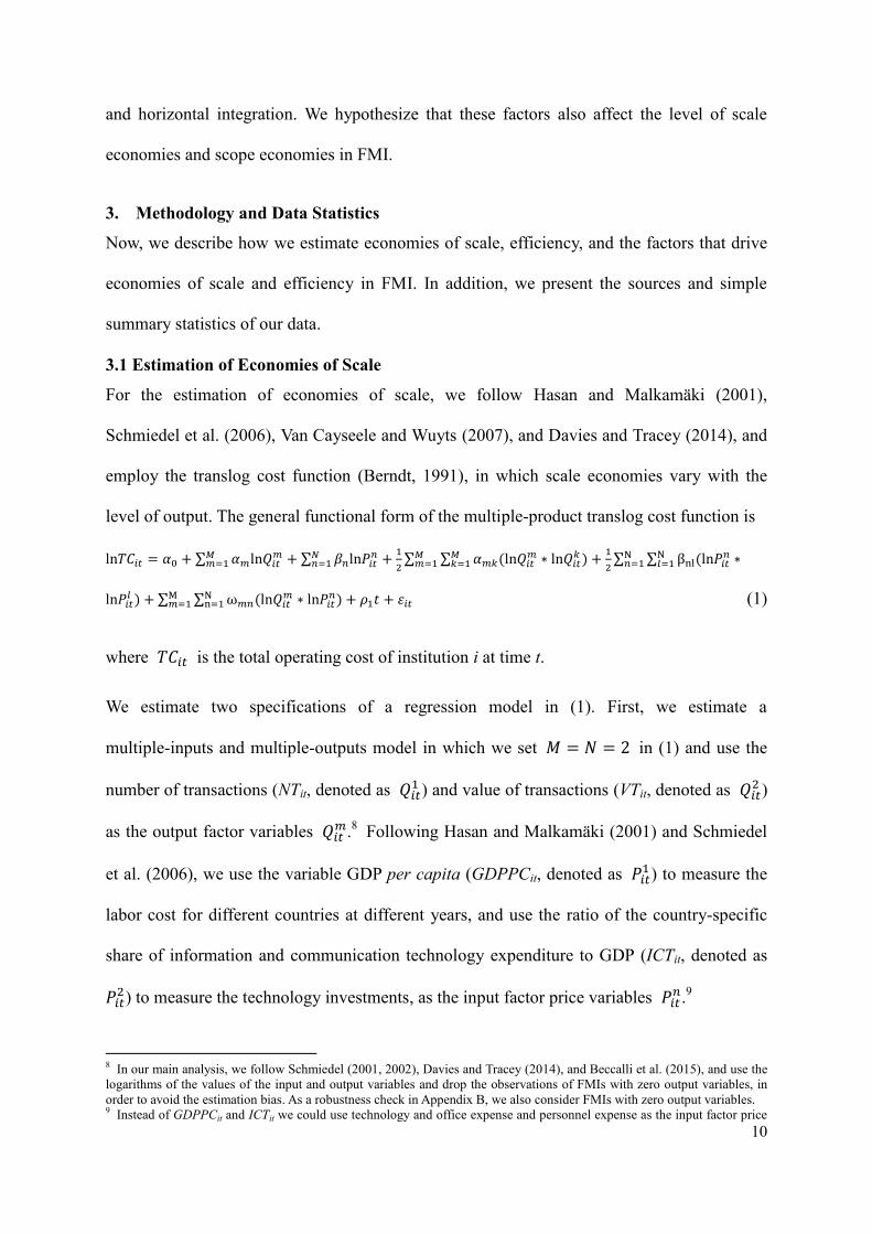
employ the translog cost function (Berndt, 1991), in which scale economies vary with the

level of output. The general functional form of the multiple-product translog cost function is

ln𝑇𝐶𝑖𝑡 = 𝛼0 + ∑ 𝛼𝑚ln𝑄𝑖𝑡𝑚𝑀

𝑚=1 + ∑ 𝛽𝑛ln𝑃𝑖𝑡𝑛𝑁

𝑛=1 +1

2∑ ∑ 𝛼𝑚𝑘(ln𝑄𝑖𝑡

𝑚 ∗ ln𝑄𝑖𝑡𝑘𝑀

𝑘=1𝑀𝑚=1 ) +

1

2∑ ∑ βnl(ln𝑃𝑖𝑡

𝑛 ∗N𝑙=1

N𝑛=1

ln𝑃𝑖𝑡𝑙 ) + ∑ ∑ ω𝑚𝑛(ln𝑄𝑖𝑡

𝑚 ∗ ln𝑃𝑖𝑡𝑛N

n=1M𝑚=1 ) + 𝜌1𝑡 + 𝜀𝑖𝑡 (1)

where 𝑇𝐶𝑖𝑡 is the total operating cost of institution i at time t.

We estimate two specifications of a regression model in (1). First, we estimate a

multiple-inputs and multiple-outputs model in which we set 𝑀 = 𝑁 = 2 in (1) and use the

number of transactions (NTit, denoted as 𝑄𝑖𝑡1 ) and value of transactions (VTit, denoted as 𝑄𝑖𝑡

2 )

as the output factor variables 𝑄𝑖𝑡𝑚.

8 Following Hasan and Malkamäki (2001) and Schmiedel

et al. (2006), we use the variable GDP per capita (GDPPCit, denoted as 𝑃𝑖𝑡1 ) to measure the

labor cost for different countries at different years, and use the ratio of the country-specific

share of information and communication technology expenditure to GDP (ICTit, denoted as

𝑃𝑖𝑡2) to measure the technology investments, as the input factor price variables 𝑃𝑖𝑡

𝑛.9

8 In our main analysis, we follow Schmiedel (2001, 2002), Davies and Tracey (2014), and Beccalli et al. (2015), and use the

logarithms of the values of the input and output variables and drop the observations of FMIs with zero output variables, in

order to avoid the estimation bias. As a robustness check in Appendix B, we also consider FMIs with zero output variables. 9 Instead of GDPPCit and ICTit we could use technology and office expense and personnel expense as the input factor price

11

We include the time trend variable t to control for technology development (see also Hou,

Wang, and Li, 2015). We estimate the translog cost function in (1) by employing both the

fixed effect estimation and stochastic frontiers analysis (SFA). The robust standard errors are

clustered at the firm level (see Appendix for details). Cost scale elasticities are calculated as

𝑒𝑄1(𝑄𝑖𝑡1 , 𝑄𝑖𝑡

2 ) =𝜕ln𝑇𝐶

𝜕ln𝑄1 = 𝛼1 + 𝛼11ln𝑄𝑖𝑡1 + 𝛼12ln𝑄𝑖𝑡

2 + ∑ 𝜔1𝑛ln𝑃𝑖𝑡𝑛2

n=1 (2)

𝑒𝑄2(𝑄𝑖𝑡1 , 𝑄𝑖𝑡

2 ) =𝜕ln𝑇𝐶

𝜕ln𝑄2= 𝛼2 + 𝛼22ln𝑄𝑖𝑡

2 + 𝛼12ln𝑄𝑖𝑡1 + ∑ 𝜔2𝑛ln𝑃𝑖𝑡

𝑛2n=1 (3)

where regression coefficients 𝛼𝑖 , 𝛼𝑚𝑘 , and 𝜔𝑚𝑛 are obtained from multiple-inputs and

multiple-outputs specification of (1) with 𝑀 = 𝑁 = 2. The inverse function of economies of

scale 𝐸𝑆2𝑖𝑡 at point (𝑄1, 𝑄2) of the output set is computed by the sum of the cost scale

elasticities with respect to both outputs

1

𝐸𝑆2𝑖𝑡= ∑

𝜕ln𝑇𝐶

𝜕ln𝑄𝑚2𝑚=1 = 𝑒𝑄1(𝑄𝑖𝑡

1 , 𝑄𝑖𝑡2 ) + 𝑒𝑄2(𝑄𝑖𝑡

1 , 𝑄𝑖𝑡2 ) (4)

Second, we estimate a single-input and single-output model in which we set 𝑀 = 𝑁 = 1 in

(1) and use the number of transactions (NTit, denoted as 𝑄𝑖𝑡1 ) as a single output, and GDP per

capita (GDPPCit, denoted as 𝑃𝑖𝑡1) as a single input. The inverse function of economies of

scale 𝐸𝑆1𝑖𝑡 at point 𝑄1 of the output set is computed by the cost scale elasticity with

respect to the single input

1

𝐸𝑆1𝑖𝑡=

𝜕ln𝑇𝐶

𝜕ln𝑄1= 𝛼1 + 𝛼11ln𝑄𝑖𝑡

1 + 𝜔11ln𝑃𝑖𝑡1 (5)

where regression coefficients 𝛼1 , 𝛼11 , and 𝜔11 are obtained from single-input and

single-output specification of (1) with 𝑀 = 𝑁 = 1.

3.2 Estimation of Efficiency

We also apply the frontier analysis by using DEA (following Cooper et al., 2004; Cummins et

variables. However, FMI frequently do not report these data. As a robustness check, we include variable STAFFit (denoted as

𝑃𝑖𝑡3), which is defined as the ratio of personnel expenses divided by the total assets, as another measure of labor cost. In

addition, we focus on the subsample of FMI that reports the value of personnel expense. The results remain qualitatively the

same (see Table A3 in the Appendix).

12

al., 2010) to estimate technical, cost, revenue, and profit efficiency for each firm in our

sample.10

Efficiency scores range between 0 and 1, where a value of 1 indicates that firms

are fully efficient, and values smaller than 1 indicate that firms are not fully efficient.

The technical efficiency (TEit) of a given firm is defined as the ratio of the input usage of a

fully efficient firm producing the same output vector as the given firm to the input usage of

the given firm. Technical efficiency (TEit) is a product of two parts: pure technical efficiency

(PTEit), which measures the efficiency relative to the variable returns to scale frontier, and

scale efficiency (SEit), which measures the distance between the variable returns to scale

frontier and the constant returns to scale frontier.

Cost efficiency is defined as the ratio of the costs of a fully efficient firm with the same

output quantities and input prices of a given firm to the given firm’s actual costs. Cost

efficiency can be decomposed into technical efficiency (TEit) and allocative efficiency (AEit),

which describes how well the firm chooses the optimal mix of inputs. Cost efficiency relative

to the constant returns to scale (CEit) is defined as the product of pure technical, scale, and

allocative efficiency, CEit = PTEit * SEit * AEit. We also estimate the cost efficiency under

variable returns to scale (VCEit) and cost efficiency under constant returns to scale purged of

scale efficiency (CEScopeit, defined as CEScopeit = CEit / SEit = PTEit * AEit).

Revenue efficiency is defined as the ratio of the revenues of a given firm to the revenue of a

fully efficient firm with the same input vector and output prices. We estimate the revenue

efficiency under both constant returns to scale (REit) and variable returns to scale (VREit). We

also estimate revenue efficiency under constant returns to scale purged of scale efficiency

(REScopeit, defined as REScopeit = REit / SEit). Finally, profit efficiency (PEit) is defined as

10 Alternatively, we could employ stochastic frontier analysis (e.g., as in Fang, Hasan, and Marton, 2011). We prefer DEA

because it avoids potential specification errors that can occur due to the improper specification of cost or revenue function.

DEA is also computed for an individual firm and does not require distributional assumptions.

13

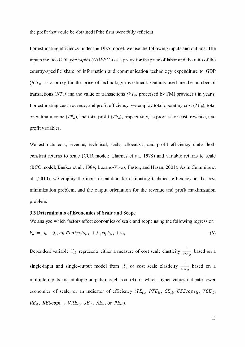
the profit that could be obtained if the firm were fully efficient.

For estimating efficiency under the DEA model, we use the following inputs and outputs. The

inputs include GDP per capita (GDPPCit) as a proxy for the price of labor and the ratio of the

country-specific share of information and communication technology expenditure to GDP

(ICTit) as a proxy for the price of technology investment. Outputs used are the number of

transactions (NTit) and the value of transactions (VTit) processed by FMI provider i in year t.

For estimating cost, revenue, and profit efficiency, we employ total operating cost (TCit), total

operating income (TRit), and total profit (TPit), respectively, as proxies for cost, revenue, and

profit variables.

We estimate cost, revenue, technical, scale, allocative, and profit efficiency under both

constant returns to scale (CCR model; Charnes et al., 1978) and variable returns to scale

(BCC model; Banker et al., 1984; Lozano-Vivas, Pastor, and Hasan, 2001). As in Cummins et

al. (2010), we employ the input orientation for estimating technical efficiency in the cost

minimization problem, and the output orientation for the revenue and profit maximization

problem.

3.3 Determinants of Economies of Scale and Scope

We analyze which factors affect economies of scale and scope using the following regression

𝑌𝑖𝑡 = φ0 + ∑ φkk 𝐶𝑜𝑛𝑡𝑟𝑜𝑙𝑠𝑖𝑡𝑘 + ∑ φjj 𝐹𝑖𝑡𝑗 + ε𝑖𝑡 (6)

Dependent variable 𝑌𝑖𝑡 represents either a measure of cost scale elasticity 1

ES1𝑖𝑡 based on a

single-input and single-output model from (5) or cost scale elasticity 1

ES2𝑖𝑡 based on a

multiple-inputs and multiple-outputs model from (4), in which higher values indicate lower

economies of scale, or an indicator of efficiency (𝑇𝐸𝑖𝑡, 𝑃𝑇𝐸𝑖𝑡, 𝐶𝐸𝑖𝑡, 𝐶𝐸𝑆𝑐𝑜𝑝𝑒𝑖𝑡, 𝑉𝐶𝐸𝑖𝑡,

𝑅𝐸𝑖𝑡, 𝑅𝐸𝑆𝑐𝑜𝑝𝑒𝑖𝑡, 𝑉𝑅𝐸𝑖𝑡, 𝑆𝐸𝑖𝑡, 𝐴𝐸𝑖𝑡, or 𝑃𝐸𝑖𝑡).

14

We are interested in how several factors 𝐹𝑖𝑡𝑗 affect economies of scale and efficiency. We

analyze the effect of institution size (logarithm of total assets, denoted by Sizeit), the

institution type (Dummy clearing housei equals one if the FMI provider is a clearing house

and zero otherwise, and Dummy CSDi equals one if the FMI provider is a CSD and zero

otherwise), the effects of horizontal mergers between the same types of institutions

(Horizontally integratedit), and the effects of vertical mergers between different types of

institutions (Vertically integratedit). More specifically, the dummy variable Vertically

integratedit equals one if the FMI provider is or has become vertically integrated with another

FMI provider (i.e., if a clearing house or CSD is vertically integrated with a stock exchange)

and zero otherwise. The dummy variable Horizontally integratedit equals one from the year

the FMI provider merged with the same type of FMI provider onwards, and zero otherwise.

We also analyze the impact of the geographic location (Dummy North Americai, Dummy

Europei, and Dummy Asia-Pacifici), and the degree of specialization of the FMI providers

(Broad range of asset classesi) on the economies of scales and efficiency measures. The

dummy variable Broad range of asset classesi equals zero if the FMI provider offers services

only for bonds and equities securities, and equals one if the FMI provider also offers services

for other instruments such as derivatives and commodities.

As control variables 𝐶𝑜𝑛𝑡𝑟𝑜𝑙𝑠𝑖𝑡𝑘, we include GDP growthit and Inflationit in a country to

account for the changes of economic cycles. We also add Interest ratesit and Stocks trade

ratioit, defined as the value of stocks traded to GDP, to control for the changes in monetary

policy and the size of the security market in a given country. To control for the risk-taking of

the institutions, we follow Hughes and Mester (1993) and include the logarithm of equity to

asset ratio, denoted as ln EOAit. In an additional specification, we also include the logarithm

of ICTit and a time trend t to capture the effect of technological development. The definitions

15

of the variables are presented in Table 1. We estimate the regression in (6) by using the

feasible generalized least squares (FGLS). To deal with residuals that may be correlated

across time we include dummy variables for each time period and then estimate standard

errors allowing for heteroscedastic standard errors in firm dimension.

3.4 Data Collection

We collect the data from several sources. The financial information of CSDs and clearing

houses was collected from the Bankscope database and annual reports, and the data for stock

exchanges was acquired from annual reports. The data for the total number and value of

transactions for clearing houses and CSDs are obtained from Bank for International

Settlement Statistics on Payment and Settlement Systems, and data for stock exchanges are

collected from the World Federation of Exchanges Annual Yearbooks. Macroeconomic data

are taken from the IMF International Financial Statistics (IFS) and the World Bank Database.

The information on merger and acquisition activities is obtained from the Zephyr database.

All of the data were collected in national currencies, converted into US dollars and

inflation-adjusted. Table 1 lists data sources per each variable.

Our sample consists of eighty-two institutions, including thirty stock exchanges, twenty-nine

clearing houses, and twenty-three CSDs, amounting to 653 firm-year observations, from

regions including Europe, North America, the Asia-Pacific region, South America, and

Africa between 2000 and 2015. Table A4 in Appendix lists the FMI providers in our data and

their institutional characteristics.

<Insert Table 1 here>

3.5 Data Statistics

Table 2 provides descriptive statistics. The average values of total operating cost and total

operating income are $256.9 million and $348.9 million, respectively. Regarding the output

variables, the average number of transactions per institution per year is 1.306 billion and the

16

average total value of the transactions per institution per year is $66.620 trillion. Regarding

the input variables, the average value of GDPPC is $32,200, the average ICT is 1.66%, and

the average value of personnel expense per institution per year is $78.8 million. The average

value of equity to total assets, EOA, is 31.5%.


Based on the type of FMI provider, we can split our sample into subsamples of stock

exchanges, clearing houses, and CSDs. Even though clearing houses are the biggest in terms

of average total assets (stock exchanges have medium assets and CSDs have the smallest total

assets), they generate the lowest total operating cost and operating income (followed by the

CSDs and the stock exchanges). The average number and value of transactions per institution

per year are the highest for clearing houses, followed by CSDs, and the lowest for stock

exchanges. Clearing houses are also the most leveraged among the FMI providers (with EOA

of only 7.93%), followed by CSDs (with EOA of 27.37%) and stock exchanges (with EOA of

52.58%). Clearing houses incur the lowest personnel expenses, followed by stock exchanges

and CSDs.

We also divide our sample based on specialization. FMI providers that focus on a broad range

of asset classes have higher operating costs, operating income, personnel expenses, and total

assets, but a lower number and value of transactions than FMI providers that focus on a

narrow range of asset classes.

Finally, we split our sample according to different types of integration. The results show that

horizontally integrated FMI providers have higher operating costs, operating income, and

personnel expenses, but lower total assets, and a lower number and value of transactions than

non-horizontally integrated FMI providers. Vertically integrated FMI providers have not only

higher operating costs, operating income, and personnel expenses, but also a higher number

17

and value of transactions than non-vertically integrated FMI providers.

4. Empirical Results

In this section, we first present the main performance indicators of the FMI providers. Second,

we perform the translog analysis and estimate the economies of scale in FMI. Third, we

employ DEA to estimate efficiency scores and analyze economies of scope in FMI.

4.1 Simple Performance Indicators

We overview several simple performance indicators of the total sample, CSDs, stock

exchanges, and clearing houses from Europe, North America, the Asia-Pacific region, and

South America and Africa in Table 3. Table 3 also provides the performance ratios of the

subsamples based on the institution size, specialization, and type of integration. We can

observe that the performance indicators vary considerably across the size, type of institution,

geographic location, specialization, and type of integration.


As an indicator of cost efficiency, we compute cost per trade, defined as the total operating

cost divided by number of transactions, TC/NT. It represents an estimate of the average unit

cost of settling a trade in the market. The average TC/NT is $423.77 for CSDs, $63.16 for

stock exchanges, and $38.71 for clearing houses. Another variable that discerns cost

efficiency is the cost per value of transaction, TC/VT. Stock exchanges exhibit the highest

TC/VT, with an average TC/VT of $0.0033, followed by CSDs, with an average TC/VT of

$0.0007, and clearing houses, with the lowest average TC/VT of $0.000009. As a profitability

indicator, we compute operating income per trade, TR/NT, and operating income per value of

transaction, TR/VT. The average TR/NT of CSDs is the highest and is around three times that

of TR/NT of stock exchanges, and twelve times that of TR/NT of clearing houses. The average

TR/VT is the highest for stock exchanges, followed by CSDs and clearing houses.

18

We are interested in how the size of an FMI affects simple cost performance indicators. The

average TC/NT and TR/NT is much higher for large FMI providers than for small ones. To

understand this, note that large FMI providers in our sample include the NASDAQ, New

York Stock Exchange, TMX Group, Deutsche Boerse, London Stock Exchange, Euroclear

Bank, Clearstream International, the Depository Trust Company, and Tokyo Stock Exchange.

Most of them provide cross-border services, which are generally costlier than domestic

transactions (see Giovannini Group, 2002; De Carvalho, 2004; Schmiedel and Schönenberger,

2005). In contrast, the largest FMI providers have a much lower value of TC/VT and TR/VT

compared to the smallest ones, potentially because they process most of the high-value

transactions.

We graphically depict the relationship between the number of transactions and TC/NT in

Figure 1 and the relationship between the value of transactions and TC/VT in Figure 2. Figure

1 and Figure 2 indicate that, with the increasing number of transactions and the value of

transactions, the cost per trade and the cost per value of transaction are decreasing. These

findings persist across the subsamples of clearing houses, CSDs, and stock exchanges,

indicating that simple cost performance indicators improve with the size of FMI.

<Insert Figure 1 & Figure 2 here>

Comparison across regions reveals that the average TC/NT, TC/VT, TR/NT, and TR/VT in

North America are the lowest compared to other regions, consistent with the view of Lannoo

and Levin (2002), Giovannini Group (2002, 2003), Hasan et al. (2003), and Schmiedel et al.

(2006) that FMI providers in North America are highly efficient and operate in a highly

competitive environment. The average VT/NT in North America is $267.2 million, which is

higher compared to other regions. A potential explanation is that FMI providers from North

America offer services to larger and more international firms with a higher average value of

19

transaction.

We also check whether performance indicators vary with horizontal and vertical integration,

and with a focus on a broad versus narrow range of asset classes. Horizontally integrated FMI

providers have lower TC/NT, TR/NT, and TR/VT than non-horizontally integrated FMI

providers. Vertically integrated FMI providers have higher TC/NT and TR/NT and lower

TR/NT and TR/VT than non-vertically integrated FMI providers. The FMI that provide

services for a broad range of asset classes also have significantly higher TC/NT and TR/NT

and lower TR/NT and TR/VT than FMI that focus on a narrow range of asset classes.

4.2 Economies of Scale

We now estimate whether economies of scale exist in FMI. We apply the single-input and

single-output model in (5) and multiple-inputs and multiple-outputs model in (4) for our total

sample and for various subsamples.11

Following Hughes and Mester (2013), we compute the

mean of cost scale elasticities for the total sample and various subsamples (see Panel A and

Panel B in Table 4, respectively). The results in each panel are reported based on size,

horizontal and vertical integration, type of FMI, geographical location, and specialization. In

the case of a single input and a single output model, the mean cost scale elasticity of the total

sample with respect to the number of transactions is 0.0889. This indicates that the operating

cost increases by 8.89% if the number of transactions is doubled.

The mean cost scale elasticity based on the multiple-inputs and multiple-outputs model with

respect to the number of transactions is 0.155 (Panel B in Table 4). This indicates that the

operating cost would increase by 15.5% if the number of transactions were doubled. The

mean cost scale elasticity with respect to the value of transactions is 0.0604, meaning that the

operating cost would increase by 6.04% if the value of transactions were doubled. The

11 We derive the value of economies of scale (see (4) and (5)) from the coefficients estimated in column (6) of Panel A and

Panel B in Table A2, respectively.

20

operating cost increases by 21.54% if both outputs are doubled.12

These findings confirm the

existence of economies of scale in the FMI.


In order to test the impact of institution size on the economies of scale of the FMI, we divide

our sample into four subsamples based on the total assets, and estimate the cost scale

elasticities of four different subsamples. The results indicate that the economies of scale are

higher for large institutions than for small ones. If the number (value) of transactions is

doubled, the operating cost increases by 25.06% (10.76%) for the smallest institutions in the

first quantile, but only by 8.79% (6.07%) for the largest ones in the fourth quantile.

Table 4 shows that the economies of scale are higher if FMI providers are vertically or

horizontally integrated. Results of the single-input and single-output model (see Panel A of

Table 4) show that operating costs of vertically integrated FMI providers increase by 7.6% if

the number of transactions is doubled, compared to 9.27% for FMI providers that are not

vertically integrated. Results of the multiple-inputs and multiple-outputs model (see Panel B

of Table 4) show that operating costs of vertically integrated FMI providers increase by 16.30%

if both outputs are doubled, compared to 23.84% for FMI providers that are not vertically

integrated. The results of horizontal integration are similar. This confirms that vertical and

horizontal integration within FMI is associated with higher economies of scale and

corroborates previous evidence in Tapking and Yang (2006).

We confirm that economies of scale exist within different types of FMI (i.e., clearing houses,

CSDs, and stock exchanges). Doubling the number of transactions increases the operating

cost by 8.35% (16.95%) for clearing houses, 7.46% (19.13%) for CSDs, and 10.39% (23.83%)

for stock exchanges, as predicted by the single-input and single-output model

12 Instead of the translog model in (1), we also use the loglinear model with qualitatively similar results (see Appendix,

Table A1).

21

(multiple-inputs and multiple-outputs model). Our results indicate that economies of scale are

the highest for clearing houses, lower for CSDs, and the lowest for stock exchanges.

Larger FMI providers (the top 50% in total assets) realize higher economies of scale than

smaller ones (the bottom 50% in total assets). This is confirmed across the total sample and

within the subsamples of clearing houses, CSDs, and stock exchanges.

Our findings confirm the existence of economies of scale in each regional subsample. A

substantial variation in the degree of economies of scale exists across regions. The economies

of scale are the highest in North America and the lowest in South America and Africa. The

doubling of the outputs increases costs by 6.07% and 14.35%, as predicted by the

single-input and single-output model for North America and for South America and Africa,

respectively (and by 13.47% and 43.73% as predicted by the multiple-inputs and

multiple-outputs model).

We also separate FMI based on their specialization. Doubling the outputs results in a lower

cost increase for FMI providers that offer services for a broad range of asset classes compared

to FMI providers that offer services for a narrow range of asset classes.

4.3 Efficiency Scores

We perform DEA estimation on the total sample that includes stock exchanges, CSDs, and

clearing houses, and we estimate average technical efficiency (TEit), pure technical efficiency

(PTEit), cost efficiency (CEit), cost efficiency purged of scale efficiency (CEScopeit), cost

efficiency based on variable returns to scale technology (VCEit), revenue efficiency (REit),

revenue efficiency purged of scale efficiency (REScopeit), revenue efficiency based on

variable returns to scale technology (VREit), input-oriented scale efficiency (SEit),

input-oriented allocative efficiency (AEit), and profit efficiency (PEit); see Table 5.

22

Clearing houses on average have higher technical, cost, revenue, scale, and profit efficiency

than stock exchanges and CSDs. Cost efficiency under constant returns to scale (variable

returns to scale) averages 34.18% (46.72%) for clearing houses, 5.92% (16.66%) for stock

exchanges, and 4.13% (12.91%) for CSDs. Revenue efficiency under constant returns to scale

(variable returns to scale) averages 17.95% (24.13%) for clearing houses, 2.43% (9.23%) for

stock exchanges, and 3.97% (4.03%) for CSDs.


Revenue, scale, and profit efficiency are significantly higher, whereas technical and cost

efficiency are significantly lower for large FMI providers (the top 50% in total assets) than

for small FMI providers (the bottom 50% in total assets). This indicates that economies of

scale in FMI stem from revenue, scale, and profit efficiency rather than from technical and

cost efficiency.

We also analyze how horizontal and vertical integration affect the efficiency of FMI

providers. Horizontal integration is associated with significantly decreased technical

efficiency, cost, revenue, scale, and profit efficiency, whereas vertical integration is

associated with significantly increased pure technical, revenue, and profit efficiency. A

negative relationship between horizontal integration and efficiency indicators and a positive

relationship between vertical integration and efficiency indicators also persists across

subsamples of stock exchanges, CSDs, and clearing houses.

FMI providers that focus on a broad range of asset classes operate less efficiently than FMI

providers that focus on a narrow range of asset classes.

The results of returns to scale are presented in Panel B in Table 5. None of the stock

exchanges, and only 2.1% of CSDs and 7.7% of clearing houses, operate under constant

returns to scale. All three types of institutions are more likely to operate under increasing

23

returns to scale than under decreasing returns to scale, supporting the presence of economies

of scale in FMI.

5. Multiple Regression Analysis

5.1 Factors Affecting Economies of Scale

We now analyze the factors that affect the economies of scale in FMI using the single-input

and single-output model in (5) and the multiple-inputs and multiple-outputs model in (4) to

estimate cost scale elasticities; see Table 6.


Dummy clearing housei and Dummy CSDi are negatively and significantly related to cost

scale elasticity. The absolute value of the regression coefficient of Dummy CSDi is smaller

than the regression coefficient of Dummy clearing housei. This provides some evidence that

the economies of scale for clearing houses (and to a smaller level also for CSDs) are

significantly higher than the economies of scale for stock exchanges.

We find that the size of FMI providers is negatively associated with cost scale elasticity,

indicating that economies of scale increase with the institution size. The dummy variable

Horizontally integratedit is negatively related to cost scale elasticity, showing that the

economies of scale are positively related to horizontal integration. The dummy variable

Vertically integratedit is negatively related to cost scale elasticity, indicating that the

economies of scale are positively related to vertical integration.

The negative sign of the regression coefficient of Broad range of asset classesi confirms that

the FMI providers that offer services for a broad range of asset classes have higher economies

of scale than the ones that only focus on a narrow range of asset classes.

We also find that the dummy variables Dummy Europei and Dummy Asia-Pacifici are

positively related to cost scale elasticity, and Dummy North Americai is negatively related to

24

cost scale elasticity. This indicates that economies of scale are lower in Europe and the

Asia-Pacific region and higher in North America compared to other regions.

Variable ICTit is negatively and statistically significantly related to cost scale elasticity. This

is consistent with the view that with the technological development is positively associated

with economies of scale in financial institutions (see Boot, 2014; Hasan et al., 2003; Knieps,

2006; Marinč, 2013).

To conclude, economies of scale increase with size and with horizontal and vertical

integration. Clearing houses (and CSDs) have higher economies of scale than stock

exchanges. Economies of scale are significantly higher in North America than in other

regions. The FMI providers that provide services for a broad range of asset classes can

exploit higher economies of scales. Technological development is positively related to the

economies of scale in FMI.

5.2 Factors Affecting Efficiency Scores

We now analyze factors that affect efficiency scores using the regression analysis in (6). We

find that large FMI providers have significantly higher revenue efficiency but lower cost,

scale, and allocative efficiency than smaller FMI providers. See Table 7.


Vertical integration is positively associated with pure technical and cost efficiency, whereas

horizontal integration is negatively associated with pure technical and cost efficiency.

Technical, cost, revenue, and profit efficiency are significantly higher for clearing houses

than for stock exchanges and CSDs. FMI providers in North America have higher allocative

efficiency but lower technical, revenue, and scale, and profit efficiency than FMI providers in

other regions. One explanation is that FMI from North America provide transaction services

25

with high volume and values, but with lower cost and revenue, and they are largely engaged

in cross-border trading.

FMI providers that focus on a broad range of asset classes have significantly lower technical

and cost efficiency than FMI providers that focus on a narrow range of asset classes.

Focusing on cost and revenue efficiency purged of scale efficiency effects (CEScopeit and

REScopeit), we can confirm that large FMI providers have significantly lower CEScopeit but

higher REScopeit than smaller FMI providers. CEScopeit is positively associated with vertical

integration and negatively with horizontal integration. Clearing houses have significantly

higher CEScopeit and REScopeit than stock exchanges. FMI in Europe have significantly

lower REScopeit and CEScopeit compared to other regions.

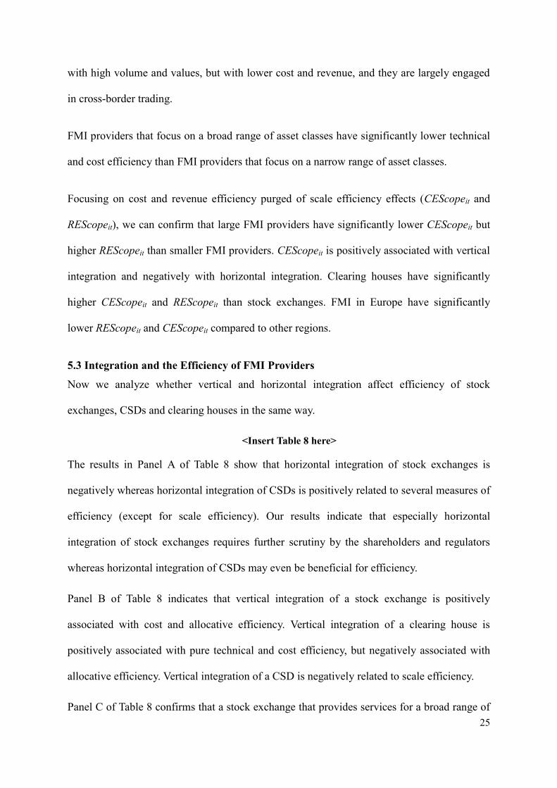
5.3 Integration and the Efficiency of FMI Providers

Now we analyze whether vertical and horizontal integration affect efficiency of stock

exchanges, CSDs and clearing houses in the same way.


The results in Panel A of Table 8 show that horizontal integration of stock exchanges is

negatively whereas horizontal integration of CSDs is positively related to several measures of

efficiency (except for scale efficiency). Our results indicate that especially horizontal

integration of stock exchanges requires further scrutiny by the shareholders and regulators

whereas horizontal integration of CSDs may even be beneficial for efficiency.

Panel B of Table 8 indicates that vertical integration of a stock exchange is positively

associated with cost and allocative efficiency. Vertical integration of a clearing house is

positively associated with pure technical and cost efficiency, but negatively associated with

allocative efficiency. Vertical integration of a CSD is negatively related to scale efficiency.

Panel C of Table 8 confirms that a stock exchange that provides services for a broad range of

26

asset classes has lower technical, pure technical, and cost efficiency. A clearing house that

provides services for a broad range of asset classes has lower technical, pure technical, cost,

revenue, and profit efficiency, but higher scale and allocative efficiency. A CSD that provides

services for a broad range of asset classes has higher revenue and allocative efficiency.

5.4 Efficiency of FMI providers and Systemic Risk

Now we analyze whether the efficiency of the FMI providers is associated with the systemic

risk in the financial system. We use different measures of systemic risk. As a measure of the

financial distress of the banking sectors, we use the variable NPL, which is defined as the

bank non-performing loans to total gross loans in a financial system. As a measure of

systemic risk of the stock market, we use the variable Stock Market Index Volatility, which is

defined as the volatility of the stock market index return for each country at each year and

calculated based on the monthly returns of the stock market index. To measure the systemic

risk in the EU countries, we employ the variable Country-Level Index of Financial Stress

(CLIFS), which is defined as a measure of financial stress in Duprey et al. (2015) and Duprey

and Klaus (2017).

Following Levine et al. (2000), Laeven (2003), Carlin and Mayer (2003), and Cecchetti and

Kharroubi (2012), we include GDP growth and Inflation in each country at each year as

control variables to account for economic cycle. Interest rate and Number of FMIs control for

the changes of monetary policy and the industry structure of the FMIs in a given country. ICT

controls for the changes of technology development. We also include variable Private credit

by banks to GDP to control for the financial sector size. We employ the feasible generalized

least squares (FGLS) estimator to cope with potential heteroskedasticity problems and

include the yearly dummies to control the time fixed effects. See Table 9.


The results in Table 9 indicate that revenue efficiency is negatively and significantly

27

associated with the non-performing loan ratio (NPL) whereas cost efficiency is positively

related to NPL. Increasing revenue efficiency and decreasing cost efficiency of the FMI

providers may be associated with higher stability of the banking system.

Table 9 shows that efficiency measures of FMI providers are not statistically significantly

related to Stock Market Index Volatility, which is used as a measure of the stock market

financial distress.

Table 9 also shows that pure technical efficiency and revenue efficiency are negatively

associated with Country-Level Index of Financial Stress (CLIFS), which is used as a measure

of a systemic risk in the financial systems.13

In sum, we find some support for the relationship between the efficiency measures of FMI

providers and systemic risk. However, the relationships are only weakly significant and no

causality is established. Further analysis is needed to support our results.

5.5 Integrations of FMI Providers, Systemic Risk, and Financial Development

We are also interested whether the form of integration between FMI providers is related to the

systemic risk within the financial system. We employ the variables, including NPL, Stock

Market Index Volatility, and Country-Level Index of Financial Stress (CLIFS), as measures of

financial distress of financial system. We follow Cecchetti and Kharroubi (2012) and use two

different measures: Stock Market Capitalization Ratio, which is defined as the ratio of market

capitalization of listed companies to GDP, and Banking System Asset to GDP Ratio, which is

defined as the banking system asset to GDP ratio, as the measures of stock market and

banking system development.

We include the variables Size, Broad range of asset classes, Dummy clearing house, Dummy

CSD, Dummy Europe, Dummy North America, and Dummy Asia-Pacific to control for the

13

As the data of Country-Level Index of Financial Stress (CLIFS) is only available for EU countries, we only perform our

analysis on the subsample of EU countries.

28

firm-level characteristics. We also include a set of control variables including GDP growth,

Inflation rate, Interest rate, ICT, and ln EOA, and employ the feasible generalized least

squares (FGLS) estimator to cope with potential heteroskedasticity problems. Year dummies

are also included to control the time fixed effects. See Table 10.


Columns (1)–(3) in Table 10 show that vertical and horizontal integration are negatively and

significantly associated with non-performing loan ratio (NPL).14

Columns (4)-(5) show that

vertical integration is positively and significantly related to Banking System Asset to GDP

ratio, and horizontal integration is positively and significantly associated with both Stock

Market Capitalization Ratio and Banking System Asset to GDP ratio. Broad range of asset

classes is positively and significantly related to the measures of systemic risk (NPL, Stock

Market Index Volatility, and CLIFS) and to the measures of financial system development

(Banking System Asset to GDP ratio and Banking System Asset to GDP ratio).

Hence, horizontal and vertical integration as well as broad orientation of FMI providers (that

offer services for broad range of asset classes) is associated with several measures of

systemic risk and financial system development.

6. Conclusion

In this article we analyze economies of scale and scope within FMI, based on the panel data

of thirty stock exchanges, twenty-nine clearing houses, and twenty-three CSDs from

thirty-six countries. We investigate the impact of size, horizontal and vertical integration,

type, focus on a narrow versus broad range of asset classes, and geographic location on

economies of scale and scope.

We confirm the existence of economies of scale in FMI. Economies of scale are positively

14

Dummy variables Dummy Europe, Dummy North America, and Dummy Asia-Pacific are dropped out of the regression in

column (3) in Table 10 because of the data of CLIFS is only available for EU countries.

29

associated with size, horizontal and vertical integration of an FMI provider, and its focus on a

broad range of asset classes, and are the highest in North America and Europe. This indicates

that the best strategy for large, horizontally and vertically integrated FMI providers is to

focus further on high growth and reap the benefits of economies of scale.

Our findings also suggest that economies of scale mostly derive from the improvements in

revenue efficiency and profit efficiency rather than cost efficiency. A potential explanation is

that larger FMI providers offer higher quality products and services that raise costs but also

raise revenues by more than the cost increases; this is consistent with evidence in the banking

industry (see Berger and Mester, 2003).

We find that the efficiency of FMI providers is positively related to vertical integration but

negatively to horizontal integration and to the focus on a broad range of asset classes.

Therefore, economies of scope seem to be present in vertical integration of clearing houses

and CSDs with stock exchanges but not in horizontal integration across the FMI providers of

equal types, nor in the combination of services provided for a broad range of asset classes.

30

References

Acharya, V., and Bisin, A. (2014). Counterparty risk externality: Centralized versus

over-the-counter markets. Journal of Economic Theory, 149, 153-182.

Acharya, V. V., Hasan, I., and Saunders, A. (2006). Should Banks Be Diversified? Evidence

from Individual Bank Loan Portfolios. Journal of Business, 79(3), 1355–1412.

Banker, R. D., Charnes, A., and Cooper, W. W. (1984). Some Models for Estimating

Technical and Scale Inefficiencies in Data Envelopment Analysis. Management

Science, 30(9), 1078–1092.

Beccalli, E., Anolli, M., and Borello, G. (2015). Are European banks too big? Evidence on

economies of scale. Journal of Banking & Finance, 58, 232-246. doi:

http://dx.doi.org/10.1016/j.jbankfin.2015.04.014.

Beijnen, C., and Bolt, W. (2009). Size matters: Economies of scale in European payments

processing. Journal of Banking & Finance, 33(2), 203-210.

Berger, A. N., Hasan, I., Zhou, M. (2010). The Effects of Focus Versus Diversification on

Bank Performance: Evidence from Chinese Banks. Journal of Banking & Finance,

34(7), 1417–1435.

Berger, A. N., and Mester, L. J. (2003). Explaining the Dramatic Changes in Performance of

US Banks: Technological Change, Deregulation, and Dynamic Changes in

Competition. Journal of Financial Intermediation, 12(1), 57–95.

Bernanke, B. S. (1990). Clearing and Settlement during the Crash. Review of Financial

Studies, 3(1), 133–151.

Berndt, E. (1991). The Practice of Econometrics: Classic and Contemporary. Cambridge,

MA: Massachusetts Institute of Technology and the National Bureau of Economic

Research; Reading, MA: Addison-Wesley Publishing Company, Inc.

Boot, A. W. A. (2014). Financial Sector in Flux. Journal of Money, Credit and Banking, 46(1),

129–135.

Boot, A. W. A. (2016). Understanding the Future of Banking: Scale & Scope Economies, and

Fintech, in The Future of Large Internationally Active Banks (A. Demirgüç-Kunt, D.D.

Evanoff, and G. Kaufmann, eds.). World Scientific Studies in International Economics,

55, pp. 429–448.

Carlin, W., and Mayer, C. (2003). Finance, investment, and growth. Journal of Financial

Economics, 69(1), 191-226.

Cecchetti, S. G., and Kharroubi, E. (2012). Reassessing the Impact of Finance on Growth.

http://dx.doi.org/10.1016/j.jbankfin.2015.04.014

31

BIS Working Papers.

Charles, A., Darné, O., Kim, J. H., and Redor, E. (2016). Stock Exchange Mergers and

Market Efficiency. Applied Economics, 48(7), 576–589. doi:

10.1080/00036846.2015.1083090.

Charnes, A., Cooper, W. W., and Rhodes, E. (1978). Measuring the Efficiency of Decision

Making Units. European Journal of Operational Research, 2(6), 429–444.

Cherbonnier, F., and Rochet, J.-C. (2010). Vertical Integration and Regulation in the

Securities Settlement Industry. TSE Working Paper.

Choi, S., Francis, B. B., and Hasan, I. (2010). Cross-Border Bank M&As and Risk: Evidence

from the Bond Market. Journal of Money, Credit and Banking, 42, 615–645.

Cooper, W. W., Seiford, L. M., and Zhu, J. (2004). Data Envelopment Analysis. Boston:

Kluwer Academic.

Committee on Payment and Settlement Systems, Board of the International Organization of

Securities Commissions. (2012). Principles For Financial Market Infrastructure.

Bank for International Settlements, April 2012.

http://www.bis.org/cpmi/publ/d101a.pdf

Cummins, J. D., Weiss, M. A., Xie, X., and Zi, H. (2010). Economies of Scope in Financial

Services: A DEA Efficiency Analysis of the US Insurance Industry. Journal of

Banking & Finance, 34(7), 1525–1539.

Davies, R., and Tracey, B. (2014). Too Big to Be Efficient? The Impact of Implicit Subsidies

on Estimates of Scale Economies for Banks. Journal of Money, Credit and Banking,

46(s1), 219–253. doi: 10.1111/jmcb.12088

De Carvalho, C. (2004). Cross-Border Securities Clearing and Settlement Infrastructure in

the European Union as a Prerequisite to Financial Markets Integration: Challenges

and Perspectives. HWWA Discussion Paper no. 287.

Dicle, M. F., and Levendis, J. (2013). The Impact of Technological Improvements on

Developing Financial Markets: The Case of the Johannesburg Stock Exchange.

Review of Development Finance, 3(4), 204–213. doi:

http://dx.doi.org/10.1016/j.rdf.2013.09.001

Droll, T., Podlich, N., and Wedow, M. (2016). Out of Sight, Out of Mind? On the Risk of

Sub-Custodian Structures. Journal of Banking & Finance, 68, 47–56.

Duprey, T., and Klaus, B. (2017). How to Predict Financial Stress? An Assessment of Markov

Switching Models. ECB Working Paper No. 2057.

32

Duprey, T., Klaus, B., and Peltonen, T. (2015). Dating Systemic Financial Stress Episodes in

the EU Countries. ECB Working Paper No. 1873.

European Commission. (2015). Action Plan on Building a Capital Markets Union,

COM(2015) 468 final.

http://eur-lex.europa.eu/legal-content/EN/TXT/HTML/?uri=CELEX:52015DC0468&

from=EN

Fang, Y., Hasan, I., and Marton, K. (2011). Bank Efficiency in South-Eastern Europe.

Economics of Transition, 19, 495–520. doi:10.1111/j.1468-0351.2011.00420.x

Ferrarini, G., and Saguato, P. (2015). Regulating Financial Market Infrastructures. In E.

Ferran, N. Moloney, & J. Payne (eds.), The Oxford Handbook of Financial

Regulation, pp. 568–595. Oxford: Oxford University Press.

Francis, B. B., Hasan, I., and Sun, X. (2008). Financial Market Integration and the Value of

Global Diversification: Evidence for US Acquirers in Cross-Border Mergers and

Acquisitions. Journal of Banking & Finance, 32(8), 1522–1540.

Fu, X. M., Lin, Y. R., and Molyneux, P. (2014). Bank Competition and Financial Stability in

Asia Pacific. Journal of Banking & Finance, 38, 64–77.

Gehrig, T., and Stenbacka, R. (2007). Information Sharing and Lending Market Competition

with Switching Costs and Poaching. European Economic Review, 51(1), 77–99.

Giddy, I., Saunders, A., and Walter, I. (1996). Alternative Models for Clearance and

Settlement: The Case of the Single European Capital Market. Journal of Money,

Credit and Banking, 28(4), 986–1000.

Giovannini Group. (2002). Cross-Border Clearing and Settlement Arrangements in the

European Union. Brussels: Directorate-General for Economic and Financial Affairs,

European Commission.

Giovannini Group. (2003). Second Report on EU Clearing and Settlement Arrangements.

Brussels: Directorate-General for Economic and Financial Affairs, European

Commission.

Hasan, I., and Malkamäki, M. (2001). Are Expansions Cost Effective for Stock Exchanges? A

Global Perspective. Journal of Banking & Finance, 25(12), 2339–2366.

Hasan, I., Malkamäki, M., and Schmiedel, H. (2003). Technology, Automation, and

Productivity of Stock Exchanges: International Evidence. Journal of Banking &

Finance, 27(9), 1743–1773.

Hasan, I., and Schmiedel, H. (2004). Networks and Equity Market Integration: European

33

Evidence. International Review of Financial Analysis, 13(5), 601–619.

Hasan, I., Schmiedel, H., and Song, L. (2012a). Growth Strategies and Value Creation: What

Works Best for Stock Exchanges? Financial Review, 47(3), 469–499.

Hasan, I., Schmiedel, H., and Song, L. (2012b). How Stock Exchange Mergers and

Acquisitions Affect Competitors’ Shareholder Value: Global Evidence. In G. Poitras

(ed.), Handbook of Research on Stock Market Globalization, vol. 1, pp. 181–194.

Cheltenham, UK: Edward Elgar Publishing.

Heath, A., Kelly, G., Manning, M., Markose, S., and Shaghaghi, A. R. (2016). CCPs and

network stability in OTC derivatives markets. Journal of Financial Stability, 27,

217-233.

Holthausen, C., and Tapking, J. (2007). Raising Rival’s Costs in the Securities Settlement

Industry. Journal of Financial Intermediation, 16(1), 91–116.

Hou, X., Wang, Q., and Li, C. (2015). Role of Off-Balance Sheet Operations on Bank Scale

Economies: Evidence from China’s Banking Sector. Emerging Markets Review, 22,

140–153. doi: http://dx.doi.org/10.1016/j.ememar.2014.10.001

Hughes, J. P., and Mester, L. J. (1993). A Quality and Risk-Adjusted Cost Function for Banks:

Evidence on the “Too-Big-to-Fail” Doctrine. [journal article]. Journal of Productivity

Analysis, 4(3), 293–315. doi: 10.1007/bf01073414

Hughes, J. P., and Mester, L. J. (2013). Who Said Large Banks Don’t Experience Scale

Economies? Evidence from a Risk-Return-Driven Cost Function. Journal of

Financial Intermediation, 22(4), 559–585.

International Monetary Fund. (2009). Global Financial Stability Report, October 2009:

Navigating the Financial Challenges Ahead. 250.

Juranek, S., and Walz, U. (2010). Vertical Integration, Competition, and Financial Exchanges:

Is There Grain in the Silo? CFS Working Paper.

Köppl, T. V., and Monnet, C. (2007). Guess What: It’s the Settlements! Vertical Integration as

a Barrier to Efficient Exchange Consolidation. Journal of Banking & Finance, 31(10),

3013–3033.

Kauko, K. (2007). Interlinking Securities Settlement Systems: A Strategic Commitment?

Journal of Banking & Finance, 31(10), 2962–2977.

Knieps, G. (2006). Competition in the Post-Trade Markets: A Network Economic Analysis of

the Securities Business. Journal of Industry, Competition and Trade, 6(1), 45–60.

Koetter, M., Kolari, J. W., and Spierdijk, L. (2012). Enjoying the Quiet Life under

34

Deregulation? Evidence from Adjusted Lerner Indices for US Banks. Review of

Economics and Statistics, 94(2), 462–480.

Laeven, L. (2003). Does financial liberalization reduce financing constraints? Financial

Management, 5-34.

Lannoo, K., and Levin, M. (2002). The Securities Settlement Industry in the EU: Structure,

Costs and the Way Forward. CEPS Reports in Finance and Banking No. 26. CEPS.

Levine, R., Loayza, N., and Beck, T. (2000). Financial intermediation and growth: causality

and causes. Journal of Monetary Economics, 46, 31-77.

Li, S., and Marinč, M. (2016a). Mandatory Clearing of Derivatives and Systemic Risk of

Bank Holding Companies. Available at SSRN: https://ssrn.com/abstract=2734134.

Li, S., and Marinč, M. (2016b). Competition in the Clearing and Settlement Industry. Journal

of International Financial Markets, Institutions and Money, 40, 134–162.

Lee, R. (2010). The Governance of Financial Market Infrastructure. Indianapolis, IN: Oxford

Finance Group.

Lepetit, L., Nys, E., Rous, P., and Tarazi, A, (2008). Bank Income Structure and Risk: An

Empirical Analysis of European Banks. Journal of Banking & Finance, 32(8), 1452–

1467.

Lozano-Vivas, A., Pastor, J. T., and Hasan, I. (2001). European Bank Performance Beyond

Country Borders: What Really Matters? European Finance Review, 5(1–2), 141–165.

Malkamäki, M. (1999). Are there economies of scale in stock exchange activities? Bank of

Finland Discussion Papers, 21/99.

Marinč, M. (2013). Banks and Information Technology: Marketability vs. Relationships.

Electronic Commerce Research, 13(1), 71–101.

Meslier, C., Morgan, D. P., Samolyk, K., and Tarazi, A. (2016). The Benefits and Costs of

Geographic Diversification in Banking. Journal of International Money and Finance,

69, 287–317.

Meslier, C., Tacneng, R., and Tarazi, A. (2014). Is Bank Income Diversification Beneficial?

Evidence from an Emerging Economy. Journal of International Financial Markets,

Institutions and Money, 31, 97–126.

Milne, A. (2007). Competition and the Rationalization of European Securities Clearing and

Settlement. In D. Mayes & G. E. Wood (eds.), The Structure of Financial Regulation,

pp. 370–409. London: Routledge.

Milne, A. (2016). Central Securities Depositories and Securities Clearing and Settlement:

35

Business Practice and Public Policy Concerns. In M. Diehl, B.

Alexandrova-Kabadjova, R. Heuver & S. Martínez-Jaramillo (eds.), Analyzing the

Economics of Financial Market Infrastructures, pp. 334–358. Hershey, PA: IGI

Global.

Nielsson, U. (2009). Stock Exchange Merger and Liquidity: The Case of Euronext. Journal of

Financial Markets, 12(2), 229–267.

Pirrong, C. (2007). The Industrial Organization of Execution, Clearing and Settlement in

Financial Markets. CFS Working Paper no. 2008/43.

Pownall, G., Vulcheva, M., and Wang, X. (2014). The Ability of Global Stock Exchange

Mechanisms to Mitigate Home Bias: Evidence from Euronext. Management Science,

60(7), 1655–1676.

Ray, A., and Jaswal, A. (2015). Challenging Times for the Post-Trade Industry: Improving

Efficiency and Achieving Stability amidst Growing Complexity. New York: Oliver

Wyman.

Rochet, J.-C. (2006). The Welfare Effects of Vertical Integration in the Securities Clearing

and Settlement Industry. IDEI, Toulouse University, mimeo.

Roe, M. J. (2013). Clearinghouse Overconfidence. California Law Review, 101(6), 1641–

1703.

Schaper, T. (2008). Trends in European Cross-Border Securities Settlement–

TARGET2-Securities and the Code of Conduct. In D. Veit, D. Kundisch, T. Weitzel,

& F. Rajola (eds.), Enterprise Applications and Services in the Finance Industry, vol.

4, pp. 50–65. Berlin: Springer.

Schaper, T., and Chlistalla, M. (2010). The Impact of Information Technology on European

Post-Trading. In M. L. Nelson, M. Shaw, & T. J. Strader (eds.), Sustainable

e-Business Management, pp. 48–62. Berlin: Springer.

Schmiedel, H. (2001). Technological development and concentration of stock exchanges in

Europe. Bank of Finland Discussion Paper Series, 21/2001.

Schmiedel, H. (2002). Total factor productivity growth in European stock exchanges: A

non-parametric frontier approach. Bank of Finland Discussion Paper Series, 11 /2002.

Schmiedel, H., Malkamäki, M., and Tarkka, J. (2006). Economies of Scale and Technological

Development in Securities Depository and Settlement Systems. Journal of Banking &

Finance, 30(6), 1783–1806.

Schmiedel, H., and Schönenberger, A. (2005). Integration of Securities Market

36

Infrastructures in the Euro Area. European Central Bank Working Paper Series No. 33.

Frankfurt: European Central Bank.

Serifsoy, B. (2007). Stock Exchange Business Models and Their Operative Performance.

Journal of Banking & Finance, 31(10), 2978–3012.

Serifsoy, B., and Weiß, M. (2007). Settling for Efficiency—A Framework for the European

Securities Transaction Industry. Journal of Banking & Finance, 31(10), 3034–3057.

Tapking, J., and Yang, J. (2006). Horizontal and Vertical Integration and Securities Trading

and Settlement. Journal of Money, Credit and Banking, 38(7), 1–16.

Van Cayseele, P. (2004). Competition and the Organisation of the Clearing and Settlement

Industry. CES, KU Leuven Discussion Paper.

Van Cayseele, P., and Wuyts, C. (2007). Cost Efficiency in the European Securities

Settlement and Depository Industry. Journal of Banking & Finance, 31(10), 3058–

3079.

Wendt, F. (2006). Intraday Margining of Central Counterparties: EU Practice and a

Theoretical Evaluation of Benefits and Costs. De Nederlandsche Bank Working Paper.

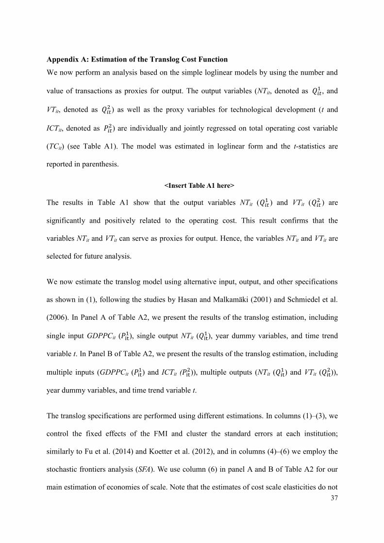
37

Appendix A: Estimation of the Translog Cost Function We now perform an analysis based on the simple loglinear models by using the number and

value of transactions as proxies for output. The output variables (NTit, denoted as 𝑄𝑖𝑡1 , and

VTit, denoted as 𝑄𝑖𝑡2 ) as well as the proxy variables for technological development (t and

ICTit, denoted as 𝑃𝑖𝑡2) are individually and jointly regressed on total operating cost variable

(TCit) (see Table A1). The model was estimated in loglinear form and the t-statistics are

reported in parenthesis.

<Insert Table A1 here>

The results in Table A1 show that the output variables NTit (𝑄𝑖𝑡1 ) and VTit (𝑄𝑖𝑡

2 ) are

significantly and positively related to the operating cost. This result confirms that the

variables NTit and VTit can serve as proxies for output. Hence, the variables NTit and VTit are

selected for future analysis.

We now estimate the translog model using alternative input, output, and other specifications

as shown in (1), following the studies by Hasan and Malkamäki (2001) and Schmiedel et al.

(2006). In Panel A of Table A2, we present the results of the translog estimation, including

single input GDPPCit (𝑃it1), single output NTit (𝑄it

1), year dummy variables, and time trend

variable t. In Panel B of Table A2, we present the results of the translog estimation, including

multiple inputs (GDPPCit (𝑃it1) and ICTit (𝑃it

2)), multiple outputs (NTit (𝑄it1) and VTit (𝑄it

2)),

year dummy variables, and time trend variable t.

The translog specifications are performed using different estimations. In columns (1)–(3), we

control the fixed effects of the FMI and cluster the standard errors at each institution;

similarly to Fu et al. (2014) and Koetter et al. (2012), and in columns (4)–(6) we employ the

stochastic frontiers analysis (SFA). We use column (6) in panel A and B of Table A2 for our

main estimation of economies of scale. Note that the estimates of cost scale elasticities do not

38

change substantially under different estimations; see the last line in Table A2.

The translog specifications in Table A2 have significant second-order terms confirming that

the use of translog form is appropriate. With technological development, the sign of the

coefficients of time trend variable t or year dummy variables should be negative, indicating

that the cost function is shifting downward over time. Based on this observation, stochastic

frontiers analysis (SFA) might be a preferred estimation method because the coefficients of

year dummy variables are negative and the significance level of the second-order terms is

higher compared to other model specifications.


For a robustness check, we also perform an analysis on the subsample for which the

institutions report the direct personnel cost in their financial statements; see Table A3. In

Panel A of Table A3, we report the results of the subsamples by using GDP per capita

(GDPPCit (𝑃it1)) as a measure of labor cost and number of transactions (NTit (𝑄it

1)) as output,

and, in Panel B of Table A3, we report the results of the subsample by using the personnel

cost (STAFFit (𝑃𝑖𝑡3)) as a measure of labor cost and the number of transactions (NTit (𝑄it

1)) as

output. We notice that the results of the subsample yield similar results by using GDP per

capita (𝑃𝑖𝑡1) and personnel expense (𝑃𝑖𝑡

3) as a different measure of labor cost; this provides

empirical support that GDP per capita (GDPPCit) is a reliable measure of labor cost for the

total sample.


39

Appendix B: Analysis Based on Two-inputs and Four-outputs Model

Now we expand our previous analysis and allow for four outputs to distinguish among

different businesses that stock exchanges, clearing houses, and CDSs perform.

We first use variables Number of transactions (NTit, denoted as 𝑄𝑖𝑡1

) and Value of

transactions (VTit, denoted as 𝑄𝑖𝑡2

) as two measures of the similar operations of FMIs.

Considering the different content and value of the services provided by stock exchanges,

CSDs, and clearing houses, we introduce the third output variable Number of listed

companies / Number of issuers (NLCSit, denoted as 𝑄𝑖𝑡3

) that equals to the number of listed

companies for stock exchanges and the number of issuers for CSDs and clearing houses. For

stock exchanges, the number of listed companies is used as a proxy for the stock exchange’s

effort to monitor how company-specific information is released and whether companies

observe the regulations set by the marketplace. For CSDs and clearing houses, the number of

issuers is used as proxy for number of issuers using the CSD notary service. The fourth

output variable Market capitalization / Securities held on accounts (MCSAit, denoted as 𝑄𝑖𝑡4

)

indicates the market capitalization of the stock exchanges and the value of securities held on

accounts for CSDs and clearing houses. For stock exchanges, the variable market

capitalization is defined as the total number of issued shares of companies multiplied by their

respective prices at a given time. For CSDs and clearing houses, the securities held on

accounts is defined as the Value of securities held on accounts.15,16,17

The definition of input variables is the same as before: variable GDP per capita (GDPPCit,

denoted as 𝑃𝑖𝑡1

) measures the labor cost for different countries at different years, and the ratio

of the country-specific share of information and communication technology expenditure to

15

For the selection of outputs variables, see also Malkamäki (1999), Hasan and Malkamäki (2001), Schmiedel (2001, 2002),

Schmiedel et al. (2006), and Serifsoy (2007). 16

The detail information for the variables of stock exchanges can be found on the webpage of World Federation of

Exchange (WFE). See https://www.world-exchanges.org/home/index.php/statistics/statistics-definitions. 17

The detail information for the variables of CSDs and clearing houses can be found on the webpage of European Central

Securities Depositories Association (ECSDA). See http://ecsda.eu/wp-content/uploads/ECSDA_DB_Methodology.pdf.

https://www.world-exchanges.org/home/index.php/statistics/statistics-definitions

http://ecsda.eu/wp-content/uploads/ECSDA_DB_Methodology.pdf

40

GDP (ICTit, denoted as 𝑃𝑖𝑡2

) measures the technology investments. The information of

number of issuers and securities held on accounts for CSDs and clearing houses is only

available from 2010 onwards. Therefore, we focus on the period between 2010 and 2015.18

<Insert Table B1 & Table B2 here>

Table B1 indicates that, based on the two-inputs and four-outputs model, economies of scale

are higher for large institutions than for smaller ones and if FMI providers are vertically or

horizontally integrated. FMI providers that offer services for a broad range of asset classes

have higher economies of scale compared to the FMI providers that offer services for a

narrow range of asset classes. Economies of scale are the highest for clearing houses, lower

for CSDs, and the lowest for stock exchanges.

Table B2 indicates that larger institutions have lower cost, revenue, scale, and allocative

efficiency, but higher profit efficiency. Horizontal integration is associated with lower cost,

allocative, and profit efficiency, but higher revenue and scale efficiency whereas vertical

integration is associated with higher revenue and scale efficiency. FMI providers that focus

on a broad range of asset classes operate less efficiently than FMI providers that focus on a

narrow range of asset classes. Clearing houses on average have higher scale efficiency and

profit efficiency, while stock exchanges on average have higher technical efficiency.

In sum, the results from two-inputs and four-outputs model are consistent with our conclusion

based on the two-inputs and two-outputs model.

18 For some outputs variables which equals to zero (because certain FMI providers do not engage in all businesses) or

missing, we follow the study of Beijnen and Bolt (2009) and set the missing outputs to a small value (0.0001).

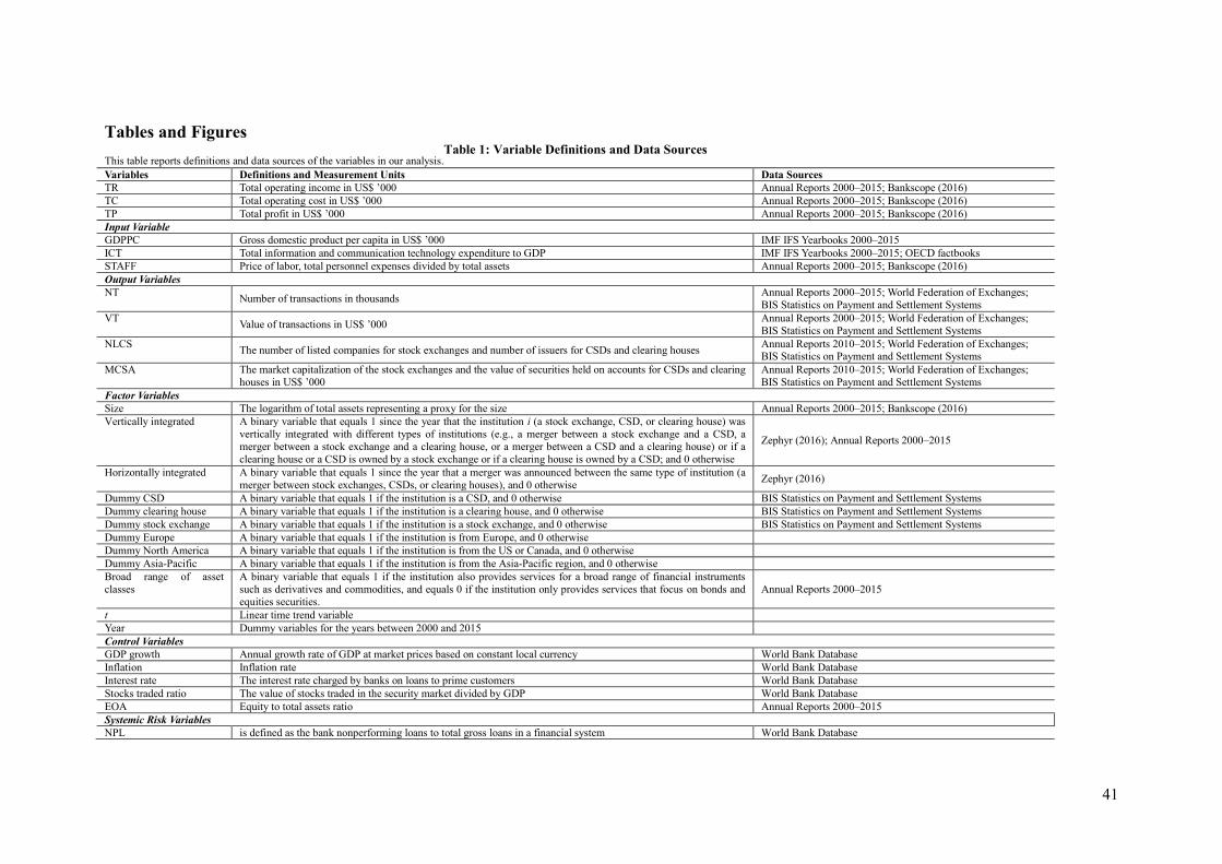
41

Tables and Figures Table 1: Variable Definitions and Data Sources

This table reports definitions and data sources of the variables in our analysis.

Variables Definitions and Measurement Units Data Sources

TR Total operating income in US$ ’000 Annual Reports 2000–2015; Bankscope (2016)

TC Total operating cost in US$ ’000 Annual Reports 2000–2015; Bankscope (2016)

TP Total profit in US$ ’000 Annual Reports 2000–2015; Bankscope (2016)

Input Variable

GDPPC Gross domestic product per capita in US$ ’000 IMF IFS Yearbooks 2000–2015

ICT Total information and communication technology expenditure to GDP IMF IFS Yearbooks 2000–2015; OECD factbooks

STAFF Price of labor, total personnel expenses divided by total assets Annual Reports 2000–2015; Bankscope (2016)

Output Variables

NT Number of transactions in thousands

Annual Reports 2000–2015; World Federation of Exchanges;

BIS Statistics on Payment and Settlement Systems

VT Value of transactions in US$ ’000



NLCS The number of listed companies for stock exchanges and number of issuers for CSDs and clearing houses

Annual Reports 2010–2015; World Federation of Exchanges; BIS Statistics on Payment and Settlement Systems

MCSA The market capitalization of the stock exchanges and the value of securities held on accounts for CSDs and clearing

houses in US$ ’000



Factor Variables

Size The logarithm of total assets representing a proxy for the size Annual Reports 2000–2015; Bankscope (2016)

Vertically integrated A binary variable that equals 1 since the year that the institution i (a stock exchange, CSD, or clearing house) was

vertically integrated with different types of institutions (e.g., a merger between a stock exchange and a CSD, a

merger between a stock exchange and a clearing house, or a merger between a CSD and a clearing house) or if a

clearing house or a CSD is owned by a stock exchange or if a clearing house is owned by a CSD; and 0 otherwise

Zephyr (2016); Annual Reports 2000–2015

Horizontally integrated A binary variable that equals 1 since the year that a merger was announced between the same type of institution (a

merger between stock exchanges, CSDs, or clearing houses), and 0 otherwise Zephyr (2016)

Dummy CSD A binary variable that equals 1 if the institution is a CSD, and 0 otherwise BIS Statistics on Payment and Settlement Systems

Dummy clearing house A binary variable that equals 1 if the institution is a clearing house, and 0 otherwise BIS Statistics on Payment and Settlement Systems

Dummy stock exchange A binary variable that equals 1 if the institution is a stock exchange, and 0 otherwise BIS Statistics on Payment and Settlement Systems

Dummy Europe A binary variable that equals 1 if the institution is from Europe, and 0 otherwise

Dummy North America A binary variable that equals 1 if the institution is from the US or Canada, and 0 otherwise

Dummy Asia-Pacific A binary variable that equals 1 if the institution is from the Asia-Pacific region, and 0 otherwise

Broad range of asset

classes

A binary variable that equals 1 if the institution also provides services for a broad range of financial instruments

such as derivatives and commodities, and equals 0 if the institution only provides services that focus on bonds and

equities securities.

Annual Reports 2000–2015

t Linear time trend variable

Year Dummy variables for the years between 2000 and 2015

Control Variables

GDP growth Annual growth rate of GDP at market prices based on constant local currency World Bank Database

Inflation Inflation rate World Bank Database

Interest rate The interest rate charged by banks on loans to prime customers World Bank Database

Stocks traded ratio The value of stocks traded in the security market divided by GDP World Bank Database

EOA Equity to total assets ratio Annual Reports 2000–2015

Systemic Risk Variables

NPL is defined as the bank nonperforming loans to total gross loans in a financial system World Bank Database

42

Table 1: Variable Definitions and Data Sources This table reports definitions and data sources of the variables in our analysis.

Variables Definitions and Measurement Units Data Sources

Stock Market Index

Volatility

The volatility of the stock market index return for each country at each year and calculated based on the monthly

return of the stock market index World Bank Database

CLIFS The country-level index of financial stress European Central Bank

Stock Market Efficiency Variables

Stock Market

Capitalization Ratio The market capitalization of listed domestic companies to GDP ratio World Bank Database

Banking System Asset to

GDP Ratio The banking system asset to GDP ratio. World Bank Database

43

Table 2: Data Statistics for Total Sample and Subsamples

This table reports summary statistics of the variables for the full sample, and different subsamples according to type, specialization, and horizontal and vertical integration of FMI. Our sample period is 2000–2015. All data are inflation-adjusted.

Total Sample

Different Types Specialization Horizontally Integrated Vertically Integrated

Stock

Exchanges

Clearing

Houses CSDs

Broad Range of

Asset Classes = 1

Broad Range of

Asset Classes = 0

Horizontally

Integrated = 1

Horizontally

Integrated = 0

Vertically

Integrated = 1

Vertically

Integrated = 0

Variable

Mean

(Standard

Deviation)

Min Max

Mean

(Standard

Deviation)

Mean

(Standard

Deviation)

Mean

(Standard

Deviation)

Mean

(Standard

Deviation)

Mean

(Standard

Deviation)

Mean

(Standard

Deviation)

Mean

(Standard

Deviation)

Mean

(Standard

Deviation)

Mean

(Standard

Deviation)

TC (US$ million) 256.85 0.05 6481 364.82 113.74 268.31 343.54 78.11 1397.57 154.38 449.15 200.87

(590.85) (864) (131.10) (375.20) (698) (129.86) (1312.3) (317.59) (754.42) (521.67)

TR (US$ million) 348.90 0.1 6861 525.74 198.58 330.08 471.9 95.24 1858.8 213.27 602.96 274.93

(735) (1072.50) (191.50) (432) (863.8) (146.1) (1540.4) (394.76) (1016.46) (611.73)

GDPPC (US$ ’000) 32.21 0.46 116.6 21.55 35.60 42.48 32.5 31.56 42.65 31.33 39.96 29.92

(23.01) (15.80) (17.10) (29.86) (25.7) (23.7) (10.1) (23.57) (23.93) (22.25)

ICT (%) 1.66 0.08 3.47 1.33 1.97 1.71

1.73 1.51 2.2 1.60 2.03 1.54

(0.80) (0.88) (0.64) (0.76) (0.81) (0.78) (0.52) (0.81) (0.84) (0.76)

Personnel expense (US$ million) 78.81 0.07 949 85.84 44.27 107.45 102 32 293.9 58.60 100.53 72.38

(140) (166) (51.02) (156.80) (161.3) (59.20) (282.5) (96.56) (154.41) (134.99)

NT (million) 1305.89 0.02 23254 803.57 2128.74 1079.54 1005.5 1925.22 1107.5 1323.71 2278.12 1022.81

(3125) (1353) (4259) (3203) (2535.1) (4018) (1133.6) (3244.75) (4553.49) (2500.56)

VT (US$ billion) 66620 0.08 23252000 4477 403300 63980 37840 139200 25230 72410 205100 15790

(233900) (30060) (552700) (110600) (90800) (407000) (69660) (247900) (415400) (47520)

EOA (%) 31.51 0.05 99.4 52.58 7.93 27.37 32.39 29.61 36.37 31.08 24.69 33.60

(31.66) (29.24) (21.20) (29.10) (31.85) (31.24) (25.8) (32.12) (32.00) (31.30)

Total assets (US$ billion) 1104 0 679900 65.33 3367 6.56 1640 3.53 184.4 1184 130.15 1418

(26850) (616.80) (47480) (8.70) (32750) (6.83) (981) (27990) (89.10) (30530)

Size 13.81 4.4 27.25 12.75 14.57 14.40 14.44 12.53 13.68 15.38 13.49 14.9

(2.89) (3) (2.92) (2.23) (2.67) (2.9) (2.8) (3.47) (2.88) (2.68)

Vertically integrated 0.23 0 1 0.15 0.26 0.30 0.23 0.005 0.434 0.21 1 0

(0.42) (0.36) (0.44) (0.46) (0.42) (0.069) (0.50) (0.41) (0) (0)

Horizontally integrated 0.08 0 1 0.18 0 0.04 0.11 0.03 1 0 0.159 0.06

(0.28) (0.39) (0) (0.19) (0.31) (0.17) (0) (0) (0.37) (0.24)

GDP growth (%) 2.35 −9.13 27.5 2.97 1.93 1.99 2.45 2.14 1.68 2.41 1.92 2.48

(3.30) (3.73) (2.82) (3.10) (3.43) (3.01) (2.95) (3.32) (2.97) (3.38)

Inflation 3.40 −6 103.8 4.33 3.03 2.57 2.94 4.36 1.60 3.56 2.63 3.63

(5.72) (7.94) (4.20) (2.69) (3.57) (8.55) (0.97) (5.94) (3.2) (6.26)

Interest rate 2.92 −42.3 44.6 3.63 1.93 3.14 3.10 2.52 2.40 2.97 3.63 2.73

(5.18) (6.60) (3.40) (3.27) (4.71) (6.18) (2.33) (5.38) (6.8) (4.66)

Stock traded ratio (%) 80.58 0.02 952.7 77.83 106.71 55.03 92.19 55.90 116.8 77.28) 93.97 76.59

(102.29) (127.70) (92.80) (60.20) (111.6) (73.2) (89.6) (102.81 (94.61) (104.24)

44

Table 3: Average Key Performance Ratios This table presents the mean of performance ratios for the total sample, and various subsamples according to institution size, horizontal and vertical integration, type, specialization, and geographical location. Our sample period is

2000–2015. All currency and price-related data are inflation-adjusted and expressed in US$. TC is operating cost in US$ ’000; TR is operating income in US$ ’000; NT is the number of transactions in thousands; VT is the value of

transactions in US$ ’000. TC/NT indicates cost per trade; TC/VT indicates cost per value of transactions; TR/NT indicates operating income per trade; TR/VT indicates operating income per value of transactions; VT/NT indicates

value per transactions. Significance of group mean differences: * Significant at the 10% level. ** Significant at the 5% level. *** Significant at the 1% level.

Sample N TC/NT TC/VT TR/NT TR/VT VT/NT (US$ million)

All 403 158.20 0.002263 272.96 0.002281 146.59

Institution Size Quantile 4 (Largest) 99 917.16 0.000263 1584.49 0.000342 604.59 Quantile 3 98 47.83 0.000688 148.14 0.000986 0.96 Quantile 2 98 1.61 0.001040 3.63 0.002456 0.39 Quantile 1 (Smallest) 98 12.58 0.005514 14.51 0.005680 0.04

Top 50% 196 308.40 0.000402 543.21 0.000572 333.57 Bottom 50% 197 10.81 0.003164 13.38 0.003766 0.34

Group Mean Difference 297.59*** −0.00276*** 529.83*** −0.00319*** 333.23***

Type of Integration

Horizontally integrated 57 45.51 0.003171 39.90 0.000722 3.50

Non-horizontally integrated 346 170.02 0.002113 297.41 0.002539 170.30

Group Mean Difference −124.51*** 0.001058 −257.51*** −0.00182*** −166.8***

Vertically integrated 105 498.75 0.000262 740.39 0.000333 553.67

Non-vertically integrated 298 61.00 0.002973 139.54 0.002972 2.19


Specialization Broad range of asset classes 292 225.11 0.001426 391.36 0.001534 201.24

Narrow range of asset classes 111 17.06 0.004451 23.18 0.004233 3.81


Regions Europe 219 200.51 0.002046 284.17 0.002732 7.89 North America 47 1.56 0.000066 1.71 0.000076 267.16 Asia-Pacific 109 122.13 0.001423 430.04 0.002653 1.56 South America & Africa 28 1.66 0.005544 2.33 0.006369 0.050

Type of FMI CSDs

100 423.77 0.000700 616.38 0.000773 580.08

Group Mean Difference between Different Subsamples Top 50% − Bottom 50% 781.4*** −0.00052 1164.1*** −0.000051 1347.2***

Broad range of asset classes − Narrow range of asset classes 629.42*** 0.00081** 934.17*** 0.0009** 772.68***

Horizontally integrated − Non-horizontally integrated −221.92 −0.0007** −341.17 −0.00078** −491.01**

Vertically integrated − Non-vertically integrated 1159.93*** −0.00098** 1762.6*** −0.00105** 1515.9***

Stock Exchanges 257 63.16 0.003281 202.95 0.003283 0.51 Group Mean Difference between Different Subsamples

Top 50% − Bottom 50% 118.2*** −0.00399*** 416.34*** −0.00453*** 1.08***

Broad range of asset classes − Narrow range of asset classes 77.1*** −0.00672*** 255.03*** −0.00616*** 0.65***

Horizontally integrated − Non-horizontally integrated −48.86* 0.000004 −246.34*** −0.00323*** −0.61***

Vertically integrated − Non-vertically integrated −71.98*** −0.0031*** −234.24*** −0.00289*** −0.57***

Clearing Houses 46 38.71 0.000009 50.84 0.000012 14.00

Group Mean Difference between Different Subsamples Top 50% − Bottom 50%

76.79** 0.000009 90.66** 0.00 11.59***

Broad range of asset classes − Narrow range of asset classes 60.7** 0.00002 69.06** 0.000019 −1.46

Vertically integrated − Non-vertically integrated 50.34 0.000002 61.51 0.00 −4.11

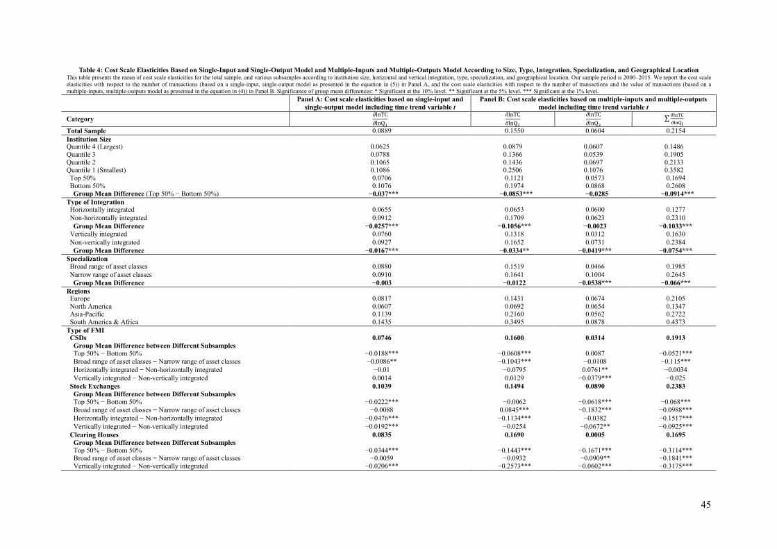
45

Table 4: Cost Scale Elasticities Based on Single-Input and Single-Output Model and Multiple-Inputs and Multiple-Outputs Model According to Size, Type, Integration, Specialization, and Geographical Location This table presents the mean of cost scale elasticities for the total sample, and various subsamples according to institution size, horizontal and vertical integration, type, specialization, and geographical location. Our sample period is 2000–2015. We report the cost scale

elasticities with respect to the number of transactions (based on a single-input, single-output model as presented in the equation in (5)) in Panel A, and the cost scale elasticities with respect to the number of transactions and the value of transactions (based on a

multiple-inputs, multiple-outputs model as presented in the equation in (4)) in Panel B. Significance of group mean differences: * Significant at the 10% level. ** Significant at the 5% level. *** Significant at the 1% level.

Panel A: Cost scale elasticities based on single-input and

single-output model including time trend variable t

Panel B: Cost scale elasticities based on multiple-inputs and multiple-outputs

model including time trend variable t

Category ∂lnTC

𝜕lnQ1

∂lnTC

∂lnQ1

∂lnTC

∂lnQ2

∑∂lnTC

∂lnQi

Total Sample 0.0889 0.1550 0.0604 0.2154

Institution Size Quantile 4 (Largest) 0.0625 0.0879 0.0607 0.1486 Quantile 3 0.0788 0.1366 0.0539 0.1905 Quantile 2 0.1065 0.1436 0.0697 0.2133 Quantile 1 (Smallest) 0.1086 0.2506 0.1076 0.3582 Top 50% 0.0706 0.1121 0.0573 0.1694 Bottom 50% 0.1076 0.1974 0.0868 0.2608 Group Mean Difference (Top 50% − Bottom 50%) −0.037*** −0.0853*** −0.0285 −0.0914***

Type of Integration Horizontally integrated 0.0655 0.0653 0.0600 0.1277

Non-horizontally integrated 0.0912 0.1709 0.0623 0.2310

Group Mean Difference −0.0257*** −0.1056*** −0.0023 −0.1033***

Vertically integrated 0.0760 0.1318 0.0312 0.1630

Non-vertically integrated 0.0927 0.1652 0.0731 0.2384

Group Mean Difference −0.0167*** −0.0334** −0.0419*** −0.0754***

Specialization Broad range of asset classes 0.0880 0.1519 0.0466 0.1985

Narrow range of asset classes 0.0910 0.1641 0.1004 0.2645

Group Mean Difference −0.003 −0.0122 −0.0538*** −0.066***

Regions Europe 0.0817 0.1431 0.0674 0.2105 North America 0.0607 0.0692 0.0654 0.1347 Asia-Pacific 0.1139 0.2160 0.0562 0.2722 South America & Africa 0.1435 0.3495 0.0878 0.4373

Type of FMI CSDs 0.0746 0.1600 0.0314 0.1913

Group Mean Difference between Different Subsamples Top 50% − Bottom 50% −0.0188*** −0.0608*** 0.0087 −0.0521***

Broad range of asset classes − Narrow range of asset classes −0.0086** −0.1043*** −0.0108 −0.115***

Horizontally integrated − Non-horizontally integrated −0.01 −0.0795 0.0761** −0.0034

Vertically integrated − Non-vertically integrated 0.0014 0.0129 −0.0379*** −0.025

Stock Exchanges 0.1039 0.1494 0.0890 0.2383

Group Mean Difference between Different Subsamples Top 50% − Bottom 50% −0.0222*** −0.0062 −0.0618*** −0.068***

Broad range of asset classes − Narrow range of asset classes −0.0088 0.0845*** −0.1832*** −0.0988***

Horizontally integrated − Non-horizontally integrated −0.0476*** −0.1134*** −0.0382 −0.1517***

Vertically integrated − Non-vertically integrated −0.0192*** −0.0254 −0.0672** −0.0925***

Clearing Houses 0.0835 0.1690 0.0005 0.1695

Group Mean Difference between Different Subsamples Top 50% − Bottom 50% −0.0344*** −0.1443*** −0.1671*** −0.3114*** Broad range of asset classes − Narrow range of asset classes −0.0059 −0.0932 −0.0909** −0.1841*** Vertically integrated − Non-vertically integrated −0.0206*** −0.2573*** −0.0602*** −0.3175***

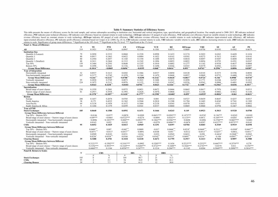
46

Table 5: Summary Statistics of Efficiency Scores

This table presents the means of efficiency scores for the total sample, and various subsamples according to institution size, horizontal and vertical integration, type, specialization, and geographical location. Our sample period is 2000–2015. TE indicates technical

efficiency, PTE indicates pure technical efficiency, CE indicates cost efficiency based on constant returns to scale technology, CEScope indicates CE purged of scale efficiency, VCE indicates cost efficiency based on variable returns to scale technology, RE indicates

revenue efficiency based on constant returns to scale technology, REScope indicates RE purged of scale efficiency, VRE indicates revenue efficiency based on variable returns to scale technology, SE indicates input-oriented scale efficiency, AE indicates

input-oriented allocative efficiency, PE indicates profit efficiency estimated based on Cooper et al. (2004, Eq. (8.1)), CRS indicates constant returns to scale, VRS indicates variable returns to scale, IRS indicates increasing returns to scale, DRS indicates decreasing

returns to scale. Significance of group mean differences: * Significant at the 10% level. ** Significant at the 5% level. *** Significant at the 1% level.

Panel A: Mean of Efficiency

N TE PTE CE CEScope VCE RE REScope VRE SE AE PE

All 319 0.1921 0.2568 0.0947 0.1318 0.1301 0.0571 0.0809 0.0756 0.8193 0.4562 0.0679

Institution Size Quantile 4 (Largest) 79 0.2058 0.3333 0.0860 0.1528 0.0998 0.1633 0.2174 0.2022 0.6263 0.4420 0.1634 Quantile 3 80 0.0917 0.1863 0.0422 0.0984 0.1022 0.0142 0.0392 0.0273 0.7613 0.4851 0.0143 Quantile 2 80 0.2584 0.2857 0.1160 0.1358 0.1488 0.0474 0.0634 0.0697 0.9287 0.4688 0.0645 Quantile 1 (Smallest) 80 0.2411 0.2464 0.1515 0.1542 0.1896 0.0055 0.0055 0.0056 0.9793 0.4391 0.0347 Top 50% 159 0.1484 0.2593 0.0640 0.1255 0.1010 0.0882 0.1277 0.1142 0.9538 0.4637 0.0884 Bottom 50% 160 0.2498 0.2662 0.1336 0.1450 0.1690 0.0266 0.0347 0.0379 0.6942 0.4541 0.0497

Group Mean Difference −0.1014***

−0.0069 −0.0696***

−0.0195 −0.068***

0.0616***

0.093***

0.0763***

0.2596***

0.0096 0.0387*

Type of Integration Horizontally integrated 52 0.0537 0.1613 0.0282 0.1066 0.0337 0.0050 0.0120 0.0145 0.5273 0.5396 0.0050 Non-horizontally integrated 267 0.2177 0.2745 0.1070 0.1364 0.1479 0.0668 0.0937 0.0869 0.8733 0.4408 0.0795


−0.1132***

−0.0788***

−0.0298 −0.1142***

−0.0618**

−0.0817**

−0.0724**

−0.346***

0.0988**

−0.0745**

Vertically integrated 95 0.2038 0.3749 0.0873 0.1823 0.1606 0.1411 0.2058 0.1771 0.6344 0.4747 0.1412 Non-vertically integrated 224 0.1875 0.2111 0.0976 0.1122 0.1183 0.0247 0.0326 0.0363 0.8908 0.4491 0.0395

Group Mean Difference 0.0163 0.1638***

−0.0103 0.0701***

0.0423 0.1164***

0.1732***

0.1408***

−0.2564***

0.0256 0.1017***

Specialization Broad range of asset classes 238 0.1559 0.2081 0.0575 0.0851 0.0672 0.0466 0.0665 0.0617 0.7976 0.4402 0.0513 Narrow range of asset classes 81 0.2937 0.3938 0.1993 0.2628 0.3070 0.0868 0.1215 0.1146 0.8802 0.5012 0.1144


−0.1857***

−0.1418***

−0.1777***

−0.2398***

−0.0402* −0.055

** −0.0529

* −0.0826

** −0.061 −0.0631

**

Region Europe 208 0.1657 0.2078 0.0705 0.0910 0.084 0.0514 0.0727 0.0659 0.8647 0.4257 0.0517 North America 38 0.175 0.4225 0.1362 0.2944 0.2818 0.1308 0.1784 0.1603 0.4242 0.7341 0.1309 Asia-Pacific 64 0.3138 0.3458 0.1672 0.1884 0.2138 0.0365 0.0570 0.0651 0.911 0.4143 0.0952 South America & Africa 9 0.1204 0.1379 0.0299 0.0341 0.0337 0.0060 0.0069 0.0060 0.8794 0.2467 0.0066

Type of FMI Stock Exchanges 185 0.0640 0.1580 0.0592 0.1471 0.1666 0.0243 0.149 0.0923 0.3013 0.9320 0.0700 Group Mean Difference between Different

Subsamples

Top 50% − Bottom 50% −0.0146 −0.057* −0.0078 −0.0509 −0.0651*** 0.0205*** 0.1473*** −0.0742 0.136*** −0.0243 −0.0105 Broad range of asset classes − Narrow range of asset classes −0.09*** −0.0465 −0.0722*** −0.0274 −0.0095 0.0163** 0.1135** 0.0871 −0.1697*** 0.0203 0.0084** Horizontally integrated − Non-horizontally integrated −0.0096 −0.1053*** −0.004*** −0.0923*** −0.1062*** 0.0386*** −0.0698 −0.0496 −0.2784*** −0.0607*** −0.0401 Vertically integrated − Non-vertically integrated

0.0143 0.052 0.0192 0.041 −0.0378 0.0496*** −0.0474 0.0297 0.4157*** 0.0575*** 0.0143 CSDs 95 0.0452 0.1029 0.0413 0.0969 0.1291 0.0397 0.0784 0.0403 0.3549 0.9519 0.0398 Group Mean Difference between Different

Subsamples

Top 50% − Bottom 50% 0.0489

*** 0.007 −0.042

*** 0.0009 −0.017 0.0446

*** 0.0218

* 0.0449

*** 0.2311

*** −0.0309

* 0.0447

***

Broad range of asset classes − Narrow range of asset classes −0.0571***

−0.0117 −0.0517***

−0.0091 0.0108 −0.051***

−0.0112 −0.0513***

−0.4257***

−0.0011 −0.0511***

Horizontally integrated − Non-horizontally integrated 0.0509 0.0183 0.0231 −0.016 −0.033 0.0565 0.0433 0.058 −0.4414

* −0.2848

*** 0.0565

Vertically integrated − Non-vertically integrated

0.0236* 0.0354

*** 0.0166 0.0255

** 0.0342

** 0.0315

** 0.0495

*** 0.0316

*** −0.106 0.0507

*** 0.0314

***

Clearing Houses 39 0.3488 0.4701 0.3418 0.4228 0.4672 0.1795 0.2917 0.2413 0.7422 0.9097 0.2980 Group Mean Difference between Different

Subsamples

Top 50% − Bottom 50% 0.3121*** −0.3502*** −0.3181*** −0.0902 −0.3205*** 0.1436 0.5215*** 0.2532** 0.6447*** −0.2574*** 0.278 Broad range of asset classes − Narrow range of asset classes −0.3192*** −0.4935*** −0.3169*** −0.4204*** −0.4723*** −0.1608** −0.3426*** −0.2743*** −0.0378 0.011 −0.356*** Vertically integrated − Non-vertically integrated

0.4468*** 0.1184 0.4558*** 0.247*** 0.1214 0.204*** −0.1142 0.0204 0.5849*** 0.2098*** 0.3816***

Panel B: Return to Scales N CRS IRS DRS

N % N % N % Stock Exchanges 185 0 0 164 88.7 21 11.3 CSDs 95 2 2.1 54 56.8 39 41.1 Clearing Houses 39 3 7.7 24 61.5 12 30.8

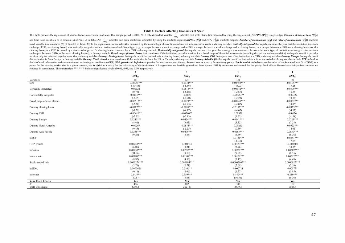
47

Table 6: Factors Affecting Economies of Scale

This table presents the regressions of various factors on economies of scale. Our sample period is 2000–2015. The dependent variable 𝟏

𝑬𝑺𝟏𝒊𝒕 indicates cost scale elasticities estimated by using the single-input (GDPPCit (𝑷𝒊𝒕

𝟏 )), single-output (Number of transactions (𝑸𝒊𝒕𝟏 ))

and time trend variable t as in column (6) of Panel A in Table A2; 𝟏

𝑬𝑺𝟐𝒊𝒕 indicates cost scale elasticities estimated by using the multiple-inputs (GDPPCit (𝑷𝒊𝒕

𝟏 ) and ICTit (𝑷𝒊𝒕𝟐 )), multiple-outputs (Number of transactions (𝑸𝒊𝒕

𝟏 ) and Value of transactions (𝑸𝒊𝒕𝟐 )) and time

trend variable t as in column (6) of Panel B in Table A2. In the regressions, we include: Size measured by the natural logarithm of financial market infrastructures assets, a dummy variable Vertically integrated that equals one since the year that the institution i (a stock

exchange, CSD, or clearing house) was vertically integrated with an institution of a different type (e.g., a merger between a stock exchange and a CSD, a merger between a stock exchange and a clearing house, or a merger between a CSD and a clearing house) or if a

clearing house or a CSD is owned by a stock exchange or if a clearing house is owned by a CSD, a dummy variable Horizontally integrated that equals one since the year that a merger was announced between the same type of institutions (a merger between stock

exchanges, between CSDs, or between clearing houses), a dummy variable Broad range of asset classes that equals one if the institution provides services for a broad range of financial instruments (including derivatives and commodities) and equals zero if it provides

services only for debt and equities securities, a dummy variable Dummy clearing house that equals one if the institution is a clearing house, a dummy variable Dummy CSD that equals one if the institution is a CSD, a dummy variable Dummy Europe that equals one if

the institution is from Europe, a dummy variable Dummy North America that equals one if the institution is from the US or Canada, a dummy variable Dummy Asia-Pacific that equals one if the institution is from the Asia-Pacific region, the variable ICT defined as

the % of total information and communication technology expenditure to GDP, GDP growth and Inflation as proxies for macroeconomics factors, Interest rate as a proxy for monetary policy, Stocks traded ratio (based on the value of stocks traded in as % of GDP) as a

proxy for the security market size in a given country, and ln EOA as a proxy for the risk-taking of the institutions. All regressions are feasible generalized least square (FGLS) estimation and control for the yearly fixed effects. Heteroskedasticity-robust t-values are

reported in parentheses. The superscripts ***, **, * indicate significance levels of 0.01, 0.05, and 0.10, respectively.

𝟏

𝑬𝑺𝟏𝒊𝒕

𝟏

𝑬𝑺𝟐𝒊𝒕

𝟏

𝑬𝑺𝟏𝒊𝒕

𝟏

𝑬𝑺𝟐𝒊𝒕

Variables (1) (2) (3) (4)

Size -0.00551*** -0.0134*** -0.00450*** -0.0105*** (-15.88) (-6.16) (-13.03) (-5.25)

Vertically integrated 0.00122 -0.0613*** -0.00372*** -0.0599***

(0.78) (-6.18) (-2.67) (-6.38)

Horizontally integrated -0.0113*** -0.0125 -0.00563** -0.00322

(-3.85) (-1.20) (-2.29) (-0.36)

Broad range of asset classes -0.00512** -0.0423*** -0.00948*** -0.0302***

(-2.20) (-4.45) (-4.02) (-3.03)

Dummy clearing house -0.0187*** -0.0988*** -0.0107*** -0.0925***

(-7.59) (-4.17) (-4.67) (-4.12)

Dummy CSD -0.00611** -0.0240** 0.00378 -0.0176

(-2.35) (-2.13) (1.53) (-1.54)

Dummy Europe 0.0240*** 0.0424*** 0.0141*** 0.0723***

(8.41) (3.43) (3.32) (7.28)

Dummy North America 0.00267 -0.0874*** 0.00215 -0.0523***

(0.85) (-5.35) (0.50) (-4.05)

Dummy Asia-Pacific 0.0256*** 0.0499*** 0.0163*** 0.0630***

(9.23) (3.48) (3.39) (6.36)

ln ICT

-0.0121*** -0.0341***

(-6.38) (-7.84)

GDP growth 0.00252*** 0.000335 0.00153*** -0.000401

(6.06) (0.21) (3.26) (-0.35)

Inflation 0.00233*** 0.00916*** 0.00251*** 0.00687***

(11.96) (8.10) (9.82) (6.35)

Interest rate 0.00188*** 0.00584*** 0.00151*** 0.00512***

(8.92) (4.56) (7.17) (4.49)

Stocks traded ratio 0.0000274*** 0.000104*** 0.0000286*** 0.0000825***

(2.76) (2.71) (2.68) (2.59)

ln EOA 0.0000626 0.0106** 0.000718 0.00877*

(0.11) (2.06) (1.52) (1.85)

Intercept 0.143*** 0.359*** 0.147*** 0.289***

(17.67) (6.65) (16.56) (5.36)

Year Fixed Effects Yes Yes Yes Yes

N 486 182 383 182 Wald Chi-square 8274.1 2621.8 2839.3 9086.8

48

Table 7: Factors Affecting Efficiency

This table presents the regressions of various factors on efficiency. Our sample period is 2000–2015. The dependent variable TE indicates technical efficiency, PTE indicates pure technical efficiency, CE indicates cost efficiency based on constant returns to scale

technology, CEScope indicates CE purged of scale efficiency, VCE indicates cost efficiency based on variable returns to scale technology, RE indicates revenue efficiency based on constant returns to scale technology, REScope indicates RE purged of scale

efficiency, VRE indicates revenue efficiency based on variable returns to scale technology, SE indicates input-oriented scale efficiency, AE indicates input-oriented allocative efficiency, and PE indicates profit efficiency estimated based on Cooper et al. (2004, Eq.

(8.1)). In the regressions, we include: Size measured by the natural logarithm of FMI assets, a dummy variable Vertically integrated that equals one since the year that the FMI provider i was vertically integrated with a FMI provider of a different type (e.g., a merger

between a stock exchange and a CSD, a merger between a stock exchange and a clearing house, or a merger between a CSD and a clearing house) or if a clearing house or a CSD is owned by a stock exchange or if a clearing house is owned by a CSD, a dummy

variable Horizontally integrated that equals one since the year of a merger between the same type of institutions (a merger between stock exchanges, CSDs, or clearing houses), a dummy variable Broad range of asset classes that equals one if the institution provides

services for a broad range of financial instruments (including derivatives and commodities) and equals zero if it provides services only for debt and equities securities, a dummy variable Dummy clearing house that equals one if the institution is a clearing house,

dummy variable Dummy CSD that equals one if the institution is a CSD, a dummy variable Dummy Europe that equals one if the institution is from Europe, a dummy variable Dummy North America that equals one if the institution is from the US or Canada, a

dummy variable Dummy Asia-Pacific that equals one if the institution is from the Asia-Pacific region, GDP growth and Inflation as proxies for macroeconomics factors, Interest rate as a proxy for monetary policy, Stocks traded ratio (based on the value of stocks

traded as % of GDP) as a proxy for the security market size in a given country, and ln EOA as a proxy for the risk-taking of the institutions. All regressions are feasible generalized least square (FGLS) estimation and control for the yearly fixed effects.

Heteroskedasticity-robust t-values are reported in parentheses. The superscripts ***, **, * indicate significance levels of 0.01, 0.05, and 0.10, respectively.

(1) (2) (3) (4) (5) (6) (7) (8) (9) (10) (11)

Variables TE PTE CE CEScope VCE RE REScope VRE SE AE PE

Size -0.00462 0.00384 -0.0103*** -0.00678* -0.0186*** 0.00259 0.0107* 0.00822 -0.0403*** -0.0428*** 0.00124

(-1.14) (0.70) (-3.23) (-1.69) (-4.21) (0.78) (1.70) (1.35) (-5.29) (-4.76) (0.33)

Vertically integrated 0.00442 0.0929*** 0.0210** 0.0573*** 0.0518** -0.00410 0.00852 -0.00643 -0.0568* 0.0190 0.00211

(0.24) (3.15) (2.00) (3.88) (2.49) (-0.22) (0.31) (-0.23) (-1.89) (0.66) (0.12)

Horizontally integrated -0.0211 -0.0980*** -0.0393** -0.0496** -0.0545** 0.0135 -0.0167 0.00115 -0.0157 -0.0474 0.00636

(-1.20) (-3.12) (-2.53) (-2.36) (-2.18) (0.86) (-0.82) (0.05) (-0.42) (-1.21) (0.38)

Broad range of asset classes -0.116*** -0.128*** -0.0770*** -0.132*** -0.0932*** -0.0107 -0.0221 0.000480 0.0187 0.0662 -0.0162

(-5.88) (-4.37) (-4.54) (-7.22) (-3.92) (-0.61) (-0.84) (0.02) (0.58) (1.58) (-0.82)

Dummy clearing house 0.119*** 0.598*** 0.0700** 0.184*** 0.272*** 0.180*** 0.263*** 0.245*** -0.196*** 0.0796 0.191***

(2.85) (8.89) (2.56) (4.46) (4.50) (4.02) (4.14) (3.62) (-2.99) (0.97) (3.82)

Dummy CSD 0.00786 0.0231 -0.0253 -0.0629*** -0.0221 0.0291 0.0486 0.0786** 0.0765** -0.0967** 0.0262

(0.41) (0.70) (-1.58) (-2.69) (-0.76) (1.39) (1.51) (2.47) (2.23) (-2.41) (1.07)

Dummy Europe -0.207*** -0.519*** -0.0524 -0.122*** -0.0840* -0.00935 -0.0863* -0.106* 0.199*** 0.0662 -0.0889

(-3.75) (-7.99) (-1.36) (-2.77) (-1.91) (-0.42) (-1.71) (-1.90) (5.04) (1.14) (-1.56)

Dummy North America -0.197*** -0.339*** 0.0155 0.0577 0.0479 -0.0250 -0.0844 -0.105* -0.331*** 0.683*** -0.0867

(-3.53) (-4.61) (0.38) (1.19) (0.98) (-0.83) (-1.44) (-1.70) (-7.09) (10.24) (-1.47)

Dummy Asia-Pacific -0.118** -0.325*** -0.0150 -0.0726 -0.0218 0.00683 0.0196 0.0209 0.0505 0.0370 -0.0593

(-2.12) (-4.84) (-0.39) (-1.63) (-0.54) (0.29) (0.39) (0.38) (1.33) (0.63) (-1.06)

GDP growth -0.000317 -0.0141** 0.000380 -0.00229 -0.00141 -0.000226 -0.00776** -0.00899** 0.0158*** 0.00250 0.000243

(-0.09) (-2.39) (0.15) (-0.77) (-0.38) (-0.11) (-2.02) (-2.38) (3.16) (0.36) (0.07)

Inflation 0.000598 -0.0130*** -0.000800 -0.00133 -0.000575 -0.000617 -0.00659** -0.00686** 0.00974*** 0.00794* -0.00154

(0.25) (-3.64) (-0.48) (-0.60) (-0.28) (-0.42) (-2.45) (-2.37) (2.90) (1.75) (-0.65)

Interest rate -0.00504*** -0.0143*** -0.00259** -0.00447*** -0.00341** -0.000352 -0.00241 -0.00367* 0.00802*** -0.00184 -0.00169

(-3.15) (-7.20) (-1.98) (-3.63) (-2.31) (-0.28) (-1.47) (-1.80) (3.42) (-0.89) (-0.89)

Stocks traded ratio -0.0000621 -0.0000897 -0.000101*** -0.0000567 -0.0000237 -0.0000215 -0.000159** -0.000198*** 0.000252** -0.000365*** -0.0000213

(-1.44) (-1.20) (-2.97) (-1.46) (-0.51) (-0.56) (-2.24) (-2.84) (2.13) (-4.10) (-0.46)

ln EOA 0.0105 0.0893*** 0.000452 0.0203** 0.0227** -0.00380 0.0118 0.00869 -0.0906*** -0.00806 -0.00132

(0.97) (6.02) (0.07) (2.39) (2.05) (-0.43) (0.82) (0.60) (-6.01) (-0.49) (-0.13)

Intercept 0.470*** 0.503*** 0.331*** 0.334*** 0.384*** -0.00959 -0.0913 -0.0511 1.632*** 0.692*** 0.0747

(3.44) (2.80) (4.30) (3.45) (3.79) (-0.13) (-0.60) (-0.32) (8.55) (3.35) (0.70)

Year Fixed Effects Yes Yes Yes Yes Yes Yes Yes Yes Yes Yes Yes

N 200 200 200 195 200 200 195 200 195 195 200

Wald Chi-square 181.8 426.0 151.8 663.0 231.5 42.58 100.6 95.98 1191.3 800.8 38.83

49

Table 8: Impact of Integration on the Efficiency of FMI Providers This table presents the regressions of the impact of financial integration on the efficiency of FMI providers. Our sample period is 2000–2015. The dependent variable TE indicates technical efficiency, PTE indicates pure technical efficiency, CE indicates cost

efficiency based on constant returns to scale technology, CEScope indicates CE purged of scale efficiency, VCE indicates cost efficiency based on variable returns to scale technology, RE indicates revenue efficiency based on constant returns to scale technology,

REScope indicates RE purged of scale efficiency, VRE indicates revenue efficiency based on variable returns to scale technology, SE indicates input-oriented scale efficiency, AE indicates input-oriented allocative efficiency, and PE indicates profit efficiency

estimated based on Cooper et al. (2004, Eq. (8.1)). Dummy variable Vertically integrated equals one since the year that the FMI provider i was vertically integrated with a FMI provider of a different type (e.g., a merger between a stock exchange and a CSD, a merger

between a stock exchange and a clearing house, or a merger between a CSD and a clearing house) or if a clearing house or a CSD is owned by a stock exchange or if a clearing house is owned by a CSD, dummy variable Horizontally integrated equals one since the

year of a merger between the same type of institutions (a merger between stock exchanges, CSDs, or clearing houses), dummy variable Broad range of asset classes equals one if the institution provides services for a broad range of financial instruments (including

derivatives and commodities) and equals zero if it provides services only for debt and equities securities, a dummy variable Dummy clearing house equals one if the institution is a clearing house, a dummy variable Dummy CSD equals one if the institution is a CSD,

and a dummy variable Dummy stock exchange equals one if the institution is a stock exchange. All regressions are feasible generalized least square (FGLS) estimation and control for the yearly fixed effects. Heteroskedasticity-robust t-values are reported in

parentheses. The superscripts ***, **, * indicate significance levels of 0.01, 0.05, and 0.10, respectively.

Panel A (1) (2) (3) (4) (5) (6) (7) (8) (9) (10) (11) Variables TE PTE CE CEScope VCE RE REScope VRE SE AE PE

Horizontally integrated * Dummy stock exchange -0.0656*** -0.131*** -0.0653*** -0.0699*** -0.0743*** 0.00251 -0.0269 -0.0148 0.0340 -0.0686 0.000308

(-2.70) (-3.97) (-3.62) (-3.22) (-2.85) (0.14) (-1.29) (-0.63) (1.03) (-1.42) (0.02)

Horizontally integrated * Dummy CSD 0.0493 0.141*** 0.0572** 0.140*** 0.108*** 0.0827** 0.181*** 0.158*** -0.578*** 0.0112 0.0767

(1.56) (3.08) (2.51) (5.00) (2.72) (2.54) (3.59) (2.96) (-13.05) (0.19) (1.32)

Vertically integrated 0.0194 0.0961*** 0.0205* 0.0571*** 0.0520** -0.000614 0.00992 -0.00245 -0.0615** 0.0242 0.00553

(1.00) (3.26) (1.96) (3.97) (2.50) (-0.03) (0.37) (-0.09) (-2.09) (0.85) (0.30)

Broad range of asset classes -0.127*** -0.141*** -0.0897*** -0.135*** -0.0966*** -0.0174 -0.0324 -0.0140 0.0404 0.0585 -0.0194

(-6.32) (-4.92) (-5.29) (-7.86) (-4.07) (-0.97) (-1.24) (-0.50) (1.34) (1.35) (-0.99)

Control Variables Yes Yes Yes Yes Yes Yes Yes Yes Yes Yes Yes Year Fixed Effects Yes Yes Yes Yes Yes Yes Yes Yes Yes Yes Yes

N 200 200 200 195 200 200 195 200 195 195 200 Wald Chi-square 190.4 458.9 212.2 777.2 234.9 96.81 170.5 152.3 3081.4 988.7 40.47

Panel B (1) (2) (3) (4) (5) (6) (7) (8) (9) (10) (11) Variables TE PTE CE CEScope VCE RE REScope VRE SE AE PE

Horizontally integrated -0.0323* -0.0705** -0.0467*** -0.0407* -0.0436* 0.00553 -0.0111 -0.00737 0.000947 -0.116** 0.00310

(-1.77) (-2.09) (-2.82) (-1.88) (-1.76) (0.35) (-0.53) (-0.30) (0.03) (-2.25) (0.20)

Vertically integrated * Dummy stock exchange -0.00940 0.0383 0.0385*** 0.0544*** 0.0295 -0.00512 -0.0234 -0.0199 -0.0484 0.346*** -0.00286

(-0.77) (1.22) (2.94) (3.18) (1.27) (-0.37) (-0.98) (-0.72) (-1.44) (6.24) (-0.19)

Vertically integrated * Dummy clearing house -0.0403 0.292*** -0.0615 0.157*** 0.321*** 0.00387 0.0938 0.0133 0.127 -0.438*** -0.0277

(-0.46) (3.48) (-1.14) (3.20) (4.10) (0.04) (1.13) (0.13) (1.32) (-6.14) (-0.31)

Vertically integrated * Dummy CSD 0.0144 0.155 -0.0523 -0.0274 -0.0118 0.0928 0.108 0.0870 -0.137** -0.0205 0.107

(0.14) (1.42) (-1.21) (-0.58) (-0.23) (1.01) (1.08) (0.87) (-2.47) (-0.41) (1.03)

Broad range of asset classes -0.112*** -0.0966*** -0.103*** -0.131*** -0.0723*** -0.00529 -0.00521 0.000790 0.0258 -0.0103 -0.0101

(-5.56) (-3.01) (-5.80) (-6.53) (-2.74) (-0.31) (-0.20) (0.03) (0.81) (-0.28) (-0.58)


N 200 200 200 195 200 200 195 200 195 195 200 Wald Chi-square 270.9 501.7 284.8 531.3 253.0 38.39 106.3 93.75 1244.6 888.8 39.41

Panel C (1) (2) (3) (4) (5) (6) (7) (8) (9) (10) (11) Variables TE PTE CE CEScope VCE RE REScope VRE SE AE PE

Horizontally integrated -0.0410* -0.0389 -0.0159 -0.00438 -0.0178 0.00776 0.000964 0.0138 -0.0220 -0.0628 0.0115

(-1.75) (-1.38) (-1.25) (-0.27) (-0.94) (0.51) (0.04) (0.57) (-0.58) (-1.38) (0.53)

Vertically integrated 0.00666 0.0378 0.0426*** 0.0544*** 0.0311* -0.0104 -0.0349 -0.0286 -0.0394 0.0585 -0.0202

(0.28) (1.16) (3.42) (3.82) (1.80) (-0.51) (-1.17) (-0.98) (-1.26) (1.55) (-0.87)

Broad range of asset classes * Dummy stock exchange -0.150*** -0.122*** -0.142*** -0.159*** -0.0799*** -0.00531 0.00561 0.0168 -0.0479 -0.110 -0.00566

(-5.74) (-3.67) (-6.07) (-7.26) (-2.58) (-0.30) (0.18) (0.51) (-1.05) (-1.47) (-0.21)

Broad range of asset classes * Dummy clearing house -0.237*** -0.583*** -0.126** -0.313*** -0.486*** -0.350*** -0.504*** -0.474*** 0.177** 0.274*** -0.339***

(-3.64) (-6.54) (-2.23) (-6.41) (-6.63) (-6.49) (-6.34) (-5.28) (2.04) (2.95) (-4.88)

Broad range of asset classes * Dummy CSD -0.0208 -0.0118 0.0292 0.00964 0.0257 0.0242 0.0693* 0.0889** 0.0512 0.116** 0.00896

(-0.48) (-0.28) (1.34) (0.39) (1.08) (0.68) (1.66) (2.01) (0.97) (2.05) (0.21)


N 200 200 200 195 200 200 195 200 195 195 200 Wald Chi-square 249.4 469.5 286.2 583.2 221.4 70.80 120.0 119.8 972.1 680.6 54.27

Note: In the regressions, we also include the following control variables: Size which is measured by the natural logarithm of FMI assets, a dummy variable Dummy clearing house equals one if the institution is a clearing house, a dummy variable Dummy CSD equals one if the institution is a CSD, a dummy variable

Dummy Europe that equals one if the institution is from Europe, a dummy variable Dummy North America that equals one if the institution is from the US or Canada, a dummy variable Dummy Asia-Pacific that equals one if the institution is from the Asia-Pacific region, GDP growth and Inflation as proxies for macroeconomics factors, Interest rate as a proxy for monetary policy, Stocks traded ratio (based on the value of stocks traded as % of GDP) as a proxy for the security market size in a given country, and ln EOA as a proxy for the risk-taking of the institutions. For brevity, the result of Intercept for each regression

and Control Variables are not reported in the table.

50

Table 9: Impact of An efficient FMIs on Systemic Risk of Financial System

This table presents the results that examine the impact of an efficient of FMIs on the systemic risk of financial system. Our sample period is 2000–2015. The dependent variable NPL is defined as the bank nonperforming loans to total gross loans in a financial system,

Stock Market Index Volatility is defined as the volatility of the stock market index return for each country at each year and calculated based on the monthly return of the stock market index, CLIFS is defined as the country-level index of financial stress, which is

obtained from the European Central Bank. TE indicates technical efficiency, PTE indicates pure technical efficiency, CE indicates cost efficiency based on constant returns to scale technology, CEScope indicates CE purged of scale efficiency, VCE indicates cost

efficiency based on variable returns to scale technology, RE indicates revenue efficiency based on constant returns to scale technology, REScope indicates RE purged of scale efficiency, VRE indicates revenue efficiency based on variable returns to scale technology,

SE indicates input-oriented scale efficiency, AE indicates input-oriented allocative efficiency, and PE indicates profit efficiency estimated based on Cooper et al. (2004, Eq. (8.1)). In the regressions, we also include the following control variables: GDP growth and

Inflation as proxies for macroeconomics factors, Interest rate and Number of FMIs to control for the changes of monetary policy and the industry structure of the FMIs in a given country, ICT is included to control for the changes of technology development during

our sample period, Private credit by banks to GDP to control for the financial sector size. All regressions are feasible generalized least square (FGLS) estimation and control for the yearly fixed effects. Heteroskedasticity-robust t-values are reported in parentheses. The

superscripts ***, **, * indicate significance levels of 0.01, 0.05, and 0.10, respectively.

NPL Stock Market Index Volatility CLIFS

Variable (1) (2) (3) (4) (5) (6) (7) (8) (9) (10) (11) (11)

GDP growth -0.518*** -0.474*** -0.519*** -0.512*** 0.00221 0.00248 0.00220 0.00220 -0.0116** -0.0109** -0.0116** -0.0116**

(-6.26) (-5.54) (-6.65) (-6.51) (0.73) (0.79) (0.71) (0.72) (-2.54) (-2.23) (-2.51) (-2.52)

Inflation 0.111** 0.108** 0.108** 0.107** 0.00560*** 0.00590*** 0.00639*** 0.00672*** 0.00217 0.00172 0.00144 0.00143

(2.25) (2.14) (2.28) (2.25) (2.88) (3.03) (3.35) (3.58) (0.43) (0.31) (0.28) (0.28)

Interest rate -0.0902*** -0.0837*** -0.0888*** -0.0890*** -0.000606 -0.000646 -0.000573 -0.000590 -0.00346 -0.00369 -0.00400 -0.00402

(-3.62) (-3.36) (-3.75) (-3.77) (-0.58) (-0.56) (-0.52) (-0.53) (-0.88) (-0.85) (-1.02) (-1.02)

Number of FMIs 0.0756 -0.0584 0.101 0.0962 -0.00114 -0.0000850 -0.000974 -0.00101 -0.00341 0.000348 -0.00328 -0.00329

(0.77) (-0.60) (1.09) (1.03) (-0.36) (-0.02) (-0.26) (-0.27) (-0.73) (0.10) (-0.67) (-0.67)

ICT -0.733*** -0.743*** -0.663*** -0.657** 0.00191 0.000489 0.00273 0.00283 -0.00787 -0.00739 -0.00299 -0.00293

(-2.76) (-2.78) (-2.58) (-2.56) (0.23) (0.06) (0.31) (0.32) (-0.72) (-0.55) (-0.26) (-0.25)

Private credit by banks to GDP -0.00903** -0.0125*** -0.00990*** -0.0103*** -0.000133 -0.000118 -0.000147 -0.000151 0.0000328 -0.0000705 -0.0000106 -0.0000105

(-2.32) (-3.20) (-2.62) (-2.72) (-1.12) (-1.02) (-1.23) (-1.25) (0.26) (-0.41) (-0.09) (-0.09)

PTE -0.279

-0.0203 -0.0311*

(-0.50)

(-1.33) (-1.65)

VCE

1.110**

-0.0127 0.0384

(2.16)

(-0.70) (0.50)

REScope

-1.933**

-0.0227 -0.0327*

(-2.55)

(-0.94) (-1.78)

VRE

-1.984*** -0.0259 -0.0328*

(-2.65) (-1.07) (-1.79)

Intercept 7.954*** 7.978*** 9.857*** 7.995*** 0 0.0392 0 0.120 0.112 0.121 0.121

(6.97) (7.40) (7.73) (7.08) . (1.28) . (1.29) (1.17) (1.30) (1.30)

Year Fixed Effects Yes Yes Yes Yes Yes Yes Yes Yes Yes Yes Yes Yes

N 96 96 96 96 128 128 128 128 65 65 65 65 Wald Chi-square 179.9 197.8 207.1 205.3 317.8 304.2 78.60 328.2 756.2 714.7 742.8 742.4

51

Table 10: Financial Integration of FMI Providers and Systemic Risk

This table presents the regressions of financial integration of FMI providers and systemic risk. Our sample period is 2000–2015. The dependent variable NPL is defined as the bank nonperforming loans to total gross loans in a financial system, Stock Market Index

Volatility is defined as the volatility of the stock market index return for each country at each year and calculated based on the monthly return of the stock market index, CLIFS is defined as the country-level index of financial stress, Stock Market Capitalization Ratio

is defined as the market capitalization of listed domestic companies to GDP ratio, Banking System Asset to GDP Ratio is defined as the banking system asset to GDP ratio. All dependent variables are country-level data and obtained from the Word Bank database. In

the regressions, we include: Size measured by the natural logarithm of financial market infrastructures assets, a dummy variable Vertically integrated that equals one since the year that the institution i (a stock exchange, CSD, or clearing house) was vertically

integrated with an institution of a different type (e.g., a merger between a stock exchange and a CSD, a merger between a stock exchange and a clearing house, or a merger between a CSD and a clearing house) or if a clearing house or a CSD is owned by a stock

exchange or if a clearing house is owned by a CSD, a dummy variable Horizontally integrated that equals one since the year that a merger was announced between the same type of institutions (a merger between stock exchanges, between CSDs, or between clearing

houses), a dummy variable Broad range of asset classes that equals one if the institution provides services for a broad range of financial instruments (including derivatives and commodities) and equals zero if it provides services only for debt and equities securities, a

dummy variable Dummy clearing house that equals one if the institution is a clearing house, a dummy variable Dummy CSD that equals one if the institution is a CSD, a dummy variable Dummy Europe that equals one if the institution is from Europe, a dummy

variable Dummy North America that equals one if the institution is from the US or Canada, a dummy variable Dummy Asia-Pacific that equals one if the institution is from the Asia-Pacific region, the variable ICT defined as the % of total information and

communication technology expenditure to GDP, GDP growth and Inflation as proxies for macroeconomics factors, Interest rate as a proxy for monetary policy, and ln EOA as a proxy for the risk-taking of the institutions. All regressions are feasible generalized least

square (FGLS) estimation and control for the yearly fixed effects. Heteroskedasticity-robust t-values are reported in parentheses. The superscripts ***, **, * indicate significance levels of 0.01, 0.05, and 0.10, respectively.

NPL Stock Market Index Volatility CLIFS Stock Market Capitalization Ratio Banking System Asset to GDP Ratio

Variables (1) (2) (3) (4) (5)

Size -0.214*** -0.000274 -0.00240** 1.813*** 2.558*** (-4.58) (-0.34) (-2.29) (4.07) (7.46)

Vertically integrated -0.639*** 0.00468 -0.0119 -1.260 3.689**

(-2.76) (1.01) (-1.46) (-0.57) (2.15)

Horizontally integrated -1.813*** -0.00545 0.00269 15.03*** 14.81***

(-5.00) (-0.87) (0.28) (3.40) (5.70)

Broad range of asset classes 0.704*** 0.0111* 0.0117** 5.973*** 11.45***

(2.80) (1.92) (1.98) (2.98) (7.87)

Dummy clearing house -2.462*** -0.00469 -0.0259** 8.544*** 7.392***

(-6.63) (-0.73) (-2.40) (2.64) (3.48)

Dummy CSD -1.063*** -0.00557 -0.00995 -7.368** -3.538

(-2.95) (-0.92) (-1.25) (-2.42) (-1.55)

Dummy Europe 4.697*** 0.0421*** -65.36*** 2.965

(8.90) (4.51) (-9.73) (1.02)

Dummy North America 6.725*** 0.0541*** -44.18*** -73.73***

(11.29) (5.67) (-6.11) (-22.83)

Dummy Asia-Pacific 2.743*** 0.0698*** -58.83*** 18.46***

(4.99) (7.91) (-7.92) (6.25)

GDP growth -0.346*** 0.000109 -0.0173*** 2.058*** -3.172***

(-5.47) (0.07) (-7.41) (2.92) (-9.05)

Inflation 0.258*** 0.00701*** 0.00197 -0.120 -3.749***

(7.10) (8.19) (0.86) (-0.24) (-14.09)

Interest rate 0.164*** 0.000412 -0.00136 -2.136*** -1.757***

(5.23) (0.80) (-0.98) (-10.56) (-6.53)

ICT -1.485*** -0.0106*** -0.0167** 12.20*** 7.994***

(-8.40) (-2.91) (-2.18) (5.94) (6.99)

ln EOA -0.178** 0.000176 -0.00450** -2.660*** -3.051***

(-2.48) (0.14) (-2.48) (-3.87) (-5.74)

Intercept 4.400** -0.00643 0.266*** 119.8*** 88.59***

(2.13) (-0.28) (8.36) (9.10) (11.11)

Year Fixed Effects Yes Yes Yes Yes Yes

N 245 324 230 457 528 Wald Chi-square 635.1 511.2 2139.9 4770.7 5490.6

Note: Dummy variables Dummy Europe, Dummy North-America, and Dummy Asia-Pacific are dropped out of the regression in column (3) because of the data of CLIFS is only available for EU countries.

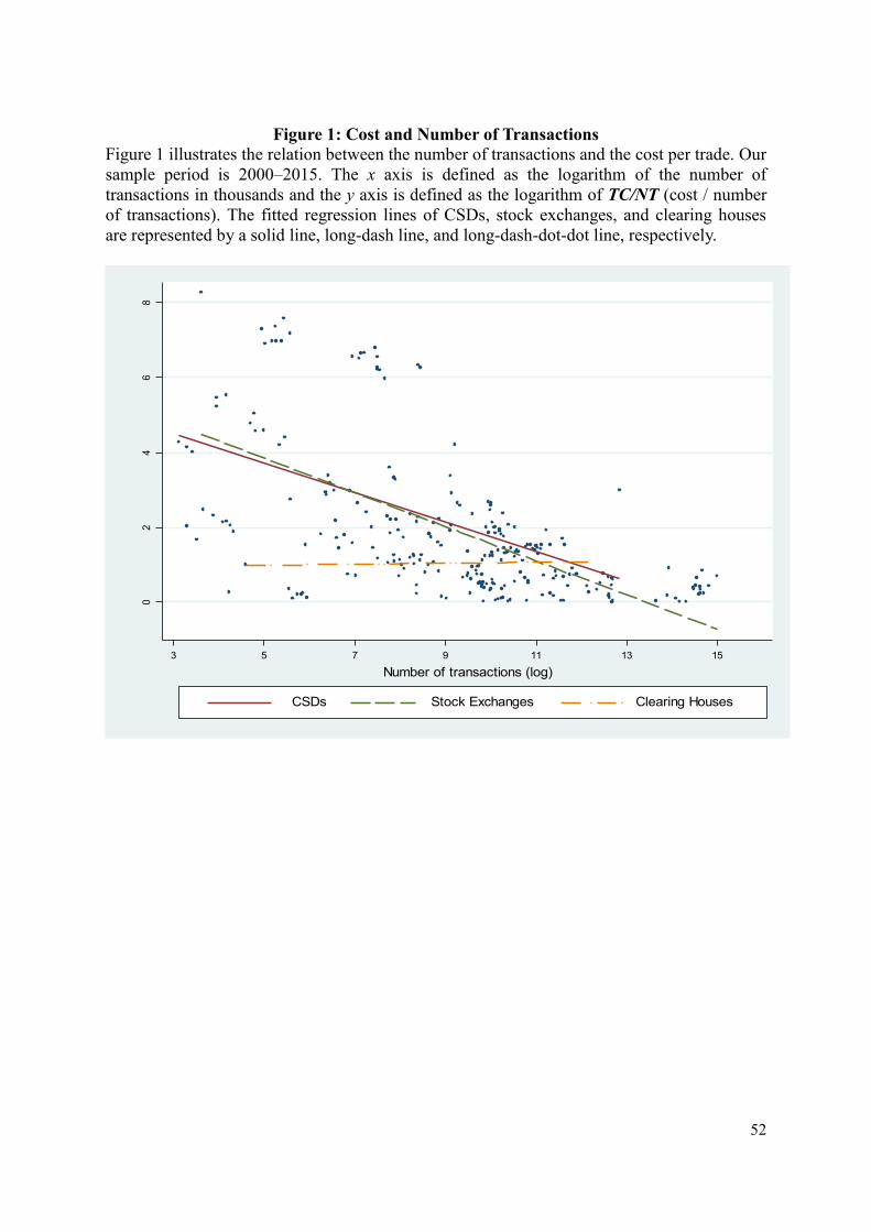
52

Figure 1: Cost and Number of Transactions

Figure 1 illustrates the relation between the number of transactions and the cost per trade. Our

sample period is 2000–2015. The x axis is defined as the logarithm of the number of

transactions in thousands and the y axis is defined as the logarithm of TC/NT (cost / number

of transactions). The fitted regression lines of CSDs, stock exchanges, and clearing houses

are represented by a solid line, long-dash line, and long-dash-dot-dot line, respectively.

02

46

8

Cost

/ n

um

ber

of

transa

ctions

(log)

3 5 7 9 11 13 15

Number of transactions (log)

CSDs Stock Exchanges Clearing Houses

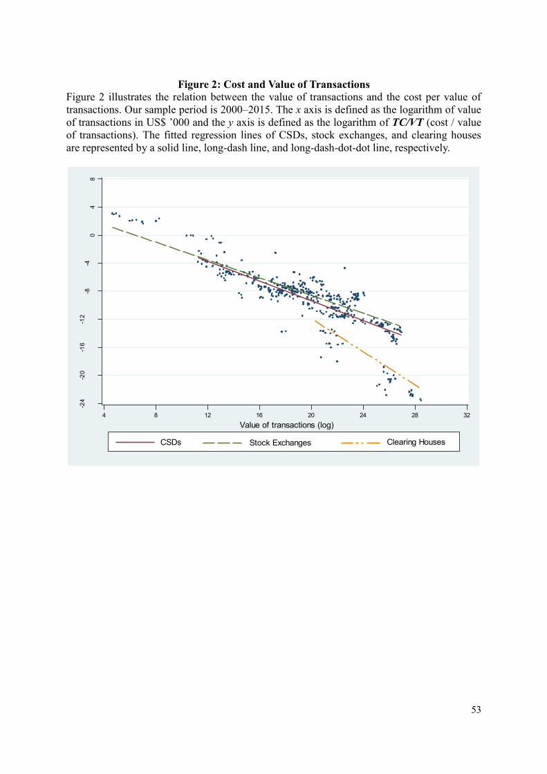
53

Figure 2: Cost and Value of Transactions

Figure 2 illustrates the relation between the value of transactions and the cost per value of

transactions. Our sample period is 2000–2015. The x axis is defined as the logarithm of value

of transactions in US$ ’000 and the y axis is defined as the logarithm of TC/VT (cost / value

of transactions). The fitted regression lines of CSDs, stock exchanges, and clearing houses

are represented by a solid line, long-dash line, and long-dash-dot-dot line, respectively.

-24

-20

-16

-12

-8-4

04

8

Cost

/ valu

e o

f tr

ansactions (

log)

4 8 12 16 20 24 28 32

Value of transactions (log)

CSDs Stock Exchanges Clearing Houses

54

Table A1: Cost Regressed on Output Proxies

This table presents the regressions of the simple loglinear model by using the number of

transactions, NTit (denoted as 𝑸𝒊𝒕𝟏 ), and the value of transactions, VTit (denoted as 𝑸𝒊𝒕

𝟐 )) as

proxies for output. We also include time trend variable t and ICTit (denoted as 𝑷𝒊𝒕𝟐 ) as proxies

for technological development. Our sample period is 2000–2015. The dependent variable

represents the logarithm of total operating costs (𝑻𝑪𝒊𝒕). All regressions are OLS estimations.

The superscripts ***, **, * indicate significance levels of 0.01, 0.05, and 0.10, respectively.

Variables (1) (2) (3) (4) (5)

ln Q1 0.175***

0.115*** 0.113*** 0.139***

(7.64)

(3.90) (3.83) (4.08)

ln Q2 0.286*** 0.331*** 0.330*** 0.221***

(18.72) (20.89) (20.45) (7.12)

t

−0.00386 −0.0280

(−0.18) (−1.24)

ln P2 −0.741***

(−4.81)

Intercept 8.825*** 5.365*** 3.080*** 3.202*** 5.637***

(30.37) (17.43) (7.47) (5.51) (7.79)

N 653 445 401 399 318

R²-adjusted 0.0801 0.404 0.469 0.464 0.489

F-statistic 58.36*** 350.3*** 248.3*** 162.7*** 92.31***

55

Table A2: Full Sample Translog Cost Regression Estimation, including the Single-Input Single-Output Model and Multiple-Inputs, Multiple-Outputs Model This table presents the regressions results of the translog specification as presented in the equation in (1). Our sample period is 2000–2015. Panel A shows the results of translog specifications, including single-input (GDPPCit (denoted as

𝑷𝒊𝒕𝟏 )), single-output (number of transactions, NTit (denoted as 𝑸𝒊𝒕

𝟏 )), year dummy variables, and time trend variable t. Panel B shows the results of translog specifications, including multiple-inputs (GDPPCit (denoted as 𝑷𝒊𝒕𝟏 ) and ICTit

(denoted as 𝑷𝒊𝒕𝟐 )), multiple-outputs (number of transactions, NTit (denoted as 𝑸𝒊𝒕

𝟏 ) and value of transactions VTit (denoted as 𝑸𝒊𝒕𝟐 )), year dummy variables, and time trend variable t. Regressions in Columns (1)–(3) in Panel A and Panel B

are fixed effect estimations that control for the fixed effects of the FMI and cluster the standard errors at each institution; regressions in Columns (4)–(6) in Panel A and Panel B are stochastic frontiers analysis (SFA) estimations.

Heteroskedasticity-robust t-values are reported in parentheses. The cost scale elasticities (mean) in the last row are the mean of cost scale elasticities for the total sample based on different specifications. The superscripts ***, **, *

indicate significance levels of 0.01, 0.05, and 0.10, respectively.

Panel A: Single-input, single-output model Panel B: Multiple-inputs, multiple-outputs model

Variable (1) (2) (3) (4) (5) (6) (1) (2) (3) (4) (5) (6)

ln P1 1.228*** 1.243** 0.953** 1.040*** 1.288*** 1.157*** −2.915* −1.600 −3.355** −2.053* −1.170 −2.018*

(2.92) (2.53) (2.29) (3.25) (3.77) (3.44) (−1.75) (−1.17) (−2.30) (−1.78) (−0.98) (−1.71)

ln Q1 0.140 0.0948 0.158 0.152 0.153 0.201* 0.365 0.146 0.344 0.521* 0.413 0.520*

(0.82) (0.55) (0.89) (1.40) (1.42) (1.84) (0.85) (0.30) (0.79) (1.82) (1.49) (1.82)

ln P1 * ln P1 −0.00325 0.00434 −0.0842 0.0284 0.0164 −0.00166 0.838** 0.524 0.830** 0.319 0.219 0.317

(−0.02) (0.03) (−0.64) (0.29) (0.17) (−0.02) (2.32) (1.44) (2.52) (1.14) (0.76) (1.13)

ln Q1 * ln Q1 0.00413 0.00635 0.00309 0.00282 0.00295 0.000420 0.00735 0.0135 0.00226 −0.00207 0.00995 −0.00185

(0.23) (0.37) (0.17) (0.32) (0.34) (0.05) (0.30) (0.46) (0.09) (−0.13) (0.63) (−0.11)

ln P1 * ln Q1 −0.0256 −0.0206 −0.0257 −0.0258 −0.0331* −0.0375** −0.239** −0.210** −0.227** −0.165*** −0.155*** −0.165***

(−0.87) (−0.73) (−0.89) (−1.40) (−1.80) (−2.00) (−2.31) (−2.18) (−2.16) (−3.81) (−3.73) (−3.82)

t

0.0382**

0.0598* 0.0395 −0.00591

(2.11)

(1.92) (1.17) (−0.17)

ln P2 7.412*** 6.672*** 7.362*** 4.567*** 4.967*** 4.581*** (3.25) (3.60) (3.44) (3.01) (3.33) (3.01) ln Q2 −1.531** −1.242** −1.412** −0.478 −0.467 −0.488 (−2.44) (−2.21) (−2.27) (−1.15) (−1.14) (−1.16) ln P2 * ln P2 0.257 −0.0602 0.128 0.248 0.273 0.252 (0.77) (−0.16) (0.39) (1.21) (1.40) (1.22) ln Q2 * ln Q2 0.0352 0.0262 0.0282 −0.00194 0.00395 −0.00140 (1.37) (1.04) (1.10) (−0.10) (0.20) (−0.07) ln Q2 * ln Q1 0.0250 0.0255 0.0264 0.00724 0.00447 0.00730 (1.48) (1.55) (1.61) (0.64) (0.42) (0.65) ln Q2 * ln P1 0.186* 0.147* 0.187* 0.179*** 0.153*** 0.178*** (1.77) (1.71) (1.83) (3.49) (3.00) (3.45) ln P2 * ln P1 −0.940** −0.905** −1.080** −0.134 −0.176 −0.136 (−2.03) (−2.31) (−2.53) (−0.56) (−0.76) (−0.57) ln P2 * ln Q1 0.0150 −0.00583 0.0125 0.0280 0.0504 0.0281 (0.20) (−0.08) (0.17) (0.49) (0.92) (0.49) ln P2 * ln Q2 −0.238** −0.217** −0.239** −0.202*** −0.237*** −0.202*** (−2.53) (−2.23) (−2.66) (−3.03) (−3.53) (−3.02) Intercept 6.198*** 6.730*** 6.462*** 2.768*** 2.469** 0.928 26.66*** 24.34*** 26.19*** 10.99** −259.5 11.16** (4.61) (4.67) (4.94) (2.83) (2.35) (0.53) (3.29) (3.46) (3.37) (2.29) (.) (2.27)

N 642 642 641 642 642 641 312 312 312 312 312 312 R²-adjusted 0.119 0.144 0.131

0.166 0.171 0.169

F-statistic 7.155*** 4.113*** 7.047***

16.35*** 70.93*** 17.39*** Wald Chi-squared

82.46*** 109.2*** 78.16*** 135.3*** 154.6*** 134.7***

Year Dummy Variables No Yes No No Yes No No Yes No No Yes No

Estimation Method FE FE FE SFA SFA SFA FE FE FE SFA SFA SFA

Cost Scale Elasticities (Mean) 0.1077 0.1033 0.1129 0.1042 0.0835 0.0889 0.2153 0.1502 0.1985 0.2154 0.2262 0.2154

56

Table A3: Subsample Loglinear and Translog Cost Regression Estimation

This table presents the regressions of loglinear and translog cost specifications on the subsample that reports the direct personnel cost in financial statements. Our sample period is 2000–2015. Panel A shows the results of loglinear

and translog specifications by using GDP per capita (GDPPCit (denoted as 𝑷𝒊𝒕𝟏 )) as a measure of labor costs and the number of transactions (GDPPCit (denoted as 𝑸𝒊𝒕

𝟏 )) as output. Panel B shows the results of loglinear and translog

specifications by using personnel cost (STAFFit (denoted as 𝑷𝒊𝒕𝟑 )) as a measure of labor costs and the number of transactions (GDPPCit (denoted as 𝑸𝒊𝒕

𝟏 )) as output. All regressions are stochastic frontiers analysis (SFA) estimation. Heteroskedasticity-robust t-values are reported in parentheses. The cost scale elasticities (mean) in the last row are the mean of cost scale elasticities for the total sample based on different specifications. The superscripts ***, **, *

indicate significance levels of 0.01, 0.05, and 0.10, respectively.

Panel A Panel B

Variables (1) (2) Variables (1) (2) ln P1 0.800*** 0.983** ln P3 0.0898** 0.155

(5.05) (2.41)

(2.49) (0.94)

ln Q1 0.102*** 0.291** ln Q1 0.113*** 0.251***

(4.51) (2.57)

(5.14) (2.70)

ln P1 * ln P1 0.123 ln P3 * ln P3

0.0365*

(1.03)

(1.72)

ln Q1 * ln Q1 −0.00701 ln Q1 * ln Q1

−0.0128

(−0.76)

(−1.38)

ln P1 * ln Q1 −0.0401** ln P3 * ln Q1

0.00715

(−2.09)

(0.59)

Intercept 3.145*** 1.901 Intercept −2594.9*** −1818.7*** (3.06) (1.47) (−7643.26) (−3344.71)

N 500 500 N 500 500 Wald Chi-squared 50.95*** 63.32*** Wald Chi−squared 31.14*** 36.48***

Cost Scale Elasticities (Mean) 0.102 0.0796 0.113 0.0909

57

Table A4: Summary of Institutions in the Sample, 2000–2015

ID Country / Region Name Broad Range of Asset Classes Institution Type Vertical Integration Horizontal Integration

1 France EBA Clearing 0 Clearing House 0 0

2 Netherlands ABN AMRO Clearing Bank NV 1 Clearing House 0 0

3 Hong Kong ABN AMRO Clearing Hong Kong Limited 1 Clearing House 0 0

4 Singapore ABN AMRO Clearing Singapore Pte Ltd 1 Clearing House 0 0

5 Australia ABN AMRO Clearing Sydney Pte Ltd 1 Clearing House 0 0

6 Argentina Argentina Clearing SA 0 Clearing House 0 0

7 Netherlands CITCO Bank Nederland NV 0 Clearing House 0 0

8 Switzerland CLS Group Holdings AG 1 Clearing House 0 0

9 Russia Central Clearing House 0 Clearing House 1 0

10 Luxembourg CETREL SC 0 Clearing House 0 0

11 India Clearing Corporation of India Ltd 0 Clearing House 1 0

12 Luxembourg Clearstream Services SA 0 Clearing House 1 0

13 Germany Eurex Clearing AG 1 Clearing House 1 0

14 Netherlands European Central Counterparty NV 0 Clearing House 0 0

15 Germany European Commodity Clearing AG 1 Clearing House 0 0

16 United States Fixed Income Clearing Corporation # 0 Clearing House 1 from 2003 0

17 Netherlands Fortis Clearing International BV 0 Clearing House 0 0

18 Hong Kong Hong Kong Exchanges And Clearing Limited 1 Clearing House 0 0

19 United Kingdom LCH. Clearnet Group Limited 1 Clearing House 1 0

20 United Kingdom LCH. Clearnet Limited 1 Clearing House 1 0

21 Russia Moscow Clearing Centre 1 Clearing House 1 0

22 Russia National Clearing Centre CJSC JSCB 1 Clearing House 0 0

23 United States National Securities Clearing Corporation 0 Clearing House 1 0

24 France Natixis Paiements SA 0 Clearing House 0 0

25 United States Options Clearing Corporation 1 Clearing House 1 0

26 Germany Swiss Euro Clearing Bank GmbH (SECB) 0 Clearing House 0 0

27 United Kingdom Tradition London Clearing Limited 1 Clearing House 0 0

28 United Kingdom UBS Clearing and Execution Services Limited 1 Clearing House 0 0

29 Russia United Settlement System 0 Clearing House 0 0

30 Greece Athens Exchange Group 1 Stock Exchange 0 0

31 India BSE India Ltd 1 Stock Exchange 1 from 2011 0

32 Brazil BM&F Bovespa 1 Stock Exchange 0 0

33 Hungary Budapest Stock Exchange 1 Stock Exchange 0 0

34 Malaysia Bursa Malaysia 1 Stock Exchange 1 from 2009 0

35 Cyprus Cyprus Stock Exchange 0 Stock Exchange 0 0

36 Germany Deutsche Börse AG 1 Stock Exchange 1 from 2002 1 from 2003

37 France Euronext 1 Stock Exchange 0 1 from 2002

38 Belgium Euronext Brussels 1 Stock Exchange 0 0

38 France Euronext Paris SA 1 Stock Exchange 1 1 from 2007

40 Hong Kong Hong Kong Stock Exchange 1 Stock Exchange 0 0

41 Indonesia Indonesia Stock Exchange 1 Stock Exchange 0 0

42 Turkey Istanbul Stock Exchange 1 Stock Exchange 0 0

43 Jamaica Jamaica Stock Exchange 0 Stock Exchange 0 0

44 South Africa Johannesburg Stock Exchange 1 Stock Exchange 0 0

58

Table A4: Summary of Institutions in the Sample, 2000–2015

ID Country / Region Name Broad Range of Asset Classes Institution Type Vertical Integration Horizontal Integration

45 United Kingdom London Stock Exchange 1 Stock Exchange 1 from 2006 1 from 2003

46 Malta Malta Stock Exchange 0 Stock Exchange 0 0

47 Russia Moscow Exchange 1 Stock Exchange 0 0

48 Oman Muscat Securities Market 0 Stock Exchange 0 0

49 United States NASDAQ 1 Stock Exchange 1 from 2008 1 from 2007

50 United States NYSE 1 Stock Exchange 0 1 from 2007

51 Nigeria Nigerian Stock Exchange 0 Stock Exchange 0 0

52 Czech Republic Praha Stock Exchange 0 Stock Exchange 0 1 from 2008

53 Switzerland SIX Swiss Exchange 1 Stock Exchange 1 from 2014 0

54 Singapore Singapore Exchange 1 Stock Exchange 0 1 from 2010

55 Thailand Stock Exchange of Thailand 1 Stock Exchange 0 0

56 Iran Tehran Stock Exchange 1 Stock Exchange 0 0

57 Israel Tel-Aviv Stock Exchange (TASE) 1 Stock Exchange 0 0

58 Japan Tokyo Stock Exchange (TSE) 0 Stock Exchange 0 1 from 2012

59 Austria Wiener Börse AG – Vienna Stock Exchange 1 Stock Exchange 0 1 from 2008

60 United Kingdom BNP Paribas Securities Services Custody Bank Limited 0 CSD 0 0

61 Brazil BM&F Bovespa 0 CSD 1 0

62 France CACEIS Bank France SA 0 CSD 0 0

63 Luxembourg Cedel International 0 CSD 1 0

64 Bosnia and Herzegovina Central Registry of Securities JSC Banja Luka 0 CSD 0 0

65 Turkey Central Securities Depository of Turkey 1 CSD 1 0

66 Slovakia Central Securities Depository of the Slovak Republic 0 CSD 1 0

67 Germany Clearstream Banking AG Frankfurt 1 CSD 1 0

68 Luxembourg Clearstream International 1 CSD 1 0

69 Belgium Euroclear Bank SA 1 CSD 1 1 from 2001

70 France Euroclear France SA 1 CSD 1 0

71 United Kingdom Euroclear Plc 1 CSD 1 0

72 Belgium Euroclear SA/NV 1 CSD 1 0

73 France IXIS Investor Services SA 0 CSD 0 0

74 Japan Japan Securities Clearing Corporation 1. CSD 1 0

75 Poland KDPW 0 CSD 0 0

76 Russia National Settlement Depository 0 CSD 1 0

77 Austria Oesterreichische Clearingbank AG 0 CSD 0 0

78 Netherlands RBC Dexia Investor Services Netherlands NV 0 CSD 0 0

79 Luxembourg RBC Investor Services Bank SA 0 CSD 0 0

80 Spain RBC Investor Services España SA 0 CSD 0 0

81 Turkey Takasbank 1 CSD 0 0

82 United States The Depository Trust Company 1 CSD 0 1 from 2010

59

Table B1: Cost Scale Elasticities Based on Two-inputs and Four-outputs Model According to Size, Type, Integration, Specialization, and Geographical Location This table presents the mean of cost scale elasticities estimated by using the two-inputs (GDPPCit (𝑷𝒊𝒕

𝟏 ) and ICTit (𝑷𝒊𝒕𝟐 )), four-outputs (Number of transactions (𝑸𝒊𝒕

𝟏 ), Value of transactions (𝑸𝒊𝒕𝟐 ), Number of listed companies / Number of Issuers (𝑸𝒊𝒕

𝟑 )), and Market

capitalization / Securities held on accounts (𝑸𝒊𝒕𝟒 )) and time trend variable t, for the total sample, and various subsamples according to institution size, horizontal and vertical integration, type, specialization, and geographical location. Our sample period is 2010–2015.

We report the cost scale elasticities with respect to the number of transactions (based on a single-input, single-output model as presented in the equation in (5)) in Panel A, and the cost scale elasticities with respect to the number of transactions and the value of

transactions (based on a multiple-inputs, multiple-outputs model as presented in the equation in (4)) in Panel B. Significance of group mean differences: * Significant at the 10% level. ** Significant at the 5% level. *** Significant at the 1% level.

Cost scale elasticities based on two-inputs and four-outputs model including time trend variable t

Category ∂lnTC

𝜕lnQ1

∂lnTC

∂lnQ2

∂lnTC

∂lnQ3

∂lnTC

∂lnQ4

∑∂lnTC

∂lnQi

Total Sample 0.0522 0.1704 0.1109 0.3536 0.6871 Institution Size Quantile 4 (Largest) 0.0419 0.1431 0.0834 0.3306 0.5990 Quantile 3 0.0623 0.1731 0.0988 0.3765 0.7107 Quantile 2 0.0574 0.1888 0.1228 0.3491 0.7181 Quantile 1 (Smallest) 0.0505 0.1749 0.1273 0.3605 0.7131 Top 50% 0.0507 0.1560 0.0901 0.3504 0.6471 Bottom 50% 0.0533 0.1804 0.1255 0.3559 0.7151 Group Mean Difference (Top 50% − Bottom 50%) 0.0026 −0.0244*** −0.0354*** -0.0056 −0.0680***

Type of Integration Horizontally integrated 0.0484 0.1654 0.1072 0.3431 0.6641 Non-horizontally integrated 0.0782 0.2043 0.1356 0.4260 0.8441 Group Mean Difference −0.0298*** −0.0389*** −0.0294*** -0.0829*** −0.1800***

Vertically integrated 0.0487 0.1577 0.1091 0.3433 0.6588 Non-vertically integrated 0.0640 0.2124 0.1166 0.3879 0.7809 Group Mean Difference −0.0153** −0.0548** −0.0075 -0.0446**** −0.1221***

Specialization Broad range of asset classes 0.0423 0.1534 0.1079 0.3177 0.6213 Narrow range of asset classes 0.0556 0.1762 0.1119 0.3662 0.7100 Group Mean Difference −0.0134*** −0.0228*** −0.0040 -0.0484*** −0.0886***

Regions Europe 0.0788 0.2000 0.1090 0.4016 0.7894 North America 0.0454 0.1589 0.1064 0.3420 0.6527 Asia-Pacific 0.1091 0.2065 0.0374 0.4508 0.8037 South America & Africa 0.0659 0.2217 0.1691 0.3697 0.8265

Type of FMI CSDs 0.0465 0.1748 0.1030 0.3636 0.6880

Group Mean Difference between Different Subsamples Top 50% − Bottom 50% −0.0060 −0.0188 -0.0085 -0.0261* -0.0072 Broad range of asset classes − Narrow range of asset classes 0.0052 −0.0153 0.0030 -0.0268** −0.0340 Horizontally integrated − Non-horizontally integrated −0.00384** −0.0225*** -0.0109** -0.0556*** −0.01263*** Vertically integrated − Non-vertically integrated -0.0262*** -0.0565*** 0.0121 -0.0529*** -0.0989***

Stock Exchanges 0.0664 0.1880 0.1034 0.3865 0.7443 Group Mean Difference between Different Subsamples Top 50% − Bottom 50% −0.0271*** −0.0651*** −0.0620*** -0.0797*** −0.2339*** Broad range of asset classes − Narrow range of asset classes −0.0433*** -0.0619*** −0.0451*** -0.0863*** −0.2365*** Horizontally integrated − Non-horizontally integrated −0.0166* −0.0311** −0.0547*** -0.0564*** −0.1587*** Vertically integrated − Non-vertically integrated −0.0370** −0.0373* −0.0125** -0.1069*** −0.1937***

Clearing Houses 0.0430 0.1437 0.1301 0.3017 0.6185 Group Mean Difference between Different Subsamples Top 50% − Bottom 50% 0.0090 -0.0456*** −0.0220*** -0.0309*** −0.0896*** Broad range of asset classes − Narrow range of asset classes -0.0036 0.0131 0.0080 -0.0161** 0.0014 Vertically integrated − Non-vertically integrated 0.0104* -0.0795*** -0.0227** 0.0038 -0.0880***

60

Table B2: Summary Statistics of Efficiency Scores Based on Two-inputs and Four-outputs Model This table presents the means of efficiency scores estimated by using the two-inputs (GDPPCit (𝑷𝒊𝒕

𝟏 ) and ICTit (𝑷𝒊𝒕𝟐 )), four-outputs (Number of transactions (𝑸𝒊𝒕

𝟏 ), Value of transactions (𝑸𝒊𝒕𝟐 ), Number of listed companies / Number of Issuers (𝑸𝒊𝒕

𝟑 )), and Market

capitalization / Securities held on accounts (𝑸𝒊𝒕𝟒 )), for the total sample, and various subsamples according to institution size, horizontal and vertical integration, type, specialization, and geographical location. Our sample period is 2010–2015. TE indicates technical

efficiency, PTE indicates pure technical efficiency, CE indicates cost efficiency based on constant returns to scale technology, CEScope indicates CE purged of scale efficiency, VCE indicates cost efficiency based on variable returns to scale technology, RE indicates

revenue efficiency based on constant returns to scale technology, REScope indicates RE purged of scale efficiency, VRE indicates revenue efficiency based on variable returns to scale technology, SE indicates input-oriented scale efficiency, AE indicates

input-oriented allocative efficiency, PE indicates profit efficiency estimated based on Cooper et al. (2004, Eq. (8.1)), CRS indicates constant returns to scale, VRS indicates variable returns to scale, IRS indicates increasing returns to scale, DRS indicates decreasing

returns to scale. Significance of group mean differences: * Significant at the 10% level. ** Significant at the 5% level. *** Significant at the 1% level.

Panel A: Mean of Efficiency

N TE PTE CE CEScope VCE RE REScope VRE SE AE PE

All 388 0.3972 0.2859 0.3622 0.1817 0.2024 0.2949 0.2624 0.3390 0.2736 0.5482 0.6404

Institution Size Quantile 4 (Largest) 104 0.3836 0.3146 0.4457 0.0386 0.0639 0.2412 0.0439 0.1431 0.1068 0.3762 0.7008 Quantile 3 70 0.3180 0.3301 0.3515 0.2464 0.3086 0.3130 0.1562 0.4038 0.3167 0.5018 0.6809 Quantile 2 94 0.6074 0.3050 0.4354 0.3316 0.2792 0.3996 0.4832 0.5514 0.3568 0.6279 0.5627 Quantile 1 (Smallest) 120 0.2905 0.2203 0.2387 0.1505 0.2004 0.2487 0.3409 0.3045 0.3279 0.6620 0.6251 Top 50% 174 0.3572 0.3208 0.3251 0.1222 0.1624 0.2701 0.0890 0.2480 0.1912 0.4267 0.6928 Bottom 50% 214 0.4297 0.2575 0.4078 0.2301 0.2350 0.3150 0.4034 0.4129 0.3406 0.6470 0.5977

Group Mean Difference −0.0725 0.0633 -0.0827* −0.1079*** −0.0726*** -0.0449 -0.3144 -0.1650*** -0.1494*** -0.2203*** 0.0951**

Type of Integration Horizontally integrated 50 0.4591 0.2983 0.2912 0.0109 0.1444 0.3017 0.4315 0.4329 0.1849 0.7385 0.5369 Non-horizontally integrated 338 0.3880 0.2841 0.3727 0.2070 0.2110 0.2939 0.2374 0.3251 0.2867 0.5201 0.6557

Group Mean Difference 0.0711 −0.0413 -0.0815 -0.1961*** -0.0667 0.0078 0.1941*** 0.1078 0.1018* −0.2184*** -0.1187* Vertically integrated 84 0.5602 0.3411 0.3818 0.1584 0.2422 0.4075 0.4822 0.4146 0.2572 0.7394 0.5374 Non-vertically integrated 304 0.3522 0.2707 0.3568 0.1881 0.1914 0.2638 0.2017 0.3181 0.2781 0.4954 0.6688

Group Mean Difference 0.0280 0.0704 0.0250 -0.0297 0.0508 0.1437*** 0.2805*** 0.0964* −0.0209 0.0440*** -0.1315***

Specialization Broad range of asset classes 287 0.3902 0.2851 0.3609 0.1653 0.1811 0. 2362 0.2069 0.3415 0.2771 0.5850 0.6510 Narrow range of asset classes 101 0.4172 0.2883 0.3658 0.2283 0.2630 0. 3155 0. 2820 0.3317 0.2637 0.4438 0.6103

Group Mean Difference -0.0270 −0.0032 −0.0049 -0.0629 -0.0818* -0.0792* -0.0750* 0.0098 0.0134 −0.1412** −0.0407

Region Europe 253 0.1409 0.1303 0.3626 0.2294 0.2105 0.1814 0.2116 0.2936 0.2927 0.4012 0.7667 North America 39 0.9413 0.5633 0.3193 0.1294 0.3005 0.5023 0.5898 0.4614 0.4091 0.8992 0.4372 Asia-Pacific 76 0.7303 0.5261 0.3919 0.0893 0.1561 0.5043 0.2592 0.4521 0.1890 0.7517 0.4486 South America & Africa 29 0.7684 0.7934 0.5466 0.0216 0.1227 0.5122 0.2034 0.2399 0.0614 0.9002 0.1839

Type of FMI Stock Exchanges 163 0.6632 0.4023 0.4247 0.0455 0.1156 0.3726 0.2640 0.3752 0.1366 0.6223 0.5353 Group Mean Difference between Different Subsamples

Top 50% − Bottom 50% 0.2903 −0.0033 −0.0782 −0.0139 -0.0192 0.0647 0.3886*** 0.3335*** -0.0271 −0.3009*** −0.2114*** Broad range of asset classes − Narrow range of asset classes −0.1356 −0.0438 −0.0215 0.0552*** 0.1037*** 0.0793 0.3175*** 0.3531 0.1612*** 0.1442 0.1282 Horizontally integrated − Non-horizontally integrated −0.2169 −0.1323* −0.1439 -0.0462* 0.0461 -0.1217* 0.2104*** 0.0848 0.0851 0.01205 −0.0356 Vertically integrated − Non-vertically integrated

0.1339 0.0142 -0.0275 -0.0444 0.1128 0.0594 0.3380*** 0.3051*** 0.0320 0.3309*** -0.1581* CSDs 118 0.0810 0.1686 0.3959 0.1358 0.1620 0.2649 0.2992 0.2463 0.1970 0.4872 0.6733 Group Mean Difference between Different Subsamples

Top 50% − Bottom 50% -0.0752 0.0197 −0.2744*** 0.0453 0.2012*** 0.0943 0.2600*** 0.1813** -0.0838 −0.1891** -0.1306* Broad range of asset classes − Narrow range of asset classes 0.1068*** 0.2268*** 0.0211 −0.0784 -0.0432 0.2842*** −0.1362* -0.1384 −0.0020 −0.2299** −0.1026 Horizontally integrated − Non-horizontally integrated -0.0475 -0.0589* -0.3853*** −0.1415*** −0.0615 0.2000 0.2816 0.1603 −0.1377* −0.5355*** -0.3683*** Vertically integrated − Non-vertically integrated

-0.0392 0.0211*** 0.0601 0.1020 0.0130 0.0348 0.1796* 0.0746 0.0458 0.1972* -0.0558 Clearing Houses 107 0.3407 0.2380 0.2298 0.4398 0.3793 0.2095 0.2195 0.3860 0.5669 0.5028 0.7642 Group Mean Difference between Different Subsamples

Top 50% − Bottom 50% 0.4278** 0.0355 0.0428 −0.2203** −0.3464*** 0.2344*** 0.2076*** -0.0512 -0.0706 0.3408*** -0.1935*** Broad range of asset classes − Narrow range of asset classes −0.2227 −0.2612*** −0.1151 0.0389 −0.1629* −0.1835** −0.2235** −0.1746* 0.1139 0.0098 0.2126** Vertically integrated − Non-vertically integrated

0.5696** 0.2162** 0.1321 -0.2832*** -0.0872 0.3842*** 0.3428*** -0.1113 0.3087*** 0.2438** -0.2565***

Documents

Forthcoming in the Journal of International Financial ... · Forthcoming in the Journal of International Financial Markets, Institutions & Money September 13, 2017 Economies of Scale