P-03-43

Svensk Kärnbränslehantering ABSwedish Nuclear Fueland Waste Management CoBox 5864SE-102 40 Stockholm SwedenTel 08-459 84 00

+46 8 459 84 00Fax 08-661 57 19

+46 8 661 57 19

Forsmark site investigation

Ground penetrating radar andresistivity measurements foroverburden investigations

Johan Nissen, Malå Geoscience AB

April 2003

ISSN 1651-4416

SKB P-03-43

Forsmark site investigation

Ground penetrating radar andresistivity measurements foroverburden investigations

Johan Nissen, Malå Geoscience AB

April 2003

Keywords: Ground penetrating radar, GPS, resistivity measurements, CVES,overburden investigations

This report concerns a study which was conducted in part for SKB. Theconclusions and viewpoints presented in the report are those of the author(s)and do not necessarily coincide with those of the client.

A pdf version of this document can be downloaded from www.skb.se

3

Contents

1 Introduction 5

2 Objective and scope 7

3 Measuring procedure and equipment 93.1 Resistivity measurements 93.2 Positioning 103.3 Radar measurements 11

4 Results and data delivery 134.1 Resistivity measurements 13

4.1.1 Profile 1 (LFM000568) 134.1.2 Profiles 2, 3 and 4 (LFM000569, 570 and 571) 17

4.2 Radar measurements 214.2.1 Profile 1 (LFM000568) 214.2.2 Profiles 2, 3, 4A and 7 (LFM000569, 570, 572 and 575) 214.2.3 Profiles 5 and 6 (LFM000573 and 574) 23

4.3 Conclusions 25

5 References 27

Appendix 1 – Coordinates along the survey profiles 29

5

1 Introduction

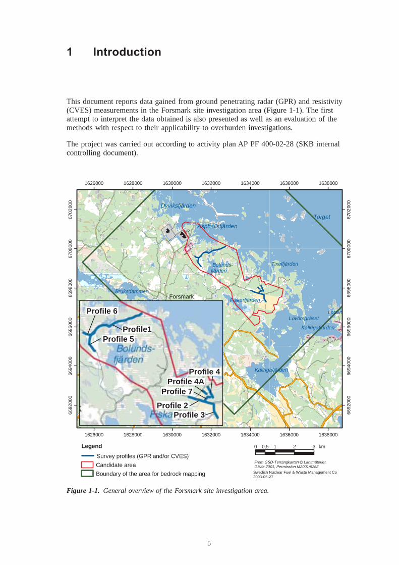
This document reports data gained from ground penetrating radar (GPR) and resistivity(CVES) measurements in the Forsmark site investigation area (Figure 1-1). The firstattempt to interpret the data obtained is also presented as well as an evaluation of themethods with respect to their applicability to overburden investigations.

The project was carried out according to activity plan AP PF 400-02-28 (SKB internalcontrolling document).

Figure 1-1. General overview of the Forsmark site investigation area.

Torget

Dyviksfjärden

Asphällsfjärden

Lotten

Tixelfjärden

L v rsgr set

Kallrigafjärden

Kallrigafjärden

fjärdenBolunds-

Bruksdammen

FiskarfjärdenForsmark

1626000

1626000

1628000

1628000

1630000

1630000

1632000

1632000

1634000

1634000

1636000

1636000

1638000

1638000

6692

000

6692

000

6694

000

6694

000

6696

000

6696

000

6698

000

6698

000

6700

000

6700

000

6702

000

6702

000

0 1 2 30,5 km

From GSD-Terr ngkartan Lantm terietG vle 2001, Permission M2001/5268Swedish Nuclear Fuel & Waste Management Co2003-05-27

Legend

Survey profiles (GPR and/or CVES)

Candidate area

Boundary of the area for bedrock mapping

öö ä

ä ää

c

Profile1Profile 5

Profile 6

Profile 2Profile 3

Profile 4Profile 4A

Profile 7

7

2 Objective and scope

The objective of the survey was to perform test measurements with two geophysicalmethods, which were considered to have a potential for future application to overburdeninvestigations in the Forsmark area.

The measurements were carried out during October 2002–January 2003 along eightprofiles (Figure 1-1). Three profiles were investigated with both methods, one with CVESonly and four with GPR only.

9

3 Measuring procedure and equipment

The profiles measured have been denoted Profile 1 to Profile 7 and these denotations areconsequently used in the raw data files. The corresponding SKB ID-codes are as follows:

Profile 1 LFM000568 (CVES, GPR(minor part))

2 LFM000569 (CVES, GPR)

3 LFM000570 (CVES, GPR)

4 LFM000571 (CVES)

4A LFM000572 (GPR)

5 LFM000573 (GPR)

6 LFM000574 (GPR)

7 LFM000575 (GPR)

In this report, the “field names” (Profile 1–7) are used, frequently complemented by theSKB ID-codes.

3.1 Resistivity measurementsMeasurements with CVES (Continuous Vertical Electrical Sounding) were conductedwith 5 m electrode separations along the Profiles 1–3 and with 2 m electrode separationsalong Profile 4 (Figure 1-1).

The data was collected with the following equipment:

Profile 1,2,3 ABEM Terrameter SAS 4000, S/N 2982231 Cable system, 5 m

Profile 4 ABEM Terrameter SAS 1000, S/N 2020281 Cable system, 2 m

For all readings, the equipment was set to perform a maximum of 4 stackings, with thecondition that if the deviation between the first two readings was below 1% the stackingprocedure was stopped. The error displayed is the deviation in percent between the tworeadings. If more than two stackings are performed, the resulting error is calculated asthe standard deviation.

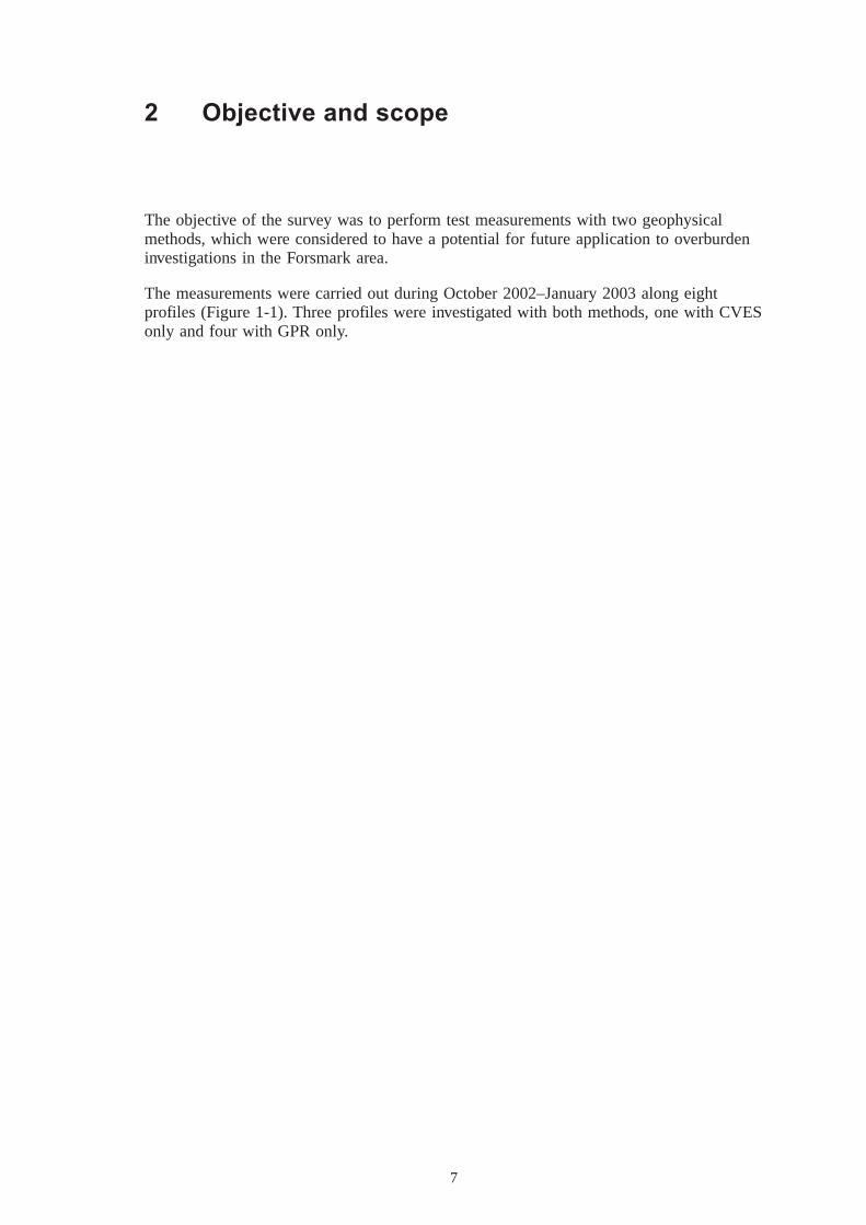
Along all profiles, the data quality was good. In Figure 3-1, the error distribution for all1809 readings from Profile 1 is demonstrated. As can be seen, the typical error is in theinterval 0.1%–0.2%. 95% of all readings has a standard deviation less than 0.3%.

10

3.2 PositioningA GPS reading was taken at each cable joint (i.e. for each 100 m in Profile 1–3 and each40 m in Profile 4). The GPS instrument was checked on four local fix points in the area.Table 3-1 comprises the checks. It is seen that the deviation is within a few metres.

Figure 3-1. Distribution of error in CVES measurements, Profile 1.

Error distribution (profile 1)

0

400

800

1200

1600

0 0.4 0.8 1.2 1.6 2

Error in %

Fre

qu

en

cy

0%

25%

50%

75%

100%

Frequency

Table 3-1. GPS readings at four local fix points, and the corresponding referencevalues from GEOCON /1/.

ID Measured position GEOCON

1102 16313336699422 16313336699418

1105 16346536697860 16346526697858

1106 16345676697872 16345656697871

1107 16344116698013 16344126698014

11

3.3 Radar measurementsAll radar measurements were conducted with the Malå Geoscience RAMAC unshielded50 MHz antennas and a CUII control unit. The data presented in this report is processedby means of the program REFLEXW, and the following processing steps were made:

1. Adjust time zero.

2. Remove DC shift.

3. Band pass filtering (Butterworth) 25–100 MHz.

4. Gain adjustment for display.

13

4 Results and data delivery

The obtained results from the investigation are presented below. The raw and processed/interpreted data have been delivered on a CD to SKB. Information on the activity hasbeen inserted in the SICADA database, whereas the delivered CD has been archived.It is foreseen that further interpretation, including input data from e.g. drilling, will bemade in several steps. These future interpretations will be inserted in SICADA.

The SICADA reference to the present activity is Field note Forsmark 108.

4.1 Resistivity measurements4.1.1 Profile 1 (LFM000568)

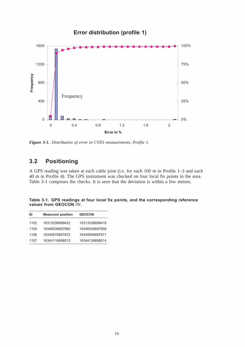
Profile 1 was measured from east to west along the existing path of a seismic line, seeFigure 4-1. At each cable joint (every 100 m) the position corresponding to the existingseismic line was noted. These positions are indicated in the interpretation. The positionsof all cable joints are given in Appendix 1.

The CVES-data (Figure 4-2 a,b) is presented after an inversion procedure with theprogram RES2DINV, version 3.4. Topography data from the seismic survey is includedin the interpretation.

Figure 4-1. Profile 1 (LFM000568). The yellow arrows show the route from the GPS readings.

14

Figure 4-2a. Profile 1 (LFM000568). Resistivity sections.

15

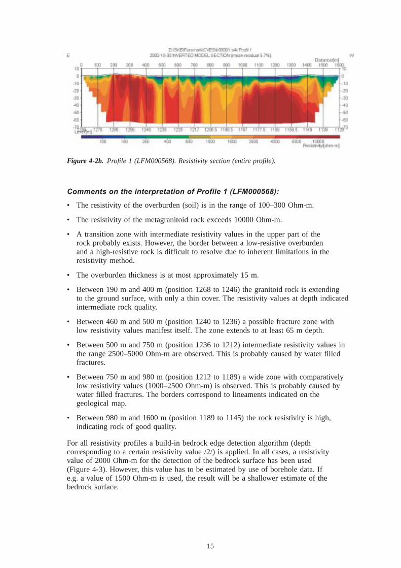
Comments on the interpretation of Profile 1 (LFM000568):

• The resistivity of the overburden (soil) is in the range of 100–300 Ohm-m.

• The resistivity of the metagranitoid rock exceeds 10000 Ohm-m.

• A transition zone with intermediate resistivity values in the upper part of therock probably exists. However, the border between a low-resistive overburdenand a high-resistive rock is difficult to resolve due to inherent limitations in theresistivity method.

• The overburden thickness is at most approximately 15 m.

• Between 190 m and 400 m (position 1268 to 1246) the granitoid rock is extendingto the ground surface, with only a thin cover. The resistivity values at depth indicatedintermediate rock quality.

• Between 460 m and 500 m (position 1240 to 1236) a possible fracture zone withlow resistivity values manifest itself. The zone extends to at least 65 m depth.

• Between 500 m and 750 m (position 1236 to 1212) intermediate resistivity values inthe range 2500–5000 Ohm-m are observed. This is probably caused by water filledfractures.

• Between 750 m and 980 m (position 1212 to 1189) a wide zone with comparativelylow resistivity values (1000–2500 Ohm-m) is observed. This is probably caused bywater filled fractures. The borders correspond to lineaments indicated on thegeological map.

• Between 980 m and 1600 m (position 1189 to 1145) the rock resistivity is high,indicating rock of good quality.

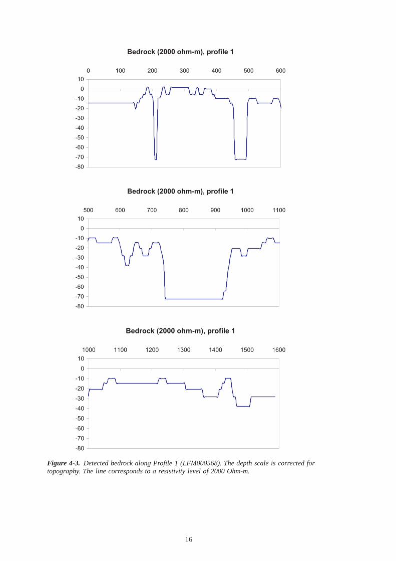
For all resistivity profiles a build-in bedrock edge detection algorithm (depthcorresponding to a certain resistivity value /2/) is applied. In all cases, a resistivityvalue of 2000 Ohm-m for the detection of the bedrock surface has been used(Figure 4-3). However, this value has to be estimated by use of borehole data. Ife.g. a value of 1500 Ohm-m is used, the result will be a shallower estimate of thebedrock surface.

Figure 4-2b. Profile 1 (LFM000568). Resistivity section (entire profile).

16

Figure 4-3. Detected bedrock along Profile 1 (LFM000568). The depth scale is corrected fortopography. The line corresponds to a resistivity level of 2000 Ohm-m.

Bedrock (2000 ohm-m), profile 1

-80

-70

-60

-50

-40

-30

-20

-10

0

10

0 100 200 300 400 500 600

Bedrock (2000 ohm-m), profile 1

-80

-70

-60

-50

-40

-30

-20

-10

0

10

500 600 700 800 900 1000 1100

Bedrock (2000 ohm-m), profile 1

-80

-70

-60

-50

-40

-30

-20

-10

0

10

1000 1100 1200 1300 1400 1500 1600

17

4.1.2 Profiles 2, 3 and 4 (LFM000569, 570 and 571)

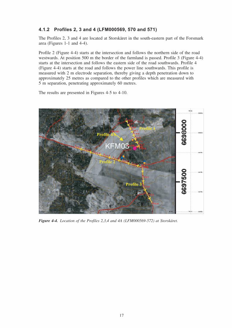
The Profiles 2, 3 and 4 are located at Storskäret in the south-eastern part of the Forsmarkarea (Figures 1-1 and 4-4).

Profile 2 (Figure 4-4) starts at the intersection and follows the northern side of the roadwestwards. At position 500 m the border of the farmland is passed. Profile 3 (Figure 4-4)starts at the intersection and follows the eastern side of the road southwards. Profile 4(Figure 4-4) starts at the road and follows the power line southwards. This profile ismeasured with 2 m electrode separation, thereby giving a depth penetration down toapproximately 25 metres as compared to the other profiles which are measured with5 m separation, penetrating approximately 60 metres.

The results are presented in Figures 4-5 to 4-10.

Figure 4-4. Location of the Profiles 2,3,4 and 4A (LFM000569-572) at Storskäret.

Profile 2

Profile 3

Profile 4

Profile 4A

18

Comments on the interpretation of Profile 2 (LFM000569):

• The overburden thickness varies from 2–3 m (at position 130 m) to at least 20 m(at position 350 m).

• Between 310 m and 450 m a low-resistivity zone, probably a fracture zone, isobserved.

• In general the rock resistivity values are high, indicating rock without fracturesor fissures.

Figure 4-5. Profile 2 (LFM000569). Resistivity section.

Figure 4-6. Detected bedrock in Profile 2 (LFM000569). The depth scale is corrected fortopography. The line corresponds to a resistivity level of 2000 Ohm-m.

Bedrock (2000 ohm-m), profile 2

-40

-35

-30

-25

-20

-15

-10

-5

0

0 100 200 300 400 500 600 700

19

Comments on the interpretation of Profile 3 (LFM000570):

An area of low resistivity is observed between 150 m and 250 m. This may indicatea section of fractured bedrock. However, the profile is rather short for making definiteconclusions.

Figure 4-7. Profile 3 (LFM000570). Resistivity section.

Figure 4-8. Detected bedrock in Profile 3 (LFM000570). The depth scale is corrected fortopography. The line corresponds to a resistivity level of 2000 Ohm-m.

Bedrock (2000 ohm-m), profile 3

-50

-45

-40

-35

-30

-25

-20

-15

-10

-5

0

0 50 100 150 200 250 300 350 400

20

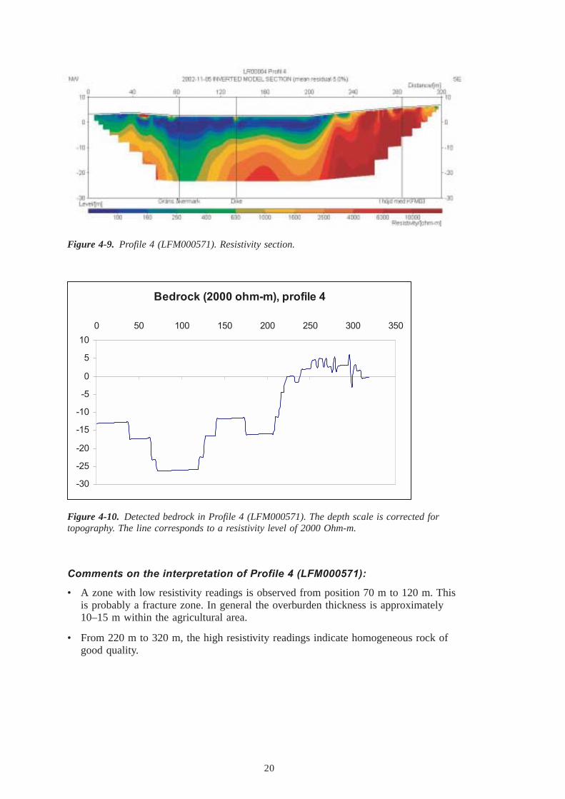
Comments on the interpretation of Profile 4 (LFM000571):

• A zone with low resistivity readings is observed from position 70 m to 120 m. Thisis probably a fracture zone. In general the overburden thickness is approximately10–15 m within the agricultural area.

• From 220 m to 320 m, the high resistivity readings indicate homogeneous rock ofgood quality.

Figure 4-9. Profile 4 (LFM000571). Resistivity section.

Figure 4-10. Detected bedrock in Profile 4 (LFM000571). The depth scale is corrected fortopography. The line corresponds to a resistivity level of 2000 Ohm-m.

Bedrock (2000 ohm-m), profile 4

-30

-25

-20

-15

-10

-5

0

5

10

0 50 100 150 200 250 300 350

21

4.2 Radar measurements4.2.1 Profile 1 (LFM000568)

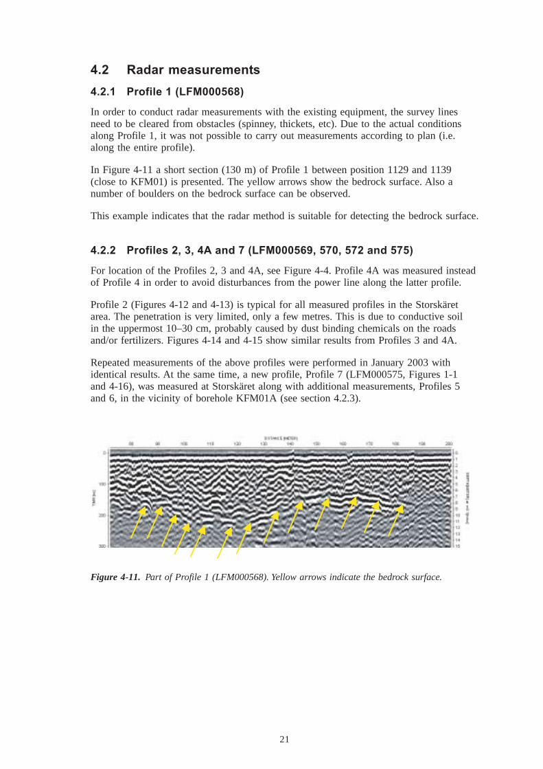
In order to conduct radar measurements with the existing equipment, the survey linesneed to be cleared from obstacles (spinney, thickets, etc). Due to the actual conditionsalong Profile 1, it was not possible to carry out measurements according to plan (i.e.along the entire profile).

In Figure 4-11 a short section (130 m) of Profile 1 between position 1129 and 1139(close to KFM01) is presented. The yellow arrows show the bedrock surface. Also anumber of boulders on the bedrock surface can be observed.

This example indicates that the radar method is suitable for detecting the bedrock surface.

4.2.2 Profiles 2, 3, 4A and 7 (LFM000569, 570, 572 and 575)

For location of the Profiles 2, 3 and 4A, see Figure 4-4. Profile 4A was measured insteadof Profile 4 in order to avoid disturbances from the power line along the latter profile.

Profile 2 (Figures 4-12 and 4-13) is typical for all measured profiles in the Storskäretarea. The penetration is very limited, only a few metres. This is due to conductive soilin the uppermost 10–30 cm, probably caused by dust binding chemicals on the roadsand/or fertilizers. Figures 4-14 and 4-15 show similar results from Profiles 3 and 4A.

Repeated measurements of the above profiles were performed in January 2003 withidentical results. At the same time, a new profile, Profile 7 (LFM000575, Figures 1-1and 4-16), was measured at Storskäret along with additional measurements, Profiles 5and 6, in the vicinity of borehole KFM01A (see section 4.2.3).

Figure 4-11. Part of Profile 1 (LFM000568). Yellow arrows indicate the bedrock surface.

22

Figure 4-12. Radar data from Profile 2 (LFM000569). The hyperbolic signatures are caused byair reflections from trees and a building.

Figure 4-13. Enhanced view of a section of Profile 2 (LFM000569). The end of the agriculturalarea is at position 500 m. It is seen that there is essentially no penetration. The hyperbolicstructures correspond to air-reflections from a fence and from trees.

Figure 4-14. Profile 3 (LFM000570). The hyperbolic signatures are caused by air reflectionsfrom trees, power lines and buildings.

23

4.2.3 Profiles 5 and 6 (LFM000573 and 574)

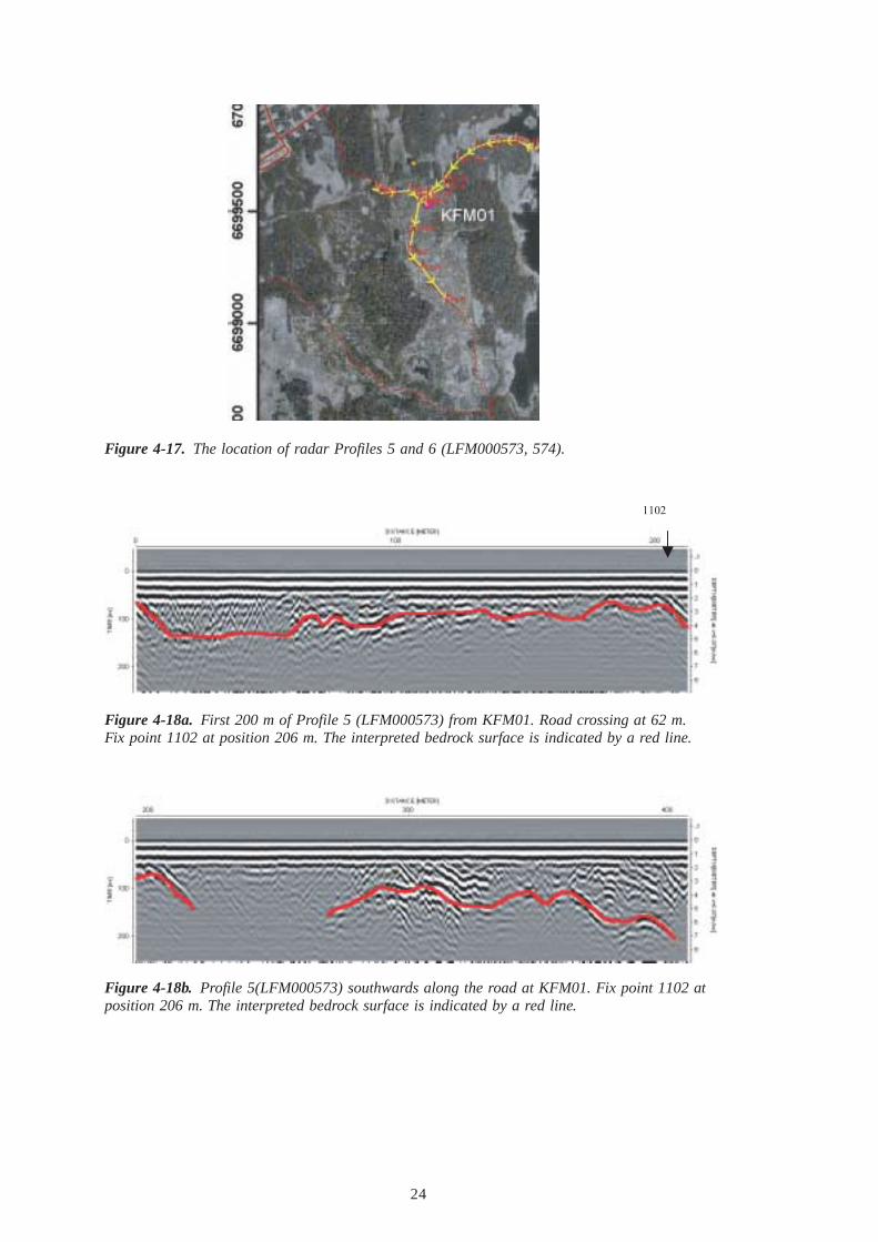
Figure 4-17 shows the location of the Profiles 5 and 6, see also Figure 1-1.

Figures 4-18 a–c present the results from Profile 5 along the road, starting at the fence atKFM01, passing the road crossing at 62 m and extending southwards. The red line in thefigures corresponds to the interpreted bedrock surface.

Figure 4-19 presents the results from Profile 6 (LFM000574) measured along the roadnearby KFM01. The profile starts at the power line, passes KFM01 and extends along asmall road to SFM0003. It is seen that the filling material on the new road from KFM01to SFM0003 screens the radar-wave.

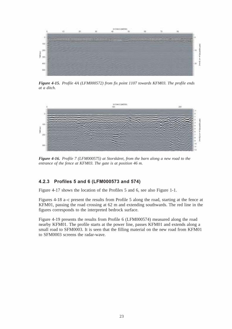
Figure 4-15. Profile 4A (LFM000572) from fix point 1107 towards KFM03. The profile endsat a ditch.

Figure 4-16. Profile 7 (LFM000575) at Storskäret, from the barn along a new road to theentrance of the fence at KFM03. The gate is at position 46 m.

24

Figure 4-17. The location of radar Profiles 5 and 6 (LFM000573, 574).

Figure 4-18a. First 200 m of Profile 5 (LFM000573) from KFM01. Road crossing at 62 m.Fix point 1102 at position 206 m. The interpreted bedrock surface is indicated by a red line.

Figure 4-18b. Profile 5(LFM000573) southwards along the road at KFM01. Fix point 1102 atposition 206 m. The interpreted bedrock surface is indicated by a red line.

1102

25

4.3 ConclusionsThe present study has demonstrated that CVES measurements may give a goodpicture of the structure of the overburden and the upper part of the bedrock. It wasalso demonstrated that it is possible to achieve data of very good quality. An inherentdisadvantage of the resistivity method is, however, its limited resolution of the depthto a resistive basement.

According to the CVES measurements, the overall resistivity of the overburden isaround 100 Ohm-m, which indicates that it should be possible to conduct successfulradar measurements. This is also clearly demonstrated from the very short radar sectionof Profile 1 and from the profiles close to KFM01. The radar method is seen to be wellsuited mainly for mapping the overburden thickness.

However, in the arable land around Storskäret many decades of farming havemost probably created a zone of low resistivity near the surface, which makesradar measurements more or less impossible. Similarly, the use of dust-bindingchemicals causes the conductivity to increase, thus making it difficult to performradar measurements along the roads.

Figure 4-18c. Last part of Profile 5 (LFM000573), ending at the turnaround at position 550 m.The interpreted bedrock surface is indicated by a red line.

Figure 4-19. Profile 6 (LFM000574) along road, starting at power line, passing KFM01,extending along small road. Stop at SFM0003. Passing road intersection at 135 m and passingKFM01 at 195 m. The interpreted bedrock surface is indicated by a red line.

27

5 References

/1/ GEOCON, 2002. Stomnätsmätning i plan och höjd vid PLU Forsmark.Rapport S1020.

/2/ GEOTOMO Software, 2003. RES2DINV ver 3.51 Reference Manual.

29

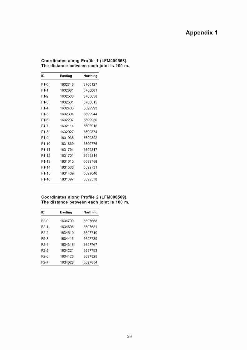
Appendix 1

Coordinates along Profile 1 (LFM000568).The distance between each joint is 100 m.

ID Easting Northing

F1-0 1632746 6700127

F1-1 1632681 6700081

F1-2 1632588 6700058

F1-3 1632501 6700015

F1-4 1632403 6699993

F1-5 1632304 6699944

F1-6 1632207 6699930

F1-7 1632114 6699916

F1-8 1632027 6699874

F1-9 1631938 6699822

F1-10 1631869 6699776

F1-11 1631794 6699817

F1-12 1631701 6699814

F1-13 1631610 6699788

F1-14 1631536 6699731

F1-15 1631469 6699646

F1-16 1631397 6699578

Coordinates along Profile 2 (LFM000569).The distance between each joint is 100 m.

ID Easting Northing

F2-0 1634700 6697658

F2-1 1634606 6697681

F2-2 1634510 6697710

F2-3 1634413 6697739

F2-4 1634318 6697767

F2-5 1634221 6697793

F2-6 1634126 6697825

F2-7 1634028 6697854

30

Coordinates along Profile 4 (LFM000671).The distance between each joint is 40 m.

ID Easting Northing

F4-0 1634548 6698128

F4-1 1634563 6698093

F4-2 1634582 6698056

F4-3 1634601 6698022

F4-4 1634617 6697990

F4-5 1634633 6697950

F4-6 1634649 6697915

F4-7 1634669 6697879

F4-8 1634684 6697841

Coordinates along Profile 4A (LFM000672).

ID Easting Northing

F4A-0 1634412 6698014

F4A-1 1634517 6697931

Coordinates along Profile 5 (LFM000673).

ID Easting Northing

F5-0 1631381 6699542

F5-1 1631349 6699541

F5-2 1631357 6699496

F5-3 1631333 6699418

F5-4 1631319 6699295

F5-5 1631384 6699224

F5-6 1631457 6699117

F5-7 1631481 6699107

Coordinates along Profile 3 (LFM000570).The distance between each joint is 100 m.

ID Easting Northing

F3-0 1634711 6697649

F3-1 1634716 6697550

F3-2 1634723 6697453

F3-3 1634765 6697371

F3-4 1634813 6697282

31

Coordinates along Profile 6 (LFM000674).

ID Easting Northing

F6-0 1631173 6699607

F6-1 1631230 6699575

F6-2 1631340 6699550

F6-3 1631385 6699554

F6-4 1631434 6699580

F5-5 1631474 6699616

Coordinates along Profile 7 (LFM000675).

ID Easting Northing

F7-0 1634455 6697734

F7-1 1634544 6697850

F7-2 1634607 6697845