Formulating Models of Simple Systems

D-4697-2

Formulating Models of Simple Systems

using

Vensim PLEversion 3.0B

Professor Nelson RepenningSystem Dynamics Group

MIT Sloan School of ManagementCambridge, MA O2142

Edited by Laura Black, Farzana S. Mohamed, and students in the System Dynamics in EducationProject, April 1998.

Copyright © 1998 by the Massachusetts Institute of Technology.

D-4697-2

I. Introduction and Getting Started 2

I. Introduction and Getting Started

The purpose of this tutorial is to help you develop some familiarity with building and analyzingsystem dynamics models using the Vensim PLE software. In order to become familiar withVensim PLE, you are going to build a simple model of the federal deficit.

To begin you need to get Vensim PLE ready for modeling. This tutorial makes use of theMacintosh version on Vensim PLE; the IBM-Compatible version should work similarly, but someof the screens may look different. When you first open Vensim PLE on your computer, the screenshould look like this:

To start working on a new model go to the File menu and select New Model. Vensim PLE willreturn the following dialog box:

D-4697-2


To begin your effort you must choose the time horizon of your model (when your simulation willstart and finish), the appropriate time step (how accurately you wish to simulate your model), andthe units of time. Start your model of the deficit in 1988 (enter 1988 in the INITIAL TIME box)and simulate it through the year 2010. Select a time step of 0.25 years. Finally, change theunits of time from Month to Year. Your dialog box should now look like this:

Click on OK or hit return. To give your model a name, choose the Save As... command from theFile menu and enter the desired name in the text field and click on OK. (Vensim PLE shouldautomatically supply the .mdl extension. If you are working with a different version of Vensimand see a Show all of type option on the right side of the dialog box, make sure that the .mdl FmtModels extension is selected. This allows Vensim PLE to save the model in a format that can beused by both Macintosh and IBM-compatible computers.)∗

∗ Vensim saves every simulation run and custom graph you produce as a separate file. It supplies a .vdf

extension for simulation runs. These files cannot be opened from outside the Vensim application; they can beopened from inside Vensim through the Datasets / Simulate Model.. . and Control / Custom Graphsdialog boxes.

D-4697-2


Your screen should now look like this:

You are ready to start building your model.

D-4697-2

II. Developing the Stock, Flow, and Feedback Structure 5

II. Developing the Stock, Flow, and Feedback Structure

The Vensim PLE software is designed using the metaphor of a “work bench.” The large blankarea in the middle of the screen is your work area, where you actually develop and analyze yourmodel. The different buttons on the border of the work area represent the different “tools”available as you work on your model. The upper toolbar consists of the Title Bar, a Menu, a MainToolbar, and Sketch Tools. The Main Toolbar comprises two sets of tools: file operation tools thatcontrol standard file functions—opening, closing and saving files, printing, cutting, copying, andpasting—as well as simulation and graphing tools that will allow you to set up and runsimulations, and set up display graphs. The sketch tools allow you to build in model components.The tools on the Status Bar (the bottom of the window) allow you to change the formatting of thediagram. The Analysis Tools on the left on the window are tools that you will use to analyze yourmodel to understand its behavior. You will become familiar with many of these tools as you buildthe deficit model.

To begin, add a stock representing the outstanding federal debt to your model. Click on the button (the one with the box in it) on the sketch tools bar and then click in the right center of thescreen. You use this tool whenever you want to add a stock (also known as a level) variable toyour model. Vensim PLE then returns an empty text box and a blinking cursor. Type the wordDebt and then hit the return key.

D-4697-2



You have just created the first variable in your model, the stock of money that constitutes thefederal debt.

Now, add the inflow to the stock of Debt. Click on the button on the sketch tools bar.Now, click and release once to the left of the Debt stock, move the cursor so that it sits inside theDebt stock, (the stock should “blacken” if you do this correctly) and click and release again.Vensim PLE then gives you an empty text box and a blinking cursor. Type Net Federal Deficitand hit the return key.

D-4697-2



Note: The icon (which is supposed to resemble a cloud) represents the boundary of yourmodel. In this case the “cloud” on the left side of the flow signifies that you do not, at themoment, care about where the deficit comes from — you are not keeping track of the stock that isbeing drained by the deficit flow. You do care, however, where the deficit goes: hence, you areaccumulating the deficit in the Debt stock. If your deficit flow has “clouds” on both ends, then

you have not hooked the flow to the stock correctly. To fix this problem, click on the tool andthen click on the flow valve. This action will remove the flow from the model and let you startover again.

You have now created the flow, Net Federal Deficit, which increases the stock of Debt.At this point you may you wish to change the name of the stock variable from Debt to Federal

Debt. Click on the button (the one without the box in it) on the sketch tool bar and then clickon the Debt stock. Vensim PLE gives you a text box with Debt already written. You can nowedit the text in any way you choose. Click in front of the D, add the word Federal, and hit thereturn key.

D-4697-2


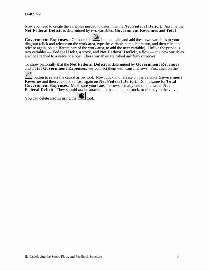
Now you need to create the variables needed to determine the Net Federal Deficit. Assume theNet Federal Deficit is determined by two variables, Government Revenues and Total

Government Expenses. Click on the button again and add these two variables to yourdiagram (click and release on the work area, type the variable name, hit return, and then click andrelease again, on a different part of the work area, to add the next variable). Unlike the previoustwo variables — Federal Debt, a stock, and Net Federal Deficit, a flow — the new variablesare not attached to a valve or a box. These variables are called auxiliary variables.

To show pictorially that the Net Federal Deficit is determined by Government Revenuesand Total Government Expenses, we connect them with causal arrows. First click on the

button to select the causal arrow tool. Now, click and release on the variable GovernmentRevenue and then click and release again on Net Federal Deficit. Do the same for TotalGovernment Expenses. Make sure your causal arrows actually end on the words NetFederal Deficit. They should not be attached to the cloud, the stock, or directly to the valve.

You can delete arrows using the tool.

D-4697-2


Clicking on the button allows you to select the variables you have created and move them todifferent places on the screen. To move variables, place the arrow cursor over the variable youwish to move, hold down the mouse button, move the variable to the desired place, and thenrelease the mouse button. You can also select the “handles” of the causal arrows (the small circlesin the middle of the arrow) and change the curvature of the arrow. Arrange your variables andarrows so that your diagram looks approximately like this:

Now, you may want to update your diagram by labeling the arrows to show that GovernmentRevenue and Total Government Expense affect the Net Federal Deficit in differentways. Specifically, an increase in revenue causes the deficit to decrease, while an increase in

expenses causes the deficit to increase. To do this, first click on the button. Then select the“handle” of the arrow you wish to label by clicking and releasing on the small circle in the middleof the arrow (the handle darkens when selected). Now, with the handle selected, click and release

the button on the bottom horizontal toolbar. You then see a pop-up menu that looks like this:

D-4697-2


Click and release on the desired label, and it will show up in the diagram. Label your two causalarrows so your diagram looks like this:

Now, using the same steps discussed above, complete the stock, flow and feedback so yourdiagram looks like this:

You may want to slide the handle of each arrow close to its arrowhead, so each label is clearlyassociated with its causal arrow.

D-4697-2


Finally, you may wish to label the positive feedback loop you have just created. Click on the button and then click in the center of the feedback loop. You can use this tool to create commentsthat, while having no structural use, can greatly help someone else to understand your modeldiagram. After clicking in the center of the loop, you should see the following dialog box:

Click on the Loop Clkwse button in the Shape box; click on Center in the Text Position box;and type R , for reinforcing, in the Comment box. You may also type + or P to denote a positivefeedback, also known as a reinforcing, loop. Your screen should now look like this:

D-4697-2


Click on the OK button or hit return.

Your screen should now appear as:

D-4697-2

III. Specifying Equations for Your Model 13

III. Specifying Equations for Your Model

Now that you have developed a complete stock, flow, and feedback representation of the deficit,you need to write equations for each of the variables. Equation formulation is a critical step in theprocess of model building and is a key part of the process of developing a rigorous understandingof the problem at hand.

To begin writing equations, click on the button on the sketch tool bar. The variables in yourdiagram become highlighted.

A highlighted variable indicates that the equation for that variable is incomplete.

Variables in system dynamics models are classified as either exogenous or endogenous.Exogenous variables are those that are not part of a feedback loop, while endogenous variables aremembers of at least one feedback loop. Your deficit model has three exogenous variables—Government Revenue, Other Government Expenses, and the Interest Rate—and fourendogenous variables—Interest Payments, Total Government Expense, Net FederalDeficit, and the Federal Debt.

D-4697-2


Start by writing the equations for the exogenous variables. To begin, click on the highlightedvariable Government Revenue. You then see the following dialog box:

Good modeling practice requires that each equation in a model have three elements: the equationitself, specified units of measure, and complete documentation. You enter the equation in the boxto the right of the = sign. You enter the unit of measure in the text field to the right of the wordUnits. Equation documentation or “comment” is entered in the box to the right of the wordComment.

To write an equation for Government Revenue, click in the box to the right of the = sign. Assumethat government revenue is constant, so that all you need to do is enter the appropriate number forgovernment revenue. In 1988, government revenue was about 900 billion dollars annually, sotype 900000000000 in the box. Alternatively, you can write 9e11, which is Vensim PLEshorthand for 9 * 1011 .

Now, fill in the units. Revenue is a flow variable, so the appropriate unit of measure for thisequation is dollars/time unit. Because you already chose to run the model in time steps of 1 year,the appropriate unit is dollars/year. Type dollars/year in the units field. (The next time youspecify the units for a variable in this model, dollars/year will appear in the units pull-down menu.You can click on the arrowhead to the right of the units field to see units already specified for othervariables in the model, and then use the mouse to select the units from that list when appropriate.)

Finally, provide a description of this equation in the comment field. A good comment will bebrief, but it will also give the reader the logic behind the equation as well as state the keyassumptions. For example, one might write for this equation:

Government revenues are assumed to be constant and equal to 900 billiondollars annually based on the actual value in 1988.

D-4697-2


Your dialog box should now look like this:

D-4697-2


Click on OK or hit return and your diagram will look like this:

Government Revenue is no longer highlighted because you have just specified its equation.

Following the process above, write equations for the two other exogenous variables, InterestRate and Other Government Expenses. Use the following information:

• Government expenses, excluding interest on the debt, were approximately 900 billiondollars in 1988.

• The interest rate paid on the national debt in 1988 was around 7%/year.

Now that the equations for the exogenous variables are formulated, turn your attention to theendogenous variables. Writing equations for the stocks and the flows is a little different, so let’sdo an example of each. First we formulate the equation for the stock, Federal Debt.

Again, click on the button on the sketch tool bar and then click on the stock, Federal Debt.

D-4697-2


The following dialog box will be displayed:

Unlike flows and constants, a stock requires that an additional element be specified in itsformulation; after you specify the equation, you need to select an initial or starting value.

You enter the equation for the stock in the box to the right of the word Integ. Integ stands for“integrate” and simply means that the stock at any moment in time is equal to the sum of all theinflows minus the sum of all the outflows plus the initial value.

When you created the stock, flow, and feedback diagram, you connected the flow Net FederalDeficit to the stock Federal Debt. Vensim PLE captures this stock-flow dependency byproviding a list of the required Variables to the stock Federal Debt on the right side of theequation dialog box. (The variable we are formulating, Federal Debt, itself also appears in theVariables box, but we focus on the input Net Federal Deficit. In general, you will neverwant to have the same variable on both the left and right sides of an equation.)

Because the model diagram shows the flow Net Federal Deficit feeding into the stock FederalDebt, Vensim has anticipated that the flow is an input to the stock equation and has placed the NetFederal Deficit variable name in the box to the right of Integ. If this is not the case in yourversion of Vensim PLE, then simply click in the box to the right of the Integ and then click on thevariable Net Federal Deficit in the Variables box to write the equation for the change inFederal Debt. (Note: If Net Federal Deficit is not in the Variables box, then your modeldiagram is incorrect and needs to be changed—make sure the flow is attached to the stock).

The Integ box should now look like this:

D-4697-2


Below the Integ box is the Initial Value box. Here you enter the initial condition or starting pointfor the stock. In 1988, the outstanding federal debt was approximately 2.5 trillion dollars, so enter2500000000000 in the initial value box (alternatively you can write 2.5e12, which is Vensim PLEshorthand for 2.5 x 1012). The Initial Value box should look like this:

Now the equation specification for the Federal Debt stock is complete. Your equation indicatesthat the federal debt is simply the accumulation of the Net Federal Deficit since 1988 added tothe initial value.

You still need to specify the unit of measure and document your equation in the comment field.The units should be fairly straightforward. The Federal Debt is a stock and its units are dollars.Useful comments briefly explain the structure of the equation and highlight the key assumptionsmade. A sample comment for Federal Debt is:

The Federal Debt is the accumulation of the Net Federal Deficit plus theinitial value of the debt. The initial value is set to 2.5 trillion dollars,which was the approximate outstanding federal debt in 1988—the startingpoint for this simulation.

D-4697-2


Your dialog box should now look like this:

D-4697-2


Click on OK or press return.

Now you need to specify the equations for the auxiliary variables and the flow.

Using the tool on the sketch tool bar, click on the Interest Payments variable. You shouldsee a dialog box that looks like this:

This box is identical to those used to specify the exogenous variables, but, in this case, there aretwo other variables in the Variables box; you are required to use these variables in the equation.When you developed the stock, flow, and feedback diagram, you drew causal arrows connectingthe variable Federal Debt and constant Interest Rate to the variable Interest Payments.Vensim PLE has conveniently recognized this fact and has provided a list of the required inputs toyour equation based on the picture you have already created. In fact, if you try to write yourequation without using the two required variables, Vensim PLE will give you an error message.

The rate of interest payment is simply equal to the current debt stock multiplied by the interest rate.To enter this equation, first click on the Federal Debt variable in the Variables box. It now

appears in the equation box. Now type * (alternatively you can click on the button), and thenclick on the Interest Rate variable in the Variables box. Your equation box should now looklike this:

D-4697-2


To complete the equation, you need to specify the units, dollars/year, and document your equationin the comment field. An appropriate comment might look like the following:

The annual flow of interest payments is equal to the current outstandingfederal debt multiplied by the annual interest rate.

The dialog box for the variable Interest Payments should now look like this:

Following a similar process to the one outlined above, you should now be able to complete yourmodel.

D-4697-2

IV. Using the Model Structure Analysis Tools 22

IV. Using the Model Structure Analysis Tools

Vensim PLE provides five tools for analyzing and understanding the structure of your model.

By far the most important of these is the unit-checking tool.

An important feature of any system dynamics equation is dimensional consistency, which is just afancy way of saying that the units of measure must be the same on both the left and right sides ofthe equation. As an example, suppose you had chosen the units of the Federal Debt stock to bedollars and the units of the Interest Rate to be dollars/year. If so, then pressing the apple keyand u (alternatively, you could select the Model menu, then select Units Check) simultaneouslywould yield the following message:

Followed by:

The problem is that, in this example, the equation for Interest Payments is not dimensionallyconsistent: the right and left sides of the equation have different units. The flow InterestPayments is measured in dollars per year. The Federal Debt, because it is a stock, is measured

D-4697-2


in dollars. Multiplying Federal Debt by something with units in dollars/year results in a quantitythat has units in dollars2/year—hence the error.

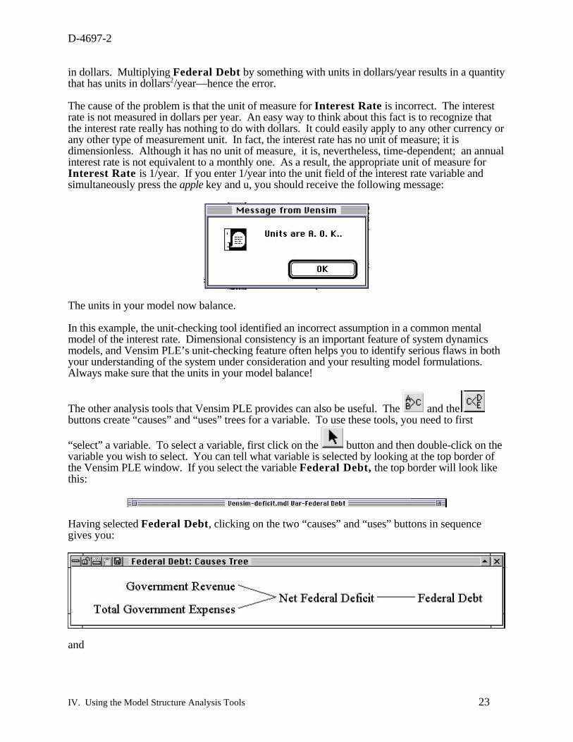
The cause of the problem is that the unit of measure for Interest Rate is incorrect. The interestrate is not measured in dollars per year. An easy way to think about this fact is to recognize thatthe interest rate really has nothing to do with dollars. It could easily apply to any other currency orany other type of measurement unit. In fact, the interest rate has no unit of measure; it isdimensionless. Although it has no unit of measure, it is, nevertheless, time-dependent; an annualinterest rate is not equivalent to a monthly one. As a result, the appropriate unit of measure forInterest Rate is 1/year. If you enter 1/year into the unit field of the interest rate variable andsimultaneously press the apple key and u, you should receive the following message:

The units in your model now balance.

In this example, the unit-checking tool identified an incorrect assumption in a common mentalmodel of the interest rate. Dimensional consistency is an important feature of system dynamicsmodels, and Vensim PLE’s unit-checking feature often helps you to identify serious flaws in bothyour understanding of the system under consideration and your resulting model formulations.Always make sure that the units in your model balance!

The other analysis tools that Vensim PLE provides can also be useful. The and the buttons create “causes” and “uses” trees for a variable. To use these tools, you need to first

“select” a variable. To select a variable, first click on the button and then double-click on thevariable you wish to select. You can tell what variable is selected by looking at the top border ofthe Vensim PLE window. If you select the variable Federal Debt, the top border will look likethis:

Having selected Federal Debt, clicking on the two “causes” and “uses” buttons in sequencegives you:

and

D-4697-2


The button on the analysis tool bar provides you with a complete listing of the equations in

your model. The tool on the analysis tool bar identifies all the feedback loops of which theselected variable is a member.

D-4697-2

V. Simulating Your Model 25

V. Simulating Your Model

Vensim PLE also has tools to help you analyze the behavior of your model. Before analyzing thebehavior, however, you must actually simulate the model so that you have some behavior toanalyze.

To run a simulation, you first need to click on the running man icon on the top toolbar.Vensim may display the following dialog box.

Clicking on yes will overwrite the “current” dataset displayed in the box to the right of the runningman icon. Selecting “No” will allow you to create a different dataset. It is helpful to choose namesthat suggest some idea of what is being tested rather than simply using name like SIM1, SIM2, etc.Because this run is the base case run for your model, you might choose to call the run BASE.*

Click on No, type in BASE as your new dataset name, click on Save or hit return, and your modelwill start simulating.

Once the simulation run is completed, you can look at the results of your simulation. Vensim PLEprovides many tools with which to view simulation output. The most basic, and often the mostuseful, of these tools is the strip graph. To create a graph of the Federal Debt, first click on the

tool and then double-click on the stock to select the variable Federal Debt.

To see a strip graph, click on the button on the analysis tool bar.

* Advanced Tip: Vensim PLE also offers you the choice of two numerical integration methods, Euler and Runge-Kutta 4.

Runge-Kutta 4 is a more accurate integration method, but it is also more computationally intensive. Generally it isbetter to use the Euler method and only change if you believe you are seeing integration error.

D-4697-2


You then see:

By the year 2010, given the current assumptions in the model, the federal debt will grow to morethan 10 trillion dollars, four times its value in 1988.

Besides the strip graph, Vensim PLE provides many other ways to examine simulation output.

The button displays a strip graph of the currently selected variable, along with graphs of allthe variables that determine the value of the selected variable (the causes). Clicking on the buttongives you:

D-4697-2


Vensim PLE also can present the output in the form of a table rather than a graph. To see a table of

the selected variable simply click on the button.

Having analyzed this simulation, you may wish to run additional simulations under differentassumptions. For example, what might happen if the prevailing interest rate were 3.5% rather than7%?

One way to change the parameter is to change the model equation in the original model. With the

button selected, click on Interest Rate. A dialog box will appear. In the constant boxchange the interest rate from 7% to 3.5%. Again, run this new simulation but do not overwrite thesimulation named Base. Instead, name it interest rate.

D-4697-2


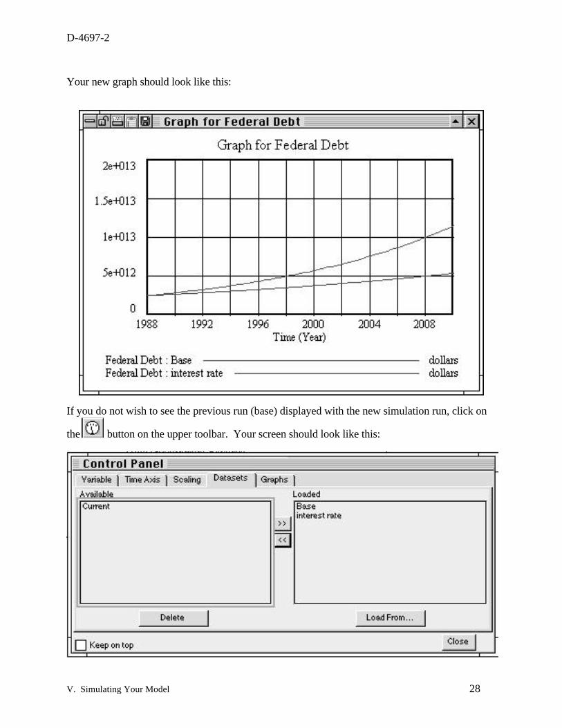
Your new graph should look like this:

If you do not wish to see the previous run (base) displayed with the new simulation run, click on

the button on the upper toolbar. Your screen should look like this:

D-4697-2


A dialog box appears and shows on the left side the two simulation runs you have created so far.Double-click on the name of the simulation run you wish to remove from the graph (or highlight itand click on the << button to remove it from the right side of the dialog box). Close the Datasetswindow and close and re-display the strip graph. Now, only the new simulation run shouldappear.

You may also wish to run the model for a longer period of time. In this case, select TimeBounds... from the Model menu. You then see the same dialog box that you saw when you firststarted to develop your model.

You can extend your simulation by setting a new date for your final time. Run your model out tothe year 2075.

Documents

Formulating Models of Simple Systems