Embed Size (px)
Citation preview

Formulating, Estimating, and Solving
Dynamic Equilibrium Models:
an Introduction
Jesus Fernandez-VillaverdeUniversity of Pennsylvania
1

Models
• Tradition in macroeconomics of using models:
1. Policy Analysis.
2. Forecasting.
3. Counterfactuals.
• This course reviews the recent advances in macroeconometric model-building.
2

Why Models?
• Organize our thinking.
• Reproducibility.
• Accumulation of capital within organizations.
• Ex-ante versus ex-post analysis.
• Counterfactuals.
• New circumstances.3

A Brief History of Macroeconometric Models: A Promising Beginning
• Old idea of economists: Quesnay, Walras.
• Pioneers: Tinbergen (1939, Noble Prize 1969), Haavelmo (1943, No-ble Prize 1989).
• Klein-Goldberger model (1955).
• Big models of the 1960s: Brookings, MIT-FRB-Penn, Wharton.
4

A Brief History of Macroeconometric Models: Disappointment
• 1970s and 1980s were the decades of disappointment
• Problems:
1. Fit (Nelson, 1972).
2. Nonstationarity (Granger, 1981).
3. Economic Foundations (Lucas, 1972).
5
A Brief History of Macroeconometric Models: Renewed Hopes
• 1980s: Real Business Cycle theory: advances and difficulties.
• Late 1990s, early 2000s: revival.
• Why?
1. Advances in economic theory: second generation equilibrium mod-
els.
2. Advances in econometrics: simulation methods.
6
Why Dynamic Equilibrium Models?
• Explicit microeconomic foundation.
• Robust to Lucas critique.
• Welfare analysis.
• Design of optimal policy.
7
A Brief History of Macroeconometric Models: References
• R.G. Bodking, L.R. Klein, and K. Marwah: A History of Macroecono-metric Model-Building, Edward Elgar, 1991.
• T.J. Sargent: Expectations and the Nonneutrality of Lucas, Journalof Monetary Economics, 1996.
8

Why Monetary Models?
• Is price stability a good idea? If so, at what price?
• How do we implement monetary policy?
• Does monetary policy have a role in stock market booms/busts?
• What do we in the wake of a monetary crisis?
• Why did inflation take off during the 1970s?
• Was the Great Depression caused by bad monetary policy?9

Is Money Important?
• At a basic level yes.
• “Lenin is said to have declared that the best way to destroy the Capi-talist System was to debauch its currency... Lenin was certainly right”.
J.M. Keynes (1919), The Economic Consequences of the Peace.
• Experiences of hyperinflation.
10

Money and the Business Cycle
• At a more moderate level, the question is surprisingly difficult to an-swer.
• Two “observations”:
1. Relation between Output and Money growth.
2. Phillips Curve.
• Where do these observations come?
11

“Conventional Wisdom”
• Old tradition in economics: Hume, Of Money, 1752.
• Friedman and Schwartz, A Monetary History of the US, 1963.
• Volcker’s recessions.
• Evidence from Structural Vector Autoregressions.
12

Structural Vector Autoregression
• SVARs have become a common tool among economists.
• Introduced by Sims (1980)
• SVARs make explicit identifying assumptions to isolate estimates ofpolicy and/or private agents behavior and its effects on the economy,
while keeping the model free of the many additional restrictive as-
sumptions needed to give every parameter a behavioral interpretation.
13

Uses of SVARs
1. The effects of money on output (Sims and Zha, 2005).
2. The relative importance of supply and demand shocks on output (Blan-
chard and Quah, 1989),
3. The effects of fiscal policy (Rotemberg and Woodford, 1992).
4. The relation between technology shocks and hours (Galı, 1999).
14

Economic Theory and the SVAR Representation
• Dynamic economic models can be viewed as restrictions on stochasticprocesses.
• An economic theory is a mapping between a vector of k economicshocks wt and a vector of n observables yt of the form
yt = D³wt´
• Interpretation.
15

Mapping
• The mapping D (·) is the product of the equilibrium behavior of the
agents in the model, implied by their optimal decision rules and the
consistency conditions like resource constraints and market clearing.
• The construction of the mapping D (·) is the sense in which economictheory tightly relates shocks and observables.
• The mapping D (·) can be interpreted as the impulse response of themodel to an economic shock.
16

A Linear Mapping
• We restrict our attention to linear mappings of the form:yt = D (L)wt
where L is the lag operator.
• wt ∼ N (0,Σ) .
• More involved structures?
17
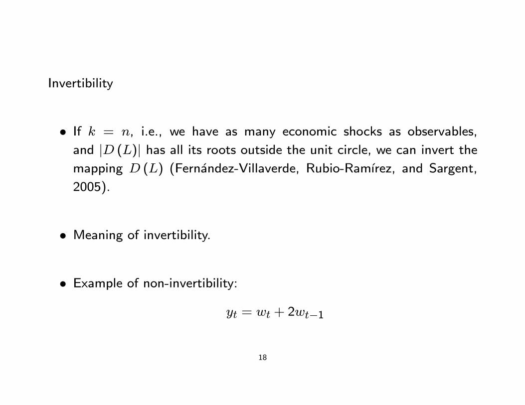
Invertibility
• If k = n, i.e., we have as many economic shocks as observables,
and |D (L)| has all its roots outside the unit circle, we can invert themapping D (L) (Fernandez-Villaverde, Rubio-Ramırez, and Sargent,
2005).
• Meaning of invertibility.
• Example of non-invertibility:yt = wt + 2wt−1
18
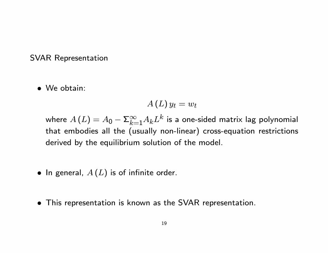
SVAR Representation
• We obtain:A (L) yt = wt
where A (L) = A0 −Σ∞k=1AkLk is a one-sided matrix lag polynomialthat embodies all the (usually non-linear) cross-equation restrictions
derived by the equilibrium solution of the model.
• In general, A (L) is of infinite order.
• This representation is known as the SVAR representation.
19

Reduced Form Representation
• Consider now the case where a researcher does not have access to theSVAR representation. Instead, she has access to the VAR representa-
tion of yt:
yt = B1yt−1 +B2yt−2 + ...+ at,
where Eyt−jat = 0 for all j and Eata0t = Ω.
• This representation is known as the Reduced form representation.
• Can the researcher recover the SVAR representation using the Reducedform representation?
20
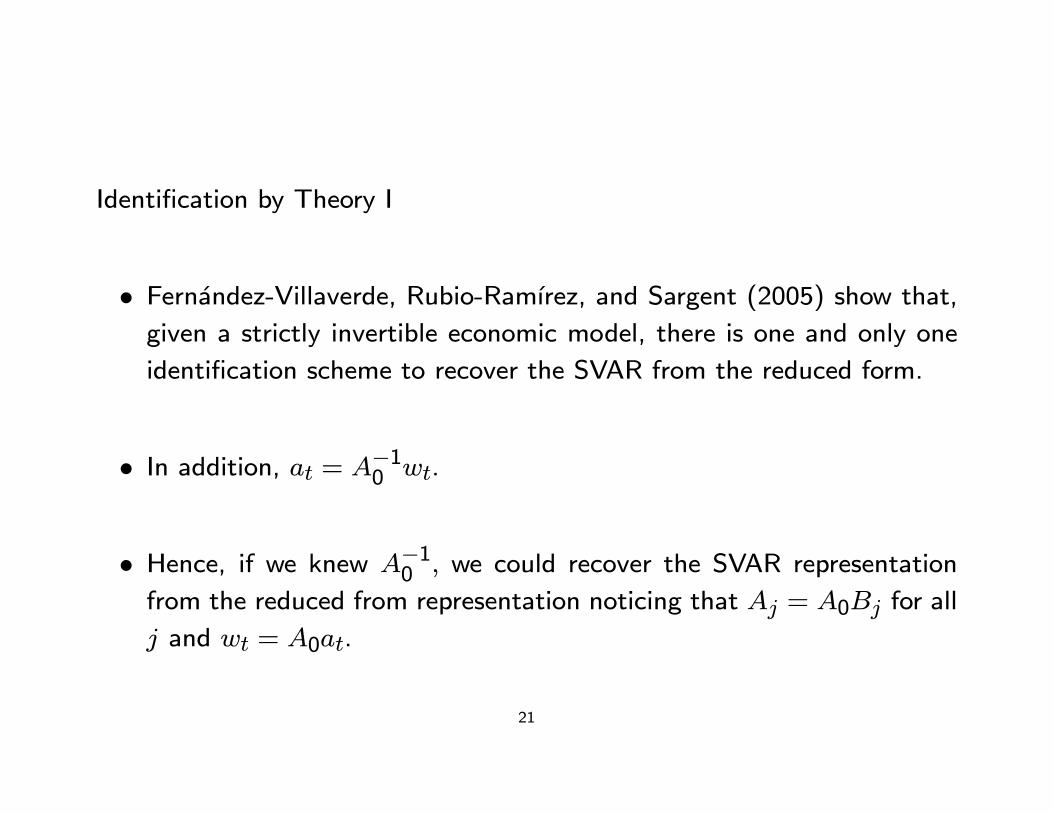
Identification by Theory I
• Fernandez-Villaverde, Rubio-Ramırez, and Sargent (2005) show that,given a strictly invertible economic model, there is one and only one
identification scheme to recover the SVAR from the reduced form.
• In addition, at = A−10 wt.
• Hence, if we knew A−10 , we could recover the SVAR representation
from the reduced from representation noticing that Aj = A0Bj for all
j and wt = A0at.
21

Identification by Theory II
• Fernandez-Villaverde, Rubio-Ramırez, and Sargent’s identification re-quires the specification of an explicit dynamic economic model.
• Can we avoid this step? Unfortunately, the answer is in general no,
because knowledge of the reduced form matrices Bi’s and Ω does not
imply, by itself, knowledge of the Ai’s and Σ.
• Why: normalization and identification.
22

Normalization
• Reversing the signs of two rows or columns of the Ai’s does not matterfor the Bi’s.
• Thus, without the correct normalization restrictions, statistical infer-ence about the Ai’s is essentially meaningless.
• Waggoner and Zha (2003) provide a general normalization rule thatmaintains coherent economic interpretations.
23

Identification I
• If we knew A0, each equation Bi = A−10 Ai would determine Ai given
some Bi.
• But in Ω = A0ΣA00 we n (3n+ 1) /2 unknowns (the n
2 distinct ele-
ments of A0 and the n (n+ 1) /2 distinct elements of Σ) for n2 knows
(the n (n+ 1) /2 distinct elements of Ω).
• Thus, we require n2 identification restrictions.
24

Identification II
• Since can set the diagonal elements of A0 equal to 1 by scaling, we areleft with the need of n (n− 1) additional identification restrictions.
• Alternatively, we could scale the shocks such that the diagonal of Σis composed of ones and leave the diagonal of A0 unrestricted.
• These identification restrictions are dictated by the economic theorybeing studied.
25

Identification III
• What about identification restrictions compatible with a large class ofmodels?
• Robustness versus efficiency.
• Discussion of trade-off.
26

Identification IV
• Most common identification restrictions: Σ is diagonal.
• Why?
• Since this assumption imposes n (n− 1) /2 restrictions, we still requiren (n− 1) /2 additional restrictions.
27
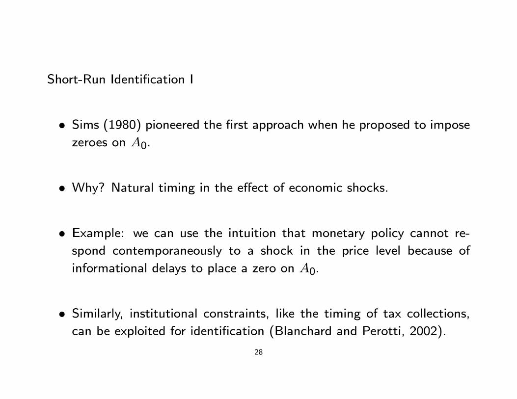
Short-Run Identification I
• Sims (1980) pioneered the first approach when he proposed to imposezeroes on A0.
• Why? Natural timing in the effect of economic shocks.
• Example: we can use the intuition that monetary policy cannot re-spond contemporaneously to a shock in the price level because of
informational delays to place a zero on A0.
• Similarly, institutional constraints, like the timing of tax collections,can be exploited for identification (Blanchard and Perotti, 2002).
28

Short-Run Identification II
• Sims (1980) ordered variables in such a way that A0 is lower triangular.
• Sims and Zha (2005) present a non-triangular, identification schemeon an eight-variable SVAR.
• We will come back to Sims and Zha (2005).
29

Long-Run Identification I
• Blanchard and Quah (1989).
• Restriction imposed on A (1) = A0 − Σ∞k=1Ak.
• Since A−1 (1) = D (1), long-run restrictions are restrictions on the
long-run effects of economic shocks, usually on the first difference of
an observable.
30

Long-Run Identification II
• Blanchard and Quah (1989): demand shock has no effect long-runeffect on unemployment or output while supply shock has no long-run
on unemployment, but may have a long-run effect on output.
• Galı (1999): technology shocks has no effect long-run effect on hoursand but it has on productivity.
31
New Identification Schemes
• Uhlig (2005): sign restrictions. Identifies a contractionary monetarypolicy shock as one that does not lead to an increase in prices or in
nonborrowed reserves and does not lead to a decrease in the federal
funds rate.
• Faust, Swanson, and Wright (2004) identify the effects if a monetaryshock in a SVAR using the prices of federal funds futures contracts.
32

Estimable Equation
• Why is the previous discussion of the relation between the reducedand structural form of a VAR relevant?
• Because the reduced form can be easily estimated.
• An empirically implementable version of the reduced form representa-
tion truncates the number of lags at the p-th order:
yt = B∗1yt−1 + ...+B∗pyt−p + a∗t
where Ea∗t a∗0t = Ω∗.
33

Effects of Truncation
• Bad: Chari, Kehoe, McGrattan (2005).
• Not too bad: Christiano, Eichenbaum, and Vigfusson (2005).
• Problems with infinite dimensional estimation: Faust and Leeper,
1997).
34

Estimation
• Classical: GMM, ML, OLS.
• Bayesian.
• Why Bayesian? Overparametrization and priors.
• We will talk about these issues later.
35

Estimation
• Point estimates B∗i for i = 1, .., p and Ω∗
• Then, we find estimates of Ai and Σ by solving B∗i = A−1i Ai for
i = 1, ..., p, and Ω∗ = A0ΣA00.
• Finally, wt = A0a∗t .
36

An Example: Sims and Zha (2005)
• A simple, model-based SVAR.
• U.S. Quarterly Data 1964-1994.
• 8 variables.
• We will need at least (8 ∗ 7) /2 = 28 identification restrictions.
37

Variables
R: federal funds rate.M : M2.Py: GNP deflator.y: real GNP.W : average hourly earnings of non-agricultural workers.Pim: producers’ price index.Tbk: bankruptcy filings, personal and business.Pcm: producer’ price index for intermediate goods.
38
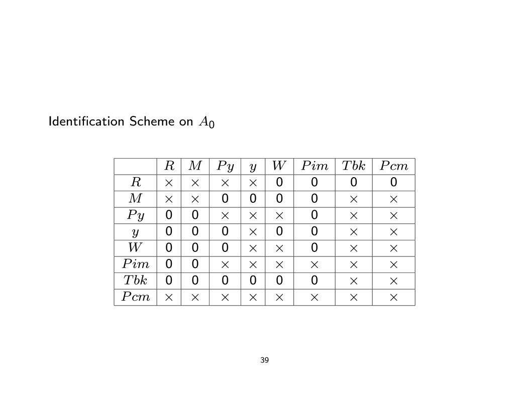
Identification Scheme on A0
R M Py y W Pim Tbk PcmR × × × × 0 0 0 0M × × 0 0 0 0 × ×Py 0 0 × × × 0 × ×y 0 0 0 × 0 0 × ×W 0 0 0 × × 0 × ×Pim 0 0 × × × × × ×Tbk 0 0 0 0 0 0 × ×Pcm × × × × × × × ×
39
Comments on Identification
• Sims and Zha impose exactly 28 identification restrictions.
• Motivated by an economic model.
• Intuition guides the choice of model.
40

Figure 2Impulse Reponses: M2 Model
Res
pons
e of
Pcm (309e-4)
M (771e-5)
R (566e-5)
Pim (173e-4)
Py (432e-5)
W (499e-5)
y (715e-5)
Tbk (356e-4)
Pcm MD MS Pim Py W y Tbk

Figure 4aM Decomposition, M2 Model
Forecast Errors1965 1967 1969 1971 1973 1975 1977 1979 1981 1983 1985 1987 1989 1991 1993
-0.064-0.048-0.032-0.0160.0000.0160.0320.0480.064
PCM1965 1967 1969 1971 1973 1975 1977 1979 1981 1983 1985 1987 1989 1991 1993
-0.064-0.048-0.032-0.0160.0000.0160.0320.0480.064
MD1965 1967 1969 1971 1973 1975 1977 1979 1981 1983 1985 1987 1989 1991 1993
-0.064-0.048-0.032-0.0160.0000.0160.0320.0480.064

Figure 4bM Decomposition, M2 Model
MS1965 1967 1969 1971 1973 1975 1977 1979 1981 1983 1985 1987 1989 1991 1993
-0.064-0.048-0.032-0.0160.0000.0160.0320.0480.064
PIM1965 1967 1969 1971 1973 1975 1977 1979 1981 1983 1985 1987 1989 1991 1993
-0.064-0.048-0.032-0.0160.0000.0160.0320.0480.064
PY1965 1967 1969 1971 1973 1975 1977 1979 1981 1983 1985 1987 1989 1991 1993
-0.064-0.048-0.032-0.0160.0000.0160.0320.0480.064

Figure 4cM Decomposition, M2 Model
W1965 1967 1969 1971 1973 1975 1977 1979 1981 1983 1985 1987 1989 1991 1993
-0.064-0.048-0.032-0.0160.0000.0160.0320.0480.064
Y1965 1967 1969 1971 1973 1975 1977 1979 1981 1983 1985 1987 1989 1991 1993
-0.064-0.048-0.032-0.0160.0000.0160.0320.0480.064
TBK1965 1967 1969 1971 1973 1975 1977 1979 1981 1983 1985 1987 1989 1991 1993
-0.064-0.048-0.032-0.0160.0000.0160.0320.0480.064

Figure 5aR Decomposition, M2 Model
Forecast Errors1965 1967 1969 1971 1973 1975 1977 1979 1981 1983 1985 1987 1989 1991 1993
-0.04
-0.02
0.00
0.02
0.04
0.06
0.08
PCM1965 1967 1969 1971 1973 1975 1977 1979 1981 1983 1985 1987 1989 1991 1993
-0.04
-0.02
0.00
0.02
0.04
0.06
0.08
MD1965 1967 1969 1971 1973 1975 1977 1979 1981 1983 1985 1987 1989 1991 1993
-0.04
-0.02
0.00
0.02
0.04
0.06
0.08
Figure 5bR Decomposition, M2 Model
MS1965 1967 1969 1971 1973 1975 1977 1979 1981 1983 1985 1987 1989 1991 1993
-0.04
-0.02
0.00
0.02
0.04
0.06
0.08
PIM1965 1967 1969 1971 1973 1975 1977 1979 1981 1983 1985 1987 1989 1991 1993
-0.04
-0.02
0.00
0.02
0.04
0.06
0.08
PY1965 1967 1969 1971 1973 1975 1977 1979 1981 1983 1985 1987 1989 1991 1993
-0.04
-0.02
0.00
0.02
0.04
0.06
0.08

Figure 5cR Decomposition, M2 Model
W1965 1967 1969 1971 1973 1975 1977 1979 1981 1983 1985 1987 1989 1991 1993
-0.04
-0.02
0.00
0.02
0.04
0.06
0.08
Y1965 1967 1969 1971 1973 1975 1977 1979 1981 1983 1985 1987 1989 1991 1993
-0.04
-0.02
0.00
0.02
0.04
0.06
0.08
TBK1965 1967 1969 1971 1973 1975 1977 1979 1981 1983 1985 1987 1989 1991 1993
-0.04
-0.02
0.00
0.02
0.04
0.06
0.08

Figure 6aPy Decomposition, M2 Model
Forecast Errors1965 1967 1969 1971 1973 1975 1977 1979 1981 1983 1985 1987 1989 1991 1993
-0.04
-0.02
0.00
0.02
0.04
0.06
PCM1965 1967 1969 1971 1973 1975 1977 1979 1981 1983 1985 1987 1989 1991 1993
-0.04
-0.02
0.00
0.02
0.04
0.06
MD1965 1967 1969 1971 1973 1975 1977 1979 1981 1983 1985 1987 1989 1991 1993
-0.04
-0.02
0.00
0.02
0.04
0.06
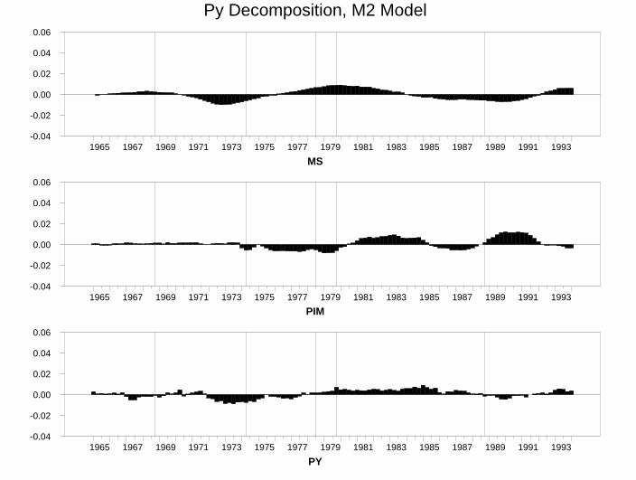
Figure 6bPy Decomposition, M2 Model
MS1965 1967 1969 1971 1973 1975 1977 1979 1981 1983 1985 1987 1989 1991 1993
-0.04
-0.02
0.00
0.02
0.04
0.06
PIM1965 1967 1969 1971 1973 1975 1977 1979 1981 1983 1985 1987 1989 1991 1993
-0.04
-0.02
0.00
0.02
0.04
0.06
PY1965 1967 1969 1971 1973 1975 1977 1979 1981 1983 1985 1987 1989 1991 1993
-0.04
-0.02
0.00
0.02
0.04
0.06
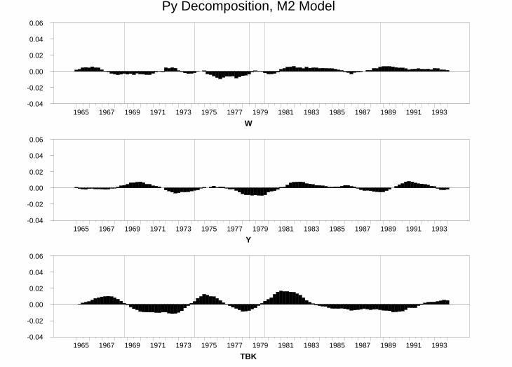
Figure 6cPy Decomposition, M2 Model
W1965 1967 1969 1971 1973 1975 1977 1979 1981 1983 1985 1987 1989 1991 1993
-0.04
-0.02
0.00
0.02
0.04
0.06
Y1965 1967 1969 1971 1973 1975 1977 1979 1981 1983 1985 1987 1989 1991 1993
-0.04
-0.02
0.00
0.02
0.04
0.06
TBK1965 1967 1969 1971 1973 1975 1977 1979 1981 1983 1985 1987 1989 1991 1993
-0.04
-0.02
0.00
0.02
0.04
0.06

Figure 7ay Decomposition, M2 Model
Forecast Errors1965 1967 1969 1971 1973 1975 1977 1979 1981 1983 1985 1987 1989 1991 1993
-0.064-0.048-0.032-0.0160.0000.0160.0320.0480.064
PCM1965 1967 1969 1971 1973 1975 1977 1979 1981 1983 1985 1987 1989 1991 1993
-0.064-0.048-0.032-0.0160.0000.0160.0320.0480.064
MD1965 1967 1969 1971 1973 1975 1977 1979 1981 1983 1985 1987 1989 1991 1993
-0.064-0.048-0.032-0.0160.0000.0160.0320.0480.064

Figure 7by Decomposition, M2 Model
MS1965 1967 1969 1971 1973 1975 1977 1979 1981 1983 1985 1987 1989 1991 1993
-0.064-0.048-0.032-0.0160.0000.0160.0320.0480.064
PIM1965 1967 1969 1971 1973 1975 1977 1979 1981 1983 1985 1987 1989 1991 1993
-0.064-0.048-0.032-0.0160.0000.0160.0320.0480.064
PY1965 1967 1969 1971 1973 1975 1977 1979 1981 1983 1985 1987 1989 1991 1993
-0.064-0.048-0.032-0.0160.0000.0160.0320.0480.064

Figure 7cy Decomposition, M2 Model
W1965 1967 1969 1971 1973 1975 1977 1979 1981 1983 1985 1987 1989 1991 1993
-0.064-0.048-0.032-0.0160.0000.0160.0320.0480.064
Y1965 1967 1969 1971 1973 1975 1977 1979 1981 1983 1985 1987 1989 1991 1993
-0.064-0.048-0.032-0.0160.0000.0160.0320.0480.064
TBK1965 1967 1969 1971 1973 1975 1977 1979 1981 1983 1985 1987 1989 1991 1993
-0.064-0.048-0.032-0.0160.0000.0160.0320.0480.064

Figure 8aTime Series of Structural Disturbances: M2 Model
Pcm1965 1967 1969 1971 1973 1975 1977 1979 1981 1983 1985 1987 1989 1991 1993
-0.27-0.18-0.09-0.000.090.180.27
MD1965 1967 1969 1971 1973 1975 1977 1979 1981 1983 1985 1987 1989 1991 1993
-0.03-0.02-0.010.000.010.020.03
MS1965 1967 1969 1971 1973 1975 1977 1979 1981 1983 1985 1987 1989 1991 1993
-0.072-0.054-0.036-0.0180.0000.0180.0360.054
Pim1965 1967 1969 1971 1973 1975 1977 1979 1981 1983 1985 1987 1989 1991 1993
-0.030-0.025-0.020-0.015-0.010-0.0050.0000.0050.0100.015

Figure 8bTime Series of Structural Disturbances: M2 Model
W1965 1967 1969 1971 1973 1975 1977 1979 1981 1983 1985 1987 1989 1991 1993
-0.0100-0.0075-0.0050-0.00250.00000.00250.0050
Py1965 1967 1969 1971 1973 1975 1977 1979 1981 1983 1985 1987 1989 1991 1993
-0.006-0.004-0.0020.0000.0020.0040.0060.0080.010
y1965 1967 1969 1971 1973 1975 1977 1979 1981 1983 1985 1987 1989 1991 1993
-0.03-0.02-0.010.000.010.020.03
Tbk1965 1967 1969 1971 1973 1975 1977 1979 1981 1983 1985 1987 1989 1991 1993
-0.075-0.050-0.0250.0000.0250.0500.075

Figure 9Fixed R Policy: M2 Model
Res
pons
e of
Pcm (296e-4)
M (110-5)
R (558e-5)
Pim (160e-4)
Py (415e-5)
W (456e-5)
y (679e-5)
Tbk (237e-4)
Pcm MD MS Pim Py W y Tbk

Figure 10Fixed M Policy: M2 Model
Res
pons
e of
Pcm (278e-4)
M (700-5)
R (518e-5)
Pim (153e-4)
Py (364e-5)
W (373e-5)
y (577e-5)
Tbk (287e-4)
Pcm MS MD Pim Py W y Tbk

Assessment and Criticisms of SVARs
• SVARs offer an attractive approach to estimation.
• They promise to coax interesting patterns from the data that will
prevail across a set of incompletely specified dynamic economic model
with a minimum of identifying assumptions.
• Moreover, SVAR are easy to estimate.
• SVAR have contributed to the understanding of aggregate fluctuations,to clarify the importance of different economic shocks, and to generate
fruitful debates among macroeconomists.
41

Criticisms of SVARs I
• Economic shocks recovered from a SVAR do not resemble the shocksmeasured by other mechanisms, like market expectations (Rudebusch,1998).
• Shocks recovered from a SVAR may reflect variables omitted from themodel. If these omitted variables correlate with the included variables,the estimated economic shocks will be biased.
• Example→“price puzzle”: early SVARs found that inflation increasedafter a contractionary monetary policy shock.
• Sims (1992): the Fed looks forward when it sets the federal fund rate.Solution?
42

Criticisms of SVARs II
• Many SVAR exercises, even simple ones, are sensitive to the identifi-cation restrictions, Stock and Watson (2001).
• Many of the identification schemes are the product of an specificationsearch in which researchers look for “reasonable” answers. If an identi-
fication scheme matches the conventional wisdom is called successful,
if it does not is called a puzzle or, even worse, a failure (Uhlig, 2005).
43