P2. Formula Sheets

Bionic Turtle FRM Formula Sheets

By David Harper, CFA FRM CIPM www.bionicturtle.com

Note: If you are unable to view the content within this document we recommend the following: MAC Users: The built-in pdf reader will not display our non-standard fonts. Please use adobe’s pdf reader. PC Users: We recommend you use the foxit pdf reader or adobe’s pdf reader. Mobile and Tablet users: We recommend you use the foxit pdf reader app or the adobe pdf reader app. All of these products are free. We apologize for any inconvenience. If you have any additional problems, please email Suzanne.

2

HULL, CHAPTER 19: VOLATILITY SMILES: EXPLAIN HOW PUT-CALL PARITY INDICATES THAT THE IMPLIED

VOLATILITY USED TO PRICE CALL OPTIONS IS THE SAME USED TO PRICE PUT OPTIONS. ...................................... 6 CALCULATE THE EXPECTED DISCOUNTED VALUE OF A ZERO-COUPON SECURITY USING A BINOMIAL TREE. ........... 7 CONSTRUCT AND APPLY AN ARBITRAGE ARGUMENT TO PRICE A CALL OPTION ON A ZERO-COUPON SECURITY USING

REPLICATING PORTFOLIOS. ...................................................................................................................... 8 CALCULATE THE CONVEXITY EFFECT USING JENSEN’S INEQUALITY. ............................................................... 9 TUCKMAN, CHAPTER 9: THE ART OF TERM STRUCTURE MODELS: DRIFT. DESCRIBE THE PROCESS AND

EFFECTIVENESS OF THE FOLLOWING MODELS, AND CONSTRUCT TREE FOR A SHORT-TERM RATE USING THE

FOLLOWING MODELS: A MODEL WITH NORMALLY DISTRIBUTED RATES AND NO DRIFT (MODEL 1) ...................... 9 DESCRIBE … A MODEL INCORPORATING DRIFT (MODEL 2) ......................................................................... 10 CALCULATE THE SHORT-TERM RATE CHANGE AND STANDARD DEVIATION OF THE CHANGE OF THE RATE USING A

MODEL WITH NORMALLY DISTRIBUTED RATES [ASSUMING BOTH DRIFT] AND NO DRIFT. .................................. 11 DESCRIBE THE PROCESS OF AND CONSTRUCT A TREE FOR A SHORT-TERM RATE UNDER THE HO-LEE MODEL WITH

TIME DEPENDENT DRIFT. ....................................................................................................................... 12 DESCRIBE THE PROCESS OF AND CONSTRUCT A SIMPLE AND RECOMBINING TREE FOR A SHORT-TERM RATE UNDER

THE VASICEK MODEL WITH MEAN REVERSION. ......................................................................................... 12 CALCULATE THE VASICEK MODEL RATE CHANGE, STANDARD DEVIATION OF THE CHANGE OF THE RATE, EXPECTED

RATE IN T YEARS, AND HALF-LIFE. .......................................................................................................... 13 TUCKMAN, CHAPTER 10: THE ART OF TSM: VOLATILITY & DISTRIBUTION. DESCRIBE THE SHORT-TERM RATE

PROCESS UNDER A MODEL WITH TIME-DEPENDENT VOLATILITY (MODEL 3). ................................................. 14 CALCULATE THE SHORT-TERM RATE CHANGE AND DESCRIBE THE BEHAVIOR OF THE STANDARD DEVIATION OF THE

CHANGE OF THE RATE USING A MODEL WITH TIME DEPENDENT VOLATILITY. .................................................. 14 DESCRIBE THE SHORT-TERM RATE PROCESS UNDER THE COX-INGERSOLL-ROSS (CIR) AND LOGNORMAL

MODELS. ............................................................................................................................................. 15 DESCRIBE THE IMPACT ON A MBS OF THE WEIGHTED AVERAGE MATURITY, THE WEIGHTED AVERAGE COUPON, AND THE SPEED OF PREPAYMENTS OF THE MORTGAGES UNDERLYING THE MBS. ........................................... 16 IDENTIFY, DESCRIBE, AND CONTRAST DIFFERENT STANDARD PREPAYMENT MEASURES. .................................. 16 DESCRIBE THE EFFECTIVE DURATION AND EFFECTIVE CONVEXITY OF STANDARD MBS INSTRUMENTS AND THE

FACTORS THAT AFFECT THEM. ................................................................................................................ 18 DOWD, MEASURING, CHAPTER 3: ESTIMATING MARKET RISK MEASURES. CALCULATE VAR USING A HISTORICAL

SIMULATION APPROACH ........................................................................................................................ 18 CALCULATE VAR USING A PARAMETRIC ESTIMATION APPROACH ASSUMING THAT THE RETURN DISTRIBUTION IS

EITHER NORMAL OR LOGNORMAL. .......................................................................................................... 19 CALCULATE EXPECTED SHORTFALL GIVEN P/L OR RETURN DATA. ............................................................... 20 DEFINE COHERENT RISK MEASURES. ....................................................................................................... 20 DESCRIBE THE METHOD OF ESTIMATING COHERENT RISK MEASURES BY ESTIMATING QUANTILES. .................... 22 DESCRIBE THE FOLLOWING WEIGHTED HISTORIC SIMULATION APPROACHES: AGE-WEIGHTED HISTORIC

SIMULATION ........................................................................................................................................ 23 DESCRIBE THE FOLLOWING WEIGHTED HISTORIC SIMULATION APPROACHES: VOLATILITY-WEIGHTED HISTORIC

SIMULATION ........................................................................................................................................ 24 DOWD, CHAPTER 5 APPENDIX: MODELING DEPENDENCE: CORRELATIONS AND COPULAS. EXPLAIN THE

DRAWBACKS OF USING CORRELATION TO MEASURE DEPENDENCE. .............................................................. 25 DESCRIBE HOW COPULAS PROVIDE AN ALTERNATIVE MEASURE OF DEPENDENCE. ......................................... 25 IDENTIFY BASIC EXAMPLES OF COPULAS. ................................................................................................. 26 EXPLAIN HOW TAIL DEPENDENCE CAN BE INVESTIGATED USING COPULAS. ................................................... 27 DOWD, CHAPTER 7: PARAMETRIC APPROACHES (II): EXTREME VALUE. COMPARE GENERALIZED EXTREME VALUE

AND POT. DESCRIBE THE PARAMETERS OF A GENERALIZED PARETO (GP) DISTRIBUTION. ............................. 27

3

COMPUTE VAR AND EXPECTED SHORTFALL USING THE POT APPROACH, GIVEN VARIOUS PARAMETER VALUES. . 28 DESCRIBE AND CALCULATE THE MORTGAGE PAYMENT FACTOR. .................................................................. 29 CALCULATE THE STATIC CASH FLOW YIELD OF A MBS USING BOND EQUIVALENT YIELD (BEY) AND DETERMINE

THE ASSOCIATED NOMINAL SPREAD. ....................................................................................................... 29 DESCRIBE THE STEPS FOR VALUING A MORTGAGE SECURITY USING MONTE CARLO METHODOLOGY. ................. 31 DEFINE AND INTERPRET OPTION-ADJUSTED SPREAD (OAS), ZERO-VOLATILITY OAS, AND OPTION COST. .......... 33 EXPLAIN HOW TO SELECT THE NUMBER OF INTEREST RATE PATHS IN MONTE CARLO ANALYSIS. ....................... 34 DESCRIBE TOTAL RETURN ANALYSIS, CALCULATE TOTAL RETURN, AND UNDERSTAND FACTORS PRESENT IN MORE

SOPHISTICATED MODELS. ...................................................................................................................... 35 SERVIGNY, CHAPTER 3: DEFAULT RISK: QUANTITATIVE METHODOLOGIES. DESCRIBE THE MERTON MODEL FOR

CORPORATE SECURITY PRICING, INCLUDING ITS ASSUMPTIONS, STRENGTHS AND WEAKNESSES. ....................... 36 USING THE MERTON MODEL, CALCULATE THE VALUE OF A FIRM'S DEBT AND EQUITY AND THE VOLATILITY OF FIRM

VALUE. ............................................................................................................................................... 37 DEFINE THE FOLLOWING TERMS RELATED TO DEFAULT AND RECOVERY: DEFAULT EVENTS, PROBABILITY OF

DEFAULT, CREDIT EXPOSURE, AND LOSS GIVEN DEFAULT. .......................................................................... 42 CALCULATE EXPECTED LOSS FROM RECOVERY RATES, THE LOSS GIVEN DEFAULT, AND THE PROBABILITY OF

DEFAULT. ............................................................................................................................................ 44 DESCRIBE THE MERTON MODEL, AND USE IT TO CALCULATE THE VALUE OF A FIRM, THE VALUES OF A FIRM’S DEBT

AND EQUITY, AND DEFAULT PROBABILITIES. ............................................................................................. 45 DESCRIBE CREDIT FACTOR MODELS AND EVALUATE AN EXAMPLE OF A SINGLE-FACTOR MODEL. ...................... 47 DEFINE CREDIT VAR (VALUE-AT-RISK). .................................................................................................. 48 MALZ, CHAPTER 7: SPREAD RISK AND DEFAULT INTENSITY MODELS. DEFINE THE DIFFERENT WAYS OF

REPRESENTING SPREADS. COMPARE AND DIFFERENTIATE BETWEEN THE DIFFERENT SPREAD CONVENTIONS AND

COMPUTE ONE SPREAD GIVEN OTHERS WHEN POSSIBLE. ............................................................................ 50 EXPLAIN HOW DEFAULT RISK FOR A SINGLE COMPANY CAN BE MODELED AS A BERNOULLI TRIAL. .................... 51 DEFINE THE HAZARD RATE AND USE IT TO DEFINE PROBABILITY FUNCTIONS FOR DEFAULT TIME AND CONDITIONAL

DEFAULT PROBABILITIES. ...................................................................................................................... 51 CALCULATE RISK-NEUTRAL DEFAULT RATES FROM SPREADS. ..................................................................... 52 DEFINE DEFAULT CORRELATION FOR CREDIT PORTFOLIOS. ......................................................................... 53 DESCRIBE HOW A SINGLE FACTOR MODEL CAN BE USED TO MEASURE CONDITIONAL DEFAULT PROBABILITIES

GIVEN ECONOMIC HEALTH. .................................................................................................................... 53 COMPUTE VARIANCE OF THE CONDITIONAL DEFAULT DISTRIBUTION AND CONDITIONAL PROBABILITY OF DEFAULT

USING SINGLE-FACTOR MODEL. .............................................................................................................. 54 EXPLAIN HOW CREDIT VAR OF A PORTFOLIO IS CALCULATED USING THE SINGLE-FACTOR MODEL, AND HOW

CORRELATION AFFECTS THE DISTRIBUTION OF LOSS SEVERITY FOR INTERMEDIATE VALUES BETWEEN 0 AND 1. .. 55 GREGORY, CHAPTER 2: DEFINING COUNTERPARTY CREDIT RISK ................................................................ 55 DEFINE THE FOLLOWING METRICS FOR CREDIT EXPOSURE: EXPECTED MARK-TO-MARKET, EXPECTED EXPOSURE, POTENTIAL FUTURE EXPOSURE, EXPECTED POSITIVE EXPOSURE, EFFECTIVE EXPOSURE, AND MAXIMUM

EXPOSURE. ......................................................................................................................................... 56 DESCRIBE THE PARAMETERS USED IN SIMPLE SINGLE-FACTOR MODELS … .................................................... 58 DESCRIBE HOW NETTING IS MODELED. .................................................................................................... 60 DEFINE AND CALCULATE THE NETTING FACTOR......................................................................................... 61 DEFINE AND CALCULATE MARGINAL EXPECTED EXPOSURE AND THE EFFECT OF CORRELATION ON TOTAL

EXPOSURE. ......................................................................................................................................... 61 GREGORY, CHAPTER 5: QUANTIFYING COUNTERPARTY CREDIT EXPOSURE, II: THE IMPACT OF COLLATERAL. CALCULATE THE EXPECTED EXPOSURE AND POTENTIAL FUTURE EXPOSURE OVER THE REMARGINING PERIOD

GIVEN NORMAL DISTRIBUTION ASSUMPTIONS. .......................................................................................... 61

4

DEFINE AND CALCULATE CREDIT VALUE ADJUSTMENT (CVA) WHEN NO WRONG-WAY RISK IS PRESENT. ........... 62 DESCRIBE THE PROCESS OF APPROXIMATING THE CVA SPREAD. ................................................................. 63 DEFINE AND CALCULATE THE INCREMENTAL CVA AND THE MARGINAL CVA. ................................................ 63 DEFINE AND CALCULATE CVA AND CVA SPREAD IN THE PRESENCE OF A BILATERAL CONTRACT. ..................... 64 CROUHY CHAPTER 14: DESCRIBE RAROC (RISK-ADJUSTED RETURN ON CAPITAL) METHODOLOGY .................. 65 COMPUTE AND INTERPRET THE RAROC FOR A LOAN OR LOAN PORTFOLIO, AND USE RAROC TO COMPARE

BUSINESS UNIT PERFORMANCE. ............................................................................................................. 66 EXPLAIN HOW THE SECOND-GENERATION RAROC APPROACHES IMPROVE ECONOMIC CAPITAL ALLOCATION

DECISIONS .......................................................................................................................................... 67 COMPUTE THE ADJUSTED RAROC FOR A PROJECT TO DETERMINE ITS VIABILITY. ........................................... 68 DESCRIBE AND CALCULATE LVAR USING THE CONSTANT SPREAD APPROACH AND THE EXOGENOUS SPREAD

APPROACH. ......................................................................................................................................... 74 DESCRIBE ENDOGENOUS PRICE APPROACHES TO LVAR, ITS MOTIVATION AND LIMITATIONS. .......................... 75 CALCULATE A FIRM’S LEVERAGE RATIO, DESCRIBE THE FORMULA FOR THE LEVERAGE EFFECT, AND EXPLAIN THE

RELATIONSHIP BETWEEN LEVERAGE AND A FIRM’S RETURN ON EQUITY. ....................................................... 75 CALCULATE THE EXPECTED TRANSACTIONS COST AND THE 99 PERCENT SPREAD RISK FACTOR FOR A

TRANSACTION. ..................................................................................................................................... 76 CALCULATE THE LIQUIDITY-ADJUSTED VAR FOR A POSITION TO BE LIQUIDATED OVER A NUMBER OF TRADING

DAYS. ................................................................................................................................................. 77 DEFINE CHARACTERISTICS USED TO MEASURE MARKET LIQUIDITY, INCLUDING TIGHTNESS, DEPTH AND

RESILIENCY. ........................................................................................................................................ 78 BASEL II: REVISED FRAMEWORK: DESCRIBE THE KEY ELEMENTS OF THE THREE PILLARS OF BASEL II: MINIMUM

CAPITAL REQUIREMENTS ....................................................................................................................... 79 DESCRIBE AND CONTRAST THE MAJOR ELEMENTS OF THE THREE OPTIONS AVAILABLE FOR THE CALCULATION OF

CREDIT RISK: STANDARDIZED APPROACH, FOUNDATION IRB APPROACH, ADVANCED IRB APPROACH ............ 79 DESCRIBE AND CONTRAST THE MAJOR ELEMENTS OF THE THREE OPTIONS AVAILABLE FOR THE CALCULATION OF

OPERATIONAL RISK: BASIC INDICATOR APPROACH .................................................................................... 80 DESCRIBE AND CONTRAST THE MAJOR ELEMENTS OF THE THREE OPTIONS AVAILABLE FOR THE CALCULATION OF

OPERATIONAL RISK: STANDARDIZED APPROACH ...................................................................................... 81 DESCRIBE AND CONTRAST THE MAJOR ELEMENTS - INCLUDING A DESCRIPTION OF THE RISKS COVERED – OF THE

TWO OPTIONS AVAILABLE FOR THE CALCULATION OF MARKET RISK: STANDARDIZED MEASUREMENT METHOD .. 82 DESCRIBE AND CONTRAST THE MAJOR ELEMENTS - INCLUDING A DESCRIPTION OF THE RISKS COVERED – OF THE

TWO OPTIONS AVAILABLE FOR THE CALCULATION OF MARKET RISK: INTERNAL MODELS APPROACH ................. 83 DEFINE IN THE CONTEXT OF BASEL II AND CALCULATE WHERE APPROPRIATE: RISK WEIGHTS AND RISK-WEIGHTED

ASSETS ............................................................................................................................................... 84 DEFINE IN THE CONTEXT OF BASEL II AND CALCULATE WHERE APPROPRIATE: TIER 1, TIER 2 AND TIER 3 CAPITAL

AND ITS COMPONENTS .......................................................................................................................... 84 BASEL III: GLOBAL REGULATORY FRAMEWORK FOR MORE RESILIENT BANKS AND BANKING SYSTEMS. DESCRIBE

CHANGES TO THE REGULATORY CAPITAL FRAMEWORK, INCLUDING CHANGES TO: THE USE OF LEVERAGE RATIOS 85 DEFINE AND DESCRIBE THE MINIMUM LIQUIDITY COVERAGE RATIO. ............................................................. 86 DEFINE AND DESCRIBE THE NET STABLE FUNDING RATIO. .......................................................................... 88 DEFINE AND DESCRIBE PRACTICAL APPLICATIONS OF PRESCRIBED LIQUIDITY MONITORING TOOLS, INCLUDING: CONCENTRATION OF FUNDING ............................................................................................................... 90 REVISIONS TO THE BASEL II MARKET RISK FRAMEWORK. EXPLAIN AND CALCULATE THE STRESSED VALUE-AT-RISK MEASURE AND THE FREQUENCY AT WHICH IT MUST BE CALCULATED. .................................................... 90

5

GRINOLD, CHAPTER 14: PORTFOLIO CONSTRUCTIO. EXPLAIN PRACTICAL ISSUES IN PORTFOLIO CONSTRUCTION

SUCH AS DETERMINATION OF RISK AVERSION, INCORPORATION OF SPECIFIC RISK AVERSION, AND PROPER ALPHA

COVERAGE. ......................................................................................................................................... 92 DESCRIBE PORTFOLIO REVISIONS AND REBALANCING AND THE TRADEOFFS BETWEEN ALPHA, RISK, TRANSACTION

COSTS AND TIME HORIZON..................................................................................................................... 93 JORION, CHAPTER 7: PORTFOLIO RISK: ANALYTICAL METHODS. DEFINE AND DISTINGUISH BETWEEN INDIVIDUAL

VAR, INCREMENTAL VAR AND DIVERSIFIED PORTFOLIO VAR. ..................................................................... 93 EXPLAIN THE ROLE CORRELATION HAS ON PORTFOLIO RISK. ....................................................................... 95 DEFINE, COMPUTE, AND EXPLAIN THE USES OF MARGINAL VAR, INCREMENTAL VAR, AND COMPONENT VAR. .. 95 DEMONSTRATE HOW ONE CAN USE MARGINAL VAR TO GUIDE DECISIONS ABOUT PORTFOLIO VAR. .................. 97 EXPLAIN THE DIFFERENCE BETWEEN RISK MANAGEMENT AND PORTFOLIO MANAGEMENT, AND DEMONSTRATE

HOW TO USE MARGINAL VAR IN PORTFOLIO MANAGEMENT. ....................................................................... 97 DEFINE AND DESCRIBE THE FOLLOWING TYPES OF RISK: FUNDING RISK ....................................................... 98 RISK MONITORING & PERFORMANCE MEASUREMENT: LITTERMAN, CH17. DEFINE, COMPARE AND CONTRAST

VAR AND TRACKING ERROR AS RISK MEASURES. ....................................................................................... 99 BODIE, CHAPTER 13: EMPIRICAL EVIDENCE ON SECURITY RETURNS. INTERPRET THE EXPECTED RETURN-BETA

RELATIONSHIP IMPLIED IN THE CAPM, AND DESCRIBE THE METHODOLOGIES FOR ESTIMATING THE SECURITY

CHARACTERISTIC LINE AND THE SECURITY MARKET LINE FROM A PROPER DATASET. ....................................... 99 DESCRIBE AND INTERPRET THE FAMA-FRENCH THREE-FACTOR MODEL, AND EXPLAIN HISTORICAL TEST RESULTS

RELATED TO THIS MODEL ..................................................................................................................... 100 BODIE, CHAPTER 24: PORTFOLIO PERFORMANCE EVALUATION. DIFFERENTIATE BETWEEN THE TIME-WEIGHTED

AND DOLLAR-WEIGHTED RETURNS OF A PORTFOLIO AND THEIR APPROPRIATE USES. .................................... 103 DESCRIBE THE DIFFERENT RISK-ADJUSTED PERFORMANCE MEASURES ...................................................... 104 DESCRIBE THE DIFFERENT RISK-ADJUSTED PERFORMANCE MEASURES, SUCH AS: SHARPE’S MEASURE .......... 104 DESCRIBE THE DIFFERENT RISK-ADJUSTED PERFORMANCE MEASURES, SUCH AS: TREYNOR’S MEASURE ........ 105 DESCRIBE THE DIFFERENT RISK-ADJUSTED PERFORMANCE MEASURES, SUCH AS: JENSEN’S MEASURE .......... 105 DESCRIBE THE DIFFERENT RISK-ADJUSTED PERFORMANCE MEASURES, SUCH AS: INFORMATION RATIO.......... 106 DESCRIBE THE USES FOR THE MODIGLIANI-SQUARED AND TREYNOR’S MEASURE IN COMPARING TWO

PORTFOLIOS, AND THE GRAPHICAL REPRESENTATION OF THESE MEASURES. ............................................... 106 DESCRIBE TECHNIQUES TO MEASURE THE MARKET TIMING ABILITY OF FUND MANAGERS WITH: REGRESSION .. 108 DESCRIBE THE DATA SET, MEASUREMENTS, FLAGS, AND MULTIPLE REGRESSION MODELS USED IN THE STUDY. 110 CALCULATE THE MAXIMUM DRAWDOWN, CONCENTRATION RATIO, AND THE VOLUME AND QUOTE HERFINDAHL

INDEX. .............................................................................................................................................. 110

6

Hull, Chapter 19: Volatility smiles: Explain how put-call parity indicates that the implied volatility used to price call options is the same used to price put options.

Put-call parity applies to both model-based relationship and the market-based (observed) relationship:

Black-Scholes Black-Scholes 0

market market 0

rT

rT

c Ke p S

c Ke p S

Such that the pricing error observed when using the Black-Scholes to price a call option should be exactly the same as observed when pricing a put option:

Black-Scholes market Black-Scholes marketc c p p

“This shows that the dollar pricing error when the Black-Scholes model is used to price a European put option should be exactly the same as the dollar pricing error when it is used to price a European call option with the same strike price and time to maturity” – Hull

7

Calculate the expected discounted value of a zero-coupon security using a binomial tree.

Assume the six-month spot rate is 5.00% with semi-annual compounding. Further assume that six months from now the six-month rate will be either 4.50% or 5.50% with equal probability. These assumptions are illustrated with a binomial interest rate tree (“binomial” implies that only two future values are possible). Consider the simple case of a one-year $1,000 par zero-coupon bond:

The expected discounted value is given by:

1 1$973.24 $978.00

2 2 $951.825%1

2

8

Construct and apply an arbitrage argument to price a call option on a zero-coupon security using replicating portfolios.

The payoff of a call option (which pays either $0 or $3) can be replicated by a portfolio:

Long a one-year bond plus Short a six-month bond.

The value of the option must equal the cost of the replicating portfolio:

9

The example (above), which is directly from Tuckman, takes three basic steps:

1. Specify the interest rate assumptions (I.) which includes both an interest rate tree (50% probability of an up-jump from current 5.0% to 5.5% and 50% probability of down-jump to 4.5%) and a one-year rate of 5.15%.

2. Assume the derivative instrument: in this case, a call option with a strike price of $975 (on a bond with face value of $1,000). Find the replicating portfolio (II.). This is the combination of long position in a one-year bond plus a short position in a six-month bond that produces a payoff identical to the derivative. The cost of the portfolio is $0.58, which therefore must be the price of the derivative.

3. Compare the expected discounted value of $1.46, which discounts with the true (or real-world) probabilities (p = 50% and 1-p = 50%), to the arbitrage price of $0.58, which discounts with the risk-neutral probabilities (p = 80.09% and 1-p = 19.91%).

Calculate the convexity effect using Jensen’s inequality.

The convexity effect arises from a special case of Jensen’s Inequality:

1 1 1

1 1 1E

r E r r

Tuckman, Chapter 9: The Art of Term Structure Models: Drift. Describe the process and effectiveness of the following models, and construct tree for a short-term rate using the following models: A model with normally distributed rates and no drift (Model 1)

In regard to notation:

dr denotes the change in the rate over a small time interval, dt, measured in years; σ denotes the annual basis-point volatility of rate changes; dw denotes a normally distributed random variable with mean of zero and standard

deviation of SQRT(dt). Note that dw is only a standard random normal when dt = 1.0; otherwise, dw already scales for time by applying the square root rule.

In the following examples, please take care to note the difference between the rate tree (which only

maps two paths assuming sigma is 1.0) and a simulated process (which is variously rendered due to the various outcomes of the random normal).

10

Model 1: Constant volatility and no drift

dr dw

As the expected value of (dw) is zero, the expected change in the rate (a.k.a., the drift) is zero.

Model 1: Rate Tree

In Model 1, since drift is zero, rate recombines to current rate, r0, at node [2,2]:

�� + ��√�� �� + �√��

�� �� �� − �√�� �� − ��√��

Describe … A model incorporating drift (Model 2)

Model 2: Constant volatility with drift (λ)

dr dt dw

Model 2: Rate Tree

Model 2 is essentially similar to Model 1 except it adds a non-random drift term.

�� + ����+ ��√�� �� + ���+ �√��

�� �� + ���� �� + ���+ −�√�� �� + ����+ ��√��

11

Calculate the short-term rate change and standard deviation of the change of the rate using a model with normally distributed rates [assuming both drift] and no drift.

Rate change under Model 1 (no drift and normally distributed rate)

dr dw

To illustrate, let us assume monthly time steps, dt = 1/12 and

Current or initial rate, r(0) = 3.00% Annual basis point volatility = 200 basis points Assume our uniform random variable happens to be 0.40 such that the random

standard normal = -0.2533 = NORM.S.INV(40%). Each step accepts a different random normal.

The short-term rate then evolves, in the first month: dr = 3.0% + 2.0%*-0.2533*SQRT(1/12) = -0.14627%, and r(1/12) = 3.00% -0.14627% = 2.85373%

Rate change under Model 2 (drift and normally distributed rate)

dr dt dw

To illustrate, let us assume monthly time steps, dt = 1/12 and:

Current or initial rate, r(0) = 4.00% Annual basis point volatility = 250 basis points Annual drift = +100 basis points Assume our uniform random variable happens to be 0.79 such that the random

standard normal = +0.80642 = NORM.S.INV(79%). Each step accepts a different random normal.

The short-term rate then evolves, in the first month: dr = 4.0% + 1.0%*1/12 + 2.5%*0.80642*SQRT(1/12) = +0.6653%, and r(1/12) = 4.00% +0.6653% = 5.665%

Please note: the drift is multiplied by dt, but volatility is by multiplied by SQRT(1/12); i.e., dw is already time-scaled per the square root rule.

12

Describe the process of and construct a tree for a short-term rate under the Ho-Lee Model with time dependent drift.

The dynamics of the risk-neutral process in the Ho-Lee model are given by:

tdr dt dw

This Ho-Lee Model is similar to Model 2, but with a difference:

Model 2 assumes that the drift (lambda) is constant from step to step along the tree; However, this Ho-Lee Model assumes that drift changes over time

Tuckman: “In contrast to Model 2, the drift [in the Ho-Lee Model] depends on time. In other words, the drift of the process may change from date to date. It might be an annualized drift of −20 basis points over the first month, of 20 basis points over the second month, and so on. A drift that varies with time is called a time-dependent drift. Just as with a constant drift, the time-dependent drift over each time period represents some combination of the risk premium and of expected changes in the short-term rate. The flexibility of the Ho-Lee model is easily seen from its corresponding tree: The free parameters and may be used to match the prices of securities with fixed cash flows.”

Describe the process of and construct a simple and recombining tree for a short-term rate under the Vasicek Model with mean reversion.

The Vasicek Model introduces mean reversion into the rate model, which is a common assumption for the level of interest rates. The Vasicek Model is given by:

dr k r dt dw

Where Theta, �, denotes the long-run value or central tendency of the short-term rate in the risk-neutral process and the positive constant, k, denotes the speed of mean reversion.

13

Calculate the Vasicek Model rate change, standard deviation of the change of the rate, expected rate in T years, and half-life.

Rate change under Vasicek Model

dr k r dt dw

Let us assume:

Initial rate, r(0) = 6.0% Strength of mean reversion, k = 0.50 Long-run (equilibrium) rate, θ = 4.0% Annual basis-point volatility = 300 basis points

Consider various realizations of dw under a monthly time-step; i.e., dw = NORM.S.INV((RAND())*SQRT(1/12)

If dw = -0.038, then dr = 0.50*(4.0% - 6.0%)*1/12 + (3.0% * -0.038) = -0.20%, and r(1/12) = 5.80%

If dw = 0.230, then dr = 0.50*(4.0%-6.0%)*1/12 + (3.0% * 0.230) = 0.61%, and r(1/12) = 6.61%

Expected rate in T years

The expectation of the rate in the Vasicek model after (T) years is a weighted average of the current short rate and its long-run value, where the weight on the current short rate decays exponentially at a speed determined by the mean-reverting parameter:

0 1kT kTr e e

Half-life

The mean-reverting parameter (k) does not intuitively describe the pace of mean-reversion. Instead, the “half-life” is defined as the time it takes the factor to progress half the distance toward its goal. The half-life is given by:

ln(2)years

k

If, for example, k = 0.0250, then the half-life (τ) = ln(2)/0.0250 ~= 27.7 years.

14

Tuckman, Chapter 10: The Art of TSM: Volatility & Distribution. Describe the short-term rate process under a model with time-dependent volatility (Model 3).

In the previous chapters, the model of the short-term rate involved either:

No (zero) drift and constant volatility (Model 1) Constant drift and constant volatility (Model 2) Time-dependent drift and constant volatility (Ho-Lee Model) Mean-reverting drift and constant volatility (Vasicek Model)

In this reading, Tuckman introduces so-called Model 3 which assumes time-dependent volatility. The special case is given by:

( ) tdr t dt e dw

Calculate the short-term rate change and describe the behavior of the standard deviation of the change of the rate using a model with time dependent volatility.

( ) tdr t dt e dw

In Model 3 (with time-dependent volatility), let us assume for illustration’s sake:

Annual volatility (sigma) = 126 basis points = 1.26% Alpha factor = 0.080 Drift, λ(t), happens to be constant at +20 basis points (however, please note that

drift could also be time-dependent)

Initially, at time zero (t = 0), the volatility of the short-rate starts at sigma, but over time, declines exponentially toward zero. For example:

At time zero, t = 0, EXP(-0.080 * 0) = 1.0, such that the volatility term = 1.26%*1.0*dw

At t = 5, EXP(-0.080 * 5) = 0.67, such that the volatility term = 1.26%*0.67*dw At t= 10, EXP(-0.080 * 10) = 0.45, such that the volatility term = 1.26%*0.45*dw

Please note that, following Tuckman, the (dw) is already time-scaled; e.g., if the time step is monthly, then (dw) has a standard deviation of SQRT(dt) = SQRT(1/12).

15

If we are given simulated random normals, dw, we can simulate the short-term rate change. For example, let us continue to follow Tuckman and assume the time-step is monthly (dt = 1/12):

On the first month, when t = 1/12, if the random normal, dw = 0.0176, then as EXP(-0.08*1/12) = 0.99, the rate change (dr) = 0.20%*(1/12) + 1.26%*0.99*0.0176 ~= 0.039%, and r(1/12) = 3.000% + 0.039% = 3.039% Note: for convenience EXP(-0.08*1/12) is used, to maintain calculations on the same row, instead of EXP(-0.08*0/12), which is more correct; with minimal impact.

Similarly, on the fifth year (month = 60), assume the prior rate is 3.169%. If the simulated random normal, dw = -0.3700, then as EXP(-0.080*5.0) = 0.67, the rate change (dr) = 0.20%*(1/12) + 1.26%*0.67*-0.3700 = -0.296%, and r(5.0) = 3.169% - 0.296% = 2.873%

Describe the short-term rate process under the Cox-Ingersoll-Ross (CIR) and Lognormal models.

The previous models assume that the basis-point volatility of the short rate is independent of the level of the short rate. However, this is unlikely to be true at extreme levels of the short rate:

When the short-term interest rate is especially high (e.g., during periods of high inflation), the short-term rate in inherently unstable; on the other hand,

When the short-term rate is very low, basis-point volatility is limited by the constraint that interest rates cannot decline much below zero.

The Cox-Ingersoll-Ross (CIR) model assumes a relationship (dependency) between the basis-point volatility and the level of the short rate. The CIR model is given by:

dr k r dt rdw

In addition to the mean reversion (i.e., the tendency of the short-term rate to move toward the equilibrium rate denoted by theta, θ) exhibited in the Vasicek, the Cox-Ingersoll-Ross (CIR) model multiplies volatility by the square root of the level of the interest rate.

Lognormal (Model4)

In the lognormal model, basis-point volatility is proportional to the level of the rate:

dr ardt rdw

16

A variation can be expressed as follows:

ln( ) ( )d r a t dt dw

ln ( ) ln ( ) ln ( )d r k t t r dt t dw

In this case, the natural logarithm of the short rate is normally distributed

Describe the impact on a MBS of the weighted average maturity, the weighted average coupon, and the speed of prepayments of the mortgages underlying the MBS.

The following three factors play an important role in calculating the value of mortgage-backed securities (MBS):

1. Weighted Average Maturity (WAM) of the underlying mortgage pool: WAM is calculated by taking the weighted average of time until maturity of all mortgages in the mortgage pool.

2. Weighted Average Coupon (WAC) of the underlying mortgage pool: WAC is calculated by taking the weighted average of coupons of all mortgages in the mortgage pool.

3. Speed of prepayments: Prepayment speed refers to the speed at which the mortgages are paid off ahead of their schedule. Prepayment speed affects the value of MBS. If no prepayments are expected, then we can expect cash flows quite far in future. However, as the prepayment rates increase, the cash flows are expected sooner than farther in future.

Identify, describe, and contrast different standard prepayment measures.

Constant Maturity Mortality (CMM)

This measure assumes that there is a constant probability that the mortgage will be prepaid after the next coupon. This measure is expressed monthly, as mortgage payments are made monthly. The monthly prepayment rate is also called single monthly mortality (SMM). Assume p is the constant probability, then:

������� �������� ��� = �

������� �������� ��� = (1− �)�

������� �������� ��� = (1− �)��

17

When the monthly prepayment rate is annualized it is called Conditional Prepayment Rate (CPR). We can convert the monthly prepayment rate (p) into annualized conditional prepayment rate using the following formula:

CPR = 1 − (1 − p)12

Alternatively, to calculate monthly rate (p) from the annualized CPR, we can rearrange the formula as follows:

p = 1 − (1 − CPR)����

PSA Prepayment Model

This is a prepayment model established by the Public Securities Association (PSA). The standard model refers to a 100% PSA. 100 PSA assumes the following:

1. The prepayment rate (CPR) will be 0.2% in the first month.

2. It will increase by 0.2% per month for the first 30 months.

3. After 30th month, it will peak at 6% and remain constant till maturity.

This is a convention used by the industry to express prepayment speed. The CPR can be scaled up or down to obtain faster or slower prepayment speeds. For example, 150%PSA will mean a monthly increment by 0.3% and peak at 9%. 200% PSA will mean a monthly increment of 0.4% and peak at 12%.

The following graph plots 100 PSA, 150 PSA, and 200 PSA.

PSA is a multiple of CPR, not the single monthly mortality (SMM). For months 31 and beyond, 50% PSA = 50% * 6.0% CPR = 3.0% CPR. For months 31 and beyond, 200% PSA = 200% * 6.0% CPR = 12.0% CRP.

0

5

10

15

3 8 13

18

23

28

CPR

(%

)

Years

100 PSA

150 PSA

200 PSA

18

Describe the effective duration and effective convexity of standard MBS instruments and the factors that affect them.

Effective Duration (D)

� ≈ −�

�

�(+����)− �(−����)

� × ����

P = current price of MBS, and P(+x bps) and P(-x bps) = Prices of same security when interest rates move up or down by x bps.

Effective Convexity ©

� ≈�

�

�(+����)+ �(−����)− � × �

(����)�

P = current price of MBS, and P(+x bps) and P(-x bps) = Prices of same security when interest rates move up or down by x bps.

Dowd, Measuring, Chapter 3: Estimating Market Risk Measures. Calculate VaR using a historical simulation approach

The simplest way to estimate VaR is by means of historical simulation (HS). The HS approach estimates VaR by means of ordered loss observations. Suppose, for example, 1000 loss observations and are interested in the VaR at the 95% confidence level. Since the confidence level implies a 5%tail, we know that there are 50 observations in the tail, and we can take the VaR to be the 51st highest loss observation.

19

In the case of 200 observations, we would order the loss observations and (where the losses are given by a positive number), the 99% VaR would equal a worst expected loss of $2,524; i.e., the 1% tail contains the worst two losses out of 200.

Ordered Obs Portfolio Portfolio %ile No. P/L P/L or CL VaR

1 1946 5985 0.005 -5985 2 -2524 5807 0.010 -5807

195 4287 -2043 0.975 2043 196 -77 -2466 0.980 2466 197 3654 -2503 0.985 2503 198 2223 -2524 0.990 2524 199 2620 -2988 0.995 2988 200 1588 -3039 1.000 3039

Calculate VaR using a parametric estimation approach assuming that the return distribution is either normal or lognormal.

Under the assumption that profit/loss is normally distributed, the VaR at confidence level alpha (�; please note Dowd uses alpha to denote confidence whereas elsewhere we typically use alpha to denote significance!) is given by:

/ / P L P LVaR z

For example, given a mean of 10% and volatility of 20%, the 95% normal VaR is given by:

Mean 10% Std Dev 20% CL 95% Normal deviate 1.645 95% VaR 22.90%

20

The lognormal VaR is given by:

1 1 exp t R RVaR P z

For example, given a mean of 10% and volatility of 20%, the 95% lognormal VaR is given by:

Mean 10% Std Dev 20% CL 95% Normal deviate 1.645 95% VaR 20.46%

Calculate expected shortfall given P/L or return data.

The expected shortfall (ES) is the probability-weighted average of tail losses. Put another way, the ES is the expected loss conditional on the loss exceeding VaR. The fact that the ES is a probability-weighted average of tail losses implies that we can estimate ES as an average of ‘tail VaRs’. The easiest way to implement this approach is to slice the tail into a large number n of slices, each of which has the same probability mass, estimate the VaR associated with each slice, and take the ES as the average of these VaRs.

Ordered Obs Port. Port. %ile No. P/L P/L or CL VaR ES 1 1946 5985 0.005 -5985 -2253 2 -2524 5807 0.010 -5807 -2234

195 4287 -2043 0.975 2043 3113 196 -77 -2466 0.980 2466 3380 197 3654 -2503 0.985 2503 3685 198 2223 -2524 0.990 2524 4276 199 2620 -2988 0.995 2988 6027 200 1588 -3039 1.000 3039

Define coherent risk measures.

A coherent risk measure must meet the following four conditions:

Sub-additivity Monotonicity Positive homogeneity

21

Translation invariance

Value at risk (VaR) is not sub-additive. Therefore, despite the fact that VaR meets the other three conditions, VaR is not a coherent risk measure.

Sub-additivity

•(X+Y) ≤ (X) + (Y)•“The portfolio’s risk should not be greater than the sum of its parts”

Monotonicity

•If X ≤ Y → (Y) ≤ (X)

•If expected value of Y is greater than X, risk of Y is less than X

Positive homogeneity

•For 0, (X) = (Y)•“Double portfolio, double risk” (leverage)

Translation invariance

•For constant = c, (X+c)=(X)-c

•“Like adding cash”

22

Describe the method of estimating coherent risk measures by estimating quantiles.

Coherent risk measure is a weighted average of the quantiles.

1

0

( ) pM q d pp

In this (Dowd’s) example, there is a weighting function. The particulars of the weighting function are not important: it assigns progressively greater weight to higher confidence levels (quantiles). The quantile is multiplied by the weight, and the summation gives the approximate risk measure:

gamma 0.05

Normal Deviate Weight

CL (A) (B) (A)*(B) 10% (1.282) 0.0000 (0.00) 20% (0.842) 0.0000 (0.00) 30% (0.524) 0.0000 (0.00) 40% (0.253) 0.0001 (0.00) 50% (0.000) 0.0009 (0.00) 60% 0.253 0.0067 0.00 70% 0.524 0.0496 0.03 80% 0.842 0.3663 0.31 90% 1.282 2.7067 3.47

Risk Measure 0.4227

23

1(1 )( )

1

i

nw i

Describe the following weighted historic simulation approaches: Age-weighted historic simulation

Identical to Linda Allen’s truncated hybrid volatility (hybrid of EWMA & HS)

The ratio of consecutive weights is constant at lambda (λ). For example, given n=10 & lambda = 90%

o Weight (2) = 90%*10%/(1-90%^10) = 13.82% o Weight (3) = 90%^2*10%/(1-90%^10) = 12.44% o Ratio of Weight(3)/Weight(2) = λ

The age-weighted historical simulation approach gives four advantages:

It generalizes standard historical simulation (HS) because “we can regard traditional HS as a special case with zero decay, or � →1. If HS is like driving along a road looking only at the rear-view mirror, then traditional equal-weighted HS is only safe if the road is straight, and the age-weighted approach is safe if the road bends gently.”

A suitable choice of lambda (�) can make the VaR (or ES) estimates more responsive to large loss observations: a large loss event will receive a higher weight than under traditional HS, and the resulting next-day VaR would be higher than it would otherwise have been. This not only means that age-weighted VaR estimates are more responsive to large losses, but also makes them better at handling clusters of large losses.

Age-weighting helps to reduce distortions caused by events that are unlikely to recur, and helps to reduce ghost effects. As an observation ages, its probability weight gradually falls and its influence diminishes gradually over time. Furthermore, when it finally falls out of the sample period, its weight will fall a small weighting to zero, instead of abruptly from (1/n) to zero.

We can modify age-weighting in a way that makes our risk estimates more efficient and effectively eliminates any remaining ghost effects. Since age-weighting allows the impact of past extreme events to decline as past events recede in time, it gives us the option of letting our sample size grow over time.

24

Describe the following weighted historic simulation approaches: Volatility-weighted historic simulation

Volatility-weighted historic simulation weight returns by relative volatility

,*, ,

,

T i

t i t i

t i

r r

Benefits

Directly accounts for volatility changes Allows us to incorporate GARCH forecasts Can obtain VaR or ES estimates that can exceed maximum loss in actual datasets Authors give empirical evidence to support superiority of estimates

Dowd on volatility-weighted Historical Simulation: The [HW approach to Volatility-weighted historical simulation] has a number of advantages relative to the traditional equal-weighted and/or the BRW age-weighted approaches:

It takes account of volatility changes in a natural and direct way, whereas equal-weighted HS ignores volatility changes and the age-weighted approach treats volatility changes in a rather arbitrary and restrictive way.

It produces risk estimates that are appropriately sensitive to current volatility estimates, and so enables us to incorporate information from GARCH forecasts into HS VaR and ES estimation.

It allows us to obtain VaR and ES estimates that can exceed the maximum loss in our historical data set: in periods of high volatility, historical returns are scaled upwards, and the HS P/L series used in the HW procedure will have values that exceed actual historical losses. This is a major advantage over traditional HS, which prevents the VaR or ES from being any bigger than the losses in our historical data set.

Empirical evidence presented by HW indicates that their approach produces superior VaR estimates to the BRW one.

25

The HW approach is also capable of various extensions. For instance, we can combine it with the age-weighted approach if we wished to increase the sensitivity of risk estimates to large losses, and to reduce the potential for distortions and ghost effects. We can also combine the HW approach with OS or bootstrap methods to estimate confidence intervals for our VaR or ES – that is, we would work with order statistics or resample with replacement from the HW-adjusted P/L, rather than from the traditional HS P/L.”

Dowd, Chapter 5 Appendix: Modeling Dependence: Correlations and Copulas. Explain the drawbacks of using correlation to measure dependence.

Correlation is a good measure of dependence when random variables are distributed as multivariate elliptical (e.g., normal, student’s)

XY

X Y

If risks are independent → zero correlation, however zero correlation does not imply

independence

Not good for non-elliptical distributions: Correlation “runs into more serious problems once we go outside elliptical distributions.”

Correlation is only defined if variance is finite (Levy can have infinite variance)

Describe how copulas provide an alternative measure of dependence.

If F(x,y) is a joint distribution function with continuous marginals Fx (x) = u and Fy (y) = v, then F(x,y) can be written in terms of a unique function C(u,v)

( , ) ( , )F x y C u v

Copula enables us to construct joint distribution functions from marginal distribution functions in a way that takes account of the dependence structure of our random variables.

26

Dowd on the Basics of Copula Theory: “We need an alternative dependence measure, and the answer is to be found in the theory of copulas. The term ‘copula’ comes from the Latin. It refers to connecting or joining together, and is closely related to more familiar English words such as ‘couple’. However, the ‘copulas’ we are speaking of here are statistical concepts that refer to the way in which random variables relate to each other: more precisely, a copula is a function that joins a multivariate distribution function to a collection of univariate marginal distribution functions. We take the marginal distributions – each of which describes the way in which a random variable moves ‘on its own’ – and the copula function tells us how they ‘come together’ to determine the multivariate distribution. Copulas enable us to extract the dependence structure from the joint distribution function, and so separate out the dependence structure from the marginal distribution functions.

The key result is a theorem due to Sklar (1959). Again suppose for convenience that we are concerned with only two random variables, X and Y .If F(x,y) is a joint distribution function with continuous marginal Fx(x)=u and Fy(y)=v, then F(x,y) can be written in terms of a unique function C(u,v):

F(x,y)=C(u,v)

Where C(u,v) is known as the copula of F(x,y). The copula function describes how the multivariate function F(x,y) is derived from or coupled with the marginal distribution functions Fx(x) and Fy(y), and we can interpret the copula as giving the dependence structure of F(x,y).

This result is important because it enables us to construct joint distribution functions from marginal distribution functions in a way that takes account of the dependence structure of our random variables. To model the joint distribution function, all we need to do is specify our marginal distributions, choose a copula to represent the dependence structure, estimate the parameters involved, and then apply the copula function to our marginals. Once we can model the joint distribution function, we can then in principle use it to estimate any risk measures.”

Identify basic examples of copulas.

Simple copulas

( , ) independence copula

( , ) min[ , ] minimum copula

( , ) max[ 1,0] maximum copula

ind

ind

ind

C u v uv

C u v u v

C u v u v

27

Explain how tail dependence can be investigated using copulas.

Tail dependence is an important issue because extreme events are often related (i.e., disasters often come in pairs or more), and models that fail to accommodate their dependence can literally lead a firm to disaster.

If marginal distributions are continuous, we can define a coefficient of (upper) tail dependence of X and Y as the limit, as α → 1 from below, of

1 1Pr[ ( )| ( )]y xY F Y F

Dowd, Chapter 7: Parametric Approaches (II): Extreme Value. Compare generalized extreme value and POT. Describe the parameters of a generalized Pareto (GP) distribution.

GPD (distribution) characterizes the peaks over threshold (POTS) approach

1

,

1 (1 ) 0

( )

1 exp( ) 0

x

G xx

GPD. Peaks over threshold (POTS). Modern

Two parameters: positive scale () and shape/tail (ξ)

Plus select threshold (u)

28

GEV (distribution) characterizes the block maxima approach

1

, ,

exp (1 ) 0( )

exp( ) 0z

zH z

e

( )/z x

Compute VaR and expected shortfall using the POT approach, given various parameter values.

Value at risk (VaR) and expected shortfall (ES) under the POT approach, which implies a GPD distribution:

Value at Risk (VaR) using POT

1 1n

VaRN

Expected Shortfall is equal to VaR plus the mean-excess loss over VaR

1 1

VaRES

Block Maxima. Classical.

Three params: location (μ), scale (σ) and shape/tail (ξ)

Plus select threshold (u)

29

Describe and calculate the mortgage payment factor.

The mortgage payment factor is given by:

interest rate (1+interest rate)payment factor =

(1+interest rate) 1

LoanTerm

LoanTerm

For example, if the rate is 6.0% and the loan has a 30 year term, the mortgage payment factor is given by:

360

360

6% 6%(1+ )12 12 0.005996

6%(1+ ) 112

And we multiply the mortgage payment factor by the original loan balance to get the monthly payment. For example, if the original loan balance is $100,000 then the monthly payment, in this case, is $599.55.

Mortgage Payment Factor Loan Balance $100,000 Rate (per annum) 6.0% Rate (per month) 0.5% Loan Term (Yrs) 30 Loan Term (Months) 360 Payment factor 0.5996% Monthly Payment $599.55 Excel = PMT() $599.55

Calculate the static cash flow yield of a MBS using bond equivalent yield (BEY) and determine the associated nominal spread.

The yield on a mortgage-backed security (MBS) is called cash flow yield.

The main problem in calculating the cash flow yield is that cash flows are uncertain because of prepayments. Therefore, the calculation of cash flow yield assumes a prepayment rate.

30

Nominal Spread

Conventionally, the yield of a mortgage-backed security is compared to that of a Treasury coupon security.

1. Calculate to MBS’s bond equivalent yield (BEY)

The following formula annualizes the monthly cash flow yield (mortgage yield) for an MBS.

6

2 1 112

miBEY

Note that in case of a Treasury coupon security, the BEY is calculated by doubling the semi-annual yield. However, in case of the MBS, the cash flows typically occur monthly. Using BEY makes the yield of an MBS comparable.

2. Calculate the nominal spread

The second step is to compare the computed cash flow yield to a comparable Treasury security. Comparable can be defined as a Treasury security that has maturity equivalent to the average maturity of the MBS. The nominal spread will be the difference between the two yields.

Nominal Spread = Cash flow yield of MBS – Yield of comparable Treasury security.

Nominal spreads are the most commonly used convention to quote mortgage-backed securities.

One problem is that the nominal spread does not substantially account for the prepayment risk in tranches. Therefore, it is difficult for an investor to evaluate an MBS solely on the basis of nominal spread.

Z-spread

An alternative to nominal spread is the Z-spread.

Z-spread is a more accurate measure because it measures the spread that an investor would realize over the entire Treasury spot curve rather than off one point on the Treasury curve.

However, both nominal spread and Z-spread have the weakness that they don’t appropriately account for prepayment risk.

31

Describe the steps for valuing a mortgage security using Monte Carlo methodology.

The valuation of MBS using Monte Carlo simulation involves generating a set of cash flows based on the simulated mortgage rates. This also requires creating payment vectors for each interest rate path.

Let’s look at the steps involved in valuing MBS using Monte Carlo simulation:

Step 1: Simulate short-term interest rate and refinancing rate paths

The first step is to simulate interest rates (monthly) over the remaining life of the mortgage security. So for a new security with 30 years of life, the interest rates will be simulated for 360 months.

A large number of interest paths (N paths) will be generated depending on the requirement of the model. Each path is called a trial.

A typical model uses the term structure of interest rates to simulate interest rates. Some models use Libor curve instead of Treasury curve.

The model also makes an assumption about the volatility. Volatility determines how dispersed are the future interest rates.

These short-term interest rate paths are used: o To generate the prepayment path or vector, and therefore the cash flows. This

is determined by the refinancing rate available at each point in time. If refinancing rate is higher than the coupon, there is less incentive to refinance, and vice verse.

o To discount the future cash flows of the mortgage security to calculate its present value.

An assumption is made about the relationship between the refinancing rate and the short-term interest rates.

Step 2: Project the cash flow on each interest rate path

Once we have the interest rate paths, the next step is to generate the cash flows for each path.

Cash flow per month = Scheduled principal + Net interest + Pre-payments

Scheduled principal and interest payments: Calculated based on the projected mortgage balance in the prior month.

Prepayments: The prepayments for each month are determined using a prepayment model. In theory, there is a prepayment rate associate with each month for each interest rate path. Assuming a constant prepayment rate is incorrect.

32

Once we have the cash flows for the deal’s collateral are generated, the cash flows for the tranches in the MBS deal can be generated based on the payment rules of the structure.

Step 3: Determine the present value of cash flows on each path

The third step is to calculate the present value of these cash flows on each interest rate path.

The discount rate used is the simulated spot rate on each interest rate path plus a spread. These spot rates can be calculated using the future 1-month interest rates.

��(�)= {[1+ ��(�)][1+ ��(�)]⋯ [1+ ��(�)]}��� − 1

Where,

��(�)= Simulated spot rate for month T on path n

��(�)= Simulated future 1-month rate for month I on path n

Using this formula, the interest rate path for future 1-month rates can be converted into the path for monthly spot rates.

The present value of each cash flow on a path can be calculated using the following formula:

��[��(�)]=��(�)

[1+ ��(�)+ �]�

Where,

��[��(�)]= PV of cash flow for month T on path n

��(�)= Cash flow for month T on path n

��(�)=Sport rate for month T on path n

� =Spread

The present value for a full path will be the sum of present values of all cash flows on the path.

��[���ℎ(�)]= ��[��(�)+ ��(�)+ ⋯ + ����(�)]

33

Step 4: Calculate the theoretical value of mortgage security.

Once we have the present values of cash flows for each path, the value of the mortgage security will be the average of these present values for all interest rate paths.

����� =��[���ℎ(1)]+ ��[���ℎ(2)]+ ⋯ + ��[���ℎ(�)]

�

Where n is the number of interest rate paths.

Define and interpret option-adjusted spread (OAS), zero-volatility OAS, and option cost.

Option-adjusted Spread

While calculating the present value of cash flows for each month, we added the spread K to the spot rate for the month. This is the option-adjusted spread (OAS) if it makes the present values of paths equal to the observed market price. OAS satisfies the following condition

����������� =��[���ℎ(1)]+ ��[���ℎ(2)]+ ⋯ + ��[���ℎ(�)]

�

Interpreting OAS

OAS helps investors by helping them identify securities that have greater value than their price.

Investors can use the OAS of a similar security to calculate the theoretical value of the bond, and compare it to the market price of the security to know if it’s trading cheaper.

Alternatively, investors can use the OAS generated from the market price and compare it to a benchmark or similar security to judge whether it’s a worthwhile investment.

Note that OAS is measuring the average spread over the Treasury forward curve, not the Treasury yield curve.

OAS is a superior measure compared to nominal spread and Z-spread as it considers the borrower’s option to prepay.

Zero-volatility OAS

Zero-volatility OAS is obtained in the same way as the OAS except that it assumes zero volatility. So, only the base case interest rate path is used to calculate the OAS. This is used to determine the implied cost of the option embedded in the MBS.

34

Option Cost

Option cost is a measure of the prepayment risk in an MBS. It is calculated using the following formula:

OptionCost=Zero-volatilityOAS − OAS

Option cost can be used as a proxy for the annual cost of hedging the optionality. The cost is directly related to volatility, if volatility reduces, the option cost declines.

Explain how to select the number of interest rate paths in Monte Carlo analysis.

A typical model might involve generating 256 to 1024 interest rate paths. The number of interest rate paths used determines how good an estimate is. However it is not computationally possible to generate a very large number of paths. What we need is an optimal number of paths that provide us a good estimate will minimum variance.

Variance Reduction Techniques

Most models employ variance reduction techniques that help in cutting down the number of sample paths necessary to get a good statistical sample.

Using a variance reduction technique, one can obtain prices estimate within one tick. What this means is that even the model generates more scenarios the price estimates will not differ by more than one tick.

Principal Component Analysis

Some vendor firms have developed procedures that drastically cut down the number of paths but still provide quite accurate results.

One such procedure is to reduce the number of paths by specifying representative paths that represent similar paths.

For example, using Principal Component Analysis, 1024 sample paths can be represented by, say, just 16 different paths. Each of these representative paths will have a different weight depending on how many sample paths it represents. The value of the security will then be the weighted average of these 16 paths.

35

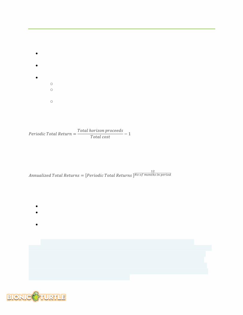
Describe total return analysis, calculate total return, and understand factors present in more sophisticated models.

Monte Carlo simulation and OAS assume that the investor holds the security until maturity. But this may not always be true, as investors have their own horizon.

Total Return Analysis allows investors to evaluate the returns on a security for different investment horizons and interest rate scenarios.

The total returns from an MBS are characterized by the following parameters: o Cost of security at the time of purchase o Security’s projected cash flows (schedules principal payments, interest,

prepayments, and reinvestment income) o Security’s projected value at the horizon date

Example

The total return over a 6-month horizon is calculated using the following formula:

������������������� =�����ℎ��������������

���������− 1

Since these returns are for a 6-month period, the annual returns will be calculated by multiplying them by 2.

Generalized

���������������������� = [��������������������]��

������������������

Factors present in more sophisticated models

In reality, the total return analysis models are highly sophisticated and incorporate many factors:

Models allow returns can be generated in multiple interest rate scenarios. Models allow greater flexibility in generating the inputs. For example, valuation and

prepayment models are utilized to generate horizon price and prepayment rates. The models allow the users to specify when the rate shift happens (immediately, at

horizon, or gradually over time). Culp: “A typical single-name CDS functions almost exactly the same way as credit insurance or a financial guarantee. The credit protection purchaser makes a fixed payment (or a series of fixed payments over time) to the credit protection seller in exchange for a contingent payment upon the occurrence of an event of default by a specific obligation called the reference asset. If the triggering event of default occurs, the credit protection seller makes a cash payment to the protection buyer equal to the par/notional amount of the reference asset minus the expected recovery.”

36

Servigny, Chapter 3: Default Risk: Quantitative Methodologies. Describe the Merton model for corporate security pricing,

including its assumptions, strengths and weaknesses.

Notation:

F = value of debt (as in Face value) S = value of equity (as in Stock) V = value of firm

Under simple (two-class) capital structure, Value of the firm (V) = Value of the debt (F) plus (+) Value of the equity (S) The key insight of Merton model is that equity (shareholders’ claims) is a call option on the firm’s assets. Merton treats the equity claim as a call option on the firm. If the equity holders payoff the debt (i.e., the debt is the exercise price), then they have “exercised” their option and they own the entire firm. But if firm’s assets fall below the value of the debt (or strike price), shareholders essentially hold an “underwater option.”

The value of equity = value of firm’s assets (V) – value of risky debt The value of risky debt = Riskfree debt – put option on firm

The Merton Model’s restrictive assumptions

Simple capital structure: one class of equity + one zero-coupon bond

Value of firm can be observed Value follows a lognormal diffusion

process

Default only occurs at maturity Riskless interest rates are constant Debt is not renegotiated No liquidity adjustment

Capital Structure

Debt(priorclaim)

Equity(residual)

37

Using the Merton model, calculate the value of a firm's debt and equity and the volatility of firm value.

The Merton model for credit treats equity as a call option on the firm’s assets. Under this approach, the value of the equity at date (t) is a function of the value of the firm (V), the face value of the debt (K) and the volatility of the value of the firm ():

( )

2

V N k T t ( )

1log

2

r T tt t V

t V

V

S Ke N k

V K r T t

kT t

Please note this is the same Black-Scholes Merton option pricing model that is reviewed in the Hull assignment; merely the notation is different. Specifically, k = d2.

The Merton model for credit risk has two steps:

(The following breakdown of Merton first appeared in David’s Notebook on our forum at: http://www.bionicturtle.com/forum/threads/merton-model-a-summary-of-the-issues.5646/)

1. Use the Black-Scholes-Merton option-pricing model (BSM OPM) to estimate the price (value) of the firm's equity

2. Using the firm's equity value to assume the firm's asset value and asset volatility, estimate the probability of default (PD) under an assumption that the firm's asset price will follow a lognormal distribution

What’s the role of Black-Sholes-Merton (BSM), here in Merton for credit risk?

The Black-Scholes OPM solves for a European call option = S(0)*N(d1) - K*exp(-rT)*N(d2).

1. BSM OPM is directly applied only in the first step, to get the firm's equity value (and maybe to get the firm's debt)

2. In the second step, N(-d2) is used to estimate PD. It is the same d2, but with one key difference: The riskfree rate (r) in BSM is replaced with a real/physical firm drift (mu). This step uses a component of BSM, so it looks like BSM, but this step is NOT option-pricing at all. It is a simple statistical calculation. Again, N(-d2) is the analog to PD, except real asset drift replaces riskfree rate.

38

What are the two steps, in more detail?

Step 1 (derivatives valuation): price firm equity like a call option

The first step above employs the BSM OPM precisely because its central insight is to treat the firm's equity as a call option on the firm's assets. In this way:

S(0) is replaced by today's firm asset value, V(0), where V(0) = D(0) + E(0); i.e., S(0) in BSM replaced by --> V(0) in Merton

The face value of all debt (not "default threshold" here, that's step 2) replaces the strike price; it's total face value of debt because that is the "strike" that must be paid to retire debt and own the firm's assets. i.e., K or X in BSM replaced by --> F(t) in Merton

We retain the risk-free rate (r) in this step, we do not use the firm's (asset's) expected return. This is theoretically significant: by employing BSM to price equity as a call option, we rely on the brilliant risk-neutral valuation idea, which requires the risk-free rate as the option payoff can be synthesized with riskless certainty. i.e., riskfree rate (r) in BSM is retained in Merton

Summary Step 1:

The Familiar BSM OPM which prices a call option on asset: c(0) = S(0)*N(d1) - K*exp(-rT)*N(d2), is re-purposed to:

Price the firm's equity as if it were an option (strike = debt face value) on firm's assets: E(0) = V(0)*N(d1) - F(t)*exp(-rT)*N(d2)

Two details associated with the first step, that can be skipped

1b. Less important, for FRM exam purposes, is that we solve for both equity value (which informs asset value) and firm asset volatility. The full first step is a simultaneous solution of two equations in two unknowns which produces an assumption for the capital structure (MV of debt + MV of equity = MV of assets) for the firm and the firm's asset volatility. This will not matter in the FRM, it is too tedious. You will instead just be given the assumptions for firm (asset) value and firm (asset) volatility.

1c. More important is that a similar option-based insight can be used to price the value of the firm's debt: the value of the firm's "risky" debt = risk-free debt - put option on firm's assets with strike equal to same face value of debt, where risk-free debt is face value of debt discounted at the risk-free rate.

39

Step 2 (risk measurement): PD = N(-DD)

An FRM P2 candidate should try to understand the relatively simple intuition of this step, which is not option pricing, it is just statistics. Using de Servigny's numbers.

From left-to-right:

Assume current price of assets (i.e., firm value), V(0) = $12.75 Assume assets drift at a rate of mu = +5% per annum At the end of the period, firm will have an expected future value higher than today,

due to positive drift. In this case, V(t) = ~ $13.34 Assume a future distribution, same assumption we use for equities: log returns are

normal --> future prices are lognormal If we are going to make a normal/lognormal assumption, we can treat either, but it

is easier to treat the normal log returns. Our expected future firm value is +28.8% standard deviations above the default threshold = LN(13.34/10) = 28.8%. As our asset volatility is 9.6%, the implies our expected future firm value will be +3 sigma above the default threshold of $10. This final step merely produces a standard normal (Z) variable: LN(13.34/10)/9.6% sigma = Z of ~ 3.0 where 3.0 is the (standardized) distance to default

Under this series of unrealistic assumptions, future insolvency is characterized by a future firm value that is lower than the default threshold of $10; i.e., the area in the tail: PD = N(-DD) = N(-3.0) ~= 0.13%

40

That's Step 2 and the Merton model. Two related ideas:

Risk-free rate (r) vs. asset drift (mu): In BSM, N(d2) = risk-neutral Prob[option expires ITM] and in Merton N(-DD) = risk-neutral Prob[Insolvency; i.e., Asset expires OTM]. BSM risk-neutral d2 = (LN[S(0)/K] + [r - sigma^2/2]*T)/[sigma*SQRT(T)], but Merton's step 2 wants real-world DD = (LN[V(0)/F(t)] + [mu - sigma^2/2]*T)/[sigma*SQRT(T)]

The usage of risk-free rate (r) in the first step and asset drift (mu) in the second step nicely illustrates Jorion's introductory (Chapter 1) distinction between derivatives pricing versus risk measurement. The 1st step above is derivatives pricing. The 2nd step is risk measurement, which he contrasts in five dimensions: 1. distribution of future values, 2. focused on the tail of the distribution [instead of the center, as in step one], 3. Future value horizon, 4. Requires LESS PRECISION (i.e., approximation), and 5. utilizing an ACTUAL (physical) distribution, rather than a risk-neutral

Variation #1: lognormal prices instead of the more familiar normal log returns

The more typical approach, above, derives a standard normal Z deviate by assuming log returns are normally distributed: if LN(S2/S1) is normal then S2 is lognormal. As such, the more typical distance-to-default above produced a standardized normal return-based DD of 3.0 = 28.8% continuous return / 9.6% per annum volatility. In BSM, the numerator of d2 is a continuous return, standardized by dividing by the annualized volatility in the denominator, to give a unitless standard normal deviate.

Alternatively, the distance of default can be expressed as a function of the dollar difference between the future firm asset value and the threshold, in this case: $13.34 - $10 = $3.34. And then standardize that by dividing by the volatility to get the alternative distance to default:

Lognormal price-based Distance to default (DD) = [V(t) - Default]/[sigma*V(t)] = ($13.34 - $10) / (9.6% * $13.34) = 2.607 This price-based lognormal DD of 2.607 is equivalent to the return-based normal DD of 3.0 (normal log returns --> lognormal prices). See row 31 of XLS 6.c.1. for dynamic translation/proof.

41

With respect to the exam (I can't judge the testability of any of this, GARP has been uneven here, overall testability may well be low):

The historical/sample FRM questions tend to query the lognormal price-based DD maybe because it's a shorter formula: [$V(t) - $DefaultPoint]/[sigma*$V(t)]. You'll notice you can't easily retrieve the inverse lognormal CDF, so naturally this sort of questions only asks you the DD and stops short of asking for the PD.

You can confirm with an understanding of the above that this formula wants: Expected future asset value (end of period equity + debt), and The dollar volatility of V(t) is more correct than dollar volatility today [i.e.,

sigma*V(0)] but either is okay. In the simple two-class Merton, MV equity + MV debt = MV of firm assets, V(0) or V(t)

... and debt directly informs the default threshold ... but, otherwise, this DD is entirely a function of firm assets, not equity: asset value today, V(0), drifting at the asset return (mu) to the future expected asset value, V(t), subject to asset volatility, sigma(asset).

Variation #2: KMV (Merton but with two adjustments)

The two steps above illustrate the Merton as (i) assuming the firm will default upon insolvency, asset(t) < face value of all debt(t) and (ii) inferring the area in insolvency tail as a function of a normal return (lognormal price) asset distribution. The KMV method, who I consulted to years ago, recognizes and addresses these two unrealistic assumptions:

1. First, debt consists of short-term obligations (including the short-term portion of long-term debt) and long-term debt. A firm has more time to recover with respect to the long-term debt. KMV's research led it to conclude that the default threshold point is really somewhere in between the short-term debt and the total debt. So, if LT/ST < 1.5, the default threshold = short-term debt + 0.5 * long-term debt.

2. Second, as discussed above, the use of PD = N(-DD) assumes the asset log returns are normally distributed. Let me restate that in, I think, a more meaningful way: by using only the asset volatility, the Merton model tacitly assumes a lognormal distribution of the asset value. As always, this is probably incredibly unrealistic. So, rather than derivate the PD parametrically (i.e., inferring PD as the area under a parametric [lognormal] distribution), KMV resorts to history. Their historical database contains actual firms and their default rates; by back-computing the historical distance-to-defaults, they have a historical correspondence (mapping) of DDs and the actual default rates. For example, whereas parametric normal/lognormal tells us (above) that + 3.0 DD = 0.13% PD (area in the tail), maybe their database shows that +3.0 DD corresponds more nearly to a 0.42% default rate. So, this is a historical empirical translation of DD into PD.

42

In summary, KMV applies Merton (is Merton-based) through 1.5 of the two steps, but abandons the PD = N(-DD) in favor of PD = historical default rate corresponding to DD. Also, KMV tweaks the default threshold from total face value of debt (Merton) to all short-term plus some fraction of long-term debt.

Define the following terms related to default and recovery: default events, probability of default, credit exposure, and loss given default.

Default

Default is failure to pay a financial obligation. Default events include distressed exchanges, in which the creditor receives securities with lower value or an amount of cash less than par in exchange for the original debt. An alternative definition of default is a Merton-type (structural) view of the firm’s

balance sheet: default occurs when the value of the assets drops below the value of the debt, such that equity is reduced to zero or below zero.

Impairment is a weaker accounting concept from the lender’s point of view; a credit can be impaired without default, in which case it is permissible to write down its value and reduce reported earnings by that amount.

According to Malz, “In practice, firms generally file for bankruptcy protection well before their equity is reduced to zero. During bankruptcy, the creditors are prevented from suing the bankrupt debtor to collect what is owed them, and the obligor is allowed to continue business. At the end of the bankruptcy process, the debt is extinguished or discharged. There are a very few exceptions.”

43

Probability of Default

The probability of default is defined over a given time horizon (�); e.g., one year. Each credit has a random default time (t*). The probability of default (p) is the probability of the event (t*) occurs on or before (t); i.e., t* ≤ �. We distinguish three points of time:

The time (t) from which we are viewing default, which is typically “now” or “current” or “initial time;” that is, when t = 0. However, in some cases, we want to think about default probabilities viewed from a future date.

The time interval over which default probabilities are measured: If the perspective time is t = 0, this interval begins at the present time and ends at some future date T, with t = T - 0 = T the length of the time interval. But it may also be a future time interval, with a beginning time T1 and ending time T2,so t = T1 - T2. The probability of default will depend on the length of the time horizon as well as on the perspective time.

The time (t*) at which default occurs. In modeling, this is a random variable, rather than a parameter that we choose.

Credit Exposure

The exposure at default is the amount of money the lender can potentially lose in a default. Exposure can be straightforward (e.g., par or market value of a bond) or a more difficult to ascertain (e.g., the net present value, NPV, of an interest-rate swap contract).

Loss Given Default

When default occurs, in general the creditor does not lose the entire amount of the exposure. The firm’s assets probably have some non-zero value. The firm may be unwound, and the assets sold off, or the firm may be reorganized, so that its assets continue to operate. The loss given default (LGD) is the amount the creditor loses in the event of a default. Exposure is the sum of recovery and loss given default (LGD):

Exposure = Recovery + LGD Recovery is usually expressed as a recovery rate R, a decimal value on [0, 1]:

recoveryrecovery rate(%) =R= 1

exposure exposure

LGD

44

In principle, loss given default (LGD) and recovery are random variables (“random quantities”). As random variables, LGD and recovery (r) create two problems:

1. The uncertainty about LGD makes it more difficult to estimate credit risk 2. The LGD is likely to be correlated with the default probability (PD; aka, EDF) which

adds “an additional layer of modeling difficulty.” In many cases, expected loss (EL) is given as the product of default probability and LGD, but this assumes that LGD is independent of PD.

Recovery rate

The recovery rate can be defined as:

A percent (%) of the current value of an equivalent risk-free bond (recovery of Treasury),

A percent (%) of the market value (recovery of market), or A percent of the face value (recovery of face) of the obligation.

Calculate expected loss from recovery rates, the loss given default, and the probability of default.

The expected loss (EL) is the expected value of the credit loss. From a balance sheet point of view, it is the portion of the loss for which the creditor should be provisioning, that is, treating as an expense item in the income state­ment and accumulating as a reserve against loss on the liability side of the balance sheet. If the only possible credit event is default, then the expected loss is given by:

1 exposureEL R LGD

Loss given default (LGD) and recovery are conditional expectations. This conditional expectation can be expressed by:

loss | defaultdefault

EL ELE LGD

P

45

For example: Expected Loss (EL)

If we assume:

Exposure is $1.0 million, Probability of default (PD) = 1.0%, Loss given default (LGD) = 40.0%; i.e., Recovery rate (R) = 1 – 40.0% = 60.0%

Then the expected loss (EL) = $1.0 million * 1.0% * 40% = $4,000

Additional spread compensates investor for expected loss

Under a simple single-period model, an investor (lender) would require a spread (Z), in addition to the risk-free rate, as compensation for the expected loss:

1 1 1r z R r

Describe the Merton Model, and use it to calculate the value of a firm, the values of a firm’s debt and equity, and default probabilities.

Assumptions of the Merton Model

The Merton Model (which employs the Black-Sholes option pricing model; BS OPM) is arguably the most well-known structural credit risk model. In a structural model, the evolution of the firm’s balance sheet drives credit risk. The Merton Model requires several assumptions:

The value of the firm’s assets, A(t), are assumed to follow a geometric Brownian motion: dAt = µAtdt + σAAtdWt .The market value of the assets, A(t), and the expected return, μ, are related. In equilibrium, if (r) is the riskless continuously compounded interest rate for the same maturity as the firm’s debt, the market’s assessment of the asset value will be such that, given investors’ risk appetites and the distribution of returns they expect, the risk premium (� -r) on the assets is a sufficient reward.

The firm’s balance sheet is “simple” with only one class of debt and one class of equity: At = Et + Dt . Note this is somewhat unrealistic: most firms with marketable debt have different types of issues, with different maturities and different degrees of seniority. But the Merton Model is restrictive: not only is there only one class of debt, but it can only default on the bond’s maturity date.

The debt consists entirely of one issue, a zero-coupon bond with a nominal payment of D, maturing at time T. The notation D, with no subscript, is a constant referring to the par value of the debt. The notation D(t), with a time subscript, refers to the value of the debt at that point in time.

46

Limited liability holds, so if the equity is wiped out, the debtholders have no recourse to any other assets.

Contracts are strictly enforced, so the equity owners cannot extract any value from the firm until the debtholders are paid in full. In reality, when a firm is expected to reorganize rather than liquidate in bankruptcy, there is usually a negotiation around how the remaining value of the firm is distributed to debtholders and equity owners, and all classes may have to lose a little in order to maximize the value with which they all emerge from bankruptcy.

There is trading in the assets of the firm, not just in its equity and debt securities, and it is possible to establish both long and short positions. This precludes intangible assets such as goodwill.

The remaining assumptions are required to “enforce” limited liability: The firm can default only on the maturity date of the bond. There are no cash flows prior to the maturity of the debt; in particular, there are no dividends.

Merton Model formula

The Merton Model is a structural model which assumes that default will happen if and only if, at time (t), the value of the firm’s assets are less than its debt repayment obligation. In short, default will occur if AT < D and the model is given by:

21ln

2t

A

T

A

A

DP A D

The probability of default over the next (T) years is therefore the probability that the Brownian motion A(t) hits the level (D) within the interval [0, T(0)]. The quantity A(T) - D is called the distance to default. In this setup, we can view both the debt and equity securities as European options on the value of the firm’s assets, maturing at the same time (T) as the firm’s zero-coupon debt. We can value the options using the Black-Scholes Merton option pricing model. The model will then help us obtain estimates of the probability of default and

Equity value of the firm. Although they are hard to generate in practice, we treat as known the current value of the firm’s assets, A(t), and the volatility of the assets, σ(A). The equity can then be treated as a call option on the assets of the firm A(t) with an exercise price equal to the face value of the debt (D). If, at the maturity date (T) of the bond, the asset value A(T) exceeds the nominal value of the debt (D), the firm will pay the debt. If, in contrast, we have A(T) < D, the owners of the firm will be wiped out, and the assets will not suffice to pay the debt timely and in full.

47

The equity value at maturity is therefore E(T) = MAX[A(T) - D,0]. We can the value the firm’s equity as a call on its assets, struck at the value of the debt: E(T) = v[A(t), D, t, (A),r,0]

Market value of the debt. We can also apply option theory from the point of view of

the lenders. We can treat the debt of the firm as a portfolio consisting of a risk-free bond with par value (D) plus (+) a short position in a put option on the assets of the firm, A(t), with exercise price D. The present value of the risk-free bond is D*exp(-rt), such that the future value of the debt is given by: D(T) = D – MAX[D – A(T), 0]

Denoting the Black-Scholes value of a European put w[A(t), D, t, σ(A), r, 0] we have the current value of the bond, as adjusted for risk by the market: D(t) = exp(-rt)*D - w[A(t),D, tτ,σσ(A), r, 0]

Firm’s Balance Sheet: The firm’s balance sheet can be expresses in terms of put-call parity: A(t) = E(t) + D(t) = v[A(t), D, t, σ(A), r, 0] + exp(-rt)*D - w[A(t),D,τt, σ(A), r, 0]

Describe credit factor models and evaluate an example of a single-factor model.

Factor models can are a type of structural model since they try to relate the risk of credit loss to fundamental economic quantities. In contrast to other structural models, however, the fundamental factors have their impact directly on asset returns, rather than working through the elements of the firm’s balance sheet.

Single-factor model

A simple but widely used type is the single-factor model. The model is designed to represent the main motivating idea of the Merton model—a random asset value, below which the firm defaults—while lending itself well to portfolio analytics.

48

The firm’s asset return is represented as a function of two random variables: the return on a “market factor” (m) that captures the correlation between default and the general state of the economy, and a shock, e(i), capturing idiosyncratic risk. However, the fundamental factor is not explicitly modeled: It is latent; i.e., its impact is modeled indirectly via the model parameters. The single-factor model is given by:

2single-factor model: 1

~ (0,1)

~ (0,1)

[ , ] 0

Ta m

where

m N

N

Cov m

Under these assumptions (a) is a standard normal variate. Since both the market factor and the idiosyncratic shocks are assumed to have unit variance (since they’re standard normals), the beta of the firm’s asset return to the market factor is equal to β:

2 2

[ ] 0

[ ] 1 1

T

T

E a

Var a B

Define Credit VaR (Value-at-Risk).

Both credit value-at-risk (CVaR) and market value-at-risk (VaR) are quantiles of a distribution (and unexpected loss, UL, is the quantile of the credit loss in excess of the expected loss), but although mathematically similar, there are at least two realistic differences between measuring credit and market risk:

1. The time horizons for market risk are “almost always between one day and one month.” But the typical time horizon for measuring credit risk is much longer; often, as in the case of the Basel Accord, the credit risk horizon is one year.

Consequently, for expected credit returns, the credit “drift,” cannot be assumed to be zero (unlike for market risk, where for a ten-day horizon, drift is often assumed to be zero). Credit returns have additional issues that do not quite arise identically for market risk, involving the treatment of promised coupon payments and the cost of funding positions.

2. Credit return distributions exhibit extreme skewness. For most unleveraged

individual credit-risky securities and credit portfolios, the overwhelming likelihood is that returns will be relatively small in magnitude, driven by interest payments made on time or by ratings migrations. But on the rare occasions of defaults or clusters of defaults, returns are large and negative. In contrast, market returns (especially over a short horizon) are often less skewed due the potential for upside.

49

Because of the skewness of credit portfolios, the confidence level for credit VaR measures tend to be somewhat higher than for market risk; while 95.0% is not unusual for market risk VaR, CVaR is often calibrated at 99.9% confidence.

Expected and Unexpected Loss

Credit losses can be decomposed into three components: Expected loss (EL) Unexpected loss (UL), and The extreme loss “in the tail” beyond the unexpected loss

Unexpected loss (UL) is a quantile of the credit loss in excess of the expected loss.

UL is sometimes defined as one standard deviation (e.g., Ong defines UL thusly) but sometimes as the 99th or 99.9th percentile of the loss in excess of the expected loss.

According to Malz, “The standard definition of credit Value-at-Risk is cast in terms of UL: It is the worst case loss on a portfolio with a specific confidence level over a specific holding period, minus the expected loss.”

50

Malz, Chapter 7: Spread Risk and Default Intensity Models. Define the different ways of representing spreads. Compare and differentiate between the different spread conventions and compute one spread given others when possible.

There are different ways to represent a credit spread although, according to Malz, all of the following metrics decompose bond interest into (i) a component that is compensation for credit and liquidity risk and (ii) a component that is compensation for the time value of money (TVM):

Yield spread: the difference between the yield to maturity (YTM) of a risky bond and the YTM of a benchmark government bond with the same (or approximately the same maturity). In short, yield spread = YTM[risky bond] – YTM[riskless government bond | similar maturity]. Yield spread is commonly used in price quotes, but less so for fixed-income analysis.

Interpolated spread (i-spread): The benchmark government bond (or a freshly initiated plain vanilla interest-rate swap) almost never has the same maturity as a particular credit-risky bond; the maturities can be very different. The i-spread is the difference between the yield of the credit-risky bond and the linearly interpolated yield between the two benchmark government bonds or swap rates with maturities flanking that of the credit-risky bond. It is commonly used, like yield spread, for price quotes.

Zero-coupon (z-spread) is the spread that must be added to the LIBOR spot curve to arrive at the market price of the bond; however, it may also be measured relative to a government bond curve. Therefore, it is good practice to specify the reference risk-free curve being used.

,

1

( ) ih

hr z ih r z

hi

p c ch e e

Asset-swap spread is the spread or quoted margin on the floating leg of an asset swap on a bond.

Credit default swap spread is the market premium, expressed in basis points, of a CDS on similar bonds of the same issuer.

Option-adjusted spread (OAS) is a version of the z-spread that takes account of options embedded in the bonds. If the bond contains no options, OAS is identical to the z-spread.

Discount margin (a.k.a., quoted margin) is a spread concept applied to floating rate notes. It is the fixed spread over the current (one-or three-month) LIBOR rate that prices the bond precisely. The discount margin is thus the floating-rate note analogue of the yield spread for fixed-rate bonds.

51

Explain how default risk for a single company can be modeled as a Bernoulli trial.

Default risk for a single company can be represented as a Bernoulli trial. Over some fixed time horizon (�) =T2 – T1, there are just two outcomes for the firm:

Default occurs with probability (π) The firm remains solvent with probability (1- π)

If we assign the values 1 and 0 to the default and solvency outcomes over the time interval (T1,T2], we define a random variable that follows a Bernoulli distribution. The time interval (T1,T2] is important: The Bernoulli trial does not ask “does the firm ever default?,” but rather, “does the firm default over the next year?” The mean and variance of a Bernoulli-distributed variable are easy to compute:

The expected value of default on (T1,T2] is equal to default probability π and The variance of default is π * (1- π)

Binomial is a series of Bernoulli trials

If Bernoulli trials can be repeated during successive time intervals, of identical length �, and where the probability of default during each interval is a constant value �, then we can say the trials are conditionally independent (a.k.a., the model has the property of memorylessness). This series of independent and identically (i.e., same probability of default) distributed Bernoulli trials is characterized by a binomial distribution.

Define the hazard rate and use it to define probability functions for default time and conditional default probabilities.

The hazard rate is also called default intensity and is denoted by lambda, λ. We can interpret the hazard rate as the instantaneous conditional default probability.

Default time distribution function

The default time distribution function or cumulative default time distribution function is the probability of default sometime between now and time (t) and is given by:

[ * ] ( ) 1 tP t t F t e The survival and default probabilities must sum to exactly 1.0 at every instant (t), so the probability of no default sometime between now and time t, called the survival time distribution, is given by:

52

[ * ] 1 [ * ] 1 ( ) tP t t P t t F t e The survival probability converges to 0 and the default probability converges to 1.0 as (t) grows very large: in the intensity model, even a “bullet-proof” AAA-rated company will default eventually. This remains true even when we let the hazard rate vary over time.

Default time density function

The default time density function or marginal default probability is the derivative of the default time distribution w.r.t. t:

[ * ] ( ) tP t t F t et

This is always a positive number, since default risk “accumulates;” i.e., the probability of default increases for longer horizons. If lambda, λ, is small, it will increase at a very slow pace. The survival probability, in contrast, is declining over time:

[ * ] ( ) 0tP t t F t et

With a constant hazard rate, the marginal default probability is positive but declining.

Conditional default probability

If we ask, what is the probability of default over some horizon (t, t + � ) given that there has been no default prior to time (t), we are asking about a conditional default probability. By the definition of conditional probability, it can be expressed as the ratio of the probability of the joint event of survival up to time (t) and default over some horizon (t, t + � ), to the probability of survival up to time (t):

* *

* | **

P t t t tP t t t t

P t t

Calculate risk-neutral default rates from spreads.

The spread is approximately equal to the default probability multiplied by the loss given default (LGD), such that the hazard rate is approximated by the spread divided by (1-R):

* *(1 )1

zz R

R

53

Define default correlation for credit portfolios.

Default correlation drives the likelihood of having multiple defaults in a portfolio of debt issued by several obligors. The simplest framework for understanding default correlation is the case of only two firms (or obligors or credits). The assumptions are:

Two firms (or countries, if we have positions in sovereign debt). With respective probabilities of default = π(1) and π(2) Over some time horizon (t) And a joint default probability (i.e., the probability that both default over t) equal to

π(12) Then the default correlation, ρ(12), is given by:

12 1 2

12

1 1 2 21 1

Describe how a single factor model can be used to measure conditional default probabilities given economic health.

To use the single-factor model to measure portfolio credit risk, we start with a number of firms i =1,2, ... , where each firm has:

Its own correlation β(i) to the market factor, its own standard deviation of idiosyncratic risk, SQRT[1- β(i)^2], and its own idiosyncratic shocke(i)

Firm (i)’s return on assets is given by:

21 1, 2,i i i ia m i

We assume (m) and e(i) are standard normal variates, and further are not correlated with one another. In addition assume thee(i) are not correlated with one another:

~ (0,1)

~ (0,1) 1, 2,...

, 0 1, 2,...

, 0 , 1, 2,...

i

i

i j

m N

N i

Cov m i

Cov i j

54

Under these assumptions, each a(i) is a standard normal variate. Since both the market factor and the idiosyncratic shocks are assumed to have unit variance, the beta of each credit (i) to the market factor is equal to β(i). The correlation between the asset returns of any pair of firms (i) and (j) is β(i)β(j):

2 2

2 2

0 1, 2,...

1

, 1 1

i

i i i

i j i i i i i i i j

E a i

Var a

Cov a a E m m

Compute variance of the conditional default distribution and conditional probability of default using single-factor model.

To summarize, specifying a realization � = �� does three things:

1. The conditional probability of default is greater or smaller than the unconditional probability of default, unless either �� = 0���� = 0, that is, either the market factor shock happens to be zero, or the firm’s returns are independent of the state of the economy. There is also no longer an infinite number of combinations of market and idiosyncratic shocks that would trigger a firm default. Given �� , a realization of �� less than or equal to �� − ����(�= 1,2, … . ) triggers default. This expression is linear and downward sloping in �� : as we let �� vary from high (strong economy) to low (weak economy) values, a smaller, a smaller (less negative) idiosyncratic shock will suffice to trigger default.

2. The conditional variance of the default distribution is 1 − ���, so the conditional

variance is reduced from the unconditional variance of 1.

3. It makes the asset returns of different firms independent. The �� are independent, so

the conditional returns �1− ����� and �1− ��

��� and thus the default outcomes for

two different firms (i) and(j) are independent. Putting this all together, while the unconditional default distribution is a standard normal, the conditional distribution can be represented as a normal with a mean of −���� and a

standard deviation of �1− ���.

55

The conditional cumulative default probability function can now be represented as a function of (m):

2( ) 1, 2,

1

i i

i

k mp m i

Explain how Credit VaR of a portfolio is calculated using the single-factor model, and how correlation affects the distribution of loss severity for intermediate values between 0 and 1.

Recall that, for a given realization of the market factor, the asset returns of the various credits are independent standard normals. That, in turn, means that we can apply the law of large numbers to the portfolio. For each level of the market factor, the loss level x(m), that is, the fraction of the portfolio that defaults, converge to the conditional probability that a single credit defaults, given for any credit by

2( )

1

k mp m

Gregory, Chapter 2: Defining Counterparty Credit Risk

We can define exposure as: Exposure = Max (MtM, 0) = MtM+ Counterparty risk creates an asymmetric risk profile that can be likened to a short option position:

Since exposure is similar to an option payoff, a key aspect will be volatility of the MtM

Options are relatively complex to price (compared with the underlying instruments at least). Hence, to quantify credit exposure even for a simple instrument may be quite complex

Potential future exposure (PFE)

The concept of potential future exposure (PFE) arises from the need to characterize what the MtM might be at some point in the future. PFE defines a possible exposure to a given confidence level, normally according to a worst case scenario. PFE over a given time horizon is analogous to the traditional value at-risk.

56

PFE is characterized by the fact that the MtM of the contract(s) is known both at the current time and at any time in the past. However, there is uncertainty over the future exposure that might take any one of many possible paths as shown. At some point in the future, one will attempt to characterize PFE via some probability distribution.

Define the following metrics for credit exposure: expected mark-to-market, expected exposure, potential future exposure, expected positive exposure, effective exposure, and maximum exposure.

Expected mark-to-market

Expected mark-to-market (MtM) represents the forward or expected value of a transaction at some point in the future. Due to the relatively long time horizons involved in measuring counterparty risk, the expected MtM can be an important component, whereas for market risk VAR assessment (involving only a time horizon of 10 days), it is typically not. Expected MtM may vary significantly from current MtM due to the specifics of cash flows. Forward rates are also a key factor when measuring exposure under the risk-neutral measure

Expected exposure (EE)

Due to the asymmetry of losses, an institution typically cares only about positive MtM values since these represent the cases where they will make a loss if their counterparty defaults. Hence, it is natural to ask what the expected exposure (EE) is since this will represent the amount expected to be lost if the counterparty defaults. By definition, the EE will be greater than the expected MtM since it concerns only the positive MtM values

-60% -40% -20% 0% 20% 40% 60%

Probability

EE

PFE

Mean

57

Potential future exposure (PFE)

In risk management, it is natural to ask ourselves what is the worse exposure we could have at a certain time in the future? A PFE will answer this question with reference to a certain confidence level. For example, the PFE at a confidence level of 99% will define an exposure that would be exceeded with a probability of no more than 1% (one minus the confidence level). PFE is exactly the same as the traditional measure of value-at-risk (VAR) with two notable exceptions:

PFE may be defined at a point far in the future (e.g. several years) whereas VAR typically refers to a short (e.g. 10-day) horizon.

PFE refers to a number that will normally be associated with a gain (exposure) whereas traditional VAR refers to a loss. VAR is trying to predict a worst-case loss whereas PFE is actually predicting a worst-case gain since this is the amount at risk if the counterparty defaults.

The previous exposure metrics are concerned with a given time horizon. The following metrics characterize exposure through time.

Expected positive exposure (EPE)

Expected positive exposure (EPE) is defined as the average EE through time and hence can be a useful single number representation of exposure.

EPE has a strong theoretical basis for pricing and assessing portfolio counterparty risk

Effective EPE

Effective EPE is the average of the effective EE: Effective EE is simply a non-decreasing EE. Measures such as EE and EPE may underestimate exposure for short-dated transactions (since capital measurement horizons are typically 1-year) and not capture properly rollover risk (Chapter 3). For these reasons, the terms effective EE and effective EPE were introduced by the Basel Committee on Banking Supervision (2005).

Maximum PFE

Maximum PFE simply represents the highest (peak) PFE value over a given time interval. Such a definition could be applied to any exposure metric but since it is a measure that would be used for risk management purposes, it is more likely to apply to PFE.

58

Describe the parameters used in simple single-factor models …

Equities

The standard model for equities is a geometric Brownian motion (GBM) as defined by:

( ) ( )tE t

t

dSt dt t dW

S

Where S(t) represents the value of the equity at time (t), μ(t) is the drift, �(t) is the volatility and dW(t) is a standard Brownian motion. GBM assumes that the log returns are normally distributed.

The drift may be chosen to be positive or negative to reflect a conservative assumption based on the transactions involved or it may be set to the risk-free rate plus some risk premium (as defined by the capital asset pricing model).

The volatility could also be either market-implied or determined from historical analysis.

For practical purposes, it may not be advisable to attempt to simulate every single underlying stock. Not only is this highly time-consuming but it also leads to a large correlation matrix that may not be of the appropriate form. Rather, one may choose to simulate all major indices and then estimate the change in the individual stock price by using the beta of that stock, assuming a correlation of 100% between the stock and index (this may often represent a conservative approximation).

FX

In a traditional model for FX rates, X(t), is to assume a standard geometric Brownian motion (GBM) as for equities:

( ) ( )tFX t

t

dXt dt t dW

X

This ensures that FX rates are always positive. The drift, μ(t), can be calibrated to the forward rates or determined via historical analysis as discussed above. One could also consider adding some mean reversion to avoid FX rates becoming unrealistically large or small, especially for long time horizons. The equation can then be re-written:

ln ( )tFX t

t

dXk X dt t dW

X

59

Where (k) is the rate of mean reversion to a long-term mean level. This long-term mean may be set at the current spot level or set to a different level due to the view of a risk manager, historical analysis, forward rates or simply to be conservative. Whilst it is conservative to ignore mean reversion, in such a model long-term FX rates can arguably reach unrealistic levels.

Commodities

Commodities tend to be highly mean reverting around a level, which represents the marginal cost of production. Furthermore, many commodities exhibit seasonality in prices due to harvesting cycles and changing consumption throughout the year. A simple and popular model for commodities is given by:

ln ( ) ( )

( ) ( ) ( )

t

C t

S f t Z t

dZ t Z t dt t dW

Where f(t) is a deterministic function, which may be expressed using sin or cos trigonometry functions to give the relevant periodicity and the parameters and are the mean reversion parameters. For commodities, the use of risk-neutral drift is particularly dangerous due to the strong backwardation and contango present for some underlyings. However, non-storable commodities (for example, electricity) do not have an arbitrage relationship between spot and forward prices and therefore the forward rates might be argued to contain relevant information about future expected prices.

Credit spreads

Credit products have significant wrong-way risk and so a naive modeling of their exposure without reference to counterparty default is dangerous. Credit spreads, like the above asset classes, require a model that prevents negative values. They also, more than any other asset class, might be expected to have jumps caused by a sudden and discrete change in credit quality (such as an earnings announcement or ratings downgrade or upgrade). An approach that fits these requirements is the following model:

t t t td dt dW j dN

where �(t) is the intensity (or hazard rate) of default and � and � are mean reversion parameters. Additionally, dN represents a Poisson jump with jump size (j). This jump size can itself be random such as following an exponential distribution.

60

Interest rates

Interest rates may be one asset class where we may be willing to allow negative rates to provide the benefit of tractability. The simplest interest rate model s the one-factor Hull and White (or extended Vasicek) model (Hull and White, 1990) where the ‘‘short rate’’ (short-term interest rate) is assumed to follow the following process:

( )t t r tdr t ar dt dW

In this model, the short rate follows a Brownian motion with mean reversion. Mean reversion dictates that when the rate is above some ‘‘mean’’ level, it is pulled back towards that level with a certain force according to the size of parameter. The mean reversion level, � (t), is time-dependent which is what allows this model to be fitted to the initial yield curve. The parameters can then be calibrated to market data or estimated from historical data. Mean reversion has the effect of damping the standard deviation of discount factors, B(t,T).

Describe how netting is modeled.

A netting agreement allows two parties to net a set of positions (explicitly covered by the netting agreement) in the event of default of one of them. This is a critical way to control exposure but can typically only be quantified effectively in a Monte Carlo framework. Netting benefits arise in scenarios where the MtM values of two trades are of opposite signs. Hence, to calculate the impact of netting one must aggregate at the individual transaction level. We cannot add exposure metrics (such as EE) to incorporate the impact of netting. Netting must be incorporated before calculating quantities such as EE. In order to calculate the new exposure of a netting set when a trade indexed by m+1 has been added, we needs to calculate the expression:

', , , 1, ,

1

max ,0n

j k i j k m j ki

E V V

61

Define and calculate the netting factor.

We can use the EPE to define a ‘‘netting factor’’ as:

(netting)netting factor

(without netting)

EPE

EPE

The above measure will be +100% if there is no netting benefit and 0% if the netting benefit is maximum. Note that a single time horizon netting factor is defined by EE whereas a time-averaged value is defined using EPE.

Define and calculate marginal expected exposure and the effect of correlation on total exposure.

Suppose we have calculated a netted exposure for a set of trades under a single netting agreement. We would like to be able to write the total EE as a linear combination of EEs for each trade, i.e.:

*

1

n

total ii

EE EE

If there is no netting then we know that the total EE will indeed be the sum of the individual components and hence the marginal EE will equal the EE:

*if no netting then i iEE EE However, since the benefit of netting is to reduce the overall EE, we expect in the event of netting that marginal (EE) < individual (EE). In the case of perfectly offsetting exposures, the marginal EEs must sum to zero.

Gregory, Chapter 5: Quantifying Counterparty Credit Exposure, II: The Impact of Collateral. Calculate the expected exposure and potential future exposure over the remargining period given normal distribution assumptions.

If we assuming that a netted set of trades is perfectly collateralized at a given time and the change in the netted exposure (and collateral value) follows a normal distribution with zero mean and volatility parameter, where T(M) denotes the remargin period of the risk, the expected exposure (EE) is given by

10.4

2E M E MEE T T

62

And the potential future exposure at a given confidence level alpha(�) is given by:

1( ) E MPFE T

The above formula is analogous to a VAR formula under a normal distribution assumption of portfolio value

E MPFE k T

Define and calculate credit value adjustment (CVA) when no wrong-way risk is present.

If we assume independence between default probability, exposure and recovery, we are ignoring wrong-way risk. Under this simplifying assumption (i.e., no wrong-way risk) the simplified credit value adjustment (CVA) expression is given by:

11

1 ,m

j j j jj

CVA B t EE t q t t

CVA depends on the following components:

Loss given default (LGD): LGD = (1-recovery rate). This is the percentage amount of the exposure expected to be lost if the counterparty defaults.

Discount factors. The expression B(t[j]) gives the risk-free discount factor at time t[j]. This is relevant since any future losses must be discounted back to the current time. It is sometimes hard to obtain risk-free discount factors that are not contaminated with some credit risk component and it should be emphasized that LIBOR rates have sometimes been above Treasury bond yields.

Expected exposure (EE). The term EE(t[j]) is the expected exposure (EE) for the relevant dates in the future given by t[j] for j = 0, n m.

Default probability. The expression q(t[j-1], t[j]) gives the marginal default probability in the interval between date t[j+1] and t[j].

63

Describe the process of approximating the CVA spread.

Suppose that instead of computing the CVA as a stand-alone value, we want to express it as a running spread (per annum charge). A simple calculation would involve dividing the CVA by the risky annuity for the maturity in question The formula assumes additionally that the EE is constant over time and equal to its average value (EPE). This yields the following approximation based on this EPE:

premium

( , )

( , )CDSCVA t T

X EPECDS t T

where CDS[premium](t,T) is the unit premium value of a CDS (risky annuity) and X(CDS) is the CDS premium corresponding to the maturity date (T) and can be viewed as a credit spread. The above equation (Gregory 7.2) will work well in the following cases:

EPE is reasonably constant over the whole profile. Default probability is reasonably constant over the whole profile. Either EE or default probability is symmetric over the whole profile such that there is

a cancellation effect similar to that in the example above.

Define and calculate the incremental CVA and the marginal CVA.

To consider the impact of netting, the change in CVA, i.e. the CVA before and after a new trade has been executed, must be assessed. A new trade should be priced so that its profit at least offsets any increase in CVA. In other words, the risky value of the netted derivatives positions must not change. We can derive the following formula:

,( ) ( , ) ( ) NS iV i CVA NS i CVA NS CVA

Where V(i) gives the risk-free value of the new trade (i), CVA(NS) is the CVA on all existing trades within the same netting set and CVA(NS,i) is the CVA included in the new trade in the netting set. Due to the properties of netting we must have ΔCVA(NS,i) ≤ CVA(i); i.e., the impact trade (i) has on the netting set CVA must be no more than its individual CVA. The above equation defines that the profit (loss) made on the transaction must offset the increase (decrease) in the total CVA when adding the new trade. If the increase in CVA is negative (due to favorable netting effects), it may be possible to execute a trade at a loss due to the overall gain from CVA reduction. To price a new trade with the impact of netting, one must calculate the change in CVA, termed the incremental CVA that the new trade will create. As with the case of collateral,

64

this depends only on the EE and hence virtually the same formula as before will apply with just the incremental EE (�EE) replacing the EE:

11

1 ,m

j j j jj

CVA B t EE t q t t

Where ΔEE(t[j]) represents the incremental change in EE at each point in time caused by the new trade while the other terms are defines per the CVA formula (with no wrong-way risk).

Incremental CVA

Incremental CVA is analogous to incremental expected exposure (EE). The incremental CVA(i) is given by the incremental effect of a trade on the netting set:

incrementali NS i NSCVA CVA CVA

The incremental CVA is never higher than the standalone CVA.

Marginal CVA

Incremental risk measures are not additive: it is not possible to split the CVA numbers up into additive components. This makes it difficult to price trades transacted at the same time (perhaps due to being part of the same deal) with a given counterparty. By using a marginal CVA measure, it will be possible to break down a CVA for any number of netted trades into trade level contributions that sum to the total CVA.

Define and calculate CVA and CVA spread in the presence of a bilateral contract.

Bilateral CVA

A recent trend has been to consider the bilateral nature of counterparty risk. This means that an institution would consider a CVA calculated under the assumption that they, as well as their counterparty, may default. The definition of bilateral CVA (BCVA) follows directly from that of unilateral CVA with the assumption that the institution concerned can also default. We obtain the following expression under the assumption of no simultaneous defaults or wrong-way risk:

1 11

1 11

1 ,

1 ,

m

i i I i i ii

m

I i i i I i ii

BCVA B t EE t S t q t t

B t NEE t S t q t t

65

The second BCVA term is a mirror image of the first term and represents a negative contribution – this is often known as DVA (debt value adjustment). It corresponds to the fact that in cases where the institution defaults (before their counterparty), they will make a ‘‘gain’’ if the MtM is negative (a ‘‘negative exposure’’). A gain in this context might seem unusual but it is, strictly speaking, correct since in default the institution will pay their counterparty only a fraction (recovery) of what they owe them. (Using the Sorensen and Bollier analogy, the institution is then also long a series of swaptions.)

Crouhy Chapter 14: Describe RAROC (risk-adjusted return on capital) methodology

The benefits of the RAROC methodology include: RAROC provides a common and consistent economic yardstick for measuring risk,

which includes an economic basis for measuring all the relevant risk types and risk positions consistently (including the authority to incur risk)

RAROC generates risk/reward signals at all levels of the business. Because RAROC promotes consistent, fair, and reasonable risk-adjusted performance measures, it provides managers with the information that they need to make the trade-off between risk and reward more efficient.

RAROC analysis reveals how much economic capital is required by each business line, product, or customer

Risk-adjusted return on capital (RAROC)= Risk-adjusted return / EC

In this context, risk-adjusted return is potentially confusing: it is not fully risk-adjusted. Rather, ARAROC is truly risk-adjusted. In this narrow context, risk-adjusted merely implies that expected losses are accounted for. In this sense, we would argue that the denominator of RAROC is risk-adjusted but the numerator is not.

Economic capital (EC), unless otherwise specified, refers to capital buffer against unexpected losses (UL) excluding expected losses (EL)

Unexpected losses (UL) and economic capital (EC), are a function of confidence level; i.e., higher confidence (lower significance) implies higher UL and higher EC. In this way, OpRisk VaR is similar to Market Risk VaR, except the distributions are different and the “drift” is an expected loss.

66

Note the ratio consistency in RAROC: subtract EL in numerator and exclude EL in denominator (it would be okay to add EL back in both, but this author does not):

excludeRisk-adjusted return

Economic Capital

s EL

excludes ELRAROC

Compute and interpret the RAROC for a loan or loan portfolio, and use RAROC to compare business unit performance.

RAROC ratio:

Numerator = Revenue + Return on Invested Capital (ROC) – [Cost of Funds (COF) + Operating Expenses (OpExp)] – Expected Losses (EL)

Denominator = Economic capital

Revenues ROC (COF OpExp) EL

Economic CapitalRAROC

67

Explain how the second-generation RAROC approaches improve economic capital allocation decisions

The problem with RAROC is that, given a fixed hurdle rate of return, RAROC might to decide to accept a project that is too risky. The appendix math shows this is essentially similar to accepting projects due to a high ROE, without adjusting for the true (risky) cost of capital. The problems with RAROC are:

RAROC is sensitive to the level of the standard deviation of the risky asset. So

RAROC may indicate that a project achieves the required hurdle rate, given a high enough volatility, even when the net present value of the project is negative

RAROC is sensitive to the correlation of underlying asset’s return and the market portfolio

If a fixed hurdle rate is used in conjunction with RAROC, high-volatility and high-correlation projects will tend to be selected

The second-generation RAROC is called Adjusted RAROC (ARAROC) and ARAROC overcomes these problems:

The ARAROC measure is insensitive to changes in volatility and correlation. Adjusted RAROC is given by:

FRAROC-R

ARAROCE

RF is the risk free rate

E is the systematic risk of equity

(beta)

68

Compute the adjusted RAROC for a project to determine its viability.

The project should be accepted if the adjusted RAROC exceeds the market’s equity risk premium; i.e., accept if ARAROC > E[Market return] – Riskfree rate

For example: Given the following assumptions:

Riskless rate = 4%, Market return = 9%, such that Equity risk premium (ERP) = 9% - 4% = 5%, and The firm’s equity beta = 1.2.

First scenario. Assume project’s RAROC is 11.0%, then:

11%-4%

ARAROC= 5.83%1.2

Because 5.83% is greater than the market equity premium of 5%, the project should be accepted.

Second scenario. Assume project’s RAROC is only 9%, then:

9%-4%

ARAROC= 4.17%1.2

And now the project should be rejected, because 4.17% < ERP of 5.0%. In this case, the project’s expected return is equal to the market’s return of 9%, but the firm is riskier than the market (as measured by the beta) and so the firm has a higher cost of capital.

69

Ideal risk measure

An ideal risk measure should be intuitive, stable, easy to compute, easy to understand, coherent and interpretable in economic terms. Additionally, risk decomposition based on the risk measure should be simple and meaningful.

Intuitive: The risk measure should meaningfully align with some intuitive notion of risk, such as unexpected losses.

Stable: Small changes in model parameters should not produce large changes in the estimated loss distribution and the risk measure. Similarly, another run of a simulation model in order to generate a loss distribution should not produce a dramatic change in the risk measure. Also, it is desirable for the risk measure not to be overly sensitive to modest changes in underlying model assumptions.

Easy to compute: The calculation of the risk measure should be as easy as possible. In particular, the selection of more complex risk measures should be supported by evidence that the incremental gain in accuracy outweighs the cost of the additional complexity.

Easy to understand: The risk measure should be easily understood by the bank’s senior management. There should be a link to other well-known risk measures that influence the risk management of a bank. If not understood by senior management, the risk measure will most likely not have much impact on daily risk management and business decisions, which would limit its appropriateness.

Coherent: The risk measure should be coherent and satisfy the conditions of: i. Monotonicity (if a portfolio Y is always worth at least as much as X in all

scenarios, then Y cannot be riskier than X); ii. Positive homogeneity (if all exposures in a portfolio are multiplied by the same

factor, the risk measure also multiplies by that factor); iii. Translation invariance (if a fixed, risk-free asset is added to a portfolio, the risk

measure decreases to reflect the reduction in risk); and iv. Subadditivity (the risk measure of two portfolios, if combined, is always

smaller or equal to the sum of the risk measures of the two individual portfolios). Of particular interest is the last property, which ensures that a risk measure appropriately accounts for diversification.

Simple and meaningful risk decomposition (risk contributions or capital allocation): In order to be useful for daily risk management, the risk measured for the entire portfolio must be able to be decomposed to smaller units (e.g., business lines or individual exposures). If the loss distribution incorporates diversification effects, these effects should be meaningfully distributed to the individual business lines

70

Types of risk measures (Table 1)

Standard Deviation VaR

Expected Shortfall

Spectral and Distorted Risk Measures

Intuitive Sufficiently intuitive

Yes Sufficiently intuitive

No (involves choice of function)

Stable No, depends on loss distribution assumptions

No, depends on loss distribution assumptions

Depends on loss distribution

Depends on loss distribution

Easy to compute

Yes Sufficiently easy (requires estimate of loss distribution)

Sufficiently easy (requires estimate of loss distribution)

Sufficiently easy (weighting of loss distribution by spectrum/distortion function)

Easy to understand

Yes Yes Sufficiently Not immediately understandable

Coherent Violates monotonicity

Violates subadditivity

Yes Yes

Simple and meaningful risk decomposition

Simple but not very meaningful

Not simple, might induce distorted choices

Relatively simple and meaningful

Relatively simple and meaningful

71

Calculation of risk measures

Confidence level: The link between a bank’s target rating and the choice of confidence level may be interpreted as the amount of economic capital that must be exceeded by available capital resources to prevent the bank from eroding its capital buffer at a given confidence level (a so-called “going concern view”). Banks typically use different confidence levels for different purposes; the choice of a confidence level might differ based on the question to be addressed. On the one hand, high confidence levels reflect the perspective of creditors, rating agencies and supervisors in that they are used to determine the amount of capital required to minimize bankruptcy risk. On the other hand, banks may use lower confidence levels for management purposes in order to allocate capital to business lines and/or individual exposures and to identify those exposures that are critical for profit objectives in a normal business environment.

Time Horizon: All risk measures depend on the time horizon used in their measurement. The choice of an appropriate time horizon depends on a range of factors: the liquidity of the bank’s assets under consideration; the risk management needs of the bank, the bank’s standing in the markets; the risk type, etc.

Market risk is typically estimated over a very short time horizon (days or weeks). In contrast, credit risk is typically measured using a one-year time horizon, while an even longer time horizon may be appropriate for other portfolios (e.g., project finance). The choice of time horizon is also influenced by regulatory requirements.

Risk aggregation methodologies

Banks differ in their choice of methodology for the aggregation of economic capital. The list below provides an overview of the main approaches followed by a brief discussion of their advantages and disadvantages. The approaches are listed in increasing order of complexity (decreasing order of restrictiveness).

i. Simple summation: This simple approach involves adding the individual risk components. Typically, this is perceived as a conservative approach since it ignores potential diversification benefits and produces an upper bound to the true economic capital figure. Technically, it is equivalent to assuming that all inter-risk correlations are equal to one and

72

ii. Applying a fixed diversification percentage: This approach is essentially the same as the simple summation approach with the only difference that it assumes the sum delivers a fixed level of diversification benefits, set at some pre-specified level of overall risk.

iii. Aggregation on the basis of a risk variance-covariance matrix: The approach allows for a richer pattern of interactions across risk types. However, these interactions are still assumed to be linear and fixed over time. The overall diversification benefit depends on the size of the pairwise correlations between risks.

iv. Copulas: This is a much more flexible approach to combining individual risks than the use of a covariance matrix. The copula is a function that combines marginal probability distributions into a joint probability distribution. The choice of the functional form for the copula has a material effect on the shape of the joint distribution and can allow for rich interactions between risks.

v. Full modelling of common risk drivers across all portfolios: This represents the theoretically pure approach. Common underlying drivers of risk are identified and their interactions modelled. Simulation of the common drivers (or scenario analysis) provides the basis for calculating the distribution of outcomes and economic capital risk measure. Applied literally, this method would produce an overall risk measure in a single step since it would account for all risk interdependencies and effects for the entire bank. A less comprehensive approach would use estimated sensitivities of risk types to a large set of underlying fundamental risk factors and construct the joint distribution of outcomes by tracking the effect of simulating these factors across all portfolios and business units.

73

Comparison of risk aggregation methodologies (Table 2)

Aggregation methodology Advantages Disadvantages

Summation: Adds together individual capital components

Simplicity

Typically considered to be conservative

It does not discriminate across risk types; imposes equal weighting assumption

Does not capture nonlinearities

Constant diversification: Similar to summation but subtracts fixed percentage from overall figure

Simplicity and recognition of diversification effects

The fixed diversification effect is not sensitive to underlying interactions between components.

Does not capture nonlinearities

Variance-Covariance: Weighted sum of components on basis of bilateral correlation between risks

Better approximation of analytical method

Relatively simple and intuitive

Estimates of inter-risk correlations difficult to obtain

Does not capture nonlinearities

Copulas: combine marginal distributions through copula functions

More flexible than covariance matrix

Allows for nonlinearities and higher order dependencies

Parameterization very difficult to validate

Building a joint distribution very difficult

Full modelling/ Simulation: Simulate the impact of common risk drivers on all risk components and construct the joint distribution of losses

Theoretically the most appealing method

Potentially the most accurate method

Intuitive

Practically the most demanding in terms of inputs

Very high demands on IT

Time consuming

Can provide false sense of accuracy

74

Describe and calculate LVaR using the Constant Spread approach and the Exogenous Spread approach.

Liquidity-adjusted value at risk (LVaR) with constant spread:

Add one-half the spread (i.e., not a round trip)

1

Liquidity Cost( ) *2

LC spread P

lognormal [1 exp( )]R RVaR P z

11 exp( )

2R R

LVaR VaR LC

LVaR P z spread

Liquidity-adjusted value at risk (LVaR) with exogenous spread:

Add a multiple of spread volatility; for example, spread * 3

( )2

Exogenous spread spread

PLC k

75

Describe Endogenous Price approaches to LVaR, its motivation and limitations.

The exogenous approaches (i.e., that utilize bid-ask spread) ignore the possibility of the market price responding to a particular trade. However, this may be unreasonable: if the market is likely to respond to the trade itself, an endogenous approach is appropriate (please note: they are not mutually exclusive. We can employ both approaches and treat liquidity risk as both exogenous and endogenous). If we sell, and the act of selling reduces the price, then this market-price response creates an additional loss relative to the case where the market price is exogenous, and we need to add this extra loss to our VaR. The liquidity adjustment will also depend on the responsiveness of market prices to our trade: the more responsive the market price, the bigger the loss.

N = size of market, = size of trade

, price elasticity of demandP N

P N

Calculate a firm’s leverage ratio, describe the formula for the leverage effect, and explain the relationship between leverage and a firm’s return on equity.

The schematic balance sheet is represented by: Assets Liabilities

Value of firm (A) Debt (D) Equity (E)

The leverage ratio is defined as:

1A E D D

LE E E

76

Notes: The lowest possible value of leverage is 1.0, if there is no debt. For a single collateralized loan, such as a mortgage or repo, leverage is the

reciprocal of one minus the loan-to-value ratio (LTV). The borrower’s equity in the position is one minus the LTV. The equity at the time a collateralized trade is initiated is the initial margin. For a firm, equity is also referred to as net worth.

The equity denominator of the leverage measure depends on what type of entity we are looking at and the purpose of the analysis. For an intermediary such as a bank or broker-dealer, the equity might be the book or market value of the firm. These firms also issue hybrid capital, securities such as subordinated preference shares that combine characteristics of debt and equity. Hybrid capital can be included or excluded from the denominator of a leverage ratio depending on the purpose of the analysis. Regulators have invested considerable effort in ascertaining the capacity to absorb losses and thus nearness to pure equity of these securities.

Leverage effect

The leverage effect is the increase in equity returns that results from increasing leverage and is equal to the difference between the returns on the assets and cost of funding:

(L 1)fe

e a d a de

rr Lr r r

r

Increasing leverage by one “turn,” that is, increasing assets and taking on an equal amount of additional debt that increases leverage from an initial value L(0) to L(0+1) increases equity returns by r(a) – r(d). By the same token, leverage will amplify losses should the asset return prove lower than the cost of debt.

Calculate the expected transactions cost and the 99 percent spread risk factor for a transaction.

The expected transactions cost is the half-spread or mid-to-bid spread:

12

t

sE P

Where ask price - bid price ask price - bid price

2ask price + bid price midprice

s

Under the zero-mean assumption, the 99% confidence interval on the transaction costs, in dollars per unit of the asset, is given by:

1

2.332

sP s

77

Calculate the liquidity-adjusted VaR for a position to be liquidated over a number of trading days.

Liquidity-adjusted VaR (LVaR) is a tool for measuring the risk of adverse price impact. The starting point is an estimate of the number of trading days, T, required for the orderly liquidation of a position. If the position is liquidated in equal parts at the end of each day, the trader faces a one-day holding period on the entire position, a two-day holding period on a fraction (T−1)/T of the position, a three-day holding period on a fraction (T−2)/T of the position, and so forth if he wishes to liquidate the position with no adverse price impact. If the entire position (X) were being held for T days, the T-day VaR would be estimated by the familiar square-root-of-time rule:

T-day ( , )( )tVaR VaR X T However, this would be an overstatement of the VaR since the position is being liquidated over the horizon. The liquidity-adjusted VaR for a position to be liquidated over a number of trading days is given by:

1 1 21, ( )252 6

t

T TVaR X

T

For example, suppose the trader estimates that a position can be liquidated in T = 5 trading days. The adjustment to the overnight VaR of the position is then 1.48324, that is, we increase the VaR by 48%. For T � 10, the liquidity risk adjustment doubles the overnight VaR of the position. These adjustments are large by comparison with the transaction cost liquidity risk measures of the previous section. Estimates of the time to liquidate or “time to escape” are usually based on a comparison of the position size with the daily transactions volume.

78

Define characteristics used to measure market liquidity, including tightness, depth and resiliency.

A standard set of characteristics of market liquidity, focusing primarily on asset liquidity, helps to understand the causes of illiquidity:

Tightness refers to the cost of a round-trip transaction, and is typically measured by the bid-ask spread and brokers’ commissions.

Depth describes how large an order it takes to move the market adversely. Resiliency is the length of time for which a lumpy order moves the market away from

the equilibrium price. The latter two characteristics of markets are closely related to immediacy, the speed with which a market participant can execute a transaction. Lack of liquidity manifests itself in these observable, if hard-to-measure ways:

Bid-ask spread. If the bid-ask spread were a constant, then going long at the offer and short at the bid would be a predictable cost of doing the trade. However, the bid-ask spread can fluctuate widely, introducing a risk.

Adverse price impact is the impact on the equilibrium price of the trader’s own activity.

Slippage is the deterioration in the market price induced by the amount of time it takes to get a trade done. If prices are trending, the market can go against the trader, even if the order is not large enough to influence the market.

These characteristics, and particularly the latter two, are hard to measure, making empirical work on market liquidity difficult. Data useful for the study of market microstructure, especially at high-frequency, are generally sparse. Bid-ask spreads are available for at least some markets, while transactions volume data is more readily available for exchange-traded than for OTC securities.

79

Basel II: Revised Framework: Describe the key elements of the three pillars of Basel II: Minimum capital requirements

The total capital ratio must be no lower than 8% (plus any system-wide scaling factor, currently set at 1.06). Tier 2 capital is limited to 100% of Tier 1 capital. Total risk weighted assets (RWA) are determined by multiplying the capital requirements for market risk and operational risk by 12.5 (i.e. the reciprocal of the minimum capital ratio of 8%) and adding the resulting figures to the sum of RWA for credit risk. The essence, then, of the first pillar is the minimum capital requirement. The bank must maintain a minimum ratio (capital/RWA) of 8%:

Credit Market Opr'l

Total capital8%

RWA + [MRC 12.5]+[ORC 12.5]

The key elements are:

Definition of capital (Tier 1, Tier 2, Tier 3) Definition of risk-weighted assets (RWA)

Describe and contrast the major elements of the three options available for the calculation of credit risk: Standardized Approach, Foundation IRB Approach, Advanced IRB Approach

Credit: Standardized IRB

Credit Assessments: Standardized Approach

Investment Grade Speculative Grade

Credit Assessment

AAA to AA-

A+ to A-

BBB+ to BBB-

BB+ to B- Below B- Unrated

Sovereign 0% 20% 50% 100% 150% 100%

Banks - Option 1 20% 50% 100% 100% 150% 100%

Banks - Option 2 20% 50% 50% 100% 150% 50%

Banks - Short-term, Option 2

20% 20% 20% 50% 150% 20%

AAA to AA-

A+ to A- BBB+ to BB- Below B-

Corporate 20% 50% 100% 150% 100%

80

Credit Risk: Standardized: Example

£100 MM loan to corporation with A rating: £100 MM 50% = £50 MM risk-weighted assets (RWA) £50 MM RWA 8% capital charge = £4 MM capital requirement £100 MM 50% 8% = £4 MM capital requirement

$10 MM loan to bank with AA rating $10 MM 20% = $2 MM risk-weighted assets (RWA) $2 MM RWA 8% capital charge = $160,000 capital requirement $10 MM 20% 8% = $160,000

Describe and contrast the major elements of the three options available for the calculation of operational risk: Basic Indicator Approach

In the Basic Indicator Approach (BIA), banks must hold capital for operational risk equal to a fixed percentage of positive annual gross income over the previous three years:

last three years

,

( )

3

ii

Operational BIA

GI

K

The two factors required are:

Average annual gross income (=net interest income + net non-interest income); and

A fixed multiplier percentage (currently set at 15%)

81

Describe and contrast the major elements of the three options available for the calculation of operational risk: Standardized Approach

In standardized approach (SA), bank’s activities divided into eight business lines: o Corporate finance, o Trading and sales, o Retail banking, o Commercial banking o Payment and settlement, o Agency services, o Asset management, and o Retail brokerage.

Within each business line, gross income is a proxy for scale. Capital charge is gross

income of business line multiplied by a factor (called beta). Total capital charge is calculated as the three-year average of the simple summation

of regulatory capital charges across each of the business lines in each year

lines 1 8 lines 1-8last three years

,

max ( ),0

3

i

Operational SA

GI

K

82

Describe and contrast the major elements - including a description of the risks covered – of the two options available for the calculation of market risk: Standardized Measurement Method

Market Risk: Standardized Measurement Method (“building blocks” type approach)

In the standardized approach, the capital requirement is the sum of the requirements for:

Debt (interest rate risk) Equities Currencies Commodities

5

interest-rate equity FX commodity option

1

STD jt t t t t t t

j

MRC MRC MRC MRC MRC MRC MRC

The market risk for debt and equity is parsed into two components:

Generic risk; i.e., adverse changes in common market factors such as an increase in interest rates, and

Specific risk: factors specific to the instrument or issuer

83

Describe and contrast the major elements - including a description of the risks covered – of the two options available for the calculation of market risk: Internal Models Approach

Bank can use internal Value at Risk (VaR) model o Daily VaR o 99% confidence o 10 day horizon (10 trading days) o At least one year of data o Monthly updating o Several other qualitative and quantitative criteria

F 3 but backtesting could increase F to 4. This formula does not include additional stressed VaR

60

11 ,

60

t it

market risk t specific risk

VaR

k MAX VaR F k

84

Tier 3

Tier 2

Tier 1

“Market Only”

“Supplementary”

“Core Capital”

Define in the context of Basel II and calculate where appropriate: Risk weights and risk-weighted assets

Bank must “hold equity (and equity-like) regulatory capital of at least 8% of RWA:”

8Credit Market Opr'l

Total capital%

RWA + [MRC 12.5]+[ORC 12.5]

Define in the context of Basel II and calculate where appropriate: Tier 1, Tier 2 and Tier 3 capital and its components

Tier I Equity capital: issued and fully paid common stock; non-cumulative, non-

redeemable preferred stock; disclosed reserves “Buffer of the highest quality”

Tier II

Undisclosed (or hidden) reserves Asset revaluation reserves General provisions or loan loss reserves 1.25% of RWA under Standardized Approach, and 0.6% of RWA under IRB Approach Hybrid debt capital instruments Subordinated term debt Cumulative preferred stock

Please note: Tier 2 limited to 100% of Tier 1 (at least 50% of capital must be Tier 1). And regulatory capital is broader than equity capital. Tier III

Only to meet market risk capital requirements Short-term subordinated debt Maturity 2 years With covenant limiting payment

if would impair bank’s capital requirement

85

Basel III: Global Regulatory Framework for More Resilient Banks and Banking Systems. Describe changes to the regulatory capital framework, including changes to: The use of leverage ratios

The Committee agreed to introduce a simple, transparent, non-risk based leverage ratio that is calibrated to act as a credible supplementary measure to the risk based capital requirements. The leverage ratio is intended to achieve the following objectives:

Constrain the build-up of leverage in the banking sector, helping avoid destabilizing deleveraging processes which can damage the broader financial system and the economy; and

Reinforce the risk based requirements with a simple, non-risk based “backstop” measure.

Leverage ratio = Capital / Total Exposure

Capital is Tier 1 capital Exposure “should generally follow the accounting measure of exposure”

On-balance sheet items, including repo, securities finance and derivatives Off-balance sheet (OBS) times: “OBS items are a source of potentially

significant leverage. Therefore, banks should calculate the above OBS items for the purposes of the leverage ratio by applying a uniform 100% credit conversion factor (CCF).”

The Committee will test a minimum Tier 1 leverage ratio of 3% during the parallel run period from 1 January 2013 to 1 January 2017. Additional transitional arrangements are set out in paragraphs 165 to 167. “One of the underlying features of the crisis was the build-up of excessive on- and off-balance sheet leverage in the banking system. In many cases, banks built up excessive leverage while still showing strong risk based capital ratios. During the most severe part of the crisis, the banking sector was forced by the market to reduce its leverage in a manner that amplified downward pressure on asset prices, further exacerbating the positive feedback loop between losses, declines in bank capital, and contraction in credit availability.”

86

Define and describe the minimum liquidity coverage ratio.

The minimum liquidity coverage ratio (LCR) aims to ensure that a bank maintains an adequate level of unencumbered, high-quality liquid assets that can be converted into cash to meet its liquidity needs for a 30 calendar day time horizon under a significantly severe liquidity stress scenario specified by supervisors. Liquidity coverage ratio (LCR):

Stock of high quality liquid assetsTotal net cash outflows over next 3 calendar days

100%

0

High-quality liquid assets, fundamental characteristics:

Low credit and market risk Ease and certainty of valuation Low correlation with risky assets Listed on a developed and recognized exchange market

High-quality liquid assets, market-related characteristics:

Active and sizeable market Presence of committed market makers Low market concentration Flight to quality (“market has shown tendencies to move into these types of assets in

a systemic crisis”).

High-quality assets (numerator of LCR)

There are two categories of high-quality assets that can be included in the stock:

“Level 1” assets can be included without limit, “Level 1 assets can comprise an unlimited share of the pool, are held at market value and are not subject to a haircut under the LCR. However, national supervisors may wish to require haircuts for Level 1 securities based on, among other things, their duration, credit and liquidity risk, and typical repo haircuts”

“Level 2” assets can only comprise up to 40% of the stock and a minimum 15% haircut is applied to their current market value

87

“Level 2 assets can be included in the stock of liquid assets, subject to the requirement that they comprise no more than 40% of the overall stock after haircuts have been applied. The Level 2 cap also effectively includes cash or other Level 1 assets generated by secured funding transactions (or collateral swaps) maturing within 30 days. The method for calculating the cap on Level 2 assets is set out in paragraph 36. The portfolio of Level 2 assets held by any institution should be well diversified in terms of type of assets, type of issuer (economic sector in which it participates, etc) and specific counterparty or issuer. A minimum 15% haircut is applied to the current market value of each Level 2 asset held in the stock.”

Level 1 assets are limited to:

Cash Central bank reserves, to the extent that these reserves can be drawn down in times Some high-quality marketable securities meeting certain conditions; e.g., sovereign

with 0% risk-weight under IRB standardized approach, not an obligation of a financial institution

Level 2 assets are limited to:

Marketable securities representing claims on or claims guaranteed by sovereigns, central banks, non-central government PSEs or multilateral development banks that satisfy all of the following conditions:

assigned a 20% risk weight under the Basel II Standardized Approach for credit risk;

traded in large, deep and active repo or cash markets characterized by a low level of concentration;

proven record as a reliable source of liquidity in the markets (repo or sale) even during stressed market conditions (ie maximum decline of price or increase in haircut over a 30-day period during a relevant period of significant liquidity stress not exceeding 10%); and

not an obligation of a financial institution or any of its affiliated entities.

Corporate bonds and covered bonds that satisfy all of the following conditions: not issued by a financial institution or any of its affiliated entities (in the case

of corporate bonds); not issued by the bank itself or any of its affiliated entities (in the case of

covered bonds); assets have a credit rating from a recognised external credit assessment

institution (ECAI) of at least AA-12 or do not have a credit assessment by a recognised ECAI and are internally rated as having a probability of default (PD) corresponding to a credit rating of at least AA-;

88

traded in large, deep and active repo or cash markets characterised by a low level of concentration; and

proven record as a reliable source of liquidity in the markets (repo or sale) even during stressed market conditions: ie, maximum decline of price or increase in haircut over a 30-day period during a relevant period of significant liquidity stress not exceeding 10%

Total net cash outflows (denominator of LCR)

Total net cash outflows is defined as the total expected cash outflows minus total expected cash inflows in the specified stress scenario for the subsequent 30 calendar days.

Total expected cash outflows: calculated by multiplying the outstanding balances of various categories or types of liabilities and off-balance sheet commitments by the rates at which they are expected to run off or be drawn down.

Total expected cash inflows: calculated by multiplying outstanding balances of contractual receivables by the rates at which they are expected to flow in under the scenario up to an aggregate cap of 75% of total expected cash outflows.

Total net cash outflows over the next 30 calendar days = outflows – Min {inflows; 75% of outflows}

Define and describe the net stable funding ratio.

The net stable funding ratio (NSFR) standard is structured to ensure that long term assets are funded with at least a minimum amount of stable liabilities in relation to their liquidity risk profiles. The NSFR aims to limit over-reliance on short-term wholesale funding during times of buoyant market liquidity and encourage better assessment of liquidity risk across all on- and off-balance sheet items Net stable funding ratio (NSFR):

Available amount of stable fundingRequired amount of stable funding

100%

Definition of available stable funding (numerator of NSFR)

Available stable funding (ASF) is defined as the total amount of a bank’s: (a) capital; (b) preferred stock with maturity of equal to or greater than one year; (c) liabilities with effective maturities of one year or greater;

89

(d) that portion of non-maturity deposits and/or term deposits with maturities of less than one year that would be expected to stay with the institution for an extended period in an idiosyncratic stress event; and

(e) the portion of wholesale funding with maturities of less than a year that is expected to stay with the institution for an extended period in an idiosyncratic stress event.

The available amount of stable funding is calculated by first assigning the carrying value of an institution’s equity and liabilities to one of five categories as presented [in the Table] below. The amount assigned to each category is to be multiplied by an ASF factor and the total ASF is the sum of the weighted amounts. [The Table] below summarizes the components of each of the ASF categories and the associated maximum ASF factor to be applied in calculating an institution’s total amount of available stable funding under the standard Components of Available Stable Funding and Associated ASF Factors: ASF Factor Components of ASF Category 100% The total amount of capital, including both Tier 1 and Tier 2 as defined

in existing global capital standards issued by the Committee. The total amount of any preferred stock not included in Tier 2 that has

an effective remaining maturity of one year or greater taking into account any explicit or embedded options that would reduce the expected maturity to less than one year. �

The total amount of secured and unsecured borrowings and liabilities (including term deposits) with effective remaining maturities of one year or greater excluding any instruments with explicit or embedded options that would reduce the expected maturity to less than one year. Such options include those exercisable at the investor’s discretion within the one-year horizon.

90% "Stable" non-maturity (demand) deposits and/or term deposits (as defined in the LCR in paragraphs 55-61) with residual maturities of less than one year provided by retail customers and small business customers.

80% Less stable" (as defined in the LCR in paragraphs 55-61) non-maturity (demand) deposits and/or term deposits with residual maturities of less than one year provided by retail and small business customers

50% Unsecured wholesale funding, non-maturity deposits and/or term deposits with a residual maturity of less than one year, provided by non-financial corporates, sovereigns, central banks, multilateral development banks and PSEs

0% All other liabilities and equity categories not included in the above categories

90

Define and describe practical applications of prescribed liquidity monitoring tools, including: Concentration of funding

This metric is meant to identify those sources of wholesale funding that are of such significance that withdrawal of this funding could trigger liquidity problems.

Funding liabilities sourced from each significant counterpartyBank's balance sheet total

Funding liabilities sourced from each significant product/instrumentBank's balance sheet total

List of asse

.

.

.

A

B

C t and liability amouns by significant currency

Revisions to the Basel II Market Risk Framework. Explain and calculate the stressed value-at-risk measure and the frequency at which it must be calculated.

IMA (Advanced) Market Risk Value at Risk (VaR) 99% confidence 10 day holding period (horizon) Daily basis Historical observation at least one year Update date sets at least once per month (note: revised from once per quarter)

Stressed Value at Risk (VaR)

A bank must additionally calculate a ‘stressed value-at-risk’ measure intended to replicate a value-at-risk calculation that would be generated on the bank’s current portfolio if the relevant market factors were experiencing a period of stress; and should therefore be based on the 10-day, 99th percentile, one-tailed confidence interval value-at-risk measure of the current portfolio, with model inputs calibrated to historical data from a continuous 12-month period of significant financial stress relevant to the bank’s portfolio. The period used must be approved by the supervisor and regularly reviewed.

o No particular model is prescribed …”different techniques might need to be used to translate the model used for value-at-risk into one that delivers a stressed value-at-risk.”

o The stressed VaR should be calculated at least weekly

91

Bank must meet, on a daily basis, a capital requirement equal to sum of: o The higher of (1) previous day’s VaR (VaR

t-1); and (2) an average of the daily

value-at-risk measures on each of the preceding sixty business days (VaR avg

),

multiplied by a multiplication factor (mc); plus

o The higher of (1) its latest available stressed-value-at-risk (sVaR t-1

); and (2)

an average of the stressed value-at-risk numbers calculated according to (i) above over the preceding sixty business days (sVaR

avg), multiplied by a

multiplication factor (ms).

Therefore, the capital requirement (c) is calculated according to the following formula:

1

1

,

,

t c Average

t s Average

c MAX VaR m VaR

MAX sVaR m sVaR

The multiplication factors mc and m

s will be set by individual supervisory authorities

on the basis of their assessment of the quality of the bank’s risk management system, subject to an absolute minimum of 3 for m

c and an absolute minimum of 3

for ms. Banks will be required to add to these factors a “plus” directly related to the

ex-post performance of the model, thereby introducing a built-in positive incentive to maintain the predictive quality of the model. The plus will range from 0 to 1 based on the outcome of so-called “backtesting.” The backtesting results applicable for calculating the plus are based on value-at-risk only and not stressed value-at-risk.

92

Grinold, Chapter 14: Portfolio Constructio. Explain practical issues in portfolio construction such as determination of risk aversion, incorporation of specific risk aversion, and proper alpha coverage.

Practical Issue #1: Choosing risk aversion parameter

We have better intuition about our information ratio and our desired amount of active risk than our risk aversion

2

AP

IR

If our information ratio is 0.5, and we desire 5% active risk, we should choose an active risk aversion of 0.05.

Practical Issue #2: Aversion to specific risk

Aversion to specific as opposed to common-factor risk. Commercial optimizers utilize this decomposition of risk to allow differing aversions

to these different sources of risk ''Risk is risk, why would I want to avoid one source of risk more than another?“ Since specific risk arises from bets on specific assets, a high aversion to specific risk

reduces bets on any one stock. This will reduce the size of bets on the (to be determined) biggest losers.

For managers of multiple portfolios, aversion to specific risk can help reduce dispersion.

Practical Issue #3: What if we forecast alpha for stocks not in benchmark? Or lack an alpha forecast for stocks in benchmark

What happens if we forecast returns on stocks that are not in the benchmark? We can always handle that by expanding the benchmark to include those stocks,

albeit with zero weight. This keeps stock n in the benchmark, but with no weight in determining the benchmark return or risk. Any position in stock n will be an active position, with active risk correctly handled.

93

Describe portfolio revisions and rebalancing and the tradeoffs between alpha, risk, transaction costs and time horizon.

Less certainty implies that we should make less frequent revisions If manager is unsure of ability to correctly specify alphas, active risk, and

transactions costs, then may resort to less frequent revision as safeguard

Even with accurate transactions costs estimates, as forecast horizon decreases, noise increases

The returns themselves become noisier with shorter horizons. Rebalancing for very short horizons would involve frequent reactions to noise, not

signal. But the transactions costs stay the same, whether we are reacting to signal or noise.

We can capture impact of new information, and decide whether to trade, by comparing the marginal contribution to value added for stock n, MCVA(n), to the transactions costs.

2n n A nMCVA MCAR

n n nSC MCVA PC

Jorion, Chapter 7: Portfolio Risk: Analytical Methods. Define and distinguish between individual VaR, incremental VaR and diversified portfolio VaR.

Individual VaR

Individual VaR: This is the VaR of an individual position in isolation. This is the VaR we often compute, but simply neglect to refer to as “individual VaR.” Where (W) is portfolio value and w(i) is the weight assigned to individual position, individual VaR is given by:

iVaR i i i iW w W

94

Incremental VaR

Incremental VaR is change in VaR owing to a new position. Incremental VaR is a “before and after” comparison of the VaR: before and after the trade (new position). Incremental VaR requires a full revaluation of the portfolio VaR with the new trade:

P+a PIncremental VaR VaR VaR

Incremental VaR, unlike analytical Marginal and Component VaR, handles large and non-linear VaR changes (a job for “full revaluation”).

Portfolio Variance

For an N-asset portfolio, the variance is given by:

2 2 2

1 1

N N N

P i i i j ij i ji i j i

w w w

The two-asset portfolio is just a special case of the n-asset portfolio above. The two-asset variance is given by:

2 2 2 2 21 1 2 2 1 2 12 1 22P w w w w

Diversified value at risk

Diversified value at risk (VaR) is the “typical” portfolio VaR: it incorporates diversification benefits. Diversified portfolio VaR is given by:

Portfolio(P) PVaR W x x

21 12 1 1

21 2

21 1

N

P N

NN N N

w

w w w

w

95

Explain the role correlation has on portfolio risk.

Two-asset diversified VaR, correlation = rho ()

2 2P 1 2 1 2VaR VaR VaR 2 VaR VaR

Perfectly correlated, rho () = 1.0

2 2P, =1 1 2 1 2 1 2VaR VaR VaR 2VaR VaR VaR VaR

Uncorrelated, rho () = 0

2 2P, =0 1 2VaR VaR VaR

Define, compute, and explain the uses of marginal VaR, incremental VaR, and component VaR.

Marginal VaR

Marginal VaR (denoted by VaR) is the change in portfolio VaR resulting from taking an additional dollar of exposure to a given component. It is also the partial (linear) derivative with respect to the component position.

VaR VaR COV( , )VaR P i P

ii i i P

R R

x wW w

96

Marginal VaR is related to beta

COV( , )P i P

i P

w R R

w w w

VaR VaRVaR i P i

ix W

Incremental VaR

Incremental VaR is the change in VaR owing to a new position. Differs from marginal VaR: amount added or subtracted can be large, where VaR

changes in a nonlinear manner A “before and after” comparison of the VaR: before and after the trade (new

position). Requires a full revaluation of the portfolio VaR with the new trade:

P+a PIncremental VaR VaR VaR

Component VaR

Component VaR is a partition of the portfolio VaR: “How much does portfolio VaR change approximately if the given component was deleted?”

By construction, component VaRs sum to (diversified) portfolio VaR

Component VaR:

i,Component iVaR VaR VaRi i iwW w

Component VaRs sum to the total portfolio VaR:

N

i,Component1 1

VaR VaR VaRN

i ii i

w

97

Component VaR can be further simplified:

i,ComponentVaR VaR

( )

( ) VaR

i i

P i i

i i i i i

w

W w

wW

A “normalized” view gives the percentage contribution to total VaR:

i, component

% contribution to VaR of component

VaR

VaRi i

i

w

Demonstrate how one can use marginal VaR to guide decisions about portfolio VaR.

The portfolio manager can decrease portfolio risk by reducing positions with the highest marginal VaR (while satisfying portfolio constraints).

Repeat process until the portfolio risk has reached a global minimum. At this global risk minimum, all of the marginal VaRs, or portfolio betas, must be

equal:

VaR

VaR constanti iW

Explain the difference between risk management and portfolio management, and demonstrate how to use marginal VaR in portfolio management.

Optimal (Highest Sharpe)

i

constantVaR

i i

i

E E

98

Global Minimum Risk

VaR constanti

Define and describe the following types of risk: Funding risk

If assets fund fixed liabilities (as in a pension fund), it may be wrong to focus on the volatility of assets. In the case of a defined-benefit pension fund, the focus is on avoiding a shortfall. In this case, risk should be viewed in an asset/liability management (ALM) framework.

Funding risk is the risk that assets values will not be sufficient to fund the liabilities.

The relevant variable is surplus (S), defined as the difference between the value of the assets (A) and the liabilities (L). The change in the surplus (S) is equal to the change in assets (A) minus the change in liabilities (L). If we normalize by the assets, the return on the surplus is given by:

surplus

Assets Liabilities

Surplus Assets Liabilities Liabilities

Assets Assets Liabilities Assets

Liabilities

Assets

R

R R

6%

7%

8%

9%

10%

11%

12%

6% 10% 14% 18%

Exp

Ret

urn

Volatility (Standard Deviation)

99

Risk Monitoring & Performance Measurement: Litterman, Ch17. Define, compare and contrast VaR and tracking error as risk measures.

VaR refers to the maximum dollar earnings/loss potential associated with a given level of statistical confidence over a given period of time.

VaR is alternatively expressed as the number of standard deviations associated with a particular dollar earnings/loss potential over a given period of time.

Tracking error is the standard deviation of excess returns (the difference between the portfolio’s returns and the benchmark’s returns).

Value at Risk (VaR)

For owner of capital, VaR associated with any given asset class is based on the combination of risks associated with asset class and risks associated with active management.

Tracking error (TE)

TE used to describe the extent to which the investment manager is allowed latitude to differ from the index

2 2 2( ) ( ),

( )

2

P P a a

P R R R R R RP a a P a a

R R R R

Bodie, Chapter 13: Empirical Evidence on Security Returns. Interpret the expected return-beta relationship implied in the CAPM, and describe the methodologies for estimating the security characteristic line and the security market line from a proper dataset.

The most commonly tested relationship implied by the capital asset pricing model (CAPM) is the expected return–beta relationship with respect to an observable ex ante efficient index, M, and is given by:

( )i f i M fE r r E r r

Where 2( , )i i M MCov r r

100

Describe and interpret the Fama-French three-factor model, and explain historical test results related to this model

Fama-French Three-Factor Model

The three-factor model introduced by Fama and French is popular. The systematic factors in the Fama-French model are firm size and book-to-market ratio as well as the market index. These additional factors are empirically motivated by the observations that historical-average returns on stocks of small firms and on stocks with high ratios of book equity to market equity (B/M) are higher than predicted by the security market line of the CAPM. These observations suggest that size or the book-to-market ratio may be proxies for exposures to sources of systematic risk not captured by the CAPM beta and thus result in the return premiums we see associated with these factors.

Operationalize the Fame-French

Fama and French proposed measuring the size factor in each period as the differential return on small firms versus large firms. This factor is usually called SMB (for “small minus big”). The other extra market factor is typically measured as the return on firms with high book-to-market ratios minus that on firms with low ratios, or HML (for “high minus low”). Therefore, the Fama-French three-factor asset-pricing model is:

i f i i M f i iE r r a b E r r s E SMB h E HML

Why do we subtract the risk-free rate from the return on the market portfolio, but not from the SMB and HML returns? Because the SMB and HML factors already are differences in returns between two assets. They are return premiums of one portfolio relative to another (small minus big or high minus low), just as the market risk premium is the excess return of the index relative to the risk-free asset.) The coefficients b(i) , s(i) , and h(i) are the betas of the stock on each of the three factors; these coefficient s are often called the factor loadings. According to the arbitrage pricing model, if these are the relevant factors, excess returns should be fully explained by risk premiums due to these factor loadings. In other words, if these factors fully explain asset returns, the intercept of the equation should be zero.

101

To create portfolios that track the size and book-to-market factors, Davis, Fama, and French sort industrial firms by size (market capitalization or market “cap”) and by book-to market (B/M) ratio. Their size premium, SMB, is constructed as the difference in returns between the smallest and largest third of firms. Similarly, HML in each period is the difference in returns between high and low book-to-market firms. They use a broad market index, the value-weighted return on all stocks traded on U.S. national exchanges (NYSE, AMEX, and NASDAQ) to compute the excess return on the market portfolio relative to the risk-free rate, taken to be the return on 1-month Treasury bills. To test the three-factor model, Davis, Fama, and French form nine portfolios with a range of sensitivities to each factor. They construct the portfolios by sorting firms into three size groups (small, medium, and big; or S, M, B) and three book-to-market groups (high, medium, and low; or H, M, L). The nine portfolios thus formed are labeled in the following matrix; for example, the S/M portfolio is comprised of stocks in the smallest third of firms and the middle third of book-to-market ratio. Size Book-to-Market Ratio Small Medium Big High S/H M/H B/H Medium S/M M/M B/M Low S/L M/L B/L

Results of test

The estimates of a(i) for each portfolio are given by the intercepts of the regressions: they are small and generally (except for the S/L portfolio) statistically insignificant, with t -statistics below 2. The large R^2 (R-square statistics), which are all in excess of .91, show that returns are well-explained by the three-factor portfolios, and the large t -statistics on the size and value loadings show that these factors contribute significantly to explanatory power. How should we interpret these tests of the three-factor model and, more generally, the association of the Fama-French factors with average returns? One possibility is that size and relative value (as measured by the B/M ratio) proxy for risks not fully captured by the CAPM beta. This explanation is consistent with the APT in that it implies that size and value are priced risk factors. Another explanation attributes these premiums to some sort of investor irrationality or behavioral biases.

102

Risk-Based Interpretations

Liew and Vassalou show that returns on style portfolios (HML or SMB) seem to predict GDP growth, and thus may in fact capture some aspects of business cycle risk. Their analysis leads them to conclude that the returns on the HML and SMB portfolios are positively related to future growth in the macroeconomy, and so may be proxies for business cycle risk. Thus, at least part of the size and value premiums may reflect rational rewards for greater risk exposure.

Behavioral Explanations

On the other side of the debate, several authors make the case that the value premium is a manifestation of market irrationality. The essence of the argument is that analysts tend to extrapolate recent performance too far out into the future, and thus tend to overestimate the value of firms with good recent performance. When the market realizes its mistake, the prices of these firms fall. Thus, on average, “glamour firms,” which are characterized by recent good performance, high prices, and lower book-to-market ratios, tend to underperform “value firms” because their high prices reflect excessive optimism relative to those lower book-to-market firms.

Momentum: A Fourth Factor

Since the seminal Fama-French three-factor model was introduced, a fourth factor has come to be added to the standard controls for stock return behavior, a momentum factor. Jegadeesh and Titman uncovered a tendency for good or bad performance of stocks to persist over several months, a sort of momentum property. Carhart added this momentum effect to the three-factor model as a tool to evaluate mutual fund performance. He found that much of what appeared to be the alpha of many mutual funds could in fact be explained as due to their loadings or sensitivities to market momentum. The original Fama-French model augmented with a momentum factor has become a common four-factor model used to evaluate abnormal performance of a stock portfolio. Of course, this additional factor presents further conundrums of interpretation.

103

Bodie, Chapter 24: Portfolio Performance Evaluation. Differentiate between the time-weighted and dollar-weighted returns of a portfolio and their appropriate uses.

Time-weighted Return

The time-weighted return (TWR), also known as the geometric average, is the preferred industry standard for measuring the portfolio performance. It is strictly time-weighted, i.e., the return value is not affected by cash inflow or outflow over different time periods. Returns depend only on the length of the period and not on the amount invested. Analysts compare TWR with a benchmark, such as S&P500 Index to analyze whether the portfolio has out-performed or under-performed the benchmark.

Dollar-weighted Return

Dollar weighted return (DWR), also known as Internal rate of Return (IRR), calculates the rate of return at which the present value of cash inflows equals the present value of cash outflows. DWR is both time-weighted and dollar-weighted. This means that the cash deposits and withdrawals at different periods do affect the return value. IRR is most suitable to show clients the performance of their own funds. IRR is calculated using a trial and error process.

� + �� = [(� + ��)(� + ��)⋯ (� + ��)]���

Where rG is the time-weighted average r1, r2�rn represent the periodic returns.

104

Describe the different risk-adjusted performance measures

In order to meaningfully compare the performances of different portfolios, the returns must be risk-adjusted. The key risk-adjusted performance measures are:

Sharpe’s measure Treynor’s measure Jensen’s measure Information ratio

We will demonstrate the calculation of these four measures using the following data:

Risk-free rate (T-bill) 5.0%

Portfolio P Market M

Average return (r) 25% 20% Beta 1.2 1.0 Standard deviation 18.0% 15.0% Tracking error 6.0% 0

Describe the different risk-adjusted performance measures, such as: Sharpe’s measure

Sharpe ratio is calculated by dividing the average excess returns (returns above the risk-free rate) by the standard deviation of returns. It’s a measure of how much extra reward you get from every unit of additional risk (reward to volatility trade-off).

SharpeRatio=25%–5%

18%

Example:

= 1.11

Sharpe Ratio = rP –rf

d

105

Describe the different risk-adjusted performance measures, such as: Treynor’s measure

Treynor’s measure is similar to Sharpe ratio and is calculated by dividing the average excess returns (returns above the risk-free rate) by the portfolio’s Beta. Treynor’s uses systematic risk (beta) instead of total risk (standard deviation). The higher the Treynor’s measure, the better the portfolio performance.

Describe the different risk-adjusted performance measures, such as: Jensen’s measure

Jensen’s measure, or Jensen’s Alpha calculates the returns of a portfolio in excess of the theoretical expected returns as calculated by CAPM. It reflects the returns by a portfolio after eliminating the returns attributable to the risk-free rate and the beta component from the total returns. (Total returns = Risk-free return + Beta return + Alpha return) A positive Alpha indicates that the portfolio has performed better than its projected risk-adjusted return. While selecting between two portfolios, the one with higher Alpha should be selected, as it provides better returns for the given amount of risk.

Jensen'sAlpha(α)=25%− [5%+1.2(20%− 5%)]

Example:

= 2.0%

Treynor'sMeasure=25%–5%

1.2

Example:

= 0.1667

Treynor's Measure= rP –rf

�

Jensen's Alpha ( )= �� − ��� + ���� − ����

106

Describe the different risk-adjusted performance measures, such as: Information ratio

Information ratio is calculated by dividing the portfolio’s alpha () by the portfolio’s tracking error (nonsystematic risk). This is the risk that can be diversified by holding a portfolio replicating the market index. This ratio measures abnormal returns per unit of risk.

Describe the uses for the Modigliani-squared and Treynor’s measure in comparing two portfolios, and the graphical representation of these measures.

The Modigliani-Squared (M2) measure is closely related to Sharpe measure. It requires adjusting the portfolio such that its standard deviation is identical to that of the market portfolio. The M2 will then be the excess returns earned by the adjusted portfolio.

If the portfolio’s standard deviation is above the index, the portfolio can be adjusted by adding T-bills to bring down the adjusted portfolio’s risk down to the level of the index. If the portfolio’s risk is lower than the index, the portfolio can be adjusted by borrowing money and investing in the portfolio.

Information Ratio = �

�(��)

��= ��∗ − �� Where P* is the adjusted portfolio.

107

Uses of Modigliani-squared and Treynor’s Ratios

An average investor may find the Sharpe ratio confusing, as it is just a numeric value, which is difficult to interpret. This is especially true while comparing portfolios. On the other hand M2 is similar to Sharpe ratio, but it is a return and easy to understand. The M-squared returns can be compared to the benchmark returns to gauge the fund’s performance. It can also be used to rank portfolios. The resultant rankings will be the same as with Sharpe ration, however, it will be easier to interpret. Treynor’s ratio is a more suitable measure to compare portfolios if the portfolios being compared are sub-portfolios of a larger, fully-diversified portfolio.

108

Describe techniques to measure the market timing ability of fund managers with: Regression

Market timing refers to the ability to predict the future direction of market and shifting funds between the market index portfolio and risk-free assets depending of whether the market will outperform the risk-free assets.

Case 1: No Market Timing

Assuming no market timing, and a constant beta, the security characteristic line will be straight line with a constant slope.

(a) and (b) are estimated with regression analysis.

Case 2: Market Timing (Treynor and Mazuy)

In this case, the investor is able to accurately time the market and is shifting the funds in to the market when it does well and withdraws and puts funds in safe assets when the market in going downwards. As the market returns increase (rM), the portfolio beta will also increase, resulting in a curved line.

�� − �� = � + �(�� − ��)

�� − �� = � + ���� − ��� + ���� − ����+ ��

rM

- rf

rP

- rf

Constant Slope

109

The squared term represents the market-timing factor. a, b and c are estimated with regression analysis. A positive c is an indication of the fund manager’s timing ability.

Case 3: Market Timing (Henriksson and Merton)

This approach assumes that the beta of the portfolio can take only two values: a large value if the market is expected to do well, otherwise a smaller value.

D is a dummy variable. D = 1 when rM > rf, otherwise D=0. The portfolio’s beta is b in bear market and b + c in bull market. A positive c is an indication of the fund manager’s timing ability.

�� − �� = � + ���� − ��� + ���� − ���� + ��

rM

- rf

rP

- rf

Market Timing

Beta increases with expected market excess

rM

- rf

rP

- rf

Market Timing

Only two values of beta

110

Describe the data set, measurements, flags, and multiple regression models used in the study.

Data set

The sample universe consists of all 6,224 exchange-traded equity instruments in the US for which a complete trading history is available in the NYSE‘s Trades and Quotes (TAQ) database and Bloomberg for May 6, 2010 and the 20 prior trading days (April 7 to May 5, 2010). We exclude stocks experiencing corporate actions in the previous month which reduces the sample modestly to 6,173 names. The sample comprises 4,003 common stocks, 968 exchange-traded products (ETPs), 602 closed-end funds, 319 ADRs, with the remainder being REITs and miscellaneous equity types. By primary exchange, there are 2,560 NASDAQ National Market (Capital Market/Global Market/Select Market names, 2,314 NYSE-listed stocks, 917 ARCA-listed, with the remainder on AMEX. It is also worth noting that the majority of ETPs (897 names) are listed on ARCA

Calculate the maximum drawdown, concentration ratio, and the volume and quote Herfindahl index.

Maximum drawdown

Using the TAQ data, the authors compute a measure of how much a security was affected on the day of the Flash Crash. We define the maximum drawdown as M, a continuous variable in the [0, 1] interval representing the largest price declines in the afternoon of May 6, 2010:

1lo

Hi

pM

p

that is, the drawdown is one less the ratio of the intraday low price to the intraday high rice between 1:30-4:00 pm ET. We collected data on a variety of stock-specific variables based on both daily and intraday data. These include equity type (e.g., ETP, REIT, etc.) market capitalization (in millions of US dollars), primary exchange, GICS sub-industry, and average daily dollar volume of the 20 trading days prior to the crash. Also included is volatility, which we define as the standard deviation of 5-minute returns over the 20 trading days prior to the crash in the interval 1:30–4:00 pm ET

111

Fragmentation metric: Concentration ratio

We use exchange codes at the trade- and quote-specific level to construct market structure metrics that capture the fragmentation of the market. It is natural to measure fragmentation in terms of traded volumes because this reflects the end result of traders’ routing decisions across venues. The simplest (inverse) measure of fragmentation for a given stock is the k-venue concentration ratio, C(k), defined as the share of volume of the k highest share market centers. So, C(1) is the volume share of the venue with the highest market share; C(2) is the volume share of the two largest venues combined, etc., with C(1) < C(2) < C(3).

Fragmentation metric: Herfindahl-Hirschman Index

While simple, the concentration ratio may miss nuances of market structure from competition beyond the largest market centers, so we focus on the Herfindahl-Hirschman Index, a broader measure commonly used in the industrial organization literature. The volume Herfindahl index for a given stock on day (t) is defined as

2

1

Kv kt t

k

H s

Where s(t) is the volume share of venue k on day t. The Herfindahl index ranges from 0 to 1, with higher figures indicating less fragmentation in that particular stock. We can also measure fragmentation in terms of competition to attract flow. Here we measure the frequency with which a venue becomes the best intermarket bid or offer. Let n(t) represent the proportion of times of all posted National Best Bid or Offer (NBBO) quote changes that venue k was the best offer price on day (interval) t. We define by H(t) the Herfindahl ask-side index for a stock on day t, where:

2

1

Ka kt t

k

H n

We denote by H(a) the Herfindahl index averaged over the 20 trading days prior to the Flash Crash. Correspondingly, we can define H(b) as the average bid Herfindahl index. Intuition suggests a very high correlation between bid- and offer-side quote fragmentation, but they can differ because of short-selling constraints or other factors and over shorter intervals of time. For much of our analysis we work with the average quote Herfindahl index, [H(q) = H(a) + H(b)]/2.