Formally analyzing software architectural specifications using SAM

The Journal of Systems and Software 71 (2004) 11–29

www.elsevier.com/locate/jss

Formally analyzing software architectural specifications using SAM

Xudong He *, Huiqun Yu, Tianjun Shi, Junhua Ding, Yi Deng

School of Computer Science, Florida International University, Miami, FL 33199, USA

Received 6 May 2002; received in revised form 11 August 2002; accepted 16 August 2002

Abstract

In the past decade, software architecture has emerged as a major research area in software engineering. Many architecture

description languages have been proposed and some analysis techniques have also been explored. In this paper, we present a

graphical formal software architecture description model called software architecture model (SAM). SAM is a general software

architecture development framework based on two complementary formalisms––Petri nets and temporal logic. Petri nets are used to

visualize the structure and model the behavior of software architectures while temporal logic is used to specify the required

properties of software architectures. These two formal methods are nicely integrated through the SAM software architecture

framework. Furthermore, SAM provides the flexibility to choose different compatible Petri net and temporal logic models according

to the nature of system under study. Most importantly, SAM supports formal analysis of software architecture properties in a

variety of well-established techniques––simulation, reachability analysis, model checking, and interactive proving. In this paper, we

show how to formally analyze SAM software architecture specifications using two well-known techniques––symbolic model

checking with tool Symbolic Model Verifier, and theorem proving with tool STeP.

� 2002 Elsevier Inc. All rights reserved.

Keywords: Software architecture; Formal specification and verification; Petri nets; Temporal logic; Model checking; Theorem proving

1. Introduction

Software architecture has become one of the most

active research areas in software engineering in recent

years due to the following potential benefits. A well

designed software architecture may provide: better sys-

tem structure understanding, multiple levels of reuse,

clear dimensions for system evolution, and ease for

system management (Shaw, 2001). On one hand, havinga sound architecture has profound impact on the

maintainability, scalability and extensibility of soft-

ware’s lifecycle. On the other hand, a rigorous approach

toward architecture level system design can help to de-

tect and eliminate design errors early in the development

cycle, to avoid costly fixes at the implementation stage,

and thus to reduce overall development cost and to in-

crease the quality of the systems. To achieve the aboveadvantages, a more formal and rigorous way to software

architectural specification, design and analysis is needed.

*Corresponding author. Tel.: +1-305-348-6036; fax: +1-305-348-

3549.

E-mail address: [email protected] (X. He).

0164-1212/$ - see front matter � 2002 Elsevier Inc. All rights reserved.

doi:10.1016/S0164-1212(02)00087-0

In the past several years, many formal architecturaldescription languages (ADLs) and models have been

proposed, including the Chemical Abstract Machine

(Inverardi and Wolf, 1995), Rapide (Luckham et al.,

1995), Unicon (Shaw et al., 1995), MetaH (Binns et al.,

1996), Wright (Allen and Garlan, 1997), and SAM

(Wang et al., 1999).

Despite the flourishing research results on new ADLs,

research on software architecture development andanalysis techniques was sparse and lagging (Shaw,

2001). Among the ten ADLs reviewed in (Medvidovic

and Taylor, 2000), several provided an executable se-

mantics of an architecture description and supported

some analysis capabilities through simulation and/or

formal verification. For example, Rapide (Luckham

et al., 1995) supports simulation, the Chemical Abstract

Machine (Inverardi and Wolf, 1995) and Wright (Allenand Garlan, 1997) support limited formal verification.

Several researchers also explored software architecture-

based testing techniques (Richardson and Wolf, 1996).

A recent workshop (Inverardi and Richardson, 1999)

contained the results on the dynamic analysis techniques

of software architectures. To the best of our knowledge,

mail to: [email protected]

12 X. He et al. / The Journal of Systems and Software 71 (2004) 11–29

software architecture model (SAM) is only one that

supports both model checking and theorem proving in

addition to simulation. The analysis capabilities of-

fered by SAM are a direct result of SAM’s dual for-

mal methods approach combining a model-oriented

method––Petri nets, and a property-oriented method––temporal logic.

Furthermore, SAM supports the formal representa-

tion and analysis of non-functional properties such as

real-time schedulability and security at the software ar-

chitecture level. Among the ten popular ADLs surveyed

in (Medvidovic and Taylor, 2000), (1) MetaH (Binns

et al., 1996) supported the description of non-functional

properties such as real-time schedulability, reliabilityand security in components but not in connectors; (2)

Unicon (Shaw et al., 1995) supported the definition of

real-time schedulability in both components and con-

nectors; and (3) Rapide (Luckham et al., 1995) sup-

ported the modeling of time constraints in architectural

configurations. The analysis of non-functional proper-

ties in the above ADLs was not performed at the

architecture specification level instead of during thesimulation and implementation.

In addition to its modeling and analysis capabilities,

SAM also provides a visual representation of software

architectures. Among the ADLs reviewed in (Medvi-

dovic and Taylor, 2000), only Unicon (Shaw et al., 1995)

provided graphical icons for software architecture enti-

ties, but without defining their formal semantics.

In this paper, we show how to use SAM to visualize,model, and analyze software architectures through two

examples. The formal analyses are done using two dif-

ferent techniques and tools–the symbolic model checker

Symbolic Model Verifier (SMV), and the theorem pro-

ver STeP. The focus of this paper is on how to formally

analyze SAM architecture specifications. Interested

readers can find how to develop SAM architecture

specifications in (He and Deng, 2002).

2. The software architecture model

SAM is a general formal framework for visualizing,

specifying, and analyzing software architectures (He and

Deng, 2002; Wang et al., 1999), and has been developed

in the past four years at the Florida InternationalUniversity. The development philosophy of SAM is to

introduce a simple, flexible, and formal software archi-

tecture specification and analysis model without the

need to invent another ADL. During the development

of SAM, we have aimed to achieve the following desir-

able features.

First, SAM must support precise specification and

formal analysis. Thus SAM needs to use some formalmethod as its underlying foundation. The foundation of

the most existing software ADLs and/or models rests on

a single formal method. For example, Z (Spivey, 1992)

was used to specify software architecture (Abowd et al.,

1995), CSP (Hoare, 1985) was used as the foundation of

Wright (Allen and Garlan, 1997), and CHAM, an op-

erational formalism, was proposed in (Inverardi and

Wolf, 1995) to specify software architectures. We havedecided in establishing SAM’s foundation using a dual

formalism combining a Petri net model and a temporal

logic. Petri nets are used to define the behavior models of

components and connectors while temporal logic is used

to specify properties of components and connectors. The

correctness of a software architecture specification is

assured when all the system properties hold in the be-

havior models. We believe that the use of dual compli-mentary formal methods has many advantages over a

single formalism, including defining and analyzing dif-

ferent system aspects using different formalism to im-

prove understandability and reduce complexity through

divide-and-conquer strategy. Our belief is supported by

the active research on integrating formal methods in re-

cent years (Clarke and Wing, 1996). The main problems

of formal method integration are a suitable integrationstyle and a uniform theoretical foundation (Clarke and

Wing, 1996). Based on our earlier results in integrating

Petri nets and temporal logic (He and Lee, 1990), we

have solved the above problems satisfactorily in SAM.

Second, SAM specifications must be scalable. To

achieve this feature, we resort to the abstraction and

divide-and-conquer principles. SAM supports hierar-

chical and horizontal decompositions. An SAM speci-fication consists of multiple layers (called compositions),

and each layer contains multiple components and con-

nectors. Components and connectors communicate with

their external environments only through ports. This

hierarchical decomposition structure is nicely supported

by the underlying formal methods as well. The structure

and the behavioral model of a composition can be de-

rived by combining the behavior models of its constit-uent components and the connectors through their

common ports. The composition-wide properties can be

specified in temporal logic just as those component and

connector properties.

Third, SAM must be expressive and flexible. To

achieve this feature, we do not fix a particular Petri net

model and a temporal logic as SAM’s underlying formal

foundation. We leave this choice open as long as thechosen pair of Petri net model and temporal logic is

compatible within our integration. For example, real-

time Petri net and real-time computational tree logic

were used to study software architectures of real-time

systems (Wang et al., 1999), predicate transition nets

and first order linear-time temporal logic were used to

specify and verify software architectures explicitly

dealing with data abstraction (He and Deng, 2000,2002). This flexibility allows us to find the best match

between a particular application and a dual formalism.

X. He et al. / The Journal of Systems and Software 71 (2004) 11–29 13

Fourth, SAM needs to be understandable and usable.

To realize these features, we introduced hierarchical

decomposition. The visual structure and the simple

control flow mechanism of Petri nets are certainly very

helpful. Furthermore, we restrict that the propositional/

predicate symbols used in temporal logic specificationsbe only the ports defined in Petri net models. This re-

striction significantly simplifies the resulting temporal

logic specifications such that they are easy to write and

understand. Furthermore, we use as much software tool

support as possible in both developing and analyzing

SAM specifications.

2.1. Visualizing the structures of software architectures

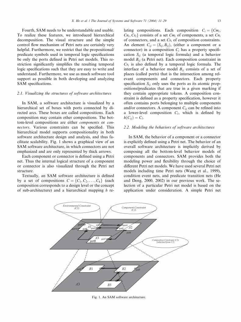
In SAM, a software architecture is visualized by a

hierarchical set of boxes with ports connected by di-

rected arcs. These boxes are called compositions. Each

composition may contain other compositions. The bot-

tom-level compositions are either components or con-

nectors. Various constraints can be specified. This

hierarchical model supports compositionality in bothsoftware architecture design and analysis, and thus fa-

cilitate scalability. Fig. 1 shows a graphical view of an

SAM software architecture, in which connectors are not

emphasized and are only represented by thick arrows.

Each component or connector is defined using a Petri

net. Thus the internal logical structure of a component

or connector is also visualized through the Petri net

structure.Textually, an SAM software architecture is defined

by a set of compositions C ¼ fC1;C2; . . . ;Ckg (each

composition corresponds to a design level or the concept

of sub-architecture) and a hierarchical mapping h re-

Fig. 1. An SAM softw

lating compositions. Each composition Ci ¼ fCmi;Cni;Csig consists of a set Cmi of components, a set Cniof connectors, and a set Csi of composition constraints.

An element Cij ¼ ðSij;BijÞ, (either a component or a

connector) in a composition Ci has a property specifi-

cation Sij (a temporal logic formula) and a behaviormodel Bij (a Petri net). Each composition constraint in

Csi is also defined by a temporal logic formula. The

interface of a behavior model Bij consists of a set of

places (called ports) that is the intersection among rel-

evant components and connectors. Each property

specification Sij only uses the ports as its atomic prop-

ositions/predicates that are true in a given marking if

they contain appropriate tokens. A composition con-straint is defined as a property specification, however it

often contains ports belonging to multiple components

and/or connectors. A component Cij can be refined into

a lower-level composition Cl, which is defined by

hðCijÞ ¼ Cl.

2.2. Modeling the behaviors of software architectures

In SAM, the behavior of a component or a connector

is explicitly defined using a Petri net. The behavior of an

overall software architecture is implicitly derived by

composing all the bottom-level behavior models of

components and connectors. SAM provides both the

modeling power and flexibility through the choice of

different Petri net models. We have used several Petri net

models including time Petri nets (Wang et al., 1999),condition event nets, and predicate transition nets (He

and Deng, 2000, 2002) in our previous work. The se-

lection of a particular Petri net model is based on the

application under consideration. A simple Petri net

are architecture.

�14 X. He et al. / The Journal of Systems and Software 71 (2004) 11–29

model such as condition event nets is adequate when we

only need to deal with simple control flows and data-

independent constraints; while a more powerful Petri net

model such as predicate transition nets is needed to

handle both control and data. To study performance

related constraints, a more specialized Petri net modelsuch as stochastic Petri nets is more appropriate and

convenient. In this paper, we use predicate transition

nets (PrT nets), by Genrich and Lautenbach (1981) to

model behaviors.

In the following sections, we give a brief definition of

PrT nets using the conventions in (He, 1996).

2.2.1. The syntax and static semantics of PrT nets

A PrT net is a tuple (N, Spec, ins) where

(1) N ¼ ðP ; T ; F Þ is the net structure, in which

(i) P and T are non-empty finite sets satisfying

P \ T ¼£ (P and T are the sets of places and tran-

sitions of N, respectively),

(ii) F � ðP � T Þ [ ðT � P Þ is a flow relation (the arcs

of N);(2) Spec ¼ ðS;OP ;EqÞ is the underlying specification,

and consists of a signature S ¼ ðS;OP Þ and a set

Eq of S-equations. Signature S ¼ ðS;OPÞ includesa set of sorts S and a family OP ¼ ðOPs1;...;sn;sÞ ofsorted operations for s1; . . . ; sn, s 2 S. For each

s 2 S, we use CONs to denote OP;s (the 0-ary opera-

tion of sort s), i.e. the set of constant symbols of sort

s. The S-equations in Eq define the meanings andproperties of operations in OP. We often simply

use familiar operations and their properties without

explicitly listing the relevant equations. Spec is a

meta-language to define the tokens, labels, and con-

straints of a PrT net. Tokens of a PrT net are ground

terms of the signature S, written MCONS. The set of

labels is denoted using LabelSðX Þ (X is the set of

sorted variables disjoint with OP). Each label canbe a multiple set expression of the form fk1x1; . . . ;knxng. Constraints of a PrT net are a subset of first

order logic formulas (where the domains of quanti-

fiers are finite and any free variable in a constraint

appears in the label of some connecting arc of the

transition), and thus are essentially propositional

logic formulas. The subset of first order logical for-

mulas contains the S-terms of sort bool over X, de-noted as TermOP ;boolðX Þ.

(3) ins ¼ ðu; L;R;M0Þ is a net inscription that associ-

ates a net element in N with its denotation in

Spec:

(i) u : P ! }ðSÞ is the data definition of N and

associates each place p in P with a subset of sorts

in S.

(ii) L : F ! LabelSðX Þ is a sort-respecting labeling ofPrT net. We use the following abbreviation in the

following definitions:

Lðx; yÞ ¼ Lðx; yÞ iff ðx; yÞ 2 F£ otherwise

(iii) R : T ! TermOP ;boolðX Þ is a well-defined con-

straining mapping, which associates each transi-

tion t in T with a first order logic formula

defined in the underlying algebraic specification.

Furthermore, the constraint of a transition defines

the meaning of the transition.

(iv) M0 : P ! MCONS is a sort-respecting initialmarking. The initial marking assigns a multi-set

of tokens to each place p in P.

2.2.2. Dynamic semantics of PrT nets

(1) Markings of a PrT net N are mappings M : P !MCONS ;

(2) An occurrence mode of N is a substitution

a ¼ fx1 c1; . . . ; xn cng, which instantiatestyped label variables. We use e: a to denote the result

of instantiating an expression e with a, in which e

can be either a label expression or a constraint;

(3) Given a marking M, a transition t 2 T , and an oc-

currence mode a, t is a_enabled at M iff the follow-

ing predicate is true: 8p : p 2 P . (�Lðp; tÞ : aÞ �MðpÞÞ ^ RðtÞ : a;

(4) If tis a_enabled at M, t may fire in occurrence modea. The firing of t with a returns the marking M 0 de-fined by M 0ðpÞ ¼ MðpÞ � �Lðp; tÞ : a [ �Lðt; pÞ : a for

p 2 P . We useM ½t=aiM 0 to denote the firing of t with

occurrence a under marking M. As in traditional Pe-

tri nets, two enabled transitions may fire at the same

time as long as they are not in conflict;

(5) For a marking M, the set ½Mi of markings reachable

from M is the smallest set of markings such thatM 2 ½Mi and if M 0 2 ½Mi and M 0½t=aiM 00 then

M 00 2 ½Mi, for some t 2 T and occurrence mode a(note: concurrent transition firings do not produce

additional new reachable markings);

(6) An execution sequence (or a run) M0T0M1T1 . . . of Nis either finite when the last marking is terminal (no

more enabled transition in the last marking) or infi-

nite, in which each Ti is an execution step consistingof a set of non-conflict firing transitions;

(7) The behavior of N (denoted by compðNÞ) is the set ofall execution sequences starting from the initial

marking.

The dining philosophers problem is a classic multi-

process synchronization problem introduced by Dijk-

stra. The problem consists of k philosophers sitting at around table who do nothing but think and eat. Between

each philosopher, there is a single chopstick. In order to

eat, a philosopher must have both chopsticks. A prob-

lem can arise if each philosopher grabs the chopstick on

the right, then waits for the chopstick on the left. In this

case a deadlock has occurred. The challenge in the


dining philosophers problem is to design a protocol so

that the philosophers do not deadlock (i.e. the entire set

of philosophers does not stop and wait indefinitely), and

so that no philosopher starves (i.e. every philosopher

eventually gets his/her hands on a pair of chopsticks).

The following is an example of the PrT net model of thedining philosophers problem.

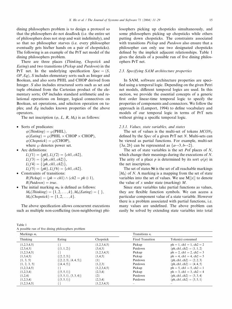
There are three places (Thinking, Chopstick and

Eating) and two transitions (Pickup and Putdown) in the

PrT net. In the underlying specification Spec ¼ ðS;OP ;EqÞ, S includes elementary sorts such as Integer and

Boolean, and also sorts PHIL and CHOP derived from

Integer. S also includes structured sorts such as set and

tuple obtained from the Cartesian product of the ele-mentary sorts; OP includes standard arithmetic and re-

lational operations on Integer, logical connectives on

Boolean, set operations, and selection operation on tu-

ples; and Eq includes known properties of the above

operators.

The net inscription (u, L, R, M0) is as follows:

• Sorts of predicates:uðThinkingÞ ¼ }ðPHILÞ;uðEatingÞ ¼ }ðPHIL� CHOP� CHOPÞ,uðChopstickÞ ¼ }ðCHOPÞ,where } denotes power set.

• Arc definitions:

Lðf 1Þ ¼ fphg; Lðf 2Þ ¼ fch1; ch2g;Lðf 3Þ ¼ fhph; ch1; ch2ig,Lðf 4Þ ¼ fhph; ch1; ch2ig;Lðf 5Þ ¼ fphg; Lðf 6Þ ¼ fch1; ch2g.

• Constraints of transitions:

RðPickupÞ ¼ ðph ¼ ch1Þ ^ ðch2 ¼ ph� 1Þ;RðPutdownÞ ¼ true.

• The initial marking m0 is defined as follows:

M0ðThinkingÞ ¼ f1; 2; . . . ; kg;M0ðEatingÞ ¼ f g;M0ðChopstickÞ ¼ f1; 2; . . . ; kg.

The above specification allows concurrent executions

such as multiple non-conflicting (non-neighboring) phi-

Table 1

A possible run of five dining philosophers problem

Markings mi

Thinking Eating Chopstick

{1,2,3,4,5} { } {1,2,3,4,5}

{2,3,4,5} fh1; 1; 2ig {3,4,5}

{1,2,3,4,5} { } {1,2,3,4,5}

{1,3,4,5} fh2; 2; 3ig {1,4,5}

{1, 3, 5} fh2; 2; 3i; h4; 4; 5ig {1}

{1, 2, 3, 5} fh4; 4; 5ig {1,2,3}

{1,2,3,4,5} { } {1,2,3,4,5}

{1,2,3,4} fh5; 5; 1ig {2,3,4}

{1,2,4} fh5; 5; 1i; h3; 3; 4ig {2}

{1,2,3,4} fh5; 5; 1ig {2,3,4}

{1,2,3,4,5} { } {1,2,3,4,5}

losophers picking up chopsticks simultaneously, and

some philosophers picking up chopsticks while others

putting down chopsticks. The constraints associated

with transitions Pickup and Putdown also ensure that a

philosopher can only use two designated chopsticks

defined by the implicit adjacent relationships. Table 1gives the details of a possible run of five dining philos-

ophers PrT net.

2.3. Specifying SAM architecture properties

In SAM, software architecture properties are speci-

fied using a temporal logic. Depending on the given Petri

net models, different temporal logics are used. In thissection, we provide the essential concepts of a generic

first order linear-time temporal logic to specify the

properties of components and connectors. We follow the

approach in (Lamport, 1994) to define vocabulary and

models of our temporal logic in terms of PrT nets

without giving a specific temporal logic.

2.3.1. Values, state variables, and states

The set of values is the multi-set of tokens MCONS

defined by the Spec of a given PrT net N. Multi-sets can

be viewed as partial functions. For example, multi-set

f3a; 2bg can be represented as fa 7!3; b 7!2g.The set of state variables is the set Pof places of N,

which change their meanings during the executions of N.

The arity of a place p is determined by its sort uðpÞ inthe net inscription.

The set of states St is the set of all reachable markings

½M0i of N. A marking is a mapping from the set of state

variables into the set of values. We use M½jxj� to denote

the value of x under state (marking) M.

Since state variables take partial functions as values,

they are flexible function symbols. We can access a

particular component value of a state variable. However

there is a problem associated with partial functions, i.e.many values are undefined. The above problem can

easily be solved by extending state variables into total

Transitions ni

Fired Transition Token(s) consumed

Pickup ph ¼ 1, ch1 ¼ 1, ch2 ¼ 2

Putdown hph; ch1; ch2i ¼ h1; 1; 2iPickup ph ¼ 2, ch1 ¼ 2, ch2 ¼ 3

Pickup ph ¼ 4, ch1 ¼ 4, ch2 ¼ 5

Putdown hph; ch1; ch2i ¼ h2; 2; 3iPutdown hph; ch1; ch2i ¼ h4; 4; 5iPickup ph ¼ 5, ch1 ¼ 5, ch2 ¼ 1

Pickup ph ¼ 3, ch1 ¼ 3, ch2 ¼ 4

Putdown hph; ch1; ch2i ¼ h3; 3; 4iPutdown hph; ch1; ch2i ¼ h5; 5; 1i– –


functions in the following way: for any n-ary state

variable p , any tuple c 2 MCONnS and any state M, if

pðcÞ is undefined under M, then let M ½jpðcÞj� ¼ 0. The

above extension is consistent with the semantics of PrT

nets. Furthermore we can consider the meaning ½jpðcÞj�of the function application pðcÞ as a mapping fromstates to Nat using a postfix notation for function ap-

plication M ½jpðcÞj�.

2.3.2. Rigid variables, rigid function and predicate sym-

bols

Rigid variables are individual variables that do not

change their meanings during the executions of N. All

rigid variables occurring in our temporal logic formulasare bound (quantified), and they are the only variables

that can be quantified. Rigid variables are variables

appearing in the label expressions and constraints of N.

Rigid function and predicate symbols do not change

their meanings during the executions of N. The set of

rigid function and predicate symbols is defined in the

Spec of N.

2.3.3. State functions, predicates, and transitions

A state function is an expression built from values,

state variables, rigid function and predicate symbols.

For example ½jpðcÞ þ 1j� is a state function where c and 1

are values, p is a state variable, + is a rigid function

symbol. Since the meanings of rigid symbols are not

affected by any state, thus for any given state M,

M ½jpðcÞ þ 1j� ¼ M ½jpðcÞj� þ 1.A predicate is a boolean-valued state function. A

predicate p is said to be satisfied by a state M iff M ½jpj� istrue.

A transition is a particular kind of predicates that

contain primed state variables, e.g. ½jp0ðcÞ ¼ pðcÞ þ 1j�.A transition relates two states (an old state and a new

state), where the unprimed state variables refer to the

old state and the primed state variables refer to the newstate. Therefore the meaning of a transition is a relation

between states. The term transition used here is a tem-

poral logic entity. Although it reflects the nature of a

transition in a PrT net N, it is not a transition in N. For

example, given a pair of states M and M 0 : M ½jp0ðcÞ ¼pðcÞ þ 1j�M 0 is defined by M 0½jp0ðcÞj� ¼ M ½jpðcÞj� þ 1.

Given a transition t, a pair of states M and M 0 is calleda ‘‘transition step’’ iff M ½jtj�M 0 equals true. We caneasily generalize any predicate p without primed state

variables into a relation between states by replacing all

unprimed state variables with their primed versions

such that M ½jp0j�M 0 equals M 0½jpj� for any states M and

M 0.

2.3.4. Temporal formulas

Temporal formulas are built from elementary for-mulas (predicates and transitions) using logical con-

nectives : and ^ (and derived logical connectives _, ),

and () ), universal quantifier 8 and derived existential

quantifier 9, and temporal operators always �, some-

times �, and until U.

The semantics of temporal logic is defined on be-

haviors (infinite sequences of states). The behaviors are

obtained from the execution sequences of PrT netswhere the last marking of a finite execution sequence is

repeated infinitely many times at the end of the execu-

tion sequence. For example, for an execution sequence

M0; . . . ;Mn, the following behavior r ¼ hhM0; . . . ;Mn;Mn; . . .ii is obtained. We denote the set of all pos-

sible behaviors obtained from a given PrT net as St1.Let u and v be two arbitrary temporal formulas, p be

an n-ary predicate, t be a transition, x; x1; . . . ; xn be rigidvariables, r ¼ hhM0;M1; . . .ii be a behavior, and

rk ¼ hhMk;Mkþ1; . . .ii be a k step shifted behavior se-

quence; we define the semantics of temporal formulas

recursively as follows:

(1) r½jpðx1; . . . ; xnÞj� � M0½jpðx1; . . . ; xnÞj�(2) r½jtj� � M0½jtj�M1

(3) r½j:uj� � :r½juj�(4) r½ju ^ vj� � r½juj� ^ r½jvj�(5) r½j8xuj� � 8xr½juj�(6) r½j�uj� � 8n 2 Natrn½juj�(7) r½juUvj� � 9krk½jvj� ^ 806 n < krn½juj�

A temporal formula u is said to be satisfiable, denoted

as rj ¼ u, iff there is an execution r such that r½juj� istrue, i.e. rj ¼ u() 9r 2 St1. r½juj�. u is validwith re-gard to N, denoted as N j ¼ u, iff it is satisfied by all

possible behaviors St1 from N : N j ¼ u() 8r 2St1r½juj�.

2.3.5. Defining system properties in temporal logic

Specifying architecture properties in SAM becomes

defining PrT net properties using temporal logic. Ca-

nonical forms for a variety of system properties such assafety, guarantee, obligation, response, persistence, and

reactivity are given in (Manna and Pnueli, 1992). For

example, the following temporal logic formulas specify a

safety property and a liveness property of the PrT net in

Fig. 2, respectively:

• Mutual exclusion: 8ph 2 f1; . . . ; kg�: ðhph; ; i 2Eating ^ hph� 1; ; i 2 EatingÞ which defines that noadjacent philosophers can eat at the same time.

• Starvation freedom: 8ph2f1;...;kg}ðhph; ; i2EatingÞwhich states that every philosopher will eventually get

a chance to eat.

2.4. Analyzing SAM architecture specifications

An SAM architectural specification is well-defined ifthe ports of a component are preserved (contained) in

the set of exterior ports of its refinement and the prop-

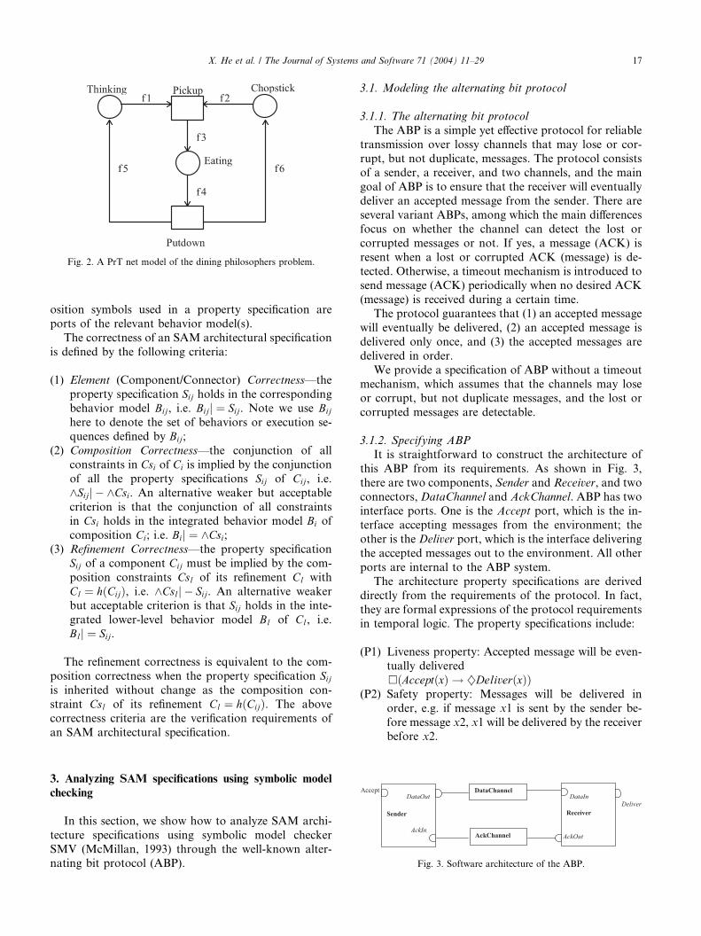
Fig. 2. A PrT net model of the dining philosophers problem.


osition symbols used in a property specification are

ports of the relevant behavior model(s).

The correctness of an SAM architectural specification

is defined by the following criteria:

(1) Element (Component/Connector) Correctness––the

property specification Sij holds in the correspondingbehavior model Bij, i.e. Bijj ¼ Sij. Note we use Bij

here to denote the set of behaviors or execution se-

quences defined by Bij;

(2) Composition Correctness––the conjunction of all

constraints in Csi of Ci is implied by the conjunction

of all the property specifications Sij of Cij, i.e.

^Sijj � ^Csi. An alternative weaker but acceptable

criterion is that the conjunction of all constraintsin Csi holds in the integrated behavior model Bi of

composition Ci; i.e. Bij ¼ ^Csi;(3) Refinement Correctness––the property specification

Sij of a component Cij must be implied by the com-

position constraints Csl of its refinement Cl with

Cl ¼ hðCijÞ, i.e. ^Cslj � Sij. An alternative weaker

but acceptable criterion is that Sij holds in the inte-

grated lower-level behavior model Bl of Cl, i.e.Blj ¼ Sij.

The refinement correctness is equivalent to the com-

position correctness when the property specification Sijis inherited without change as the composition con-

straint Csl of its refinement Cl ¼ hðCijÞ. The above

correctness criteria are the verification requirements of

an SAM architectural specification.

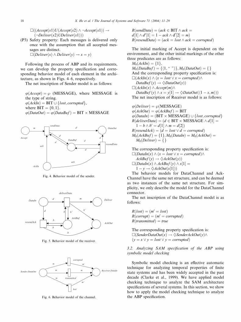
Fig. 3. Software architecture of the ABP.

3. Analyzing SAM specifications using symbolic model

checking

In this section, we show how to analyze SAM archi-

tecture specifications using symbolic model checker

SMV (McMillan, 1993) through the well-known alter-nating bit protocol (ABP).

3.1. Modeling the alternating bit protocol

3.1.1. The alternating bit protocol

The ABP is a simple yet effective protocol for reliable

transmission over lossy channels that may lose or cor-

rupt, but not duplicate, messages. The protocol consistsof a sender, a receiver, and two channels, and the main

goal of ABP is to ensure that the receiver will eventually

deliver an accepted message from the sender. There are

several variant ABPs, among which the main differences

focus on whether the channel can detect the lost or

corrupted messages or not. If yes, a message (ACK) is

resent when a lost or corrupted ACK (message) is de-

tected. Otherwise, a timeout mechanism is introduced tosend message (ACK) periodically when no desired ACK

(message) is received during a certain time.

The protocol guarantees that (1) an accepted message

will eventually be delivered, (2) an accepted message is

delivered only once, and (3) the accepted messages are

delivered in order.

We provide a specification of ABP without a timeout

mechanism, which assumes that the channels may loseor corrupt, but not duplicate messages, and the lost or

corrupted messages are detectable.

3.1.2. Specifying ABP

It is straightforward to construct the architecture of

this ABP from its requirements. As shown in Fig. 3,

there are two components, Sender and Receiver, and two

connectors, DataChannel and AckChannel. ABP has twointerface ports. One is the Accept port, which is the in-

terface accepting messages from the environment; the

other is the Deliver port, which is the interface delivering

the accepted messages out to the environment. All other

ports are internal to the ABP system.

The architecture property specifications are derived

directly from the requirements of the protocol. In fact,

they are formal expressions of the protocol requirementsin temporal logic. The property specifications include:

(P1) Liveness property: Accepted message will be even-

tually delivered

�ðAcceptðxÞ ! }DeliverðxÞÞ(P2) Safety property: Messages will be delivered in

order, e.g. if message x1 is sent by the sender be-

fore message x2, x1 will be delivered by the receiverbefore x2.


�ððAcceptðx1ÞUðAcceptðx2Þ ^ :Acceptðx1ÞÞ !ð:Deliverðx2ÞUDeliverðx1ÞÞÞ

(P3) Safety property: Each messages is delivered only

once with the assumption that all accepted mes-

sages are distinct.

�ðDeliverðxÞ ^ DeliverðyÞ ! x ¼ yÞ

Following the process of ABP and its requirements,

we can develop the property specification and corre-

sponding behavior model of each element in the archi-

tecture, as shown in Figs. 4–6, respectively.

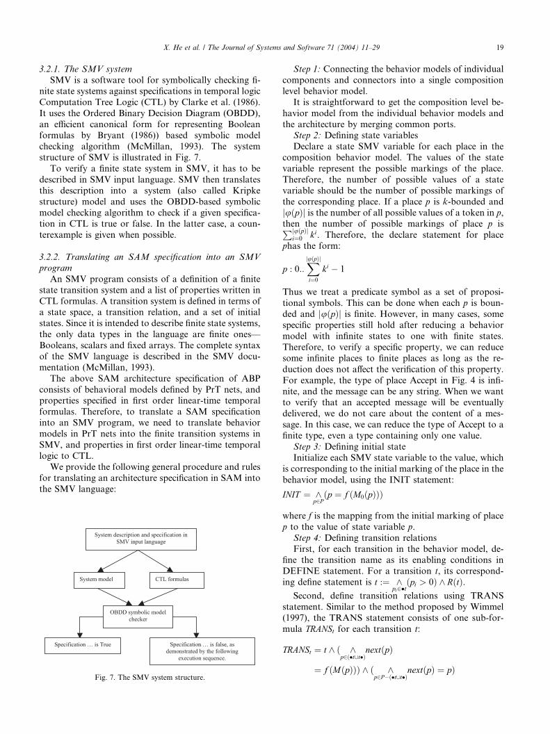
The net inscription of Sender model is as follows:

uðAcceptÞ ¼ } (MESSAGE), where MESSAGE isthe type of string.

uðAckInÞ ¼ BIT [ flost; corruptedg,where BIT ¼ f0; 1g.uðDataOutÞ ¼ uðDataBuf Þ ¼ BIT�MESSAGE

Fig. 4. Behavior model of the sender.

Fig. 5. Behavior model of the receiver.

Fig. 6. Behavior model of the channel.

RðsendDataÞ ¼ ðack 2 BIT ^ ack ¼d½1� ^ d 0½1� ¼ 1� ack ^ d0½2� ¼ mÞRðresendDataÞ ¼ ðack ¼ lost ^ ack ¼ corruptedÞ

The initial marking of Accept is dependent on theenvironment, and the other initial markings of the other

three predicates are as follows:

M0ðAckInÞ ¼ f1g;M0ðDataBuf Þ ¼ fh1; \ "ig;M0ðDataOutÞ ¼ fgAnd the corresponding property specification is:

�ðAckInðxÞ ^ ðx ¼ lost _ x ¼ corruptedÞ^DataBuf ðyÞ ! }DataOutðyÞÞ

�ðAckInðxÞ ^ AcceptðmÞ^DataBuf ðyÞ ^ x ¼ y½1� ! }DataOutðh1� x;miÞÞ

The net inscription of Receiver model is as follows:

uðDeliverÞ ¼ }ðMESSAGEÞuðAckOutÞ ¼ uðAckBuf Þ ¼ BIT

uðDataInÞ ¼ ðBIT�MESSAGEÞ [ flost; corruptedgRðdeliverDataÞ ¼ ðd 2 BIT�MESSAGE ^ d½1� ¼

1� b ^ b0 ¼ d½1� ^ m ¼ d½2�ÞRðresendAckÞ ¼ ðd ¼ lost _ d ¼ corruptedÞM0ðAckBuf Þ ¼ f1g;M0ðDataInÞ ¼ M0ðAckOutÞ ¼

M0ðDeliverÞ ¼ fg

The corresponding property specification is:�ðDataInðxÞ ^ ðx ¼ lost _ x ¼ corruptedÞ^

AckBuf ðyÞ ! }AckOutðyÞÞ�ðDataInðxÞ ^ AckBuf ðyÞ ^ x½1� ¼

1� y ! }AckOutðx½1�ÞÞThe behavior models for DataChannel and Ack-

Channel have the same net structure, and can be deemed

as two instances of the same net structure. For sim-

plicity, we only describe the model for the DataChannelconnector.

The net inscription of the DataChannel model is as

follows:

RðlostÞ ¼ ðm0 ¼ lostÞRðcorruptÞ ¼ ðm0 ¼ corruptedÞRðtransmittedÞ ¼ true

The corresponding property specification is:

�ðSenderDataOutðxÞ ! }SenderAckOutðyÞ^ðy ¼ x _ y ¼ lost _ y ¼ corruptedÞ

3.2. Analyzing SAM specification of the ABP using

symbolic model checking

Symbolic model checking is an effective automatic

technique for analyzing temporal properties of finite

state systems and has been widely accepted in the past

decade (Clarke et al., 1999). We have applied model

checking technique to analyze the SAM architecture

specifications of several systems. In this section, we show

how to apply the model checking technique to analyzethe ABP specification.


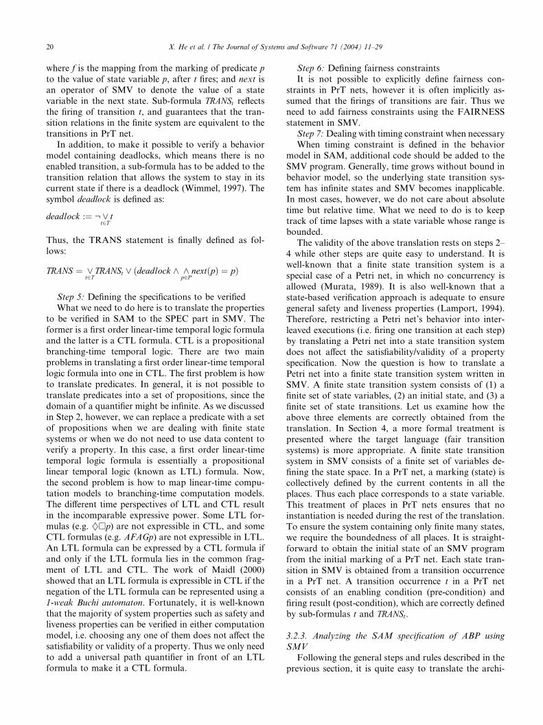
3.2.1. The SMV system

SMV is a software tool for symbolically checking fi-

nite state systems against specifications in temporal logic

Computation Tree Logic (CTL) by Clarke et al. (1986).

It uses the Ordered Binary Decision Diagram (OBDD),

an efficient canonical form for representing Booleanformulas by Bryant (1986)) based symbolic model

checking algorithm (McMillan, 1993). The system

structure of SMV is illustrated in Fig. 7.

To verify a finite state system in SMV, it has to be

described in SMV input language. SMV then translates

this description into a system (also called Kripke

structure) model and uses the OBDD-based symbolic

model checking algorithm to check if a given specifica-tion in CTL is true or false. In the latter case, a coun-

terexample is given when possible.

3.2.2. Translating an SAM specification into an SMV

program

An SMV program consists of a definition of a finite

state transition system and a list of properties written in

CTL formulas. A transition system is defined in terms ofa state space, a transition relation, and a set of initial

states. Since it is intended to describe finite state systems,

the only data types in the language are finite ones––

Booleans, scalars and fixed arrays. The complete syntax

of the SMV language is described in the SMV docu-

mentation (McMillan, 1993).

The above SAM architecture specification of ABP

consists of behavioral models defined by PrT nets, andproperties specified in first order linear-time temporal

formulas. Therefore, to translate a SAM specification

into an SMV program, we need to translate behavior

models in PrT nets into the finite transition systems in

SMV, and properties in first order linear-time temporal

logic to CTL.

We provide the following general procedure and rules

for translating an architecture specification in SAM intothe SMV language:

Fig. 7. The SMV system structure.

Step 1: Connecting the behavior models of individual

components and connectors into a single composition

level behavior model.

It is straightforward to get the composition level be-

havior model from the individual behavior models and

the architecture by merging common ports.Step 2: Defining state variables

Declare a state SMV variable for each place in the

composition behavior model. The values of the state

variable represent the possible markings of the place.

Therefore, the number of possible values of a state

variable should be the number of possible markings of

the corresponding place. If a place p is k-bounded and

juðpÞj is the number of all possible values of a token in p,then the number of possible markings of place p isP uðpÞj j

i¼0 ki. Therefore, the declare statement for place

phas the form:

p : 0::XuðpÞj j

i¼0ki � 1

Thus we treat a predicate symbol as a set of proposi-

tional symbols. This can be done when each p is boun-ded and juðpÞj is finite. However, in many cases, some

specific properties still hold after reducing a behavior

model with infinite states to one with finite states.

Therefore, to verify a specific property, we can reduce

some infinite places to finite places as long as the re-

duction does not affect the verification of this property.

For example, the type of place Accept in Fig. 4 is infi-

nite, and the message can be any string. When we wantto verify that an accepted message will be eventually

delivered, we do not care about the content of a mes-

sage. In this case, we can reduce the type of Accept to a

finite type, even a type containing only one value.

Step 3: Defining initial state

Initialize each SMV state variable to the value, which

is corresponding to the initial marking of the place in the

behavior model, using the INIT statement:

INIT ¼p̂2Pðp ¼ f ðM0ðpÞÞÞ

where f is the mapping from the initial marking of place

p to the value of state variable p.

Step 4: Defining transition relations

First, for each transition in the behavior model, de-fine the transition name as its enabling conditions in

DEFINE statement. For a transition t, its correspond-

ing define statement is t :¼ ^pi2�tðpi > 0Þ ^ RðtÞ.

Second, define transition relations using TRANS

statement. Similar to the method proposed by Wimmel

(1997), the TRANS statement consists of one sub-for-

mula TRANSt for each transition t:

TRANSt ¼ t ^ ð ^p2ð�t[t�Þ

nextðpÞ

¼ f ðMðpÞÞÞ ^ ð ^p2P�ð�t[t�Þ

nextðpÞ ¼ pÞ


where f is the mapping from the marking of predicate p

to the value of state variable p, after t fires; and next is

an operator of SMV to denote the value of a state

variable in the next state. Sub-formula TRANSt reflectsthe firing of transition t, and guarantees that the tran-

sition relations in the finite system are equivalent to thetransitions in PrT net.

In addition, to make it possible to verify a behavior

model containing deadlocks, which means there is no

enabled transition, a sub-formula has to be added to the

transition relation that allows the system to stay in its

current state if there is a deadlock (Wimmel, 1997). The

symbol deadlock is defined as:

deadlock :¼ :_t2T

t

Thus, the TRANS statement is finally defined as fol-

lows:

TRANS ¼ _t2T

TRANSt _ ðdeadlock ^p̂2P

nextðpÞ ¼ pÞ

Step 5: Defining the specifications to be verified

What we need to do here is to translate the properties

to be verified in SAM to the SPEC part in SMV. The

former is a first order linear-time temporal logic formula

and the latter is a CTL formula. CTL is a propositional

branching-time temporal logic. There are two mainproblems in translating a first order linear-time temporal

logic formula into one in CTL. The first problem is how

to translate predicates. In general, it is not possible to

translate predicates into a set of propositions, since the

domain of a quantifier might be infinite. As we discussed

in Step 2, however, we can replace a predicate with a set

of propositions when we are dealing with finite state

systems or when we do not need to use data content toverify a property. In this case, a first order linear-time

temporal logic formula is essentially a propositional

linear temporal logic (known as LTL) formula. Now,

the second problem is how to map linear-time compu-

tation models to branching-time computation models.

The different time perspectives of LTL and CTL result

in the incomparable expressive power. Some LTL for-

mulas (e.g. }�p) are not expressible in CTL, and someCTL formulas (e.g. AFAGp) are not expressible in LTL.

An LTL formula can be expressed by a CTL formula if

and only if the LTL formula lies in the common frag-

ment of LTL and CTL. The work of Maidl (2000)

showed that an LTL formula is expressible in CTL if the

negation of the LTL formula can be represented using a

1-weak Buchi automaton. Fortunately, it is well-known

that the majority of system properties such as safety andliveness properties can be verified in either computation

model, i.e. choosing any one of them does not affect the

satisfiability or validity of a property. Thus we only need

to add a universal path quantifier in front of an LTL

formula to make it a CTL formula.

Step 6: Defining fairness constraints

It is not possible to explicitly define fairness con-

straints in PrT nets, however it is often implicitly as-

sumed that the firings of transitions are fair. Thus we

need to add fairness constraints using the FAIRNESS

statement in SMV.Step 7:Dealing with timing constraint when necessary

When timing constraint is defined in the behavior

model in SAM, additional code should be added to the

SMV program. Generally, time grows without bound in

behavior model, so the underlying state transition sys-

tem has infinite states and SMV becomes inapplicable.

In most cases, however, we do not care about absolute

time but relative time. What we need to do is to keeptrack of time lapses with a state variable whose range is

bounded.

The validity of the above translation rests on steps 2–

4 while other steps are quite easy to understand. It is

well-known that a finite state transition system is a

special case of a Petri net, in which no concurrency is

allowed (Murata, 1989). It is also well-known that a

state-based verification approach is adequate to ensuregeneral safety and liveness properties (Lamport, 1994).

Therefore, restricting a Petri net’s behavior into inter-

leaved executions (i.e. firing one transition at each step)

by translating a Petri net into a state transition system

does not affect the satisfiability/validity of a property

specification. Now the question is how to translate a

Petri net into a finite state transition system written in

SMV. A finite state transition system consists of (1) afinite set of state variables, (2) an initial state, and (3) a

finite set of state transitions. Let us examine how the

above three elements are correctly obtained from the

translation. In Section 4, a more formal treatment is

presented where the target language (fair transition

systems) is more appropriate. A finite state transition

system in SMV consists of a finite set of variables de-

fining the state space. In a PrT net, a marking (state) iscollectively defined by the current contents in all the

places. Thus each place corresponds to a state variable.

This treatment of places in PrT nets ensures that no

instantiation is needed during the rest of the translation.

To ensure the system containing only finite many states,

we require the boundedness of all places. It is straight-

forward to obtain the initial state of an SMV program

from the initial marking of a PrT net. Each state tran-sition in SMV is obtained from a transition occurrence

in a PrT net. A transition occurrence t in a PrT net

consists of an enabling condition (pre-condition) and

firing result (post-condition), which are correctly defined

by sub-formulas t and TRANSt.

3.2.3. Analyzing the SAM specification of ABP using

SMV

Following the general steps and rules described in the

previous section, it is quite easy to translate the archi-


tecture specification to SMV program. The complete

SMV program for ABP without timer is shown in Ap-

pendix A.

Our goal is to verify that the compositional archi-

tecture specification satisfies the three properties, (P1),

(P2) and (P3) described in Section 3.1.2. To make theunderlying transition system finite and to simplify the

analysis, we assume that there are eight distinct mes-

sages accepted initially. Namely, there are eight distinct

tokens in place Accept. The ids for the messages range

from 1 to 8. The messages sent by the Sender are in the

order from 8 to 1. No any other message is accepted. We

verify that all eight messages and only eight messages

are delivered, and eight messages are delivered in theorder they are sent by the Sender.

With the above assumption, we translate the archi-

tecture specification to the SMV program as follows.

Since juðAckBuf Þj ¼ 2 and it is 1-bounded, we can

define the state variable AckBuf as: AckBuf: 0 . . . 2;However, to make it more meaningful, we define it as

follows instead: AckBuf {0, bit0, bit1}; where state 0

means there is no token in Place AckBuf. Similarly, wecan define AckOut and AckIn. AckOut: {0, bit0, bit1}

and AckIn: {0, bit0, bit1, lost, corrupted}, respectively.

We have noted from the assumption that

juðAcceptÞj ¼ 8 and it is eight-bounded, so it seems that

we should define Accept to range between 0 andP8i¼0 8

i � 1. In fact, Accept can be represented by eight

values (in addition to 0) since messages are sent in order.

So we define Accept as: Accept: 0 . . . 8; where state 0

means there is no token in Place Accept, i (i > 0) means

that there are i tokens in Accept and the id for each

message is 1 to i, respectively. Similarly, Deliver is de-

fined as: Deliver: 0 . . . 8.To make it more convenient to extract message id and

associated bit tag, we define the remaining two variables

as follows:

DataBuf : 0 . . . 17; ==0 : empty; 1 :==undefined; 2–17 : message id� 2þ bit

DataOut : 0 . . . 17;DataIn : 0 . . . 19; ==18-lost; 19-corrupted

After the state variables are defined, the initial state

and transition relations are defined straightforwardly.

See Appendix A for the complete SMV program for this

model.The SPEC part is defined as follows according to the

properties we intend to verify.

(1) All messages are eventually delivered. This formula

ensures property (P1).

AF Deliver ¼ 8

where A is the universal path quantifier and F is the

temporal operator } in CTL.

(2) Messages are delivered in order and all delivered

message are distinct. This formula ensures proper-

ties (P2) and (P3).

AGðdeliverData & !next ðdeliverDataÞ ! DataIn=2

¼ Deliver þ 1Þ;

where G is the temporal operator � in CTL.

If we run the SMV program now, the first formula is

false. This is because we have not considered the fairness

constraints. ABP works successfully only when thechannels do not always lose or corrupt messages.

Therefore we need to add fairness constraints in the

SMV program to make sure that a message will get

through the channel when it is sent infinitely often. The

necessary fairness constraints are as follows:

FAIRNESS

DataOut > 0! AFðDataIn > 0 & DataIn < 18ÞAckOut > 0! AFðAckIn ¼ bit0 j AckIn ¼ bit1ÞAfter the fairness constraints are added, the specifi-

cation is evaluated to be true.

4. Analyzing SAM specifications using theorem proving

Although model checking is very effective for finite

state systems, it is in general not applicable to systemswith infinite states. Depending on the underlying Petri

net and temporal logic models used in SAM, model

checking may or may not be applicable. In the previous

Section, we showed how to apply model checking to

SAM specifications. In this section, we show how to use

the more general theorem proving approach to verify

SAM specifications. We have successfully applied the

theorem proving approach in analyzing an SAM speci-fication of an electronic commerce system.

4.1. The stanford temporal prover

STeP, the Stanford Temporal Prover, is a tool for

formal verification of temporal properties of reactive

systems (Manna et al., 1994). Fig. 8 presents an overview

of the STeP system. The main inputs are a reactive sys-tem in the form of a fair transition system (FTS) and a

property in first order linear-time temporal logic to be

proven. Verification can be performed by the model

checker or by deductive means. Model checking is au-

tomatic; deductive verification is to a large extend au-

tomatic for simple safety properties, while progress

properties require more user guidance, usually in the

form of a verification diagram. In all cases, the automaticprover is responsible for generating and proving the re-

quired verification conditions. An interactive Gentzen-

style theorem prover is used to establish those verifica-

tion conditions that cannot be proved automatically.

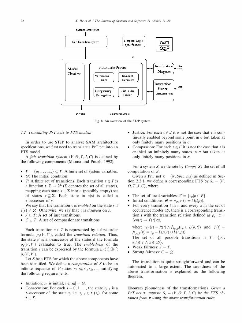
Fig. 8. An overview of the STeP system.


4.2. Translating PrT nets to FTS models

In order to use STeP to analyze SAM architecture

specifications, we first need to translate a PrT net into an

FTS model.

A fair transition system hV ;H; T ; J ;Ci is defined by

the following components (Manna and Pnueli, 1992):

• V ¼ fu1; . . . ; ung � V : A finite set of system variables.

• H: The initial condition.

• T: A finite set of transitions. Each transition s 2 T is

a function s. R! 2R (R denotes the set of all states),

mapping each state s 2 R into a (possibly empty) set

of states s � R. Each state in s(s) is called a

s-successor of s.We say that the transition s is enabled on the state s if

sðsÞ 6¼£. Otherwise, we say that s is disabled on s.

• J � T : A set of just transitions.

• C � T : A set of compassionate transitions.

Each transition s 2 T is represented by a first order

formula qsðV ; V 0Þ, called the transition relation. Thus,

the state s0 is a s-successor of the states if the formula

qsðV ; V 0Þ evaluates to true. The enabledness of thetransition s can be expressed by the formula EnðsÞ:9V 0:qsðV ; V 0Þ.

Let S be a FTS for which the above components have

been identified. We define a computation of S to be an

infinite sequence of V-states r: s0; s1; s2; . . ., satisfying

the following requirements:

• Initiation: s0 is initial, i.e. s0j ¼ H.• Consecution: For each j ¼ 0; 1; . . ., the state sjþ1 is a

s-successor of the state sj i.e. sjþ1 2 s (sj), for some

s 2 T .

• Justice: For each s 2 J it is not the case that s is con-tinually enabled beyond some point in r but taken at

only finitely many positions in r.• Compassion: For each s 2 C it is not the case that s is

enabled on infinitely many states in r but taken at

only finitely many positions in r.

For a system S, we denote by Comp( S) the set of allcomputation of S.

Given a PrT net p ¼ ðN ; Spec; InsÞ as defined in Sec-

tion 2.2.1, we define a corresponding FTS by Sp ¼ hV ;H; T ; J ;Ci, where

• The set of local variables: V ¼ fvpjp 2 Pg.• Initial conditions: H ¼ ^p2V (v ¼ M0ðpÞ).• For every transition t in p and every a in the set of

occurrence modes aS, there is a corresponding transi-

tion t with the transition relation defined as qt : a ¼ðenðtÞ ! f ðtÞÞ:a,where enðtÞ ¼ RðtÞ ^

Vp2P (vp � Lðp; tÞ) and f ðtÞ ¼V

p2P (v0p ¼ vp � Lðp; tÞ [ Lðt; pÞ).

The set of all possible transitions is T ¼ fqt :ajt 2 T ^ a 2 aSg.

• Weak fairness: J ¼ T .• Strong fairness: C ¼£.

The translation is quite straightforward and can be

automated to a large extent. The soundness of the

above transformation is explained as the followingtheorem.

Theorem (Soundness of the transformation). Given aPrT net p, suppose Sp ¼ hV ;H; T ; J ;Ci be the FTS ob-tained from p using the above transformation rules.


• For any run r ¼ m0;m1;m2; . . . 2 CompðpÞ, 8vp 2 V ,i 2 Nat, let siðvpÞ ¼ miðpÞ, then r0 ¼ s0; s1; s2; . . . 2CompðSpÞ.

• For any state sequence r ¼ s0; s1; s2; . . . 2 CompðSpÞ,8p 2 P , i 2 Nat, let miðpÞ ¼ siðvpÞ, then r0 ¼ m0;m1;m2; . . . 2 CompðpÞ.

Proof

(1) Suppose run r ¼ m0;m1;m2; . . . 2 CompðpÞ, Let thecorresponding transition sequence be t0; t1; t2; . . . ;and occurrence models be a0; a1; a2; . . . By defini-

tion, the following predicate holds:

8i 2 Nat; 8p 2 PððmiðpÞ � Lðp; tÞ : aiÞ ^ ðRðtiÞ : aiÞ^ ðmiþ1 ¼ miðpÞ � Lðp; tÞ : ai [ Lðt; pÞ : aiÞÞ

Because 8vp 2 V , s0ðvpÞ ¼ m0ðpÞ, we get s0j ¼ H. For

each i 2 Nat, (si; siþ1Þj ¼ st i;a i holds. Consequently,

s0; s1; s2 . . . is a run of Sp and the corresponding

transition sequence is st0;a0; st1;a1; st2;a2; . . . Thereforer0 ¼ s0; s1; s2; . . . 2 CompðSpÞ.

(2) Suppose r ¼ s0; s1; s2; . . . 2 CompðSpÞ. Let the corre-sponding transition sequence be st0;a0; st1;a1; st2;a2; . . .Thus mi 2 ½m0i follows from the definition ofmi and sti;ai. Consequently, r0 ¼ m0;m1;m2; . . .2 CompðpÞ. �

Reducing label substitutions: There may be many re-

dundant transitions in the resulting FTS, i.e. these

transitions never occur due to the label constrains of PrT

nets. Consequently, the label constraints can sometimes

be used to significantly reduce the number of transitions.We usually apply the label constraints to reduce transi-

tions before formal verification of the models.

To demonstrate the translation, we apply the above

rules to the dining philosophers system and obtain the

following FTS S ¼ hV ;H; T ; J ;Ci, where

V ¼ fthinking; chopstick; eatinggH ¼ ðthinking ¼ f1; 2; 3; 4; 5gÞ ^ ðeating ¼ fgÞ^ðchopstick ¼ f1; 2; 3; 4; 5gÞ

Using the label reduction strategy for occurrence

mode, we get

a S ¼ fhph; ch1; ch2i7!h1; 1; 2i,hph; ch1; ch2i7!h2; 2; 3i,htph; ch1; ch2i7!h3; 3; 4i,hph; ch1; ch2i7!h4; 4; 5i,hph; ch1; ch2i7!h5; 5; 1ig

T ¼ fqpickup : a; qputdown : aja 2 aSg,where: qpickup ¼ enðpickupÞ ! f ðpickupÞ

enðpickupÞ ¼ ðfphg � thinkingÞ^ðfch1; ch2g � chopstickÞf ðpickupÞ ¼ ðthinking0 ¼ thinking � fphgÞ^ðchopstick0 ¼ chopstick � fch1; ch2gÞ^ðeating0 ¼ eating [ fhph; ch1; ch2igÞ; and

qputdown ¼ enðputdownÞ ! f ðputdownÞ

enðputdownÞ ¼ ðfhph; ch1; ch2ig � eatingÞf ðputdownÞ ¼ ðeating0 ¼ eating � fhph; ch1; ch2igÞ^ðthinking0 ¼ thinking [ fphgÞ^ðchopstick0 ¼ chopstick [ fch1; ch2gÞ

4.3. Verifying SAM specifications using STeP

After translating a PrT net into an FTS, we can use

STeP to verify SAM architecture properties. A verifi-

cation session begins by loading a program or transition

system that describes the system of interest and entering

a temporal logic formula that expresses one or more

properties to be proved. The formula becomes the root

goal of a proof tree. There are now several ways toproceed. The most common route is to apply a verifi-

cation rule. The basic verification rule for safety prop-

erties is B-INV:

H! p; fpgT fpg�p

which states that if a property p is satisfied by the initial

conditionH, and is maintained by every transition in the

transition set T, then p holds in every state.By applying a suitable rule, a proof goal is reduced to

a few first order verification conditions or simpler tem-

poral formulas, which are usually easier to verify. The

proof is finished if all sub-goals are established. In order

to use the prover, knowledge about inference rules is

required. Furthermore, general knowledge and experi-

ence of theorem proving are essential in guiding and

obtaining successful results. STeP supports the provingof safety properties nicely; however it is in general dif-

ficult to prove liveness properties.

The FTS of the five dining philosophers problem is

described in STeP as follows:

Transition System % 5-dining philoso-

phers

out thinking:array[1 . . . 5] of bool

where Forall i:[1 . . . 5].(thinking[i]¼true)

out chopstick:array[1 . . . 5] of bool

where Forall i:[1 . . . 5].(chopstick[i]¼true)

out eating:array[1 . . . 5] of bool

where Forall i:[1. . . 5].(eating[i]¼false)

location pickup:[1 . . . 5] ! bool

location putdown:[1 . . . 5]! bool

Transition pickup[i:[1 . . . 5]] Just:

enable (thinking[i]¼true)/n chopstick[i]¼true)/n chopstick[(i mod 5)+1]¼true)

assign thinking[i] ¼ false,

chopstick[i] ¼ false,chopstick[(i mod 5)+1] ¼ false,


eating[i] ¼ true

Transition putdown[i:[1 . . . 5]] Just:

enable eating[i]¼trueassign thinking[i] ¼ true,

chopstick[i] ¼ true,

chopstick[(i mod 5)+1] ¼ true,eating[i] ¼ false

The property of mutual exclusion is specified as follows.

SPEC

variable i:[1 . . . 5]Forall i:[1 . . . 5].[](!(eating[i] ¼true /neating[(i mod 5)+1]¼true))

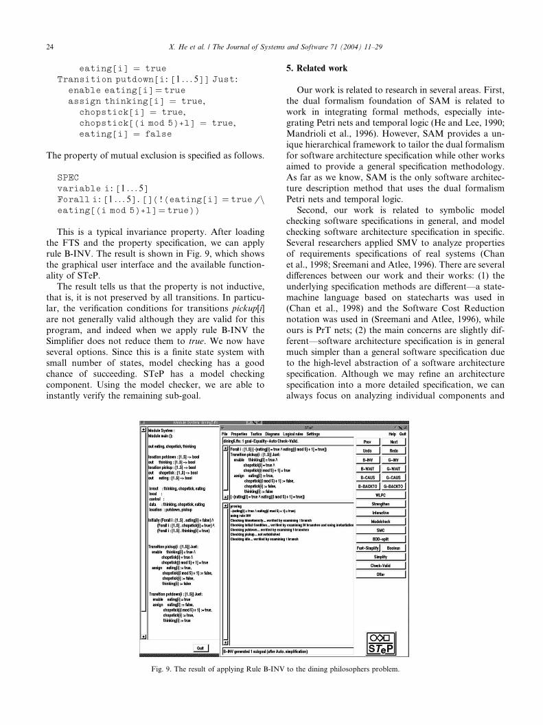
This is a typical invariance property. After loading

the FTS and the property specification, we can apply

rule B-INV. The result is shown in Fig. 9, which shows

the graphical user interface and the available function-

ality of STeP.

The result tells us that the property is not inductive,

that is, it is not preserved by all transitions. In particu-lar, the verification conditions for transitions pickup[i]are not generally valid although they are valid for this

program, and indeed when we apply rule B-INV the

Simplifier does not reduce them to true. We now have

several options. Since this is a finite state system with

small number of states, model checking has a good

chance of succeeding. STeP has a model checking

component. Using the model checker, we are able toinstantly verify the remaining sub-goal.

Fig. 9. The result of applying Rule B-INV

5. Related work

Our work is related to research in several areas. First,

the dual formalism foundation of SAM is related to

work in integrating formal methods, especially inte-

grating Petri nets and temporal logic (He and Lee, 1990;Mandrioli et al., 1996). However, SAM provides a un-

ique hierarchical framework to tailor the dual formalism

for software architecture specification while other works

aimed to provide a general specification methodology.

As far as we know, SAM is the only software architec-

ture description method that uses the dual formalism

Petri nets and temporal logic.

Second, our work is related to symbolic modelchecking software specifications in general, and model

checking software architecture specification in specific.

Several researchers applied SMV to analyze properties

of requirements specifications of real systems (Chan

et al., 1998; Sreemani and Atlee, 1996). There are several

differences between our work and their works: (1) the

underlying specification methods are different––a state-

machine language based on statecharts was used in(Chan et al., 1998) and the Software Cost Reduction

notation was used in (Sreemani and Atlee, 1996), while

ours is PrT nets; (2) the main concerns are slightly dif-

ferent––software architecture specification is in general

much simpler than a general software specification due

to the high-level abstraction of a software architecture

specification. Although we may refine an architecture

specification into a more detailed specification, we canalways focus on analyzing individual components and

to the dining philosophers problem.


connectors to tackle the complexity problem. Therefore

we are less concerned with the state explosion problem.

Furthermore, SAM provides a hierarchical architecture

specification model, which enables iterative model

checking in a bottom-up fashion. With regard to model

checking software architecture specifications, we onlyfound one publication (Ciancarini and Mascolo, 1999).

In (Ciancarini and Mascolo, 1999), model checking an

architecture specification written in an architecture

language PoliS was mentioned; however, no results were

given. PoliS is a coordination language based on nested

tuple spaces. It is conceivable that the rewrite rules can

be used to derive transitions. It is not straightforward to

define the state space. Furthermore, the property to bechecked cannot be written directly using PoliS itself.

Perhaps, the research most closely related to our

work is model checking Petri nets. However most re-

searchers aimed to develop new or more effective model

checking techniques for specific Petri net models (Juan

et al., 1998; Valmari, 1996). Our goal is to apply the

existing symbol model checking technique to software

architecture specifications written in SAM. The work oncodifying Petri nets in SMV (Wimmel, 1997) has influ-

enced our translation approach in Section 3.

Finally, our work is related to proving Petri net

properties using temporal logic (Bradfield, 1991; He and

Ding, 1992; He and Lee, 1990). Instead of trying to

develop new temporal logic techniques to analyze Petri

nets, we have explored how to use mature existing

temporal logic techniques and tools to analyze theproperties of Petri nets modeling SAM software archi-

tecture behaviors. Both the net structures and properties

of these Petri nets are more restrictive and simpler than

Petri nets describing general systems.

6. Concluding remarks

In this paper, we presented the SAM framework and

its foundation for software architecture specification,

and defined the correctness criteria of SAM specifica-

tions. We presented two analysis techniques for SAM

specifications by providing translation approaches from

PrT nets to state transition systems in SMV and STeP.

We demonstrated our translation approaches through

two examples.Model checking is very effective and the verification is

completely automatic. We have used SMV in two ap-

plications––a flexible manufacturing system and the al-

ternating bit communication protocol. In the first

application, we used place transition nets (a class of low

level Petri nets) and CTL as the foundation of SAM.

The translation was straightforward. SMV allocated

10046 BDD nodes and only took 0.19 s user time and0.02 s system time. We successfully detected a deadlock

in the behavior model represented using a place transi-

tion net. The deadlock was caused by the wrong direc-

tion of an arc. In the second application, we explored

how to apply model checking to PrT nets by trans-

forming predicate symbols to a set of propositional

symbols or by suppressing data items if a property to be

verified is data independent. We also explored how todeal with time constraints. We developed two PrT be-

havior models for the ABP––one without timer and one

with timer. SMV allocated 10412 BBD nodes and took

0.06 s user time to a liveness property for the ABP model

without timer; however SMV allocated 1804888 BBD

and took 314.79 s to prove the same liveness property.

The limitation of model checking is its applicability,

for it is in general not applicable to infinite state systems.To analyze SAM architecture specifications for infinite

state systems, we have tried temporal theorem prover

STeP and have applied it to an electronic commerce

system. STeP is being developed to support formal

verification of reactive systems. Unlike most systems for

temporal verification, STeP is not restricted to finite

state systems, but combines modeling checking with

deductive methods to allow the verification of a broadclass of systems. Techniques such as verification rules,

verification diagrams, decision procedures and invariant

generation in STeP make it a powerful tool for verifi-

cation of parameterized (N-component) circuit designs,

parameterized (N-process) programs, and programs

with infinite data domains. However, STeP has its lim-

itation also. Although a wide range of systems can in

principle be modeled as FTSs, it is often difficult toconveniently represent large synchronous systems by

FTSs. In addition, the assertion language of STeP is

based on first order logic, and does not offer the same

expressiveness and flexibility of higher order logic the-

orem provers; these, on the other hand, require more

complex deductive support. Proofs in STeP can be saved

and re-run as tactics, but the proof management is not

as flexible or robust as that of PVS, a general-purposetheorem proving environment (Owre et al., 1992). We

can say that relatively small but intricate concurrent

systems appear to be the most amenable to analysis with

STeP.

We have developed an environment for creating,

maintaining, simulating SAM specifications. We are

developing tools to translate behavior models in Petri

nets into state transition systems in SMV and in STeP sothat the whole process of developing and analyzing

SAM architecture specifications can be supported using

automated tools.

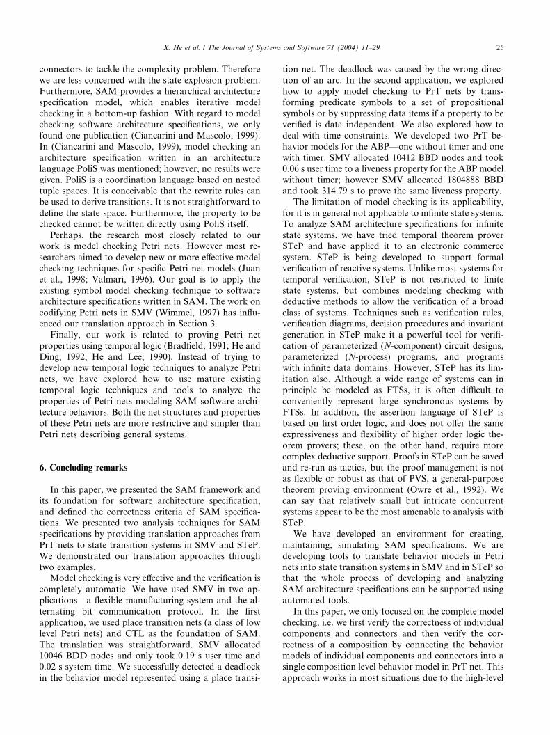
In this paper, we only focused on the complete model

checking, i.e. we first verify the correctness of individual

components and connectors and then verify the cor-

rectness of a composition by connecting the behavior

models of individual components and connectors into asingle composition level behavior model in PrT net. This

approach works in most situations due to the high-level


abstraction of a software architecture specification.

However the connected composition level behavior

model can be quite large in some situations to prevent

the effective use of symbolic model checking technique

or theorem proving. To solve this problem, we are

investigating several compositional model checkingtechniques. Among the various proposed automated

compositional verification techniques in temporal logic

(Berezin et al., 1998; Clarke et al., 1994; Grumberg and

Long, 1994) and in Petri nets (Juan et al., 1998; Valmari,

1996), we found that the interface module technique

(Berezin et al., 1998) and the IO graph technique (Juan

et al., 1998) are most relevant to our research. We are

currently focusing on how to adapt these compositionalverification techniques to analyze SAM software archi-

tectural specifications. We are also studying composi-

tional temporal logic proving techniques developed in

(Abadi and Lamport, 1991, 1993).

Acknowledgements

We thank two anonymous reviewers for their helpful

comments, which help improve the presentation of this

paper. This work is supported in part by NSF under

grant HDR-9707076 and CCR-0098120, and by NASA

under grant NAG 2-1440.

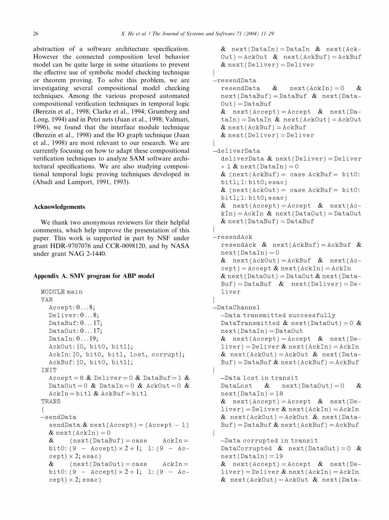
Appendix A. SMV program for ABP model

MODULE main

VAR

Accept:0 . . . 8;Deliver:0 . . . 8;DataBuf:0 . . . 17;DataOut:0 . . . 17;DataIn:0 . . . 19;AckOut:{0, bit0, bit1};

AckIn:{0, bit0, bit1, lost, corrupt};

AckBuf:{0, bit0, bit1};

INIT

Accept¼8 & Deliver¼0 & DataBuf¼1 &

DataOut¼0 & DataIn¼0 & AckOut¼0 &

AckIn¼bit1 & AckBuf¼bit1TRANS

(

–sendData

sendData & next(Accept)¼(Accept � 1)

& next(AckIn)¼0& (next(DataBuf)¼case AckIn¼bit0:(9 � AcceptÞ � 2þ 1; 1:(9 � Ac-

ceptÞ � 2;esac)& (next(DataOut)¼case AckIn¼bit0:(9 � AcceptÞ � 2þ 1; 1:(9 � Ac-

ceptÞ � 2;esac)

& next(DataIn)¼DataIn & next(Ack-

Out)¼AckOut & next(AckBuf)¼AckBuf& next(Deliver)¼Deliver

j–resendData

resendData & next(AckIn)¼0 &next(DataBuf)¼DataBuf & next(Data-

Out)¼DataBuf& next(Accept)¼Accept & next(Da-

taIn)¼DataIn & next(AckOut)¼AckOut& next(AckBuf)¼AckBuf& next(Deliver)¼Deliver

j–deliverData

deliverData & next(Deliver)¼Deliver+ 1 & next(DataIn)¼0& (next(AckBuf)¼ case AckBuf¼ bit0:

bit1;1:bit0;esac)

& (next(AckOut)¼ case AckBuf¼ bit0:

bit1;1:bit0;esac)

& next(Accept)¼Accept & next(Ac-

kIn)¼AckIn & next(DataOut)¼DataOut& next(DataBuf)¼DataBuf

j–resendAck

resendAck & next(AckBuf)¼AckBuf &

next(DataIn)¼0& next(AckOut)¼AckBuf & next(Ac-

cept)¼Accept & next(AckIn)¼AckIn& next(DataOut)¼DataOut & next(Data-

Buf)¼DataBuf & next(Deliver)¼De-liver

j–DataChannel

–Data transmitted successfully

DataTransmitted & next(DataOut)¼0 &

next(DataIn)¼DataOut& next(Accept)¼Accept & next(De-

liver)¼Deliver & next(AckIn)¼AckIn& next(AckOut)¼AckOut & next(Data-

Buf)¼DataBuf & next(AckBuf)¼AckBufj–Data lost in transit

DataLost & next(DataOut)¼0 &

next(DataIn)¼18& next(Accept)¼Accept & next(De-


Buf)¼DataBuf & next(AckBuf)¼AckBufj–Data corrupted in transit

DataCorrupted & next(DataOut)¼0 &

next(DataIn)¼19& next(Accept)¼Accept & next(De-



Buf)¼DataBuf & next(AckBuf)¼AckBufj–Ack Channel

–Ack transmitted successfully

AckTransmitted & next(AckOut)¼0 &

next(AckIn)¼AckOut& next(Accept)¼Accept & next(De-

liver)¼Deliver & next(DataOut)¼DataOut

& next(DataBuf)¼DataBuf & next(Ack-

Buf)¼AckBuf & next(DataIn)¼DataInj–Ack lost in transit

AckLost & next(AckOut)¼0 & next(Ac-

kIn)¼lost& next(Accept)¼Accept & next(De-



Buf)¼AckBuf & next(DataIn)¼DataInj–Ack corrupted in transit

AckCorrupted & next(AckOut)¼0 &

next(AckIn)¼corrupt& next(Accept)¼Accept & next(De-



Buf)¼AckBuf & next(DataIn)¼DataInj–selfloop for deadlock

deadlock & next(Accept)¼Accept &

next(Deliver)¼Deliver& next(DataOut)¼DataOut & next(Ac-

kIn)¼AckIn & next(AckOut)¼AckOut& next(DataBuf)¼DataBuf & next(Ack-

Buf)¼AckBuf & next(DataIn)¼DataIn)DEFINE

sendData:¼Accept>0 & ((DataBuf mod

2)¼0 & AckIn¼bit0 | (DataBuf mod

2)¼1 & AckIn¼bit1);resendData:¼DataBuf>0 & (Ac-

kIn¼lost | AckIn¼corrupt |

(DataBuf mod 2)¼1 & AckIn¼bit0 |

(DataBuf mod 2)¼0 & AckIn¼bit1);deliverData:¼DataIn>0 & DataIn<¼17

& ((DataIn mod 2)¼0 & AckBuf¼bit1 |(DataIn mod 2)¼1 & AckBuf¼bit0);

resendAck:¼AckBuf!¼0 & DataIn>0 &

(DataIn¼18|DataIn¼19 |

(DataIn mod 2)¼1 & AckBuf¼bit1 |

(DataIn mod 2)¼0 & AckBuf¼bit0);DataTransmitted:¼DataOut>0;DataLost:¼DataOut>0;DataCorrupted:¼DataOut>0;

AckTransmitted:¼AckOut!¼0;AckLost:¼AckOut!¼0;AckCorrupted:¼AckOut!¼0;deadlock:¼!(sendData|resend-Data|deliverData|resendAck|Data-

Transmitted|AckTransmitted);

FAIRNESS

(DataIn>0 & DataIn<18) & (AckIn¼bit0| AckIn¼bit1)

SPEC

(AF Deliver¼8)SPEC

(AG((deliverData & !next(deliver-

Data))->(DataIn/2¼Deliver+1)))

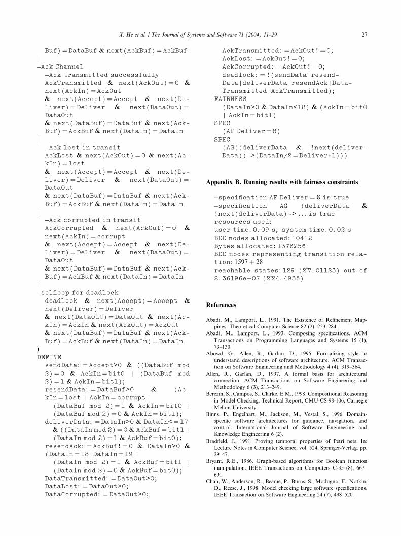
Appendix B. Running results with fairness constraints

–specification AF Deliver ¼ 8 is true

–specification AG (deliverData &!next(deliverData) -> . . . is true

resources used:

user time:0.09 s, system time:0.02 s

BDD nodes allocated:10412

Bytes allocated:1376256

BDD nodes representing transition rela-

tion:1597þ 28

reachable states:129 (2̂ 7.01123) out of

2.36196eþ07 (2̂ 24.4935)

References

Abadi, M., Lamport, L., 1991. The Existence of Refinement Map-

pings. Theoretical Computer Science 82 (2), 253–284.

Abadi, M., Lamport, L., 1993. Composing specifications. ACM

Transactions on Programming Languages and Systems 15 (1),

73–130.

Abowd, G., Allen, R., Garlan, D., 1995. Formalizing style to

understand descriptions of software architecture. ACM Transac-

tion on Software Engineering and Methodology 4 (4), 319–364.

Allen, R., Garlan, D., 1997. A formal basis for architectural

connection. ACM Transactions on Software Engineering and

Methodology 6 (3), 213–249.

Berezin, S., Campos, S., Clarke, E.M., 1998. Compositional Reasoning

in Model Checking. Technical Report, CMU-CS-98-106, Carnegie

Mellon University.

Binns, P., Engelhart, M., Jackson, M., Vestal, S., 1996. Domain-

specific software architectures for guidance, navigation, and

control. International Journal of Software Engineering and

Knowledge Engineering 6 (2).

Bradfield, J., 1991. Proving temporal properties of Petri nets. In:

Lecture Notes in Computer Science, vol. 524. Springer-Verlag. pp.

29–47.

Bryant, R.E., 1986. Graph-based algorithms for Boolean function

manipulation. IEEE Transactions on Computers C-35 (8), 667–

691.

Chan, W., Anderson, R., Beame, P., Burns, S., Modugno, F., Notkin,

D., Reese, J., 1998. Model checking large software specifications.

IEEE Transaction on Software Engineering 24 (7), 498–520.


Ciancarini, P., Mascolo, C., 1999. Model checking a software

architecture. In: Proceedings of ROSATEA: International Work-

shop on the Role of Software Architecture in Analysis and Testing,

Software Engineering Notes. vol. 24, p. 4.

Clarke, E., Wing, J., 1996. Formal methods: state of the art and future.

ACM Computing Surveys 28 (4), 626–643.

Clarke, E.M., Emerson, E.A., Sistla, A.P., 1986. Automatic verifica-

tion of finite-state concurrent systems using temporal logic spec-

ifications. ACM Transaction on Programming Languages and

Systems 8 (2), 244–263.

Clarke, E.M., Grumberg, O., Long, D.E., 1994. Model Checking and

Abstraction. ACM Transaction on Programming Language and

Systems 16 (5), 1512–1542.

Clarke, E.M., Grumberg, O., Peleg, D., 1999. Model Checking. The

MIT Press.

Genrich, H., Lautenbach, K., 1981. System modeling with high-level

Petri nets. Theoretical Computer Science 13, 109–136.

Grumberg, O., Long, D., 1994. Model checking and modular

verification. ACM Transaction on Programming Language and

Systems 16 (3), 843–871.

He, X., 1996. A formal definition of hierarchical predicate transition

nets. In: Proceedings of the 17th International Conference on

Application and Theory of Petri Nets (ICATPN’96). Lecture Notes

in Computer Science, 1091, Osaka, Japan, pp. 212–229.

He, X., Deng, Y., 2000. Specifying software architectural connectors in

SAM. International Journal of Software Engineering and Knowl-

edge Engineering 10 (4), 411–432.

He, X., Deng, Y., 2002. A framework for developing and analyzing

software architecture specifications in SAM. The Computer Jour-

nal 45 (1), 111–128.

He, X., Ding, Y., 1992. A temporal logic approach for analyzing safety

properties of predicate transition nets. In: Proceedings of the 12th

IFIP World Computer Congress (Information Processing’92).

Madrid, Spain, pp. 127–133.

He, X., Lee, J.A.N., 1990. Integrating predicate transition nets and

first order temporal logic in the specification of concurrent systems.

Formal Aspects of Computing 2 (3), 226–246.

Hoare, C.A.R., 1985. Communicating Sequential Processes. Prentice-

Hall International.

Inverardi, P., Richardson, D., 1999. ROSATEA: International Work-

shop on the Role of Software Architecture in Analysis and Testing.

In: Software Engineering Notes, vol. 24. p. 4.

Inverardi, P., Wolf, A., 1995. Formal specification and analysis of

software architectures using the chemical abstract machine model.

IEEE Transactions on Software Engineering 21 (4), 373–386.

Juan, E., Tsai, J.P., Murata, T., 1998. Compositional verification of

concurrent systems using Petri-net-based condensation rules. ACM

Transactions on Programming Languages and Systems 20 (5), 917–

979.

Lamport, L., 1994. The temporal logic of actions. ACM Transactions

on Programming Languages and Systems 16 (3), 872–923.

Luckham, D.C., Kenney, J., Augustin, L., et al., 1995. Specification

and analysis of system architecture using rapide. IEEE Transac-

tions on Software Engineering 21 (4), 336–355.

Maidl, M., 2000. The Common Fragment of CTL and LTL. In:

Proceeding of 41st Symposium on Foundations of Computer

Science. pp. 643–652.

Mandrioli, D., Morzenti, A., Pezze, M., Pietro, P., Silva, S., 1996. A

Petri net and logic approach to the specification and verification of

real time systems. In: Heitmeyer, C., Mandrioli, D. (Eds.), Formal

Methods for Real time Computing. John Wiley & Sons Ltd.

Manna, Z., Anuchitanukul, A., Bjorner, N., Browne, A., Chang, E.,

Colon, M., de Alfaro, L., Devarajan, H., Sipma, H., Uribe, T.,

1994. STeP: The Stanford Temporal Prover, Technical Report

STAN-CS-TR-94-1518, Computer Science Department, Stanford

University.

Manna, Z., Pnueli, A., 1992. The Temporal Logic of Reactive and

Concurrent Systems. Springer-Verlag.

McMillan, K.L., 1993. Symbolic Model Checking. Kluwer Academic

Publishers, Boston.

Medvidovic, N., Taylor, R., 2000. A classification and comparison

framework for software architecture description languages. IEEE

TSE 26 (1), 70–93.

Murata, T., 1989. Petri nets: properties, analysis and applications.

Proceedings of the IEEE 77 (4), 541–580.

Owre, S., Rushby, J.M., Shankar, N., 1992. PVS: a prototype

verification system. In: Kapur, D. (Ed.), 11th International

Conference on Automated Deduction (CADE). In: Lecture

Note in Artificial Intelligence, vol. 607. Springer-Verlag, pp. 748–

752.

Richardson, D., Wolf, A., 1996. Software testing at the architectural

level. In: Proceedings of the 2nd International Software Architec-

ture Workshop. pp. 68–71.

Shaw, M., 2001. The coming-of-age of software architecture research.

In: Proceedings of International Conference on Software Engi-

neering. Toronto, pp. 656–664.

Shaw, M., Deline, R., Klein, D., et al., 1995. Abstractions for software

architecture and tools to support them. IEEE Transactions on

Software Engineering 21 (4), 314–335.

Spivey, J., 1992. Z Reference Manual, second ed. Cambridge Univer-

sity Press.

Sreemani, T., Atlee, J., 1996. Feasibility of model checking software

requirements: a case study. In: Proceedings of the 11th Annual

Conference On Computer Assurance. Gaithersburg, MD, pp. 77–

88.

Valmari, A., 1996. Compositionality in state space verification

methods. Lecture Notes in Computer Science 1091, 29–56.

Wang, J., He, X., Deng, Y., 1999. Introducing software architecture

specification and analysis in SAM through an example. Informa-

tion and Software Technology 41 (7), 451–467.

Wimmel, G., 1997. A BDD-based Model Checker for the PEP Tool.

Technical Report, Department of Computer Science, University of

Newcastle.

Xudong He received the BS and MS degrees in computer science fromNanjing University, China, in 1982 and 1984, respectively. He receivedthe Ph.D. degree in computer science from Virginia Polytechnic In-stitute & State University (Virginia Tech) in 1989.

He joined the faculty in the School of Computer Science at FloridaInternational University (FIU) in 2000, and is an associate professor ofthe School of Computer Science and the Director of the Center forAdvanced Distributed System Engineering. Prior to joining FIU, hewas an associate professor in the Department of Computer Science atNorth Dakota State University since 1989. His research interests in-clude formal methods, especially Petri nets, and software testingtechniques. He has published over 50 papers in the above areas.

Dr. He is a member of the Association for Computing Machinery,and the IEEE Computer Society.

Huiqun Yu received his B.S. degree from Nanjing University in 1989,M.S. degree from East China University of Science and Technology(ECUST) in 1992, and Ph.D. degree from Shanghai Jiaotong Uni-versity in 1995, all in computer science. Currently, he is a visitingscholar in the School of Computer Science at Florida InternationalUniversity. He holds a Professor position in the Department ofComputer Science and Engineering at ECUST. His research interestsinclude formal methods for complex software systems, hardware/software co-design of embedded systems, and techniques for analysisof software architecture.

Tianjun Shi received his B.S. in Manufacturing Engineering fromBeijing University of Aeronautics and Astronautics in 1995 and M.S.in Computer Science from Beijing Institute of Information and Con-trol in 1998. He is currently a Ph.D. candidate in Computer Science atFlorida International University. His research interests include soft-ware architecture, formal methods, distributed computing and net-working.


Junhua Ding received a B.S. degree in Computer Engineering fromChina University of Geosciences in 1994, and an M.S degree inComputer Science from Nanjing University in 1997. He is presently aPh.D. candidate in the School of Computer Science at Florida Inter-national University. He is also a software engineer in the CytomicsDevelopment Center of Beckman Coulter Inc. His research interestsinclude modeling and analysis of distributed systems, Cytomics systemdevelopment.

Yi Deng is the Director of the School of Computer Science at theFlorida International University (FIU) – The State University ofFlorida at Miami. From August 2000 to May 2002, he was with theUniversity of Texas at Dallas (UT-Dallas) as the Managing Directorof the Embedded Software Center and Associate Professor of Com-puter Science in the School of Engineering and Computer Science.Prior to joining UT-Dallas, he had been an Associate Professor of

Computer Science at FIU and the founding Director of Center forAdvanced Distributed Systems Engineering (CADSE) – a universityresearch center designated by the Florida Board of Regents. His re-search interests include component-based software engineering, soft-ware architecture, formal methods for complex systems, modeling andanalysis of software security systems and middleware. He has pub-lished over 60 papers in various journals and conferences. He hasbeen the Principal Investigator (PI) or Co-PI of fourteen (14) researchawards of over $7 million from the National Science Foundation(NSF), US Air Force Office of Scientific Research (AFOSR), USArmy Research Office (ARO), US Air Force Rome Laboratory andthe National Aeronautics and Space Administration (NASA), as wellas from industry. Dr. Deng is an editor for the International Journalof Software Engineering and Knowledge Engineering and has beenprogram committee chair or member for several conferences. He re-ceived his Ph.D. in Computer Science from University of Pittsburghin 1992 and is a member of ACM, EEE and IEEE Computer Society.

Documents

Formally analyzing software architectural specifications using SAM