Computers and Structures 132 (2014) 65–74

Contents lists available at ScienceDirect

Computers and Structures

journal homepage: www.elsevier .com/locate /compstruc

Form-finding of compressive structures using Prescriptive DynamicRelaxation

0045-7949/$ - see front matter � 2013 Elsevier Ltd. All rights reserved.http://dx.doi.org/10.1016/j.compstruc.2013.10.018

⇑ Corresponding author. Tel.: +1 4102416510.E-mail address: abhalper@princeton.edu (A.B. Halpern).

Serguei Bagrianski, Allison B. Halpern ⇑Department of Civil and Environmental Engineering, Princeton University, Engineering Quadrangle E325, Princeton, NJ 08544, USA

a r t i c l e i n f o

Article history:Received 20 February 2013Accepted 31 October 2013Available online 5 December 2013

Keywords:Dynamic RelaxationForm-findingConcrete shellsFootbridgesSegmentationCompressive structures

a b s t r a c t

This paper presents an adaptation of the Dynamic Relaxation method for the form-finding of small-straincompressive structures that can be used to achieve project-specific requirements such as prescribed ele-ment lengths. Novel truss and triangle elements are developed to permit large strains in the form-findingmodel while anticipating the small-strain behavior of the realized structure. Forcing functions are formu-lated to permit element length prescription using a new iterative technique termed Prescriptive DynamicRelaxation (PDR). Case studies of a segmental concrete shell and a pedestrian steel bridge illustrate thepotential for using PDR to achieve economic and environmentally considerate structural solutions.

� 2013 Elsevier Ltd. All rights reserved.

1. Dynamic Relaxation and structural form-finding

Dynamic Relaxation (DR) was first proposed by Day in 1965 asan alternative analysis tool for indeterminate structures [1]. Usingequations derived from the second law of motion, DR transforms anonlinear static problem into a pseudo-dynamic one in which thedisplacements are updated via a time-stepping procedure toachieve a sufficiently equilibrated state. Since its inception, DRhas been used as a nonlinear solver for a broad range of analyticalproblems [2] but was first used as a form-finding tool for tensilestructures by Barnes [3–6]. DR has since been employed for theform-finding of cable-membrane structures [7], grid shells [8,9],continuous shells [10,11], and tensegrity structures [12,13].

Form-finding techniques can be assigned to three categories:physical hanging models, equilibrium methods, and optimizationschemes. Physical hanging models, like those used by Antoni Gaudi[14], Heinz Isler [15], and Frei Otto [16], typically rely on inexten-sible cable networks to create purely axial systems under a gravi-tational load. Equilibrium methods such as Dynamic Relaxation,force density [17], stress distribution [18], thrust-network analysis[19], and particle-spring [20] use iteration algorithms to manipu-late nodal geometry to equilibrate method-specific internal forceswith applied external loads. Optimization schemes manipulatecontrol parameters, such as nodal coordinates, of a structural sys-tem to provide an optimal solution for one criterion [21] or providea Pareto Front for multiple criteria [22].

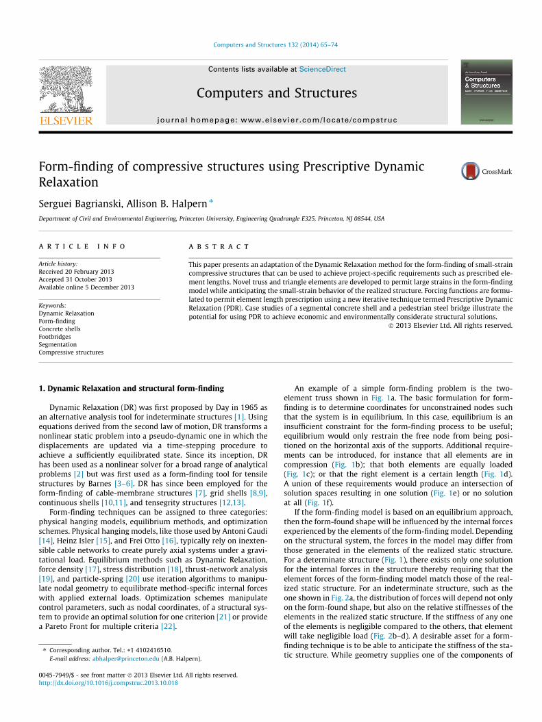
An example of a simple form-finding problem is the two-element truss shown in Fig. 1a. The basic formulation for form-finding is to determine coordinates for unconstrained nodes suchthat the system is in equilibrium. In this case, equilibrium is aninsufficient constraint for the form-finding process to be useful;equilibrium would only restrain the free node from being posi-tioned on the horizontal axis of the supports. Additional require-ments can be introduced, for instance that all elements are incompression (Fig. 1b); that both elements are equally loaded(Fig. 1c); or that the right element is a certain length (Fig. 1d).A union of these requirements would produce an intersection ofsolution spaces resulting in one solution (Fig. 1e) or no solutionat all (Fig. 1f).

If the form-finding model is based on an equilibrium approach,then the form-found shape will be influenced by the internal forcesexperienced by the elements of the form-finding model. Dependingon the structural system, the forces in the model may differ fromthose generated in the elements of the realized static structure.For a determinate structure (Fig. 1), there exists only one solutionfor the internal forces in the structure thereby requiring that theelement forces of the form-finding model match those of the real-ized static structure. For an indeterminate structure, such as theone shown in Fig. 2a, the distribution of forces will depend not onlyon the form-found shape, but also on the relative stiffnesses of theelements in the realized static structure. If the stiffness of any oneof the elements is negligible compared to the others, that elementwill take negligible load (Fig. 2b–d). A desirable asset for a form-finding technique is to be able to anticipate the stiffness of the sta-tic structure. While geometry supplies one of the components of

Fig. 1. Form-finding of a determinate structure. Shaded areas indicate the search space imposed by the constraints.

Fig. 2. Form-finding of an indeterminate structure.

66 S. Bagrianski, A.B. Halpern / Computers and Structures 132 (2014) 65–74

static stiffness, material properties and element dimensions alsocontribute.

Neither equilibrium methods nor physical models have typi-cally afforded significant opportunity for introducing materialproperties; in fact, a recent review of form-finding techniquesidentified the form-finding process as ‘material independent’[23]. It is also common to consider the form-found shape as astarting point to which dimensions can be assigned [24], e.g., bydensity distribution [25,26]. While optimization schemes rely oncomputational models with accurately defined material proper-ties, they are not well suited for finding funicular shapes. Forcompressive systems, the most efficient form is one that relieson a resolution of external loads through axial internal forces[27]. The physical hanging models exemplify Hooke’s frequentlyused adage, ‘as hangs the flexible cable so, inverted, stand thetouching pieces of an arch,’ [28] by relying on cables that cannotresist bending to produce shapes that when inverted are entirelyin compression.

It is possible to identify three desirable qualities for a form-finding process for compressive systems:

1. Elements can only transmit axial loads2. Material properties and dimensions of the realized structure are

included as parameters in the form-finding process3. Project-specific requirements can be introduced systematically

Because DR is rooted in the analysis of real structures, it is wellsuited for the form-finding of cable-membrane structures as itsimulates realistic structural behavior [7]. Accordingly, the authorspropose that DR is the best suited of the equilibrium methods forincorporating realistic material properties to produce an axially-driven form-finding process for compressive structures. The basicDR algorithm used for this study is presented in Section 2. InSection 3, we introduce a truss element and a triangular membraneelement for the form-finding of compressive structures. InSection 4, we introduce the concept of Prescriptive DynamicRelaxation (PDR), which permits the achievement of certainsystem requirements through a modification of the DR process.In Section 5, we offer a method to achieve prescribed elementlengths using forcing functions in PDR. In Section 6, we providecase studies demonstrating application to a concrete shell and asteel pedestrian bridge.

2. The Dynamic Relaxation algorithm

The DR method presented in this section is adapted from Barnes[5]. First, the Residual, Rt

i;x, at time t is calculated:

Rti;x ¼ Pi;x þ

Xj

XcoðkÞ¼i

Fti;j;k;x ð1Þ

where the indices i, j, k, and x refer to global node number, elementnumber, local node number, and directional degree of freedom; theco() operator converts local numbering to global numbering; Pi,x isthe applied external load; and Ft

i;j;k;x is the element force vector.Next, the updated velocity, VtþDt=2

i;x , is found:

VtþDt=2i;x ¼

VtþDt=2i;x þ Dt

MiRt

i;x if ci;x ¼ 0

0 if ci;x ¼ 1

( )ð2Þ

where Dt is the time step, Mi is the fictitious nodal mass, and ci,x isthe binary restraint value for the degree of freedom (0 if free, 1 ifrestrained). The new nodal coordinates, xtþDt

i , are then found:

xtþDti ¼ xt

i þ DtVtþDt=2i;x ð3Þ

To reach equilibrium, it is necessary to damp the system. Day intro-duced viscous damping by multiplying the velocity term, Vt�Dt=2

i;x , byan arbitrary damping constant, 0 < KV < 1 [1]. Kinetic damping, analternative to viscous damping, was first introduced by Cundall in1976 [29]. To achieve kinetic damping, the kinetic energy, Kt, istracked at each iteration:

Kt ¼X

i

MijVt�Dt=2i j2 ð4Þ

When the kinetic energy is at a maximum (corresponding to mini-mum strain energy), the velocity is set to zero. The iterations areterminated when the system achieves a prescribed level of equilib-rium. In this paper, a stringent criterion, fconv� 1, is implemented:

max8i

ffiffiffiffiffiffiffiffiffiffiffiffiffiffiffiffiffiffiffiffiffiffiffiffiffiffiffiffiffiffiffiffiffiffiffiffiffiffiffiffiPx Rt

i;x

� �2ð1� ci;xÞP

xðPi;xÞ2 þ ðWoi Þ

2

vuuut � fconv ð5Þ

The numerator is the maximum of the current residuals, Rti;x, and the

denominator is the maximum of the applied loads calculated as asum of the external loads, Pi,x, and initial self-weight element con-tributions to each node, Wo

i .The DR iterative process can be summarized in three basic

steps:

1. Initialize model (e.g., starting geometry, material proper-ties, boundary conditions, and loading)

2. Calculate element forces and residuals. If fconv is achieved,output results and terminate.

3. Calculate velocities (adjusted to chosen method of damp-ing) and nodal coordinates. Go to step 2.

S. Bagrianski, A.B. Halpern / Computers and Structures 132 (2014) 65–74 67

One ambiguity in this process is how the internal element forcesare calculated in Eq. (1). Ideally the forces generated in the form-finding model will correlate closely to those in the realized struc-ture. To achieve this effect it is necessary to incorporate materialproperties and element dimensions into the formulation for calcu-lating element forces.

3. Small strain analogy for axial elements

To achieve a compressive form-finding model that closely antic-ipates the realized static system, axial elements are derived usingthree basic concepts. The first concept is to make strain relativeto the static system. Because the geometry of the static system isnot known beforehand, the geometry at the current time step isused; once the form-finding system reaches sufficient equilibrium,the current geometry will match the static geometry thereby vali-dating the strain state. The second concept is to imitate smallstrain behavior in a model undergoing large deformations. Becausethe form-finding problem is not to accurately model large strainbehavior, but to predict the linear-elastic behavior of a static sys-tem, rigorously adhering to large strain mechanics is not pertinent.The third concept is to make the form-finding system significantlymore flexible than the form-found shape while still maintainingthe desirable relative element stiffness. This modified stiffnesshas been documented [11] but has not seen systematic implemen-tation. The system Elasticity Factor, uE, is thus defined as:

uE ¼EM

E� 1 ð6Þ

where E is the elastic modulus of the realized static system and EM

is the reduced elastic modulus used for form-finding. Throughoutthis section, the subscripts for element number are removed forclarity of presentation. Both truss and triangle elements are dis-cussed in their local coordinate system; for implementation theywould be rotated to global coordinates.

3.1. Truss element

The axial force in a truss element using static analysis can bestated as:

F ¼ EA0e ð7Þ

where E, A0, and e are the elastic modulus, cross-sectional area, andstrain, respectively. For the form-finding formulation, the staticlength is not known beforehand. As such, strain is calculated withreference to the length at the current time, t:

et ¼ Lr � Lt

Lt ð8Þ

The relaxed length, Lr, in this formulation is a parameter set withinthe form-finding process. Large elongations in the form-finding pro-cess will inevitable produce large strains. Typically, large deforma-tions require the use of the Green–Lagrange strain tensor:

e ¼ 12ðU2 � IÞ ð9Þ

where U is the right stretch tensor and I is the identity tensor [30].The objective of the form-finding process is not, however, to accu-rately model large strain effects but to predict small strain effects.Given the proposed choice of strain reference, the quadratic termsonly serve to maintain compatibility of the relaxed geometries. Be-cause the relaxed element lengths are treated as parameters, thecompatibility of the relaxed form-found geometry is not necessaryand so second order effects are omitted. Once the Elasticity Factor,uE, is introduced, the force vector, Ft, for a form-finding truss ele-ment in local coordinates becomes:

Ft ¼ uEEA0Lr � Lt

Lt f�1 1g ð10Þ

This formulation will achieve accurate relative stiffness among ele-ments but will still permit control of the shape without arbitrarilymodifying the material properties or element dimensions.

3.2. Triangular membrane element formulation

There is a wide array of techniques for the form-finding of con-tinuous shells. The governing approach is to approximate the con-tinuous surface using link element meshes. In the context of thispaper, the link element is defined as one whose internal forcesare influenced by the relative position of its two end points; two-noded elements assigned forces that are mechanically equivalentto those generated in a three-noded membrane element [5,7] areconsidered membrane elements. While refinement of the meshcan always produce better assumptions of continuity, the link ele-ment cannot capture membrane effects. The anisotropic nature ofthis method was a criticism raised by Eduardo Torroja of Isler’shanging cloth models [24] and can be extended to any of the mod-ern techniques that form-find continuous shells using link ele-ments [19,20]. While these link-element methods all producesensible shapes, they are not designed to anticipate membranecapacity.

In finite element analysis, the simplest membrane element isthe three-node constant stress triangular element [31]. Becausethe displacement field is linear, yielding constant strains and stres-ses, the constant stress triangle can be treated as a two-dimen-sional analogy to the one-dimensional truss. The generalformulation for the force vector, F, for the small-strain triangularmembrane element in local coordinates can be represented as:

F ¼ hABT DBu ð11Þ

where h, A, B, D, and u correspond to the thickness, triangle area,strain–displacement matrix, plane stress material moduli matrix,and nodal displacements, respectively. This equation can be brokendown into the respective equilibrium, constitutive, and kinematiccomponents:

F ¼ hABTr ð12-aÞ

r ¼ De ð12-bÞ

e ¼ Bu ð12-cÞ

Available membrane form-finding techniques typically assume asensible stress state and rely only on the equilibrium relationshipto generate a force vector. For the form-finding of fabrics, the stressstate can be represented by the prescribed warp and weft prestress[5,7]. For the form-finding of compressive shells, isotropic stress tri-angles have been used but require link elements along the systemboundary to simulate a free edge [18]. To best predict the mem-brane stiffness of the static triangle, the form-finding element is de-rived using all three equilibrium, constitutive, and kinematiccomponents.

The kinematic relationship for large strain is defined by thetwo-dimensional expression of the Green–Lagrange tensor:

et ¼exx

eyy

exy

8><>:

9>=>; ¼

ux þ 12 ðu2

x þ v2x Þ

vy þ 12 ðu2

y þ v2yÞ

vx þ uy þ uxuy þ vxvy

8><>:

9>=>; ð13Þ

While it can be argued that the quadratic terms should be dis-carded, strain proves rotationally inconsistent and second order ef-fects must therefore be included. Given the proposed mapping of

Fig. 3. Relaxed (r) and deformed (t) geometries mapped to xy plane.

68 S. Bagrianski, A.B. Halpern / Computers and Structures 132 (2014) 65–74

relaxed and deformed geometry (Fig. 3), the deformations can beexpressed explicitly as:

ux uy vx vyf g ¼ xr2 � xt

2

xr2

xr3xt

2 � xr2xt

3

xt2yt

30

yr3 � yt

2

yt3

� �ð14Þ

where the coordinates are found to be:

x1 y1 x2 y2 x3 y3f g ¼ 0 0 L1 0 L3 cos b L3 sin bf gð15Þ

As with the truss element, strain is referenced to the deformed con-figuration, permitting accurate prediction of the forces in the staticstructure.

The constitutive relation for plane stress, adjusted for reducedstiffness, provides the stress tensor:

r ¼ uEDet ð16Þ

where D is the plane stress material moduli matrix:

D ¼ E1� m2

1 m 0m 1 00 0 1� m

264

375 ð17Þ

where m is Poisson’s ratio. Using the equilibrium relationship, thestress is then numerically integrated over the deformed area ofthe triangle using Eq. (12-a) where the strain–displacement matrixcan be expressed as:

Bt ¼ 1At

yt2 � yt

1 0 yt3 � yt

2 0 yt1 � yt

3 00 xt

1 � xt2 0 xt

2 � xt3 0 xt

3 � xt1

xt1 � xt

2 yt2 � yt

1 xt2 � xt

3 yt3 � yt

2 xt3 � xt

1 yt1 � yt

3

264

375ð18Þ

where the current area can be calculated as:

At ¼ 12

xt2yt

3 ð19Þ

The complete formulation can thus be expressed as:

Ft ¼ uEtAtðBtÞT Det ð20Þ

To provide an example of the effectiveness of the triangle element, asimply supported, 14.1 m � 14.1 m square plan is form-found withthree different schemes – a rectangular truss mesh, a triangulartruss mesh, and a triangular membrane mesh. The shapes areform-found under identical point loads of 2 kN placed at every nodeand the elasticity modifier is tailored for each system to achieve aheight of 2.0 m. The form-found geometries are then analyzed inLUSAS [32] using a 1:1 mesh, representing every triangular element

as a TSM3 plane stress membrane element. Fig. 4 shows thedisplacement field and principal compressive stresses normalizedto the maximum value among all shapes.

The maximum stresses are �0.221, �0.225, and �0.204 MPa;the maximum deflections are 0.106, 0.136, and 0.098 mm for thethree shapes, respectively. The triangle membrane formulationnot only produces the lowest stresses and deflections, but alsoyields the most comprehensible overall system behavior. Theedges of the two truss schemes demonstrate large deformationcoupled with high stresses, which could suggest unfavorable sec-ond order effects such as buckling. By contrast, the triangularmembrane form-found shape deforms with a gradual increase to-wards the center of the span corresponding with the regions oflowest stress. The benefits of the triangle membrane solution existbecause of the ability of the triangle membrane form-findingscheme to predict the stresses of the analytical model; the princi-pal stresses in the form-finding model only differ from those in theanalytical model by an average of 2.1%.

4. Framework for Prescriptive Dynamic Relaxation

Having established the iterative scheme and element formula-tions for the basic DR method for compressive structures, it is pos-sible to outline the full set of variables in the system (see Table 1).

The outputs include coordinates, lengths, forces and stresseswhen t = f, which is defined as the time when equilibrium conver-gence has been achieved. The transient variables facilitate conver-gence, but do not influence the solution beyond the accuracy andspeed of convergence. Both structural and algorithmic parametersmodify the outcome, but any modification to the structural param-eters is directly reproduced in the static structure. The algorithmicparameters of initial element lengths and elasticity modifiers canbe considered arbitrary and thus provide the most flexible param-eters for attaining certain requirements. PDR exploits the algorith-mic parameters to systematically achieve prescribed requirementsby adding a feedback loop (Step 4) to the basic DR process (Steps1–3) presented below:

1. Initialize model (e.g., starting geometry, material properties,boundary conditions, and loading)

2. Calculate element forces and residuals. If fconv is achieved, go tostep 4.

3. Calculate velocities (adjusted to chosen method of damping)and nodal coordinates. Go to step 2.

4. If system prescriptions are met, output results and terminateprogram. If prescriptions have not been met, use forcing func-tions to reassign model parameters and go to step 2.

5. Length prescription forcing functions

In this paper, relaxed lengths are used to generate prescribedelement geometries. The control of element geometry is particu-larly desirable for economic reasons. If the manufacturing meansof producing the segments are known, the form-found shape canbe tailored to meet the manufacturing constraints of an economi-cally beneficial process. Segmental schemes, particularly those thatrely on constant length elements, have seen economic success inpast systems such as the Pegram Truss [33], American Standardkit bridges [34], lamella roofs [35], precast coffers [36], and precastsegmental shells [37]. Documented uses of form-finding with localgeometry control are limited to distortion control [38,39], nodalplanarity [8], tensegrity [40], and prestress control [41].

To achieve prescribed element lengths, the strain at equilibriumconvergence can be used to back-calculate to a relaxed geometrythat under the same strain would produce the prescribed geome-

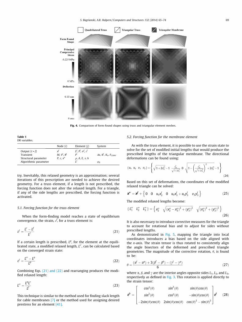
Fig. 4. Comparison of form-found shapes using truss and triangular element meshes.

Table 1DR variables.

Node (i) Element (j) System

Output (t = f) xf Lf, Ff, rf, ef

Transient M, Vt, Rt Ft Dt, Kt, KV, FCONV

Structural parameter P, c, xo q, A, E, v, hAlgorithmic parameter Lr uE

S. Bagrianski, A.B. Halpern / Computers and Structures 132 (2014) 65–74 69

try. Inevitably, this relaxed geometry is an approximation; severaliterations of this prescription are needed to achieve the desiredgeometry. For a truss element, if a length is not prescribed, theforcing function does not alter the relaxed length. For a triangle,if any of the side lengths are prescribed, the forcing function isactivated.

5.1. Forcing function for the truss element

When the form-finding model reaches a state of equilibriumconvergence, the strain, ef, for a truss element is:

ef ¼ Lr � Lf

Lfð21Þ

If a certain length is prescribed, Lp, for the element at the equili-brated state, a modified relaxed length, Lr0, can be calculated basedon the converged strain state:

ef ¼ Lr0 � Lp

Lp ð22Þ

Combining Eqs. (21) and (22) and rearranging produces the modi-fied relaxed length:

Lr0 ¼ LpLr

Lfð23Þ

This technique is similar to the method used for finding slack lengthfor cable membranes [7] or the method used for assigning desiredprestress for an element [41].

5.2. Forcing function for the membrane element

As with the truss element, it is possible to use the strain state tosolve for the set of modified initial lengths that would produce theprescribed lengths of the triangular membrane. The directionaldeformations can be found using:

fux uy vx vy g¼ffiffiffiffiffiffiffiffiffiffiffiffiffiffiffiffi1þ2ef 0

x

q�1

ef 0xyffiffiffiffiffiffiffiffiffiffi

1þ2ef 0x

p 0

ffiffiffiffiffiffiffiffiffiffiffiffiffiffiffiffiffiffiffiffiffiffiffiffiffiffiffiffiffiffiffiffiffiffiffiffiffiffiffiffiffiffiffiffiffi1� ef 0

xyffiffiffiffiffiffiffiffiffiffi1þ2ef 0

x

p !2

þ2ef 0y

vuut �1

8<:

9=;ð24Þ

Based on this set of deformations, the coordinates of the modifiedrelaxed triangle can be solved:

xr0 ¼ xf þ 0 0 uxxf2 0 uxxf

3 þ uyyf3 vyyf

3

n oð25Þ

The modified relaxed lengths become:

f Lr01 Lr0

2 Lr03 g ¼ xr0

2

ffiffiffiffiffiffiffiffiffiffiffiffiffiffiffiffiffiffiffiffiffiffiffiffiffiffiffiffiffiffiffiffiffiffiffiffiffiffiðxr0

2 � xr03 Þ

2 þ ðyr03 Þ

2q ffiffiffiffiffiffiffiffiffiffiffiffiffiffiffiffiffiffiffiffiffiffiffiffiffiffiffiffi

ðxr03 Þ

2 þ ðyr03 Þ

2qn o

ð26Þ

It is also necessary to introduce corrective measures for the triangleto account for rotational bias and to adjust for sides withoutprescribed lengths.

As demonstrated in Fig. 5, mapping the triangle into localcoordinates introduces a bias based on the side aligned withthe x-axis. The strain tensor is thus rotated to consistently alignthe angle bisectors of the deformed and prescribed trianglegeometries. The magnitude of the corrective rotation, h, is foundto be:

h ¼ ðaf � apÞ þ 3ðbf � bpÞ � ðcf � cpÞ

6ð27Þ

where a, b, and c are the interior angles opposite sides L1, L2, and L3,respectively as defined in Fig. 3. This rotation is applied directly tothe strain tensor:

ef 0 ¼

cos2ðhÞ sin2ðhÞ sinðhÞcosðhÞ

sin2ðhÞ cos2ðhÞ �sinðhÞcosðhÞ

�2sinðhÞcosðhÞ 2sinðhÞcosðhÞ cosðhÞ2 � sinðhÞ2

26664

37775ef ð28Þ

Fig. 5. Mapping bias of prescribed (shaded) relative to deformed (outlined) geometry.

70 S. Bagrianski, A.B. Halpern / Computers and Structures 132 (2014) 65–74

An additional concern for the triangle is length prescription for non-designated sides. For side lengths that are not prescribed, theauthors suggest either using the equilibrated length, Lf, or modify-ing the side by the Elongation Ratio, xd, of the prescribed sides, s,using:

xd ¼1N

Xs

Lps

Lfs

!ð29Þ

where N is the number of prescribed sides. Using the elongatedlength can lead to impossible geometries if the sum of any two sidelengths does not exceed the other length. Using the Elongation Ratioproduces incompatible relaxed geometries among elements sharinga side. As such, we offer a formulation that permits the weighting ofthe chosen prescribed length according to a Length PrescriptionFactor, ul e [0, 1], which assigns a temporary prescribed length,Lp,temp, to undesignated sides of triangles with at least one sideprescribed:

Lp;temp ¼ Lf ðxd þul �xdulÞ ð30Þ

5.3. Geometric convergence

While only equilibrium convergence is required for DR, an addi-tional convergence criterion is necessary for PDR. For length pre-scription, a geometric convergence criterion, lconv� 1, isintroduced:

maxLpj

–0

Lfj � Lp

j

��� ���Lp

j

0@

1A � lconv ð31Þ

This condition guarantees accuracy for every prescribed length.Only once both equilibrium and geometrical convergence criteriaare met does the PDR algorithm terminate.

To demonstrate the convergence of PDR under the influence of aforcing function, a simple 2D arch is form-found under self-weight.Half of the arch is modeled using five segments with cross-sectional areas of 1 m2, elastic moduli of 30000 MPa, densities of24 kN/m3, and prescribed lengths of 5 m. The base support ismodeled as a horizontal roller with an outward force of 500 kNto provide the horizontal thrust. System parameters were set touE = 1e � 5 and lconv = fconv = 1e � 6.

Fig. 6 shows the equilibrium and geometrical convergencevalues progressing with time; geometries at the activation of theforcing function are also presented. The forcing function is initiatedfour times before the convergence criterion for both equilibriumand geometrical convergences are achieved.

6. Case studies

Two case studies are included to demonstrate the possibilitiesof PDR with geometry prescription. The first case study presentsa segmental concrete thin shell vault [42]. The second case studypresents a covered steel pedestrian bridge [43]. The form-findingalgorithms were written using MATLAB. Both case studies utilize

a combination of truss and membrane elements and provide struc-tural verification using the finite element analysis software LUSAS(version 14.5) [32]. A modeling mesh of twelve QSL8 elements pertriangle and four BSX4 elements per truss was chosen for both casestudies based on convergence studies conducted by Bagrianski[42]. These elements develop both axial and bending stresses;the QSL8 element is a semiloof, eight-noded shell element andthe BSX4 element is a three-noded cross-sectional beam element[32]. Because element prescription occurs at a macro-scale, theform-found shapes are naturally faceted and thus local bendingis to be expected. As demonstrated by both case studies, localizedbending is permissible when it does not generate stresses in excessof those produced through global funicular action. To directly eval-uate the performance of PDR, the presented results are limited todeflections and stresses achieved with a static analysis under thesingle form-finding load. Given the application of PDR to compres-sive structures, buckling analyses for multiple load combinationsand geometric imperfections would be required in subsequentstages of the design process.

6.1. Concrete thin shell vault

One of the reasons behind the regress of the concrete shellindustry lies in the high construction costs of doubly curved sur-faces [44]. Precast concrete shells, such as those researched inthe Soviet Union in the 1970s and 1980s [37], offer an opportunityfor balancing economic construction with structural sensibility[42]. A novel construction technique developed by Bagrianski[42] permits the erection of a form-found shell using only isoscelestriangular elements that can be manufactured using a small num-ber of adjustable casting cells.

This case study presents a segmental concrete shell referencingFélix Candela’s Bacardi Rum Factory (Cuautitlán, Mexico, 1960)[45]. A base plan roughly 25 m � 25 m and an apex height ofapproximately 8 m are desired to match the dimensions of the ref-erence structure. The 256 triangular membrane elements are 5 mmthick and all have two 2.5 m prescribed lengths, which produces agrid of bent rhombi. Stiffening ribs represented by 32 truss ele-ments running along the groins have cross-sectional areas of0.5 m2. All elements are assigned typical concrete properties con-sisting of an elastic modulus of 30 000 MPa, a Poisson’s ratio of0.2, and a density of 24 kN/m3. The end supports are modeled asrollers with applied horizontal loads of 250 kN simulating diagonaltension ties. An Elasticity Factor of uE = 1e � 5 was experimentallyfound to produce a shape with the desired height. System param-eters are set as fconv = lconv = 1e � 6 and ul = 0.

The form-found coordinates are provided in Fig. 7 and the re-sults of the analysis are provided in Fig. 8. The accuracy of the pre-scribed lengths can be verified for any two points connected by aprescribed length. Unlike typical form-found shells, tensile stresses(1.12 MPa maximum) appear in similar magnitude to the compres-sive stresses (�1.92 MPa minimum). Though the relatively hightensile stresses may initially seem disadvantageous, a closer lookwill show that these are localized bending stresses occurring dueto positive moments in the flat spans of the segments and negative

Fig. 6. Progression of equilibrium and geometrical convergence for the 2D arch.

Fig. 7. Geometry of form-found shell.

S. Bagrianski, A.B. Halpern / Computers and Structures 132 (2014) 65–74 71

moment at the segment edges. The element resolution is such thatthe local bending stresses are of the same magnitude as the globalaxial stresses; a shell spanning 25 m � 25 m demonstrates stressesproximate to those produced through bending for a 2.5 m � 2.5 mplate.

The exaggerated deformed shape shown in Fig. 9 supports theassertions of local bending and global shell action. The maximumvertical deflection of 2.75 mm corresponds to a 1:9000 deflectionto span ratio, which is easily competitive with those of realizedstructures such as the measured value of 1:5000 for Isler’s Heim-berg Tennis Shells (Berne, Switzerland, 1978) [15] and numericallysimulated 1:1600 for Candela’s Chapel Lomas de Cuernavaca(Cuernavaca, Mexico, 1958) [25].

6.2. Covered steel pedestrian bridge

The form-finding of pedestrian bridges using DR has receivedmarginal attention, being primarily limited to tensegrity structures

[46] and suspension cables [47]; techniques such as force-densitymethods [48,49], graphic statics [50,51], and bending momentbased methods [52,53] are more prevalently used. Pedestrianbridges provide an inherent social, economic, and environmentalsustainability to surrounding communities by offering an attrac-tive alternative to routine vehicular use, thereby providing the userwith health benefits and lowered fuel expenses which in turn low-er CO2 emissions [43]. A covered pedestrian bridge can introduceprotection from solar radiation, outside temperature, and noisepollution for the pedestrian, as well as provide debris protectionfor vehicles below pedestrian bridges spanning motorways. Theform-finding of an enclosed system becomes difficult when it iscoupled with the economic driver for element geometry control.Because PDR does not require remeshing schemes to achieve ele-ment geometrical prescription, it offers a convenient tool forform-finding economical covered pedestrian bridges.

This case study presents the preliminary form for an enclosedsteel pedestrian bridge, shown in Fig. 10, with a span of 41 m

Fig. 8. Stress analysis of form-found shell.

Fig. 9. Deformed shape (1000� magnification) of form-found shell.

Fig. 10. Form-found shape for covered pedestrian bridge.

72 S. Bagrianski, A.B. Halpern / Computers and Structures 132 (2014) 65–74

and a width of 4.15 m. The triangle elements are each prescribedtwo side lengths of 2.44 m and a thickness of 25.4 mm in accor-dance with typical North American steel sheet availability [54].Diagonal truss elements are also prescribed lengths of 2.44 m, forcompatibility with the triangle elements, and cross-sectional areasof 1900 mm2. Two longitudinal stiffening ribs run beneath the

exterior plates of the bridge and are assigned cross-sectional areasof 7700 mm2 but not prescribed lengths. All elements are assignedan elastic modulus of 200000 MPa, a Poisson’s ratio of 0.3, and adensity of 7860 kg/m3. At the end supports, the three outermostnodes of the deck are pinned and the system is form-found underself-weight. The Elasticity Factor is set to uE = 0.1 to ensure that

Fig. 11. Deformed shape (20� magnification) of pedestrian bridge.

Fig. 12. Axial forces and principal stresses for covered pedestrian bridge.

S. Bagrianski, A.B. Halpern / Computers and Structures 132 (2014) 65–74 73

the maximum slope of the bridge does not exceed the 5% limitmandated by the American Disability Act Standards for Transporta-tion Facilities [55]. System parameters are set as fconv = lconv =1e � 6 and ul = 0.

Despite the relatively flat deck profile resulting from the 5%slope limitation, the deflected shape under self-weight, as shownin Fig. 11, only exhibits a maximum deflection of 23 mm at themidspan corresponding to a 1:1600 deflection to span ratio. Thetruss elements undergo primarily compressive forces (maximumof 169 kN in the stiffening rib closest to the supports) but also ten-sile forces (maximum of 36 kN in the diagonal truss element clos-est to the supports, not located on the opening boundary), aspresented in Fig. 12. The maximum compression in the stiffeningrib only yields a 22 MPa compression stress, which is well belowan assumed 290 MPa yield stress [56]. Areas of tension are indica-tive of bending behavior which can be anticipated in an arch bridgegiven the relative stiffness of bending and arch action [57]. Becausethe tensile stresses are significantly lower than the compressionstresses, it can be asserted that the behavior is governed by funic-ular arch action.

7. Conclusions

DR has proven lasting use for a wide range of analytical andform-finding problems but has seen limited application to theform-finding of compressive structures. While an approach forform-finding compressive structures requires a departure fromthe exact static stiffness, this article demonstrates how it is possi-ble to anticipate realized element stiffness to generate axially effi-cient forms. The DR process thus adapted for compressive

structures offers several parameters through which the systemcan be controlled to achieve specific system requirements. Thetechnique of PDR is achieved by incorporating these parametersinto a feedback loop. In this article, PDR is demonstrated using ele-ment length prescription. As demonstrated by the case studies, ele-ment consistency offers opportunities for economically andsustainably sensitive designs for various structural systems. Dueto the simplicity of the PDR modification, its use can be tailoredon a project-by-project basis to achieve a variety of requirementsthat are typically too specific to include in a general formulation.

Acknowledgments

The authors are grateful for the support and advice of ProfessorSigrid Adriaenssens (Princeton University) and the comments andsuggestions of the anonymous reviewers.

References

[1] Day AS. An introduction to dynamic relaxation. Eng. 1965;219:218–21.[2] Underwood P. Dynamic relaxation. In: Belytshko T, Hughes TJR, editors.

Computational methods for transient analysis. Amsterdam: Elsevier; 1983. p.245–65.

[3] Barnes MR. Form finding and analysis of tension structures by dynamicrelaxation, Ph.D. thesis, The City University, London; 1977.

[4] Barnes MR, Topping BHV, Wakefield DS. Aspects of form-finding by dynamicrelaxation. In: International conference on slender structures, the cityuniversity, September. London; 1977.

[5] Barnes MR. Form-finding and analysis of prestressed nets and membranes.Comput Struct 1988;30(3):685–95.

[6] Barnes MR. Form-finding and analysis of tension structures by dynamicrelaxation. Int J Space Struct 1999;14(2):89–104.

[7] Topping BHV, Iványi P. Computer aided design of cable membranestructures. Scotland: Saxe-Coburg Publications; 2007.

74 S. Bagrianski, A.B. Halpern / Computers and Structures 132 (2014) 65–74

[8] Adriaenssens S, Ney L, Bodarwe E, Williams C. Construction constraints drivethe form finding of an irregular meshed steel and glass shell. J Arch Eng2012;18(3):206–13.

[9] Douthe C, Bavarel O, Caron J-F. Form-finding of a grid shell in compositematerials. J Int Assoc Shells Spatial Struct 2006;47(1):53–62.

[10] Hudson P, Topping BHV. The design and construction of reinforced concrete‘tents’ in the middle east. Struct Eng 1991;69(22):379–85.

[11] Tysmans T, Adriaenssens S, Wastiels J. Form finding methodology for force-modelled anticlastic shells in glass fibre textile reinforced cement composites.Eng Struct 2011;33(9):2603–11.

[12] Adriaenssens S, Barnes MR. Tensegrity spline beam and grid shell structures.Eng Struct 2001;23(1):29–36.

[13] Motro R, Belkacem S, Vassart N. Form finding numerical methods fortensegrity systems. In: Proc of the IASS-ASCE int symp on spatial, lattice,and tension structures; 1994. p. 704–713.

[14] Collins R. Antonio Gaudi. New York: G. Braziller; 1960.[15] Billington DP. The art of structural design: a Swiss legacy. New Haven: Yale

University Press; 2003.[16] Otto F, Rasch B. Finding form: towards an architecture of the

minimal. Germany: Edition Axel Menges; 1995.[17] Schek HJ. The force density method for form-finding and computation of

general networks. Comput Methods Appl Mech Eng 1974;3:115–34.[18] Maurin B, Motro R. Concrete shells form-finding with surface stress density

method. J Struct Eng 2004;130(6):961–8.[19] Block P, Ochsendorf J. Thrust network analysis: a new methodology for three-

dimensional equilibrium. J Int Assoc Shells Spatial Struct 2007;48(3):167–73.[20] Kilian A, Ochsendorf J. Particle-spring systems for structural form-finding. J Int

Assoc Shells Spatial Struct 2005;46(2):77–84.[21] Bletzinger K-U, Ramm E. Form finding of shells by structural optimization. Eng

Comput 1993;9:27–35.[22] Thrall AP, Adriaenssens S, Paya-Zaforteza I, Zoli TP. Linkage-based movable

bridges: design methodology and three novel forms. Eng Struct2012;37:214–23.

[23] Veenendaal D, Block P. An overview and comparison of structural form findingmethods for general networks. Int J Solids Struct 2012;49:3741–53.

[24] Chilton J. The Engineer’s contribution to contemporary architecture: HeinzIsler. London: Thomas Telford Publishing; 2000.

[25] Holzer CE, Garlock MEM, Prevost JH. Structural optimization of felix candela’schapel Lomas de Cuernavaca. In: Proceedings of the fifth int conference onthin-walled struct. Brisbane, Australia; 2008.

[26] Fauche E, Adriaenssens S, Prevost JH. Structural optimization of a thin-shellbridge structure. J Int Assoc Shell and Spatial Struct 2010;51(2):153–60.

[27] Allen E, Zalewski W. Form and forces: designing efficient, expressivestructures. Hoboken, NJ: John Wiley & Sons Inc.; 2010.

[28] Hooke R. A description of helioscopes, and some otherinstruments. London: Printed by T.R. John Martyn; 1676.

[29] Cundall PA. Explicit finite difference methods in geomechanics, in numericalmethods in engineering. In: Proc of the EF conference on num methods ingeomechanics, vol. 1. Blacksburg, Virginia; June 1976. p. 132–150.

[30] Bathe KJ. Finite element procedures. Cambridge, MA: Klaus-Jürgen Bathe;2006.

[31] Huebner KH, Dewhirst DL, Smith DE, Byrom TG. The finite element method forengineers. New York: John Wiley & Sons; 2001.

[32] Lyons P. LUSAS (Version 14.5) [Computer Software], Surrey. UK: Finite ElementAnalysis Ltd; 1982.

[33] Pegram GH. Truss for roofs and bridges, Patent No. 314,262, Patented Mar. 24,1885.

[34] Chen W, Duan L, editors. Bridge engineering handbook. Florida: CRC Press;2000.

[35] Gauvreau P. World-class: the Armoury’s lamella roof. Fife Drum2012;16(3):2–3.

[36] Nervi PL. Structures, G and M Salvadori, (Trans.) F.W. Dodge Corp, New York;1956.

[37] Kaplunovich EN, Meyer C. Shell construction with precast elements. Concr Int1982;4(4):37–43.

[38] Wood RD. A simple technique for controlling element distortion in dynamicrelaxation form-finding of tension membranes. Comput Struct2002;80(27):2115–20.

[39] Wüchner R, Bletzinger K-U. Stress-adapted numerical form-finding of pre-stressed surfaces by the updated reference strategy. Int J Numer Methods Eng2005;64(2):143–66.

[40] Masic M, Skelton RE, Gil PE. Algebraic tensegrity form-finding. Int J SolidsStruct 2005;42(16–17):4833–58.

[41] Meek JL, Xia X. Computer shape finding of form structures. Int J Space Struct1999;14(1):35–55.

[42] Bagrianski S. A segmental approach to thin shell concrete structures, Master’sThesis, Princeton University, Princeton; 2012.

[43] Halpern A, Adriaenssens S, Application of sustainable design software tofootbridges. In: Proceedings of the IABSE-IASS symposium on taller, longer,lighter. London; 2011.

[44] Meyer C, Sheer M. Do concrete shells deserve another look? Concr Int2005;27(10):43–50.

[45] Garlock MEM, Billington DP. Félix Candela: engineer, builder, structuralartist. New Haven: Yale University Press; 2008.

[46] Bel Hadj Ali N, Rhode-Barbigos L, Pascual Albi AA, Smith IFC. Designoptimization and dynamic analysis of a tensegrity-based footbridge. EngStruct 2012;32(11):3650–9.

[47] Lewis WJ. Tension structures: form and behaviour. London: Thomas Telford;2003.

[48] Descamps B, Filomeno Coelho R, Ney L, Bouillard P. Multicriteria optimizationof lightweight bridge structures with a constrained force density method.Comput Struct 2011;89(3–4):277–84.

[49] Caron J-F, Julich S, Baverel O. Selfstressed bowstring footbridge in FRP. ComposStruct 2009;89(3):489–96.

[50] Fivet C, Zastavni D. Robert Maillart’s key methods from the salginatobelbridge design process (1928). J Int Assoc Shell Spatial Struct2012;53(1):39–47.

[51] J. Conzett. Structure as space: engineering and architecture in the works ofJürg Conzett and his partners. In: Mostafavi M, editor. ArchitecturalAssociation, London; 2006.

[52] Jorquera Lucerga JJ, Armisen JM. An iterative form-finding method forantifunicular shapes in spatial arch bridges. Comput Struct 2012;108–109:42–60.

[53] Hines EM, Billington DP. Case study of bridge design competition. ASCE JBridge Eng 1998;3(3):93–102.

[54] Garrell C. Steel plate availability for highway bridges; and overview ofplate sizes commonly produced by domestic mills. Modern Steel Constr2011:56–8.

[55] US Department of Transportation, ADA Standards for Transportation Facilities,Federal Transit Administration, Washington, DC; 2010.

[56] American Institute of Steel Construction. Steel Construction Manual. 13th ed.Chicago: American Institute of Steel Construction; 2005.

[57] Menn C. Prestressed concrete bridges, P Gauvreau. (Trans.) Birkhäuser, Basel;1990.