Forest Carbon Basics - Our City

1

3/25/2008 M. Harmon & O. Krankina-OSU

Forest Carbon Basics

Mark E. HarmonOlga N. Krankina

Department of Forest ScienceOregon State University

2


Main PointsForests can store carbon (C) Whether they store more or less depends on specifics

How much added versus taken? How long is life-span; between disturbances?How does it influence the average?What is the starting point?Are there lags?

3


Where is the Carbon?

4


Partitioning of Carbon in Forest System

0 10 20 30 40 50 60 70 80 90 100

new long-term forestproducts

long term buildingmaterials

harvest removal

forest Δ C

net ecosystem production

net 1o production

photosynthesis

Fraction of Input remaining

forest

Forest products

Although the usual description of the forest carbon cycle describes the steps (photosynthesis, respiration, harvest, forest products) it does not give one a sense of the losses in each step.This diagram shows that of the net photosynthesis about half is respired by the trees, and only a fraction of what is left goes into new growth or net primary production. Actually a large fraction (up to 100%) of the net primary production can go toward replacing dying parts and trees. Even in a young forest at least 2/3 of the net primary production is allocated toward replacing dying parts and trees. There are further reductions in the net gain in carbon as well because the increases in the live parts are offset by losses from the decomposing parts that have died. This is the net ecosystem production term. This term can actually be negative (say after a disturbance).The net carbon balance of the forest also depends on how much is removed either by fire, harvest, leaching, erosion, and other “lateral” transfers. In this case all the gains in net ecosystem production (NEP) are offset by harvest of wood.The harvested wood is input into the forest products sector, but only a fraction ends up as products that last more than a few years (in this case only 50%). Not all this material results in a growth in the forest products pool, much of it goes toward replacing older structures that have decayed, burned, or been torn down. So only a small fraction of the harvest results in a new store. So we really don’t have a lot of carbon to work with in a forest.

5


Carbon dynamics in a forest standFigure 4a

0

100

200

300

400

500

600

700

800

400 500 600 700 800

Time [years]

Car

bon

Sto

re [M

g/ha

]Live Dead Soil Total

Change in carbon stores following timber harvest. The live carbon probably looks familiar: it drops to 0 once the trees are cut, them followed the good old s-growth curve, the cycle repeats itself. The rate live C accumulates slows in part because more and more C is being allocated to replacing mortality of trees. Other major ecosystem component however do not change in sync with tree biomass or timber volume for that matter. Dead biomass is receives a big influx of material following harvest, and this if not just needles, tops and branches – a large portion of it is stumps and roots. All this material decomposes and loses C gradually over many years and decades; the dead pools declines for a while then increases again as dead material inputs from the new stand exceed losses from decomposition. Soil C pool changes over time as well but those changes are relatively minor at the time scale decades and its increase lags the dead pools which form its source. The total C pool in a forest changes similar to live biomass but there are some notable distinctions: live biomass is about one-half of the total C store; the other half is NOT in sync. Because of that total the C stores decline for 10-20 years following disturbance and this means that the forest is a source of C even as new generation of trees actively accumulates C. The divergent dynamics of live biomass and dead organic material is key to understanding distinction between optimal management for timber production and the optimal management for C stores on forest land.

6


Net Change in Carbon for a forest stand

Total Forest C

-20

-15

-10

-5

0

5

10

15

20

400 500 600 700 800

Time (years)

Net

Cha

nge

in C

Sto

res

(Mg/

ha/y

r)

-172

to 2

20 M

g/ha

/yr

Here we can look at the net change in all the carbon stores in the forest over time. We can see that in the old-growth forest being simulated there is a slow loss of carbon stores over time, but it is close to being in balance.

When the forest is harvested on a 100 rotation we see a sudden drop in carbon stores as wood is harvested and site preparation fires remove carbon. Some of this carbon appears in the forest products sector.

This is followed by a loss of carbon from decomposition of slash, other dead carbon, and soil carbon. Eventually these losses are offset by gains in the live carbon part of the system. Also as the forest approaches 100 years of age there is some accumulation in the dead pools.

When the forest is harvested the cycle repeats itself.

7


I hope this visual aid will help:

While this forest certainly has growing trees (Seedlings) it is hard to envision how they could be offsetting the losses in the larger dead stumps, roots, and other forms of decomposing material that dominate this stage of succession.

8


The role of disturbance

Transfer of material from live to dead carbon pools and out of the forestTransition of forest stand from sink to source; then back to sink as new stand develops

for an individual stand the impact depends on the selected time frame

Average carbon stores are constant over a landscape where a selected management option is repeated indefinitely

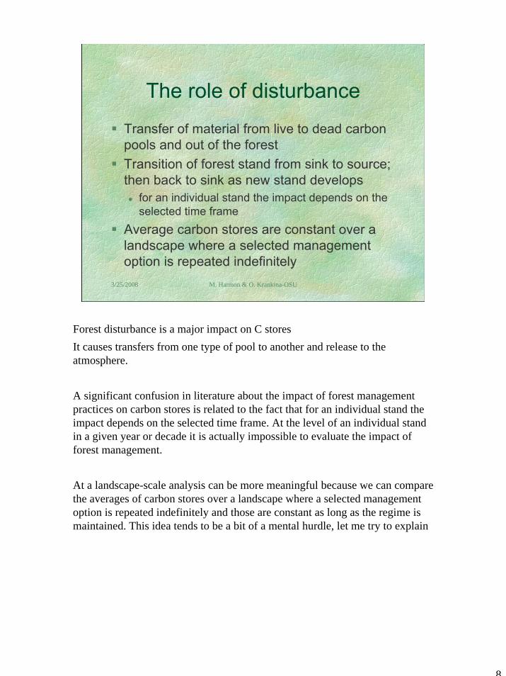
Forest disturbance is a major impact on C storesIt causes transfers from one type of pool to another and release to the atmosphere.

A significant confusion in literature about the impact of forest management practices on carbon stores is related to the fact that for an individual stand the impact depends on the selected time frame. At the level of an individual stand in a given year or decade it is actually impossible to evaluate the impact of forest management.

At a landscape-scale analysis can be more meaningful because we can compare the averages of carbon stores over a landscape where a selected management option is repeated indefinitely and those are constant as long as the regime is maintained. This idea tends to be a bit of a mental hurdle, let me try to explain

9


0

100

200

300

400

500

600

700

800

450 550 650 750 850 950

Time [years]

Car

bon

Sto

re [M

g/ha

]

40 years 60 years80 years 100 years120 years 160 years

Let’s now consider what happens to a stand when we harvest an old-growth forest and put it on a repeating cycle of harvests.

The first cyan line is for a 40 year rotation. We see the stand loses carbon initially, but eventually starts to gain carbon, then it is harvested and cycle starts again. Notice that in time the forest moves around a mean store and that this mean is lower than the old-growth store.

We can look at other intervals between forests. You should notice that as the interval becomes longer the frequency decreases and the amplitude increases. However, you can also see that the mean that the cycle moves around increases as the interval of disturbance increases.

10


0

100

200

300

400

500

600

700

800

450 550 650 750 850 950

Time [years]

Land

scap

e st

ore

(MgC

/ha)

40 years 60 years80 years 100 years120 years 160 years

Landscape translation

We can get a clearer picture if we run the model for a large population of stands within a landscape. This gets rid of all those ups and downs and just shows the mean trend, which by the way is the landscape average of many stands.

Clearly rotation length makes an important difference. One can gain a 50% increase in C stores by extending rotation from 40 to 100 years. And it makes sense – keeping trees growing and accumulating C should lead to more C in live biomass and in other forest C pools as well. But what about forest products? Their output and C store will decline, right? And will lose the benefit of substituting wood for energy intensive products on top of that? Well, we will compare gains and losses later in the presentation.

11


0

100

200

300

400

500

600

700

800

900

1000

WS06 WS07 WS08 WS09

Bio

mas

s (M

g/ha

)

Forest Floor Fine Woody Debris Snag/Stump Logs Understory Live tree

Total Aboveground Biomass

25 years old

100-450 years old

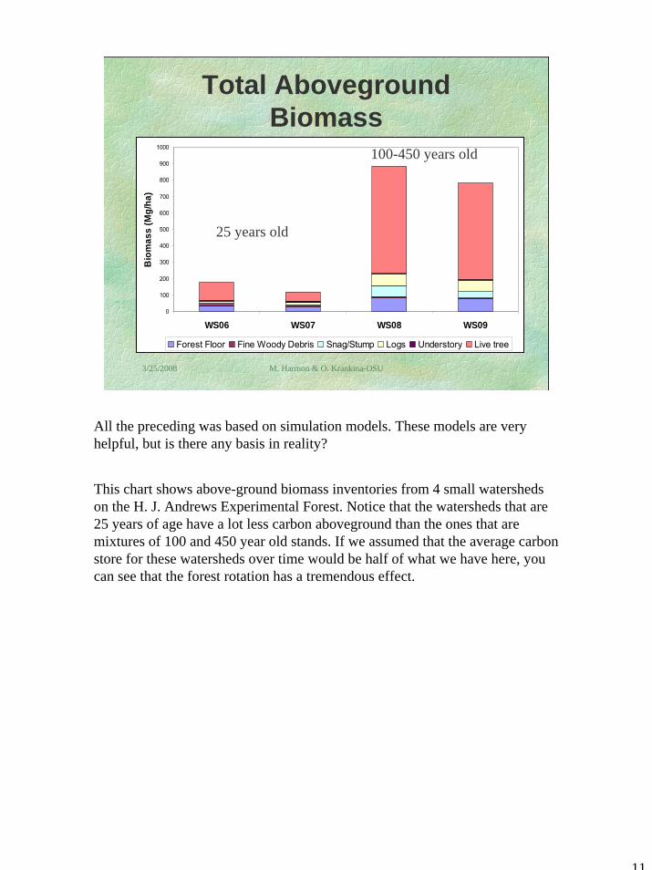
All the preceding was based on simulation models. These models are very helpful, but is there any basis in reality?

This chart shows above-ground biomass inventories from 4 small watersheds on the H. J. Andrews Experimental Forest. Notice that the watersheds that are 25 years of age have a lot less carbon aboveground than the ones that are mixtures of 100 and 450 year old stands. If we assumed that the average carbon store for these watersheds over time would be half of what we have here, you can see that the forest rotation has a tremendous effect.

12


Changes in Live CStocks

Match the Theory of

DisturbanceEffects

Analysis limited to live biomass show interesting differences between private lands and national forests that are consistent with the conceptual model we presented. While all scenarios in both ownerships project increase in C stores the absolute values are vastly different: in NF the current level is over 200 TC/ha and pushes above 300 TC/ha 50 years into the future, on private lands the pattern is similar but the C store values are 3 times lower – this is the scope of long term impact of forest management on C stores.

These observations are completely in line with the predictions of our carbon theory.

13


The Importance of ScalingResults from one time- one place

to another

Statements may be true at one scale and irrelevant at anotherWe need to examine proposals at the appropriate scale of space and timeLandscape levels are probably the best for setting policies

14


0

20

40

60

80

100

120

140

0 50 100 150 200 250 300

Time (years)

Tota

l car

bon

stor

e (M

g C

/ha)

Windthrow50 year timber harvest

-7

-6

-5

-4

-3

-2

-1

0

1

2

0 50 100 150 200 250 300

Time (years)

Cha

nge

in N

et E

cosy

stem

Car

bon

Stor

es (M

g C/h

a/ye

ar)

WindthrowHarvest

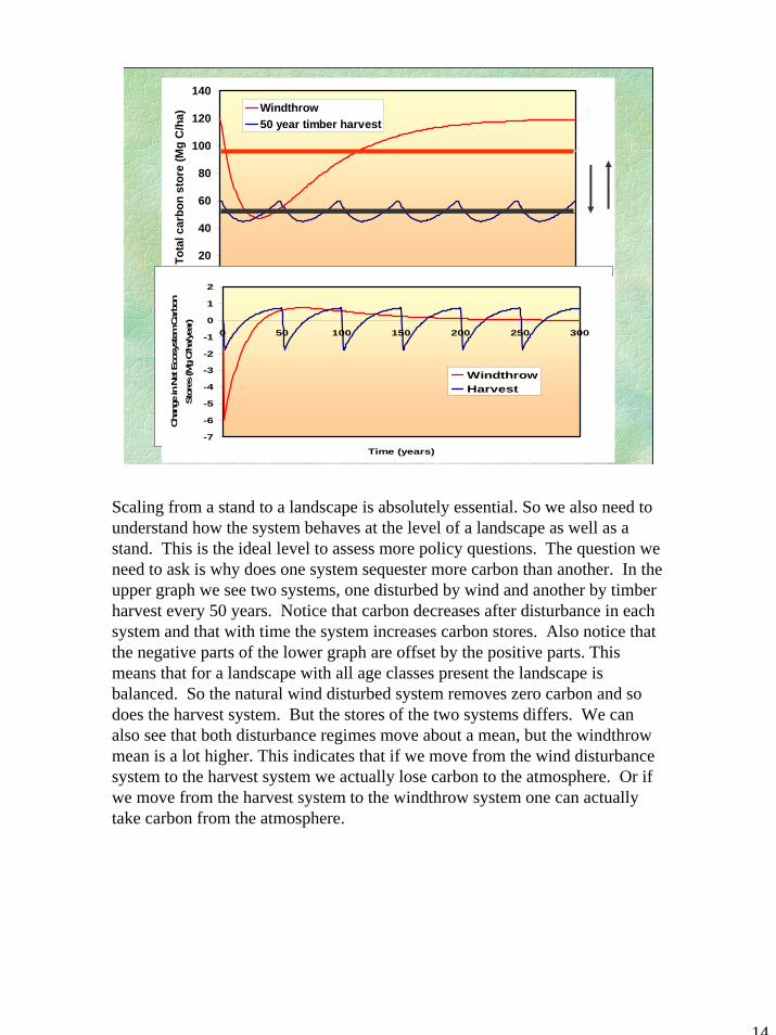
Scaling from a stand to a landscape is absolutely essential. So we also need to understand how the system behaves at the level of a landscape as well as a stand. This is the ideal level to assess more policy questions. The question we need to ask is why does one system sequester more carbon than another. In the upper graph we see two systems, one disturbed by wind and another by timber harvest every 50 years. Notice that carbon decreases after disturbance in each system and that with time the system increases carbon stores. Also notice that the negative parts of the lower graph are offset by the positive parts. This means that for a landscape with all age classes present the landscape is balanced. So the natural wind disturbed system removes zero carbon and so does the harvest system. But the stores of the two systems differs. We can also see that both disturbance regimes move about a mean, but the windthrowmean is a lot higher. This indicates that if we move from the wind disturbance system to the harvest system we actually lose carbon to the atmosphere. Or if we move from the harvest system to the windthrow system one can actually take carbon from the atmosphere.

15


Initial Conditions

Without knowing where you start it is impossible to know how far you have traveled

Mentioning a management system without stating the starting point is meaningless!!!!!!

16


Effect of Initial Conditions: Stand level

0

100

200

300

400

500

600

700

0 50 100 150 200 250 300 350 400 450 500

Time (years)

Tota

l C s

tore

s (M

g/ha

)

initial:agricultureinitial: old-growth

40 year harvest interval

Here is an example of the importance of considering the initial conditions.In both cases we convert from a something to a plantation that is harvested every 40 years. If we start from an agricultural field we gain carbon. If we start from an old-growth forest we lose carbon. Notice that in time the forest is the same regardless of the starting point.

17


Effect of Initial Conditions: Stand to Landscape translation

0

100

200

300

400

500

600

700

0 100 200 300 400 500

Time (years)

Tota

l C s

tore

s (M

g/ha

)

landscapestand


Now let’s look at this from the perspective of not a single stand, but from the perspective of a landscape that is being converted. We can see the stand level line in red. But in a landscape we can’t convert everything at once. In this case it takes 40 years (our harvest interval is 40 years). The blue line shows what happens at the landscape level. As the landscape is converted it loses carbon, but in time it comes into a balance and the stores of carbon don’t change much over time.

18


Effect of Initial conditions:landscape level

0

100

200

300

400

500

600

700

0 50 100 150 200 250 300 350 400 450 500Time (years)

Land

scap

e m

ean

C s

tore

(Mg/

ha) initial: agriculture

initial: old-growth


Here is a view of the effect of initial conditions at the landscape scale. As with the stand level if we convert an agricultural field to a 40-year rotation we gain carbon. If we convert an old-growth forest, then we lose carbon.

19


Forest products sectorRetains carbon in products

Rates of carbon loss through decomposition and combustion are similar to decomposition rates of coarse woody debris on the forest floor

Can contribute to emission reduction in other sectors IF forest products reduce the use of fossil fuels

Gains are cumulative, but may saturateNet carbon gains (compared to no-harvest option) take many decades (or centuries) to begin

Trees are just so incredibly effective in capturing and storing carbon that it is hard for our technology to compete. Because of that most measures reducing timber harvest tend to create some increase in C stores on land.Still we need to consider what happens to harvested carbon.

20


Only 20% of Harvest is Stored

0

200

400

600

800

1000

1200

1400

1600

1800

1900 1920 1940 1960 1980 2000Year

Car

bon

(Tg

C)

CummulativeHarvest

Stores

One often gets the impression that once carbon is harvested all of it ends up as a carbon store. But there are losses in manufacturing and in use.

Based on FORPROD model, which takes in to account those losses, very little of the carbon harvested in the PNW is currently stored. Probably on the order of 20%. And yes this does include the stores in landfills.

21


Forest Products-related partsstand level

40 year harvest:Forest products= 75% Biofuels=12% Substitution 75% of harvest

0

100

200

300

400

500

600

0 50 100 150 200 250 300

Time (years)

Car

bon

"sto

re" (

MgC

/ha)

Forest ProductsBioenergyProduct substitutionProd sub-additionality adjustment

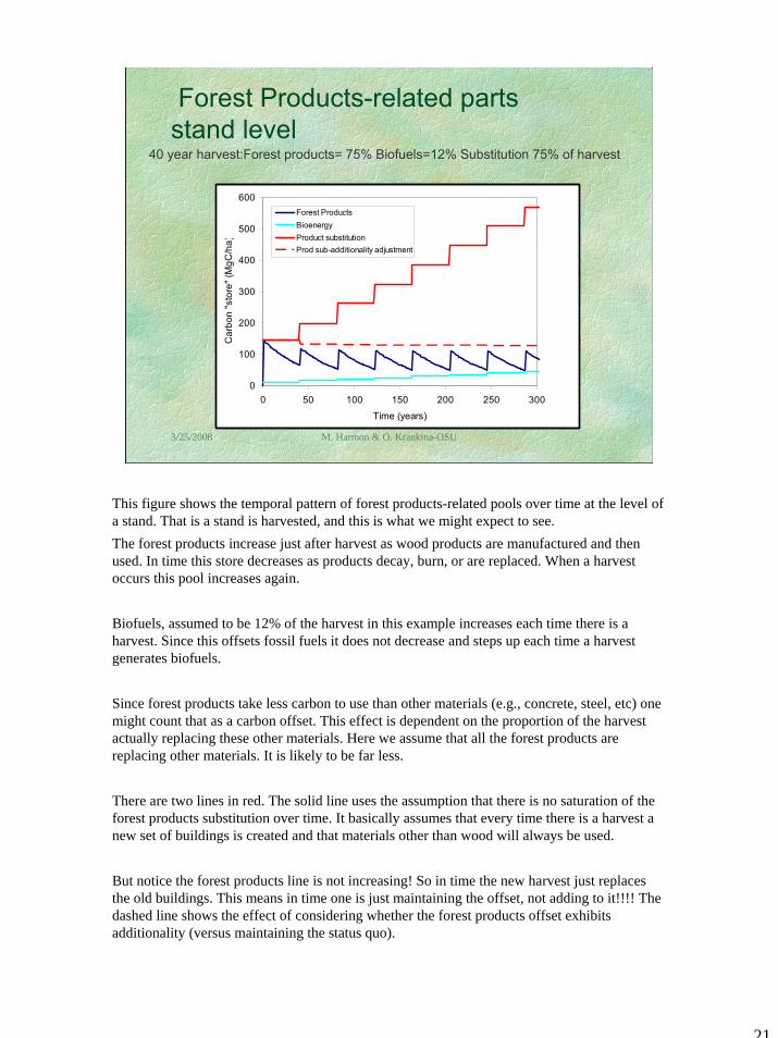
This figure shows the temporal pattern of forest products-related pools over time at the level of a stand. That is a stand is harvested, and this is what we might expect to see. The forest products increase just after harvest as wood products are manufactured and then used. In time this store decreases as products decay, burn, or are replaced. When a harvest occurs this pool increases again.

Biofuels, assumed to be 12% of the harvest in this example increases each time there is a harvest. Since this offsets fossil fuels it does not decrease and steps up each time a harvest generates biofuels.

Since forest products take less carbon to use than other materials (e.g., concrete, steel, etc) one might count that as a carbon offset. This effect is dependent on the proportion of the harvest actually replacing these other materials. Here we assume that all the forest products are replacing other materials. It is likely to be far less.

There are two lines in red. The solid line uses the assumption that there is no saturation of the forest products substitution over time. It basically assumes that every time there is a harvest a new set of buildings is created and that materials other than wood will always be used.

But notice the forest products line is not increasing! So in time the new harvest just replaces the old buildings. This means in time one is just maintaining the offset, not adding to it!!!! The dashed line shows the effect of considering whether the forest products offset exhibits additionality (versus maintaining the status quo).

22


Forest Products-related parts: landscape level

40 year harvest:Forest products= 75% Biofuels=12% Substitution 75% of harvest

0

100

200

300

400

500

600

0 50 100 150 200 250 300

Time (years)

Car

bon

stor

es (M

g/h

a)Forest productsBiofuelsProduct substitutionProd sub-additionality

This is the same graph, but for a landscape. As with the forest carbon figures, this eliminates the irregular spikes and steps caused by disturbance so you can see the general trend.

Again the difference between assuming that forest products offsets saturate or not is quite evident.

Something to consider. If the forest products substitution offset is not tied to the amount of forest products then the longevity of forest products has no effect whatsoever. This is not entirely sensible. It would make sense that the two be related, building wooden structures that last longer should give one a stronger, and longer forest products substitution effect.

23


Stand Dynamics of Forest Products 40 year harvest interval

0

200

400

600

800

1000

1200

0 100 200 300 400 500

Time (years)

Car

bon

stor

es (M

g/ha

)

Ag->Plantation

OG->Plantation

Ag->Plantation-additionalityOG->Plantation-additionality

Now let’s consider what all the forest products-related stores would look like over time for a stand harvested every 40 years.

We see that starting from an agricultural field that forest products-related stores in the blue lines would increase. The amount of the increase is much lower when additionality effects are considered.

For an old-growth conversion the system only gains carbon after the first harvest when the additionality effect is ignored.

24


“Landscape” Dynamics of Forest Products 40 year harvest interval

0

200

400

600

800

1000

1200

0 50 100 150 200 250 300 350 400 450 500Time (years)

Car

bon

stor

es (M

g/ha

)Ag->Plantation

OG->Plantation

Ag->Plantation-additionality

OG->Plantation-additionality

Here is the same set of conversions, but at the landscape scale. This gets rid of all the spikes and steps to reveal the overall trend.

Notice that when additionality of forest product substitution effects is considered that there is an increase associated with biofuels, but it provides a very slow rate of increase

25


Stand Dynamics of Total System 40 year harvest interval

0

200

400

600

800

1000

1200

1400

1600

0 50 100 150 200 250 300 350 400 450 500Time (years)

Car

bon

stor

es (M

g/ha

)Ag->PlantationOG->PlantationAg->Plantation-additionalityOG->Plantation-additionalityOld-growth average

This figure shows what might be happening for the entire forest system (i.e., the forest itself and forest products-related stores) at the stand level.

Two sets of assumptions are presented about forest products substitution effects. In the case of converting an agricultural field to a plantation harvested every 40 years there is a gain in carbon, but the gain is a lot lower and persists for a shorter time when additionality effects are considered. In the case of the old-growth conversion case, the assumptions about additionality become critical. When additionality is considered then the conversion does not every surpass the store in the original forest.

26


“Landscape” Dynamics of Total System 40 year harvest interval

0

200

400

600

800

1000

1200

1400

0 50 100 150 200 250 300 350 400 450 500Time (years)

Car

bon

stor

es (M

g/ha

)Ag->PlantationOG->PlanatationAg->Plantation-additionalityOG->Plantation-additionalityOld-growth average

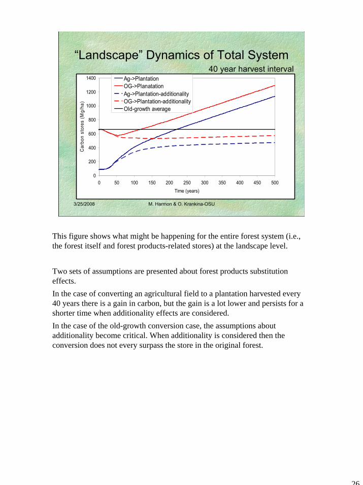
This figure shows what might be happening for the entire forest system (i.e., the forest itself and forest products-related stores) at the landscape level.

Two sets of assumptions are presented about forest products substitution effects. In the case of converting an agricultural field to a plantation harvested every 40 years there is a gain in carbon, but the gain is a lot lower and persists for a shorter time when additionality effects are considered. In the case of the old-growth conversion case, the assumptions about additionality become critical. When additionality is considered then the conversion does not every surpass the store in the original forest.

27


What Happens If?

• We convert slow, decadent, decaying old-growth forests that are not taking up much carbon into:

• Young, thrifty, productive, vibrant forests that are harvested to produce forest products, biofuels, and substitute for concrete, steel, glass etc.

• SOUNDS LIKE A WINNING PLAN TO ME!

The classic proposal to help remove carbon from the atmosphere.

28


Total Carbon Balance-totals- ideal conditions

0

100

200

300

400

500

600

700

800

900

0 50 100 150 200Time (years)

Land

scap

e C

sto

re (M

g/ha

)

old-growth20 years40 years60 years80 years100 years

Forest products= 75% Biofuels=12% Substitution 75% of harvest

This figure shows the total carbon balance (forest and forest products-related) for an old-growth conversion assuming that there is no additionality limitation on forest products substitution. The lines show the effect of converting an old-growth forest to one of these systems. Each line shows a different interval of harvests. For all the intervals considered here, there is a significant lag time before the system stores more carbon than the old-growth system. The shorter the interval the longer the lag, largely due to the fact it decreases the forest stores to a greater degree.

This might be a winning plan, but it would take a lot of time to win.

29


Total Carbon Balance-less than idealForest products= 75% Biofuels=6% Substitution 35% of harvest

0

100

200

300

400

500

600

700

800

0 50 100 150 200Time (years)

Land

scap

e C

sto

re (M

g/ha

)

old-growth20 years40 years60 years80 years100 years

This figure shows the total carbon balance (forest and forest products-related) for an old-growth conversion assuming that there is no additionality limitation on forest products substitution. This is at the landscape scale.The lines show the effect of converting an old-growth forest to one of these systems. Each line shows a different interval of harvests. For all the intervals considered here, there is a significant lag time before the system stores more carbon than the old-growth system. The shorter the interval the longer the lag, largely due to the fact it decreases the forest stores to a greater degree. In this case the assumptions behind the forest products substitution are not as generous, with limits on the amount of biofuels and forest product substitution that can occur. It is half the previous figure. Noticed that none of the harvest intervals gets back to the starting point even after 200 years.

None of these conversions seems like a winning plan.

30


Which might store more C?

• A forest left on it’s own?

• A forest that is frequently harvested?

It is usually assumed that harvesting forests will increase the rate of carbon storage. After all harvested material is put into forest products and the forest regrows etc. And if all the forest products-related stores are considered it would appear that harvesting would increase the carbon sink.On the other hand when we harvest, we only can tap into a small amount of the carbon being stored. And there are losses in manufacturing and use of forest products. Moreover, the harvest causes losses in dead and soil stores.

31


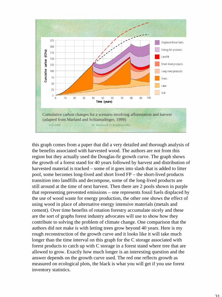
Cumulative carbon changes for a scenario involving afforestation and harvest (adapted from Marland and Schlamadinger, 1999)

this graph comes from a paper that did a very detailed and thorough analysis of the benefits associated with harvested wood. The authors are not from this region but they actually used the Douglas-fir growth curve. The graph shows the growth of a forest stand for 40 years followed by harvest and distribution of harvested material is tracked – some of it goes into slash that is added to litter pool, some becomes long-lived and short lived FP – the short-lived products transition into landfills and decompose, some of the long-lived products are still around at the time of next harvest. Then there are 2 pools shown in purple that representing prevented emissions – one represents fossil fuels displaced by the use of wood waste for energy production, the other one shows the effect of using wood in place of alternative energy intensive materials (metals and cement). Over time benefits of rotation forestry accumulate nicely and these are the sort of graphs forest industry advocates will use to show how they contribute to solving the problem of climate change. One comparison that the authors did not make is with letting trees grow beyond 40 years. Here is my rough reconstruction of the growth curve and it looks like it will take much longer than the time interval on this graph for the C storage associated with forest products to catch up with C storage in a forest stand where tree that are allowed to grow. Exactly how much longer is an interesting question and the answer depends on the growth curve used. The red one reflects growth as measured on ecological plots, the black is what you will get if you use forest inventory statistics.

32


Products Substitution

• Has lags relative to ecosystem• May saturate (in time one is sustaining the

effect not increasing it)• Depends on fraction of harvest going

toward buildings• May decrease if C cost of other materials

comes down

33


Does this mean no timber harvest?

• No, it does not mean timber should not be harvested

• We need to take less more often• OR

• We need to take more less often

• Store increases as proportion removed decreases

• The proportion removed decreases if we take less each time, or take less frequently

34


Partial Harvest of StandsEcosystem & Products Total

0

100

200

300

400

500

600

700

0 50 100 150 200 250

Rotation interval (years)

Car

bon

stor

es (M

g/ha

)

20% aggregated harvest




100% harvest

This figure shows the simulated effects of harvesting Douglas-fir forests at various intervals and of taking different amounts of the live carbon each harvest. The Y-axis shows the mean landscape store in forest and forest products-related carbon. We see that as the interval between harvests increases, the average amount of carbon that can be stored increases. We also see that as the amount we harvest decreases, the system stores more carbon too. We can take less more often, or more less often and get the same amount of carbon stored.

There are a wide range of options to get the same amount of carbon stored. And many of them include some form of harvest.

35


Reduction of carbon emissions from forest fires

at what carbon cost?when?Are there lags?

Fire and Carbon

36


Image Credit: S. Conard, USDA FS

Fire risk reduction in high fire hazard areas

37


Fire and C balance: the scope of the problem

Fire risk in high fire hazard areas0.2-0.3% per year

Fire emissions5 - 15% of carbon on site (for severe fire!)Remaining biomass retains C

Role in regional C balanceCan eliminate all forest sinks in an extreme fire year (e.g. 2002)On average – 5% of C losses from timber harvest

38


D. P. Turner et al. Scaling net ecosystem production and net biome production over a heterogeneous region in the western United States Biogeosciences, 4, 597–612, 2007

The carbon sequestered as NBP, plus accumulation of forest products in slow turnover pools, offset 51% of the annual emissions of fossil fuel CO2 for the state.

39


Fire risk reduction in high fire hazard areas(From “Principles document from the WCI Forestry Sub-committee Stakeholder Group”; February 28, 2008 Draft)

• controlling stem density through thinning• follow up management to minimize ladder

fuel buildup• establishing “high fire hazard areas and/or

stand conditions”• favoring species with higher fire tolerance

40


400 450 500 550 600

020

4060

8010

0

Years

Live

car

bon

stor

es (M

g C

ha-

1)

ControlT15I20T15I35T25I20T25I35T25I50T50I35T50I50

400 450 500 550 600

160

180

200

220

240

Years

Tota

l car

bon

stor

es (M

g C

ha-

1)ControlT15I20T15I35T25I20T25I35T25I50T50I35T50I50

Thinning scenarios and C stores

(live and total)

41

3/25/2008 M. Harmon & O. Krankina-OSU400 450 500 550 600

4050

6070

8090

100

Years

Fuel

s (M

g C

ha-

1)

ControlT15I20T15I35T25I20T25I35T25I50T50I35T50I50

1st thinning

Thinning and fuel loads in Ponderosa Pine forest type

42


400 500 600 700 800 900 1000

050

100

150

200

250

Years

Live

bio

mas

s (M

g C

ha-

1)

400 500 600 700 800 900 1000

050

100

150

200

250

YearsTo

tal c

arbo

n st

ores

(Mg

C h

a-1)

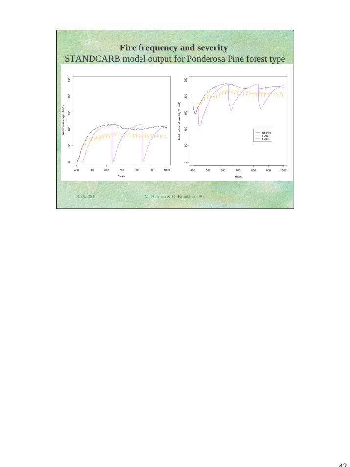
No FireF20LF200H

Fire frequency and severitySTANDCARB model output for Ponderosa Pine forest type

43


Main PointsForests can store carbon (C) –YES! We don’t have a lot to work with, howeverForest C can be permanent, but this decreases as the disturbance frequency and severity increasesForest systems, including products and substitution effects saturateBiofuels are an exceptionOne needs to know starting pointLags between the forest and forest products are significant (decades to centuries)

44


Additionality compared to baseline?Bioenergy

Permanency?Oil engine efficiency

Verifiable?No-till agriculture

Project requirements in forest sector and other sectors

45


Co-benefits of forest offsetsCarbon storage is a new management objective that introduces additional considerations into decision-making

Many strategies that increase C stores in forests also advance other forest management goalsTrade-offs between carbon storage on land and other management objectives are important to recognize

Using synergies to maximize gainsOld-growth conservationWater quality

Recognizing trade-offsWood productsWater quantityFire control

46


47


PrinciplesWe want to change the carbon balance

The balance of anything depends on the inputs versus the outputs

NECB=Cinput-Coutput

In a steady-state inputs and outputs are equalif NECB= 0 then

Cinput=Coutput= kout*storessSo………………………………..

Storess= Cinput/kout

Kout = rate-constant or proportion being lost per time step

Many of the results presented above are surprizing to many. The results may seem counter intuitive. But they are completely in line with basic theory that has been around for decades.

When we consider the landscape average for a disturbance regime we really are talking about a form of a steady-state. That’s because gains in one place are offset by losses in another place. In any steady-state the inputs and the outputs are the same. That’s why it does not appear to change. Actually the rate of change is zero so we can rearrange the equation to have inputs on one side and losses on the other. We can more fully describe the losses as a function of the mass and the rate-constant of loss. The mass is the steady-state mass. So we can rearrange further and set up a simple equation based on the input flux and the proportion of losses.

48


Determining the LossesKout = rate-constant or proportion being lost per time step

kRh=0.02 per year

Kdist= Fdist*Rdist

Fdist frequency of disturbance; 1/interval

Rdist amount removed by disturbance

0.0000

0.0500

0.1000

0.1500

0.2000

0.2500

0.3000

0.3500

0 50 100 150 200Disturbance interval (years)

Loss

rate

-con

stan

t (pe

r yea

r)

Now we need to figure out what controls the proportion of carbon that is lost.

There are two things to consider. First, there are losses associated with decomposition and other heterotrophic processes. This might be viewed as a constant for a landscape.

The other is related to disturbances. Disturbance related losses are controlled by the frequency of the disturbance (Fdist) and the amount removed by a disturbance (Rdist). Note that taking 10% every 10 years is the same as taking 1% per year.

49


Simple Model Predictions

0

50

100

150

200

250

300

0 50 100 150 200Disturbance interval (years)

Stea

dy-s

tate

sto

re (M

g/ha

)

remove all live

remove 1/2 live

no disturbance

This figure shows the theoretical prediction. We can see that as the disturbance interval increases the average amount of carbon stored in a landscape should increase. We also see that as we take less we also have more carbon stored. The trends match that predicted by much more complicated and realistic simulation models. The point is that the underlying mechanism is quite simple.

50


Scaling to a Landscape:100 regularEffect of adding stands to landscape

0

200

400

600

800

1000

1200

1400

0 100 200 300 400

Time (years)

Tota

l C S

tore

s (M

g/ha

)

1 run5 runs10 runs25 runs50 runs100 runs

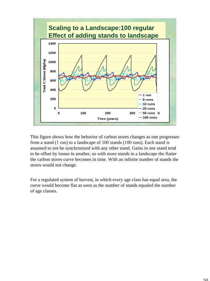
This figure shows how the behavior of carbon stores changes as one progresses from a stand (1 run) to a landscape of 100 stands (100 runs). Each stand is assumed to not be synchronized with any other stand. Gains in one stand tend to be offset by losses in another, so with more stands in a landscape the flatter the carbon stores curve becomes in time. With an infinite number of stands the stores would not change.

For a regulated system of harvest, in which every age class has equal area, the curve would become flat as soon as the number of stands equaled the number of age classes.

51


NECB at Landscape-level

-160

-140

-120

-100

-80

-60

-40

-20

0

20

40

2000 2050 2100 2150 2200

Time (years)

NEP

(Mg/

ha/y

r)

regulated 50natural 50

B

This figure shows two stands over time and the net change in carbon stores. That is the change from one year to the next. The regulated has a disturbance every 50 years. The natural has random intervals of harvest, but the average is 50 years.

52


NECB at Landscape-level

-160

-140

-120

-100

-80

-60

-40

-20

0

20

40

0 50 100 150 200

Time (years)

NEP

(Mg/

ha/y

)

50 nat50 reg

Stan

d le

vel

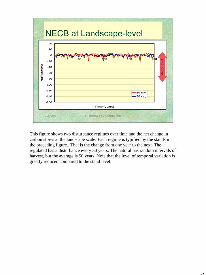
This figure shows two disturbance regimes over time and the net change in carbon stores at the landscape scale. Each regime is typified by the stands in the preceding figure.. That is the change from one year to the next. The regulated has a disturbance every 50 years. The natural has random intervals of harvest, but the average is 50 years. Note that the level of temporal variation is greatly reduced compared to the stand level.

53

3/25/2008 M. Harmon & O. Krankina-OSU435-600 1235-1400

HarvestLiveDeadStable

Trea

tmen

t effe

ct re

lativ

e to

con

trol (

Mg

C h

a-1)

-10

010

2030

40? ?

Near-term and long-term effects of aggressive thinning + fire scenarios: comparison with baseline (fire-no-thinning)

Average C stores on site and total harvest over the first 165 years and the last 165 years.

Documents

Forest Carbon Basics - Our City