Forest Canopy Waves: The Long-Wavelength Component

FOREST CANOPY WAVES: THE LONG-WAVELENGTH COMPONENT

MANUEL PULIDO1 and GEORGE CHIMONAS2,�

1Grupo de Fisica de la Atmosfera, FaMAF, Universidad Nacional de Cordoba, Argentina; 2Schoolof Earth and Atmospheric Sciences, Georgia Institute of Technology, Atlanta, GA 30332-0340,

U.S.A.

(Received in final form 2 January 2001)

Abstract. Air flowing over a forest canopy is examined for instabilities driven by Jeffreys’ dragmechanism. The calculations indicate that the mechanism is generally effective in strong wind con-ditions and extremely effective when the boundary layer supports wave trapping. The instabilityforces the free wind down amongst the trees, creating episodes of stress in the foliage.

Keywords: Canopy waves, Gusts, Instability, Turbulence.

1. Introduction

Flows may have instabilities that grow by modulating frictional stresses, as Jeffreysdemonstrated for water running down a rough inclined channel (Jeffreys, 1925). Asimilar drag mechanism destabilizes the Earth’s surface wind (Chimonas, 1993),while this paper applies the mechanism to the wind over a forest canopy. In aforest, a wave forces the free-air stream down into the trees creating a drag, andthis drag feeds back into the wave – the feedback causes the wave to amplify. Theinstability becomes more effective as the speed of the free wind increases and mosteffective when there is a shallow near-surface wave duct.

This study is intended to demonstrate the new application of Jeffreys’ dragmechanism and generate interest in it as an integral part of boundary-layer dy-namics. At this time the only concise formulation of the mechanism involves along-wavelength approximation, and our results demonstrate that the canopy-draginstability is effective in this limit. However, the long-wave formulation predictsa monotonic increase in growth rate as the wavelength decreases, which is al-most certainly incorrect; thus the scale at which the instability peaks is currentlyunknown, inviting work that treats the smaller scales consistently.

Observations of waves and eddies in a canopy are reviewed by Raupach etal. (1996). The review is mainly concerned with the small-scale structure, andRaupach et al. show that this end of the spectrum obeys Kelvin–Helmholtz scalinglaws. Raupach et al. (1996) also identify a long-wavelength component that mod-ulates the short-wavelength activity, and refer to this long-wavelength component

� Corresponding author: George Chimonas, E-mail: [email protected]

Boundary-Layer Meteorology 100: 209–224, 2001.© 2001 Kluwer Academic Publishers. Printed in the Netherlands.

210 MANUEL PULIDO AND GEORGE CHIMONAS

Figure 1. The structure of the two-layer model. The flow is ducted between rigid plates at z = ±h.

as ‘inactive turbulence’, which is generally visualized in terms of large vortices.However, inactive turbulence includes a wave component – Einaudi and Finnigan(1993) postulate a continuous exchange between waves and turbulence at thesescales – and our study shows that Jeffreys’ mechanism is a very effective source oflong-wavelength boundary-layer waves, and thus a source for the long-wavelengthdisturbances in all their forms. We suspect that Jeffreys’ mechanism also enhancesthe growth of the smaller-scale Kelvin–Helmholtz disturbances, although confirm-ation of this (or its rejection) must await a short-wavelength formulation of themechanism.

2. A Two-Layer Demonstration

The instability is demonstrated with the simplest model that incorporates Jeffreys’mechanism into canopy drag. The undisturbed flow, shown in Figure 1, consists oftwo homogeneous layers of incompressible fluid each filling half the space betweenrigid horizontal plates set 2h apart. The lower layer is at rest and has density ρ1,while the upper layer has horizontal speed U and density ρ2. The lower half of thespace contains trees that create a drag on any flow within them.

FOREST CANOPY WAVES 211

Coordinates are chosen with x parallel to the mean wind and z in the verticaldirection, while t denotes time. A wave with phase speed c and wavenumber k

propagates along the layers causing a vertical displacement η′ of fluid parcels abouttheir mean heights

η′(x, t, t) = η(z) exp ik(ct − x). (1)

The displacement brings the air above into contact with the trees, and the friction-force per unit volume exchanged between wind and foliage is formulated with theaerodynamic law

F(x, z, t) = −ρ(C/h)V|V|, (2)

where V is the air velocity through the foliage and C/h is an effective volume-dragcoefficient (C is a dimensionless number and h, the canopy depth, is set equal tothe depth of the lower layer). The resistance exerted by a canopy is a function ofmany variables, including the aerodynamic drag coefficients of the trunks, branchesand leaves, and the cross sections and volume-densities of these elements (Amiro,1990). The formulation (2) provides the overall friction so the C used here is acombination of the factors presented in Amiro (1990).

As shown in Figure 1, a sub-layer of depth η(0) is forced below z = 0 so thatthe half-cycles with η′(x, 0, t) < 0 are brought within the trees. Then, to first-orderin the wave amplitude, the total friction force acting on a vertical column of unitcross-section drawn through the upper fluid is∫upper−layer fluid

F(x, z, t) dz ={ −x̂ρ(C/h)U 2|η′(x, 0, t)| for η′(x, 0, t) < 0

0 for η′(x, 0, t) > 0,(3)

where x̂ is the unit vector in the direction of the mean wind. Since the lower fluidis at rest there is no first-order drag on it; if the lower fluid contained a mean windit would experience a stabilizing first-order drag (Lee, 1997).

Following the spirit of Jeffreys’ (1925) approach two simplifying approxima-tions are made: the wavelength is taken to be greater than 2πh (so that (kh)2 < 1),and the force (3) is redistributed uniformly over the upper-layer column (presum-ably by turbulence). The phase speed c of the wave then obeys the dispersionrelation (see Appendix A)

c2 + (c − U)2 − g�ρ

ρh − i

CU 2

2kh= 0, (4)

where �ρ = (ρ1 − ρ2) is the density drop between the layers and ρ is the averagedensity. Only the stable stratification �ρ > 0 is considered.

When the drag is omitted the solutions of (4) reduce to the bounded two-layer,long-wavelength, Kelvin–Helmholtz result

c = U

2±√hg �ρ

2ρ− U 2

4. (5)


There is no instability (c is real) if the energy tied up in the stable-stratificationgh�ρ exceeds the kinetic energy 1

2ρU2. But with the drag included (4) always

has an unstable root (imaginary part of c < 0). The limiting condition for Kelvin–Helmholtz waves, gh�ρ/2ρ − U 2/4 = 0, is particularly easy to examine. Thefrictionless solution (5) reduces to a single, non-growing wave propagating at themean speed U/2 of the fluid, while with friction there are two solutions of (4), onethat grows in time and one that decays

c = U

2

(1 ± (1 + i)

√C

2kh

). (6)

The growing mode (the one with the negative imaginary part) travels more slowlythan the mean fluid speed U/2 while the decaying mode is faster. The growingmode has the following properties:

(a) As its wavelength 2π/k increases the wave becomes more retrograde relativeto the mean flow, eventually moving in the opposite direction to the wind. Theinstability then has no critical level. Jeffreys’ water-channel instabilities alsolacked critical levels, and this is a feature that distinguishes drag instabilitiesfrom shear instabilities as the latter always have critical levels.

(b) The wave (1) grows exponentially at the rate −kIm[c], which equalsU/2

√Ck/2h, so the growth rate is zero for infinite wavelength and increases

continuously towards shorter wavelengths. Since the formulation has usedthe long-wavelength approximation (kh)2 < 1 its predictions are alreadyquestionable at (kh)2 = 1 and we do not know where the instabilitymaximizes.

(c) The growth rate increases with the strength of the free wind U . This is ex-pected, since the wind is the sole source of energy. But it also suggeststhat instability and hence gusting should be more common in strong-windconditions.

(d) The growth rate increases with the coefficient C, which emphasizes that fric-tion is creating the instability. Lee and Barr (1998), observed that wave activityin a forest does indeed decrease with leaf-fall and its attendant reduction of C.

A numerical example gives a sense of the strength of these instabilities. The timeτ for a wave to grow by one factor of e is 1/(Imaginary part of ck), so from (b)τ = 2/U

√2h/Ck. Setting U = 5 m s−1, h = 15 m, C = 1.5 (the large end

of observed values) and a wavelength of 100 m (kh ≈ 1) leads to τ = 7 s. Evenwavelengths of 1 kilometre (kh ≈ 0.1) take only 23 s to exponentiate, and thus haveexplosive growth rates. The instability would still be meteorologically significantif factors not considered here reduced growth by an order of magnitude.


Figure 2. The structure of the three-layer model.

3. A Model without the Upper Plate

The finite duct of Section 2 is opened to the overlying atmosphere, the rigid plate isremoved and the free atmosphere is continued upward to mimic a deep, neutrallystratified residual layer, Figure 2. The drag on the atmosphere that results whenthe wave forces the free wind down into the trees is redistributed (presumably byturbulence) over a middle-layer column of thickness l. The dispersion relation forthe wave (1) in this flow is (Appendix A)

c2 + (c − U)2 kh

(1 + kl)− g

�ρ

ρh − i

CU 2

2(1 + kl)= 0. (7)

The long-wavelength approximation (kh)2 < 1 and the shallow-mixing approxim-ation (kh)2 < 1 are both imposed. With (kl)2 � 1 the value of l has no significantinfluence in (7).


As in Section 2 the drag instability is evaluated relative to the Kelvin–Helmholtzinstability. When the drag term is discarded (7) provides the Kelvin–Helmholtzsolutions

c = Ukh

1 + k(l + h)

−√�ρ

2ρ

gh(1 + kl)

1 + k(l + h)+(

khU

1 + k(l + h)

)2

− khU 2

1 + k(1 + h).

(8)

Comparing this with (5) shows that removing the upper plate has reduced the im-portance of the velocity terms in the regime (kh)2 < 1 of the model. Accordingto (8), even a minimal stable density contrast (�ρ > 0) now makes c real at thelonger wavelengths. However, when drag is retained, the dispersion relation (7)always has an unstable solution

c = Ukh

1 + k(l + h)

−√�ρ

2ρ

gh(1 + kl)

1 + k(l + h)+(

khU

1 + k(l + h)

)2

− khU 2

1 + k(l + h)+ i

CU 2

4(1 + kl)

(9)

(with the square root defined to be in the upper-half plane).The instability retains the general properties outlined in Section 2: it is retro-

grade with respect to the mean flow and its growth increases with the strengthof the free wind U and the coefficient C. The growth rate −Im(ck) decreaseswith large wavelength faster than before, but long wavelengths are unstable whereKelvin–Helmholtz theory would have no instabilities.

Direct comparison of the friction contributions in (7) and (4) shows that theupper plate makes the drag instability more effective. This is because removingthe plate adds additional mass to the wave but does not change the net drag force.Reduced growth is most noticeable at the longest wavelengths, as these reside to agreater degree (as Ae−kz) in the fluid that is exposed by removing the plate.

4. Numerical Results

The dispersion relations for c are evaluated for characteristic canopy situations.The coefficient C varies from 0.3 for a typical stand of pines to 1.5 for spruce trees(Amiro, 1990: note that this reference resolves C into more basic factors).


Figure 3. Wave phase speeds in the three-layer model with �ρ = 0, U = 5 m s−1 and h = l = 15 m.

4.1. NO UPPER PLATE, NO DENSITY CONTRAST

The governing equation is (9) with �ρ = 0. Numerical results are given for U =5 m s−1 and h = l = 15 m. Figure 3 shows the phase speeds as a function ofwavelength for Kelvin–Helmholtz waves (C = 0), and then the speeds with thelarge value C = 1.5. Figure 4 plots the time τ for a wave to grow by one factor ofe; note that the friction increases instability above the Kelvin–Helmholtz rate.

4.2. NO UPPER PLATE, STRONG STABLE DENSITY CONTRAST

As in the previous situation U = 5 m s−1 and h = l = 15 m. The governing equationis (9) with �ρ/ρ = 0.02; this degree of stratification, which is within the observedrange (Lee, 1997; Lee et al., 1997), prevents growth of Kelvin–Helmholtz wavesat the longer wavelengths. Figure 5 shows wave phase speeds for three values ofthe canopy friction: C set to 0, 0.3 and 1.5. Figure 6 shows the correspondinggrowth-times τ .


Figure 4. Time for the wave to exponentiate in the three-layer model with �ρ = 0, U = 5 m s−1

and h = l = 15 m.

4.3. AN UPPER PLATE AND A STRONG STABLE DENSITY CONTRAST

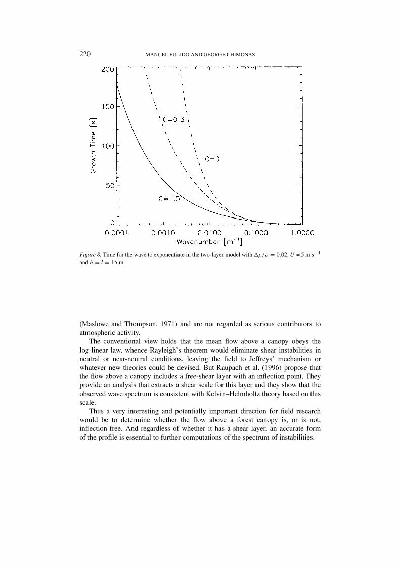
The governing equation is (4) with �ρ/ρ = 0.02 and all the other parameters alsothe same as those used in 4.2 so that one can compare the capped and uncappedcases directly. The results, displayed in Figures 7 and 8, should be contrasted withFigures 5 and 6. The upper plate makes the instabilities an order of magnitude moreeffective.

5. Discussion and Conclusions

Our study indicates that Jeffreys’ drag mechanism can provide useful insights intowaves and eddies in a forest canopy, although the model is much too simple forrealistic predictions of atmospheric behaviour. In this section we summarize thepotential of the drag mechanism, we outline the developments needed to producean acceptable atmospheric model, and we identify field observations that wouldhelp further theoretical development.


Figure 5. Wave phase speeds in the three-layer model with �ρ/ρ = 0.02, U = 5 m s−1 andh = l = 15 m.

5.1. POTENTIAL OF THE DRAG MECHANISM

The long-wavelength behaviour found in this study should carry over into morerealistic models. Thus Figures 4, 6 and 8 show that Jeffreys’ drag mechanism ismore effective than the shear-instability mechanism at the longer wavelengths, abehaviour that can also be deduced from the asymptotic forms of Equations (4) and(7). Moreover, Jeffreys’ mechanism can work when shear instability is suppressedby a too-stable stratification (refer to the text between Equations (5) and (6)), orthe geometry of the wind profile (Section 5.3). However, it is quite possible thatdisturbances develop most readily when the Kelvin–Helmholtz and the Jeffreys’instabilities work together, providing a hybrid that should not be identified as onerather than the other. The suggestion by Lee et al. (1997) that the term ‘canopywaves’ be used to avoid presumptions about the dynamics seems appropriate.

Figures 6 and 8 also illustrate that the instabilities are much more effective whenthey are narrowly confined to the near-earth regions. In the model this was achievedby placing a rigid plate at the top of the boundary layer, and although rigid platesdo not exist in the atmosphere over-reflecting layers can exist and can act just likeperfectly reflecting plates. So complex profiles that provide wave trapping by elev-ated over-reflecting layers or other structures should show more long-wavelength


Figure 6. Time for the wave to exponentiate in the three-layer model with �ρ/ρ = 0.02, U = 5 m s−1

and h = l = 15 m.

gustiness than simple profiles. This enhancement applies equally to drag instabilit-ies and shear instabilities, and it should be observable in the climatology of canopywaves.

A feature of Figures 4, 6 and 8 that is almost certainly incorrect is the ever-increasing effectiveness of the instability as its wavelength decreases. When thesudden jump of the Kelvin-Helmholtz profile is replaced by a continuous transition,the growth rates of the instabilities peak at the scale of the transition region (Milesand Howard, 1964). In addition to this transition scale, the canopy problem involvesthe canopy depth h and the mixing-layer depth l (introduced in Section 3). Thesescales will control the form of the instability at short wavelengths, and will almostcertainly select a wavelength for maximum growth rate.

5.2. COMPLEXITIES THAT MUST BE ADDED TO THE MODEL

The most distressing shortcoming of the model is its use of the long-wavelengthapproximation, and this must be addressed to bring drag theory to a state compar-able with modern shear-instability theory. This may prove difficult, since drag isat root a non-linear, turbulent problem. Jeffreys used an integral method to replacethe complex spatial distribution of turbulent stresses by their net effect – the aero-


Figure 7. Wave phase speeds in the two-layer model with �ρ/ρ = 0.02, U = 5 m s−1 andh = l = 15 m.

dynamic drag at the surface. This provides a brilliant simplification of the problem,but it is not at all obvious how to extend the approach to short-wavelength disturb-ances. The alternative is a fully numerical approach, which we do not contemplateattempting. However, if a suitable linearised formulation can be developed the nextstep will be to contrast instabilities in log-linear wind profiles with instabilities infree-shear wind profiles. Both forms have been postulated for the structure abovea canopy-and they have very different consequences for shear instabilities (Section5.3).

5.3. POINTS FOR FIELD OBSERVATIONS

The structure of the mean boundary-layer flow provides the best clues to theorigin of any waves observed there. The clearest case is provided by the neutrally-stratified state, since this is governed by Rayleigh’s inflection point theorem, whichmay be stated as ‘An inviscid, neutrally stratified flow in which the shear increasesor decreases monotonically does not have any (linearized) shear instabilities’. Theclassical boundary-layer profiles (log and log-linear) all satisfy this condition andare thus immune from simple shear instabilities. Viscosity does allow Tollmein–Schlichting instabilities in uninflected profiles, but these are very slow-growing


Figure 8. Time for the wave to exponentiate in the two-layer model with �ρ/ρ = 0.02, U = 5 m s−1

and h = l = 15 m.

(Maslowe and Thompson, 1971) and are not regarded as serious contributors toatmospheric activity.

The conventional view holds that the mean flow above a canopy obeys thelog-linear law, whence Rayleigh’s theorem would eliminate shear instabilities inneutral or near-neutral conditions, leaving the field to Jeffreys’ mechanism orwhatever new theories could be devised. But Raupach et al. (1996) propose thatthe flow above a canopy includes a free-shear layer with an inflection point. Theyprovide an analysis that extracts a shear scale for this layer and they show that theobserved wave spectrum is consistent with Kelvin–Helmholtz theory based on thisscale.

Thus a very interesting and potentially important direction for field researchwould be to determine whether the flow above a forest canopy is, or is not,inflection-free. And regardless of whether it has a shear layer, an accurate formof the profile is essential to further computations of the spectrum of instabilities.


Acknowledgements

This research was supported in part by grant ATM-9422869 from the NationalScience Foundation and in part by CONICET and FOMEC, sponsors of ManuelPulido’s visit to the Georgia Institute of Technology.

Appendix A: Derivation of the Dispersion Relations

The unperturbed flow V0 of the model is

V0 = x̂V0 ={

x̂U above the canopy layer0 within the canopy layer.

(A1)

The instabilities have the form

{u,w, p, η} = {u′(z),w′(z), p′(z), η′(z)} exp ik(ct − x), (A2)

where {u′, w′} are the x and z components of the perturbation velocity, p′ is theperturbation pressure and η′ is the vertical displacement of the streamlines. Thewaves of interest have periods less than an hour so the derivations given here ignoreCoriolis accelerations from the outset (we have checked for subtle influences ofthe Coriolis terms and have found none). Following Jeffreys’ original study, thelong-wavelength approximation is invoked: u′(z) and p′(z) are set constant withineach layer of the two-layer model and within each of the two lower layers of thethree-layer model.

The perturbed atmosphere is treated as in an ideal, incompressible fluid thatexchanges momentum with the tree canopy through aerodynamic drag. Theincompressibility condition applied to the wave (A2) produces

∂w′

∂z= iku′. (A3)

Within a layer where u′(z) = ulayer is a constant the integration of (A3) leads to

w′(z) = a + (ikulayer)z, (A4)

where the constant a must be determined by a boundary condition.Within each layer the linearized x-component of the momentum equation

reduces to

ρ

(∂

∂t+ V0

∂

∂x

)u′ = −∂p′

∂x+ F′

x (A5)

hence

ρi(c − V0)ku′ = ikp′ + F′

x. (A6)


The term F′x is the wave component of the drag force (2) introduced when the mean

wind (10) is drawn down into the tree canopy. The column integral of the drag forceis given by (3), and the component exp ik(ct − x) is extracted by Fourier theory as∫layer

F′x dz =

{12ρ2(C/h)U

2η′(x, 0, t) for the layer forced down into the canopy0 for all other layers.

(A7)

The result (A7) is only correct for linear theory.Integrating (A6) over the layer-depth L and using (A7) gives the long-

wavelength approximation

ρ2i(c − U)ku2L2 = ikL2p2 + 1

2ρ2(C/h)U

2η(0), (A8)

for the upper layer of the two-layer model (Figure 1, and L2 = h) and the middlelayer of the three-layer model (Figure 2, and L2 = l). There is no drag term in thelowest layer and (A6) gives directly

ρ1cu1 = p1. (A9)

DISPERSION RELATION FOR THE TWO-LAYER MODEL

The two-layer model is bounded by rigid plates at z = ±h, so w′(z) must be zeroat these points and (A4) yields

w′(z) ={iku2(z − h) upper layeriku1(z + h) lower layer.

(A10)

The displacement η = w′(z)/ik(c − V0) must be continuous across the interfaceof the two layers, hence

−hu2

(c − U)= hu1

c. (A11)

The pressure must also be continuous across the displaced interface, so from (A8),(A9) and the hydrostatic condition of the mean state

ρ2(c − U)u2 +[

i

2khρ2(C/h)U

2 − ρ2g

]hu1

c= ρ1cu1 − ρ1g

hu1

c. (A12)

The condition that (A11) and (A12) have a nontrivial solution provides thedispersion relation

(c − U)2 + ρ1

ρ2c2 − (ρ1 − ρ2)

ρ2gh − i

2khCU 2 = 0. (A13)


Since atmospheric inversions are in the regime ρ1 = ρ2 +�ρ with �ρ/ρ2 � 1the densities of the layers can be set equal to their mean except in the differenceterm to give the form (4) presented in the text.

DISPERSION RELATION FOR THE THREE-LAYER MODEL

The three-layer model builds on the two-layer model, replacing the upper platewith an unbounded homogeneous flow. In this uppermost region the disturbance isthe bounded solution

{u,w, p, η} = u3

{1,−i, ρ2(c − U),

−1

(c − U)k

}exp[ik(ct − x) − kz]. (A14)

In the middle layer, which has depth l, (A4) and (A8) become

ρ2i(c − U)ku2l = iklp2 + 12ρ2(C/h)U

2η(0)w′(z) = w′(l) + iku2(z − l).

}(A15)

Continuity of pressure and displacement at z = l relates the fields (A14) and(A15), requiring that

iw′(l)ρ2(c − U) = p2. (A16)

The lowest layer still obeys (A9) and (A10)

ρ1cu1 = p1

w′(z) = iku1(z + h)

}(A17)

and continuity of pressure and displacement at the displaced interface of the lowertwo layers requires

η(0) = w′(l) − iku2l

ik(c − U)= u1h

c(A18)

and

iw′(l)ρ2(c − U) =[ρ1c − h

cg(ρ1 − ρ2)

]u11. (A19)

The condition that (A15) through (A19) have a nontrivial solution provides thedispersion relation. In the approximation that ρ1 = ρ2 + �ρ with �ρ/ρ2 � 1the densities of the layers can be set equal to their mean except in the gravitationalterm to yield the result (7) presented in the text.

References

Amiro, B.: 1990, ‘Drag Coefficients and Turbulence Spectra within Three Boreal Forest Canopies’,Boundary-Layer Meteorol. 52, 227–246.


Chimonas, G.: 1993, ‘Surface-Drag Instabilities in the Atmospheric Boundary Layer’, J. Atmos. Sci.50, 1914–1924.

Einaudi, F. and Finnigan, J. J.: 1993, ‘Wave-Turbulence Dynamics in the Stably Stratified BoundaryLayer’, J. Atmos. Sci. 50, 1841–1864.

Jeffreys, H.: 1925, ‘The Flow of Water in an Inclined Channel of Rectangular Section’, Phil. Mag.49, 793–807.

Lee, X.: 1997, ‘Gravity Waves in a Boreal Forest: A Linear Analysis’, J. Atmos. Sci. 54, 2574–2585.Lee, X. and Barr, A. G.: 1998, ‘Climatology of Gravity Waves in a Forest’, Quart. J. Roy. Meteorol.

Soc. 124, 1403–1419.Lee, X., Neuman, H., Den Hartog, G., Feuntes, J., Black, T., Mickle, R., Yang, P., and Blanken, P.:

1997, ‘Observation of Gravity Waves in a Boreal Forest’, Boundary-Layer Meteorol. 84, 383–398.

Maslowe, S. A. and Thompson, J. M.: 1971, ‘Stability of a Stratified Free Shear Layer’, Phys. Fluids14, 453–458.

Miles, J. W. and Howard, L. N.: 1964, ‘Note on a Heterogeneous Shear Flow’, J. Fluid Mech. 20,331–336.

Raupach, M. R., Finnigan, J. J., and Brunet, Y.: 1996, ‘Coherent Eddies and Turbulence in VegetationCanopies: The Mixing-Layer Analogy’, Boundary-Layer Meteorol. 78, 351–382.

Documents

Forest Canopy Waves: The Long-Wavelength Component