Forensic Investigation of Two Voided Slab Bridges in the … · Forensic Investigation of Two Voided Slab Bridges in the Virginia Department of Transportation’s Richmond District

Forensic Investigation of Two Voided Slab Bridges in the Virginia Department of Transportation’s Richmond District http://www.virginiadot.org/vtrc/main/online_reports/pdf/17-r12.pdf

SOUNDAR S.G. BALAKUMARAN, Ph.D., P.E. Research Scientist Virginia Transportation Research Council BERNARD L. KASSNER, Ph.D., P.E. Research Scientist Virginia Transportation Research Council RICHARD E. WEYERS, Ph.D., P.E. Professor Emeritus Department of Civil and Environmental Engineering Virginia Polytechnic Institute and State University

Final Report VTRC 17-R12

Standard Title Page - Report on Federally Funded Project 1. Report No.: 2. Government Accession No.: 3. Recipient’s Catalog No.: FHWA/VTRC 17-R12 4. Title and Subtitle: 5. Report Date: Forensic Investigation of Two Voided Slab Bridges in the Virginia Department of Transportation’s Richmond District

June 2017 6. Performing Organization Code:

7. Author(s): Soundar S.G. Balakumaran, Ph.D., P.E., Bernard L. Kassner, Ph.D., P.E., and Richard E. Weyers, Ph.D., P.E.

8. Performing Organization Report No.: VTRC 17-R12

9. Performing Organization and Address: Virginia Transportation Research Council 530 Edgemont Road Charlottesville, VA 22903

10. Work Unit No. (TRAIS): 11. Contract or Grant No.: 105175

12. Sponsoring Agencies’ Name and Address: 13. Type of Report and Period Covered: Virginia Department of Transportation 1401 E. Broad Street Richmond, VA 23219

Federal Highway Administration 400 North 8th Street, Room 750 Richmond, VA 23219-4825

Final 14. Sponsoring Agency Code:

15. Supplementary Notes: 16. Abstract: The precast prestressed concrete voided slab structure is a popular bridge design because of its rapid construction and cost savings in terms of eliminating formwork at the jobsite. However, the longitudinal shear transfer mechanism often fails, leading to leakage of salt-laden runoff water between individual beams and increased corrosion of prestressing strands in the beams. Two such slab bridges in Virginia, the Qualla Road Bridge and the Adkins Road Bridge, had delaminations, spalls, and broken prestressing strands. These bridges provided an excellent opportunity to conduct both destructive and non-destructive evaluations of beams after more than 50 years in service. This study was designed to conduct a forensics investigation of voided slab bridges to understand the reasons for deterioration or failure of these bridges and to find ways to identify their deterioration states while the bridges are in service. Tests included material sampling, corrosion and concrete condition assessments, and live load testing of the overall structure. Both structures were found to be in fairly good condition with less corrosion in the strands and a relatively stiffer superstructure than expected. Deck drainage patterns were found to be closely related to the deterioration mechanisms of superstructures with scaling and pop-outs in the outer sides of the fascia beams. Reflective longitudinal cracks formed through the asphalt riding surface allowed chloride-laden water to drain through the joints and wet the top, sides, and bottom of the beams. Accumulated dirt and vegetation growing at the scuppers obstructed the free drainage of runoff, allowing chloride-laden water penetration in these locations. In addition, clear concrete cover thicknesses were generally less than specified at a considerable number of locations, especially at the bottom of the slabs, providing a weaker defense against corrosive chemicals for the strands. However, the analysis showed that the concrete in the Qualla Road Bridge showed moderate chloride ion penetrability in permeability testing and that the Adkins Road Bridge still retained adequate flexural strength to support service loads. The AASHTO-calculated girder distribution factor for interior adjacent members, where there is no vertical displacement at the interface between beams, was found to be sufficient. The results suggest that evaluating bridges considered for replacement with the use of nondestructive techniques, such as determining material and structural conditions, might delay replacement for a number of years and thus free up resources for other needed projects. The study provides a recommendation with regard to how the Virginia Department of Transportation’s Structure and Bridge Division could revise its guidance on design, construction, and maintenance of adjacent member prestressed structures such as voided slabs to address issues identified in this study. 17 Key Words: 18. Distribution Statement: voided slab, shear key, non-destructive evaluation, live load test, in-service performance, corrosion

No restrictions. This document is available to the public through NTIS, Springfield, VA 22161.

19. Security Classif. (of this report): 20. Security Classif. (of this page): 21. No. of Pages: 22. Price: Unclassified Unclassified 61

Form DOT F 1700.7 (8-72) Reproduction of completed page authorized

FINAL REPORT

FORENSIC INVESTIGATION OF TWO VOIDED SLAB BRIDGES IN THE VIRGINIA DEPARTMENT OF TRANSPORTATION’S RICHMOND DISTRICT

Soundar S.G. Balakumaran, Ph.D., P.E. Research Scientist

Virginia Transportation Research Council

Bernard L. Kassner, Ph.D., P.E. Research Scientist

Virginia Transportation Research Council

Richard E. Weyers, Ph.D., P.E. Professor Emeritus

Department of Civil and Environmental Engineering Virginia Polytechnic Institute and State University

In Cooperation with the U.S. Department of Transportation

Federal Highway Administration

Virginia Transportation Research Council (A partnership of the Virginia Department of Transportation

and the University of Virginia since 1948)

Charlottesville, Virginia

June 2017 VTRC 17-R12

ii

DISCLAIMER

The contents of this report reflect the views of the authors, who are responsible for the facts and the accuracy of the data presented herein. The contents do not necessarily reflect the official views or policies of the Virginia Department of Transportation, the Commonwealth Transportation Board, or the Federal Highway Administration. This report does not constitute a standard, specification, or regulation. Any inclusion of manufacturer names, trade names, or trademarks is for identification purposes only and is not to be considered an endorsement.

Copyright 2017 by the Commonwealth of Virginia. All rights reserved.

iii

ABSTRACT

The precast prestressed concrete voided slab structure is a popular bridge design because of its rapid construction and cost savings in terms of eliminating formwork at the jobsite. However, the longitudinal shear transfer mechanism often fails, leading to leakage of salt-laden runoff water between individual beams and increased corrosion of prestressing strands in the beams.

Two such slab bridges in Virginia, the Qualla Road Bridge and the Adkins Road Bridge,

had delaminations, spalls, and broken prestressing strands. These bridges provided an excellent opportunity to conduct both destructive and non-destructive evaluations of beams after more than 50 years in service. This study was designed to conduct a forensics investigation of voided slab bridges to understand the reasons for deterioration or failure of these bridges and to find ways to identify their deterioration states while the bridges are in service.

Tests included material sampling, corrosion and concrete condition assessments, and live

load testing of the overall structure. Both structures were found to be in fairly good condition with less corrosion in the strands and a relatively stiffer superstructure than expected.

Deck drainage patterns were found to be closely related to the deterioration mechanisms of superstructures with scaling and pop-outs in the outer sides of the fascia beams. Reflective longitudinal cracks formed through the asphalt riding surface allowed chloride-laden water to drain through the joints and wet the top, sides, and bottom of the beams. Accumulated dirt and vegetation growing at the scuppers obstructed the free drainage of runoff, allowing chloride-laden water penetration in these locations. In addition, clear concrete cover thicknesses were generally less than specified at a considerable number of locations, especially at the bottom of the slabs, providing a weaker defense against corrosive chemicals for the strands. However, the analysis showed that the concrete in the Qualla Road Bridge showed moderate chloride ion penetrability in permeability testing and that the Adkins Road Bridge still retained adequate flexural strength to support service loads. The AASHTO-calculated girder distribution factor for interior adjacent members, where there is no vertical displacement at the interface between beams, was found to be sufficient.

The results suggest that evaluating bridges considered for replacement with the use of nondestructive techniques, such as determining material and structural conditions, might delay replacement for a number of years and thus free up resources for other needed projects. The study provides a recommendation with regard to how the Virginia Department of Transportation’s Structure and Bridge Division could revise its guidance on design, construction, and maintenance of adjacent member prestressed structures such as voided slabs to address issues identified in this study.

1

FINAL REPORT

FORENSIC INVESTIGATION OF TWO VOIDED SLAB BRIDGES IN THE VIRGINIA DEPARTMENT OF TRANSPORTATION’S RICHMOND DISTRICT

Soundar S.G. Balakumaran, Ph.D., P.E.

Research Scientist Virginia Transportation Research Council

Bernard L. Kassner, Ph.D., P.E.

Research Scientist Virginia Transportation Research Council

Richard E. Weyers, Ph.D., P.E.

Professor Emeritus Department of Civil and Environmental Engineering

Virginia Polytechnic Institute and State University

INTRODUCTION

Background

Voided adjacent slab bridges are built by placing narrow precast slabs side by side and

connecting them with longitudinal shear keys and transverse post-tensioning ties for the structure to act monolithically. The slabs contain voids to reduce the self-weight of the superstructure. The top of the voided slabs typically act as the deck for vehicular traffic, thus eliminating the costs and time involved with formwork for the deck, although a wearing surface may be applied. The rapid construction time also helps to minimize interruption to traffic in cases of bridge or superstructure replacement projects.

Voided slabs also have a much shallower profile relative to bridges composed of

AASHTO (American Association of State Highway and Transportation Officials) prestressed concrete girder or steel girder types with concrete decks with a similar span. Therefore, these bridges may provide greater vertical clearance for vehicular traffic or hydraulic flow underneath the bridge (Virginia Department of Transportation, 2014). Further, the continuous (flat) bottom of the superstructure helps to prevent debris from being caught underneath the bridge during high-water events, thus avoiding blockage of the stream flow and the need for maintenance crews to clear obstructions after the water has subsided.

Figure 1 shows a typical section view of a voided slab superstructure. These types of

structures typically have some type of wearing surface placed on top of the beams, and that wearing surface is usually asphalt. In Virginia, however, bridges on routes that have an average daily traffic (ADT) exceeding 4,000 vehicles per day are required to have a concrete deck. Table 1 reflects VDOT’s general policy for overlay type selection for voided adjacent slab bridges based on the traffic to be carried. In addition, the number of transverse post-tensioned tendons can vary depending on the depth and span of the beams.

2

Figure 1. Typical Cross Section of Voided Slab Structure

Table 1. Standard Overlays for a Given Average Daily Traffic (ADT) and Average Daily Truck Traffic

(ADTT) on Adjacent Voided Slab Bridgesa Design Year ADT ADTT Deck Overlay ≤4,000 ≤100 Asphalt overlay >4,000 100 < ADTT ≤ 200 5-in-thick concrete deck with single layer of reinforcement >4,000 >200 7.5-in-thick concrete deck with two layers of reinforcement

a Virginia Department of Transportation, 2014. There are certain disadvantages with this type of bridge, which can detract from the aforementioned advantages. In particular, when the longitudinal shear keys fail, which is reported to occur frequently in service, the joints begin to leak. Runoff water from the deck carrying deicing salts then diffuses to the sides and bottom of the voided slabs, where the concrete cover is shallower. The shallower cover provides less resistance to penetration of salt contaminants through the concrete to the steel and results in a shorter time before corrosion begins to deteriorate the longitudinal prestressing reinforcement, which is the primary tension-carrying component of the prestressed composite beams. Moreover, post-tensioning ties start corroding with the failure of shear keys. Such deterioration can significantly reduce the load-carrying capacity of the structure and can pose a safety problem for traffic over time.

As of June 2014, the Virginia Department of Transportation (VDOT) had 320 prestressed concrete slab bridges, roughly 2.5% of the bridge inventory. Of these, about 7% had a superstructure rating of 4 or 5, meaning fair to poor condition based on National Bridge Inventory visual inspection and engineering analysis. Two bridges with slab superstructures in VDOT’s Richmond District were being replaced for poor superstructure condition: the Qualla Road Bridge and the Adkins Road Bridge. The Qualla Road Bridge (Federal Structure No. 5302; Virginia Structure No. 0206138) was constructed in 1960 and carried Route 653 over Swift Creek in Chesterfield County. This three-span, voided slab structure spanned 146.1 ft and was 24 ft wide (curb to curb). Each span was 48 ft long with standard PSS-21-36 adjacent prestressed concrete voided slabs reinforced with 3/8-in Grade 250 stress-relieved strand. There was an asphalt overlay without a water-resistant membrane on top of the slabs. Figure 2 shows drawings of the general layout of the bridge.

3

Figure 2. Layout of Qualla Road Bridge: (a) Elevation, (b) Plan, and (c) Cross-Section Views

Bridge inspectors reported a number of issues for the bridge during their routine safety

inspection in 2013, including holes on the side of two fascia beams in Spans 1 and 2, delaminations and hairline cracks on the soffit, scaling on upstream beams, failing longitudinal beam joint concrete, and high flexural deflection on certain beams. The bridge, which carried an ADT of 8,197 vehicles per day, 1% of which was trucks, was immediately posted with a 4-ton load limit after the inspection. Owing to the high volume of traffic and an 8-mile detour distance, the bridge was replaced soon after the inspection.

The Adkins Road Bridge (Federal Structure No. 4815; Virginia Structure No. 0186903)

was constructed in 1959 and carried Route 618 over the Chickahominy River at the Charles City County / Kent County line. Measuring 207.75 ft long and 24.1 ft wide (curb to curb), the five-span structure had a 7-degree horizontal curve and a 5.5-degree superelevation. The spans were either 40.75 ft or 41.5 ft long, with PSS-21-26 standard adjacent prestressed concrete voided

4

slabs as the primary load-carrying components. The prestressing reinforcement was 3/8-in Grade 250 stress-relieved strand. This structure also had an asphalt overlay, but without a waterproofing membrane. Figure 3 shows drawings of the general layout of the bridge. This bridge carried an ADT of 1,119 vehicles per day, of which 2% was trucks. Fully corroded prestressed strands, delaminations on the beam soffit, and scaling on the beam sides were noted during the August 2011 bridge safety inspection. While underneath the bridge during the subsequent inspection in 2013, the inspectors heard a loud noise that was possibly attributable to wire breakage in a prestressing strand. As a result, the bridge was immediately closed to traffic until the superstructure could be replaced, even though the closure resulted in a 10-mile detour.

Figure 3. Layout of Adkins Road Bridge: (a) Elevation, (b) Plan, and (c) Cross-Section Views

Problem Statement

As VDOT engineers continue to design voided slab bridges as new construction or replacement structures for existing bridges, there is a need to conduct forensic investigations to understand the reasons for deterioration or failure of these bridges and to find ways to identify their deterioration states while the bridges are in service, since oftentimes such damage is not readily apparent.

5

PURPOSE AND SCOPE

The purpose of this study was to conduct forensic investigations of voided slab bridges to understand the reasons for deterioration or failure of these bridges and to find ways to identify their deterioration states while the bridges are still in service.

The objectives of the study were as follows: • Understand the reasons for deterioration of the voided slab structures.

• Analyze the residual load-carrying capacity of the deteriorated voided slab structures.

• Identify a non-destructive evaluation (NDE) method(s) for evaluating the condition of

such a bridge in situ to extend the service life of this type of structure. The scope of the study included two voided adjacent slab bridges in VDOT’s Richmond

District that have been in service for more than 50 years and were being replaced: the Qualla Road Bridge and the Adkins Road Bridge. Delaminations, spalls, and severely corroded prestressing strands had been identified on the bottom of both bridge superstructures. The structures were studied through material sampling, NDE methods, and live load testing.

The particular questions asked in this investigation were as follows:

• What is the condition of the lateral post-tensioning ties? How much, if any, section loss is there?

• What is the condition of the top slab of these voided slab structures? Are there any delaminations or spalls? How much corrosion and chloride is present in the top of the box beams?

• What is the chloride profile in the concrete, as a function both vertically down the beam and horizontally across the beam?

• How much corrosion activity is occurring in the prestressing strands, and what is the potential for future corrosion?

• What is the in situ performance of these structures after more than 50 years of service?

METHODS

Overview To answer the study questions, five tasks were performed:

6

1. Conduct a pre-demolition visual assessment of the structure.

2. Conduct in situ NDEs of the structure to assess the potential for corrosion of the prestressing strands.

3. Conduct load testing of the bridge.

4. Conduct additional NDEs of the structure at a storage facility.

5. Conduct a destructive evaluation of the structure at the storage facility to assess the amount of chlorides present in the beams and the ability for more chlorides to penetrate through the concrete to the prestressing strands.

Not every type of evaluation was used on both bridges. Specifically, no load test was conducted for the Qualla Road Bridge because of the rapid nature of the replacement schedule necessary to meet traffic demands. On the other hand, the Adkins Road Bridge remained in place for some time, so access to the sides of the beams at the time of testing was impossible and attempting to conduct a forensic investigation of the bottom of the members in place was exceedingly difficult.

Qualla Road Bridge Over Swift Creek Visual Assessment

Visual assessments are similar to the work carried out by bridge safety inspectors, with the exception of extensive soundings to detect concrete delaminations. The assessments give an updated condition report and include notes about such factors as rainwater runoff flow, drainage conditions, and locations that are susceptible to chloride-laden water.

NDE

Ideally, NDE is conducted in situ prior to any demolition of the structure. The reason is that a number of changes can occur once a structural member is removed from its environment. One particular change that could occur during bridge demolition is the change in an area that is currently delaminated, as mechanical disturbance will cause cracks to propagate. Sections of delaminated concrete may spall during beam removal, therefore altering the end-of-service condition. Further, the moisture profile of the concrete and degree of corrosion damage can change if there is a large enough time lag between the slab removal and when the measurements can be made at a storage facility.

Unfortunately, because of the need to re-open the affected roadway, the voided slabs in

the Qualla Road Bridge were replaced before the research team was able to conduct an extensive in-place NDE assessment of the structural members. Nevertheless, the researchers thought that a good deal of information could be obtained after several of the beams were transported to a temporary storage location. VDOT has used NDE techniques in many applications, such as a

7

forensics study on Route 646 (Aden Road) over Cedar Run in Prince William County. The particular NDE methods used in this study included ground penetrating radar (GPR) and a magnetic pachometer survey for reinforcement and feature location; electrical continuity of reinforcement; electrochemical half-cell potential mapping; four-point electrical resistivity of concrete; linear polarization tests to estimate corrosion rates; and infrared (IR) thermography for damage detection.

For the Qualla Road Bridge, three beams, shown in Figure 4, were selected for NDE. One beam was an exterior beam containing large holes on the exterior face (Beam 1, Span A); these holes had exposed prestressing strand and opened into one of the preformed, cylindrical voids. A second member, Beam 6, Span A, had been reported to have excessive mid-span deflections. The third beam was adjacent to an exterior beam but showed no external damage (Beam 8, Span B). The beams were shipped from the bridge site to the temporary storage location and inverted for ease of access to the tension face of the beams.

For each beam, there were four cross-sectional planes distributed along the beams selected for measurements. At each cross section, there were five sample locations: one on each side of the beam and three on the bottom. Thus, there were 20 test locations on each of the three beams. Figure 5 illustrates the test locations. GPR equipment was used to locate the strands. A magnetic pachometer was used to measure the cover depths at five strand locations along each of four longitudinal cross sections at 4 ft, 18 ft, 30 ft, and 44 ft of the 48-ft-long beams, although this device was unreliable when testing strands spaced 2 in center to center or closer. Electrical continuity was tested for each of the beams among three locations, two near longitudinal extremes at the bottom and one at the side, before half-cell potentials were measured. Half-cell potentials were collected every 2 ft throughout the length of the beams on five strands: three on the bottom and one from each side, as shown in Figure 5, in accordance with ASTM C876, Standard Test Method for Corrosion Potentials of Uncoated Reinforcing Steel in Concrete. However, if a beam was deemed electrically non-continuous, the half-cell test was conducted only on those strands that were directly accessible for electrical contact.

Figure 4. Beams From Qualla Road Bridge Selected for Non-Destructive Evaluation

8

Figure 5. Test Locations on Voided Slab of Qualla Road Bridge

Destructive Evaluation

After the NDE of Qualla Road Bridge was completed, destructive testing was conducted to investigate further the poor condition of the bridges. Essentially, the destructive evaluation involved taking 2-in-diameter cores for determining the chloride content profile through the depth of the concrete and extracting 4-in-diameter cores to assess the ability of chlorides to permeate through the concrete. The 2-in-diameter cores were cut orthogonal to and down to the level of the prestressing strands from both the sides and bottom of the beams.

The cores were sliced in the laboratory at 3/8-in intervals to obtain a sufficient quantity of

powdered concrete for titration, at least 10 g, in accordance with ASTM C1152, Standard Test Method for Acid-Soluble Chloride in Mortar and Concrete (ASTM, 2012a). The 4-in cores for the permeability tests were taken from the sides of the beams above the level of the prestressing strands so as to obtain a sample that was thick enough without hitting of the strands.

These samples were prepared and evaluated in accordance with ASTM C1202, Standard

Test Method for Electrical Indication of Concrete’s Ability to Resist Chloride Ion Penetration (ASTM, 2012b). In order to extract the samples for destructive evaluation, the three Qualla Road Bridge beams were transported to VDOT’s Pocahontas Area Headquarters and were placed upside down so that the bottom and two sides of each beam were accessible. Figure 6 shows the beams in the VDOT yard and the coring process.

Figure 6. Beams of Qualla Road Bridge Placed Upside Down in VDOT Yard

9

Adkins Road Bridge Over the Chickahominy River NDE

All of the beams in the Adkins Road Bridge were assessed using the same NDE techniques as described for the Qualla Road Bridge with the exception of IR thermography. IR thermography was not attempted with this structure because of the time of day the researchers were at the bridge site. Optimal conditions for using this technology entail the person conducting the test being at the bridge near first light or at sunset when the differences in the change in temperature of the object relative to the change in air temperature are most apparent. Load Testing

The second phase of the evaluation involved load testing the structure using a vehicle with a known load placed at specific positions transversely across the bridge. The measurements taken during this test can be compared to the predicted responses calculated by assuming material and geometry properties of the structure. Load testing is a common method of assessing the structural capacity of a bridge and has been done in Virginia on smaller structures such as the Bohon Hollow Road Bridge over the Roanoke River as well as on large signature structures such as the Varina-Enon Bridge.

Instrumentation

Figure 7 shows the locations of the various instruments used during the load test. With the exception of the deflectometers, all instruments were manufactured by Bridge Diagnostics, Inc. (BDI).

Strain Gauges. The longitudinal strain gauges were reusable, surface-mounted BDI

ST350 Intelligent strain transducers, which had a 3-in gauge length and an accuracy of ±2% with a strain range of ±2,000 µε. Because the concrete girders were precast sections, no gauge extensions were needed for taking strain measurements of the concrete. All ST350 gauges placed on the girders were located at mid-width of the bottom of the beams. The strain gauges placed at mid-span were designed to capture the maximum strain in the concrete; the strain gauges placed at the quarter-spans in Beams 3 and 4 served two purposes. The first was to compare strains between the two quarter-points for each beam. The second was to compare strains in adjacent beams at the quarter-span closer to Bent 3, where this quarter-point for Beam 4 is near the location where broken prestressing strands were visible, as shown in Figure 8.

10

Figure 7. Instrumentation Plan for Live Load Test of Adkins Road Bridge. LVDT = linear variable

differential transformer.

Figure 8. Spalled Concrete and Corroded Prestressing Strands in Beam 4 of Span 3, Near the Quarter-Point Closest to Bent 3, of Adkins Road Bridge

Although no soundings (i.e., chain drag or hammer survey) were conducted prior to load testing, there were no visible cracks or spalls on Beam 3. Unfortunately, the spall with exposed and broken prestressing strand in Beam 5 was not discovered by the research team until the time of instrumentation because of the lack of access over the water during the initial scoping. Thus, no plans were made to instrument this portion of the bridge and there were no additional instruments available to monitor this location.

11

Although the barrier rails were constructed of cast-in-place concrete, the researchers applied the same type of BDI strain transducers without gauge extensions in an attempt to assess the stiffness provided by the parapets. The two gauges placed on the upstream barrier were located on the top of the curb and the bottom of the face of the top rail, respectively. The location of the gauge on the rail was slightly different from what was originally planned in Figure 7 because of the condition of the concrete at the top of the railing. All of the strain gauges were attached using rapid-setting adhesive applied to the concrete surface.

Linear Variable Differential Transformers. Eight linear variable differential transformers (LVDTs) were set up to measure differential movement between two sets of adjacent voided slabs. Each LVDT had a range of ±1 in with a maximum linearity error of ±0.5% of full scale. Each LVDT used to measure the differential vertical displacement was attached to an arm of a wooden jig that was affixed to one of the slabs, with the arm extending across the joint to the adjacent slab. The LVDT was held in place with a hose clamp such that the LVDT plunger was perpendicular to the bottom surface. At the same location as the vertical differential deflection measurement, a second LVDT was attached parallel to the bottom surface of the adjacent slab using special clamps provided by BDI. The plunger for this horizontal LVDT rested against the wooden jig for the vertical LVDT. All plungers were set approximately at the middle of the displacement range. The LVDT locations at mid-span were selected for two reasons. The first was to compare movement in a longitudinal joint adjacent to an exterior girder, Joint 1 between Beams 1 and 2, to movement in a longitudinal joint for a pair of interior girders, Joint 7 between Beams 7 and 8. The second was to contrast a joint in relatively poor condition (on the upstream side of the bridge) with a joint that appeared to be in relatively good condition (closer to the downstream side of the bridge). The remaining LVDTs were placed at the quarter-points of Joint 1, as a comparison of differential movements between those two points of the span and the mid-span.

Deflection Measurements. Separate from the differential displacement between two adjacent beams, six beams were instrumented with devices to measure their deflection relative to a ground reference during the load test. Five of the devices were a type of homemade device consisting of a base plate used to secure the device to the beam and a cantilever arm that was pre-deflected about 1 in prior to testing. The pre-deflection was sustained by wires strung to weights anchored in the river bed to serve as an elevation reference. Both pieces of each deflectometer were made of aluminum, and a full-bridge layout of foil resistance strain gauges affixed to the cantilever arm near the base plate measured the strain in the cantilever as it was deflected. As the bridge beams deflected under load, the pre-deflected cantilevers relaxed and a change in strain was recorded. The deflectometers were calibrated in the laboratory prior to performance of the field test and were accurate to 0.005 in when the deflectometer was pre-deflected between 0.5 in and 1 in. Unfortunately, there was an insufficient number of deflectometers with sufficient accuracy available for the load test. Thus, Beam 9 was instrumented with a BDI-supplied wire potentiometer, the accuracy of which (±0.002 in) was verified in the laboratory.

All six deflection devices were placed at mid-width of a given beam but just a few inches off mid-span so as to avoid interfering with the longitudinal strain gauges. The deflectometers were pre-deflected down from the bottom of the beam about 1 in through the use of piano wire

12

extending down to the surface. The wire was anchored by 6 in by 12 in concrete cylinders sitting at the bottom of the river bed. Because the length of wire remained virtually unchanged during testing, the distance between the deflectometer’s arm and the beam decreased as the beam deflected while a load truck traversed the span. This change in distance was the measured amount of beam deflection during testing. The same principle applied to the wire potentiometer with the exception that the wire was extended out of the potentiometer base about 2.5 in.

Tiltmeters. The last type of sensor installed on the bridge was a tiltmeter, which measured the rotation of Beam 4 near the piers. Two devices were located at mid-width of the beam, each as close as practical to the opposite ends of the beam. In the case of the tiltmeter adjacent to Bent 2, that longitudinal distance was about 2 in from the face of the pier. However, the tiltmeter located adjacent to Bent 3 was about 5 in from the face of the pier because of the rough surface on the bottom of the beam making it difficult to stick the tiltmeter any closer to the end of the beam. Both tiltmeters had a range of -10 degrees to +10 degrees and an accuracy of 2% of full scale.

Data Acquisition. All instruments were hard-wired to one of BDI’s STS-Wi-Fi nodes attached to the underside of the bridge and located within 15 ft of each device. The nodes then wirelessly transmitted the information to the STS-Wi-Fi Mobile Base Station, which was located on the ground within the line of sight of each node. From the base station, the data were again relayed wirelessly to a laptop computer, where the data were stored for post-processing. Each instrument was sampled and recorded at a rate of 25 Hz. The BDI system also included a laser-based counter that was attached to the wheel well of the truck, with a reflective target attached to the wheel. As the wheel rotated and the attached reflector passed the laser, the system would record a full revolution of the wheel. Prior to the use of a given truck, the distance traveled for one complete revolution of the wheel was measured and recorded. Thus, the counter system helped to determine the speed as well as the longitudinal location of the truck throughout a given load test. Load Trucks

Typical VDOT dump trucks served as the live load traveling across the bridge. Three separate trucks were used for the tests, each with three axles (a front steering axle and two rear tandem axles). The truck designated “Empty” (hereinafter empty truck) had no stone placed in the load bed; the truck designated “Half” (hereinafter half truck) had about one-half of its load bed filled with stone; and the truck designated “Full” (hereinafter full truck) was fully loaded but limited to the weight that the district bridge engineer felt comfortable with placing on the bridge. Actual axle dimensions and weights are given in Figure 9. The axle weights were measured by the Virginia Department of Motor Vehicles using enforcement-grade portable truck weigh scales on the day of the load test.

13

Figure 9. Axle Dimensions and Weights for the Three Load Trucks Used During Live Load Testing of Adkins Road Bridge Load Cases

Figure 10 shows the various orientations for all three trucks for all six load cases (LCs). LC 1 and LC 2 were symmetrical to LC 3 and LC 4 with respect to the centerline of the bridge. The purpose for the loading symmetry was to test beams and joints that appeared to be in relatively poor condition (LC 3 and LC 4) with those that were in better condition (LC 1 and LC 2). The trucks for LC 1 and LC 4 were positioned such that one wheel line was centered over the longitudinal joint between the exterior and first interior beams. On the other hand, the trucks for LC 2 and LC 3 had one wheel line centered over the first interior beam. The purpose of positioning the truck over the longitudinal joint was to maximize the stress on the joint, whereas the reason for centering the wheel line over the first interior beam was to assess the joint’s ability to transfer load to the exterior beam. The remaining two LCs were designed to assess the strength of Beam 4, as Beam 4 was the one beam that clearly had severely corroded prestressing strands. In addition, although Beam 5 did have exposed and broken strands closer to the opposite pier relative to the spalled section in Beam 4, the research team was unable to observe that location prior to instrumenting the bridge. Thus, the trucks for LC 5 had one wheel line centered over Beam 3 (with the overall truck centered over Beam 4) and the trucks for LC 6 had a wheel line centered over Beam 4 (with the truck centered over Beam 5).

14

Figure 10. Various Orientations of Load Vehicle for Live Load Testing of Adkins Road Bridge

Testing Procedure There was only one load truck on the bridge during any given test. Because of the geometry of the bridge and the traffic barricades placed at both ends, all tests were conducted with the truck traveling at quasi-static speed, i.e., about 2 mph. Each test started with the truck parked on Span 2 and was completed once the vehicle was completely off Span 3 and on Span 4. One member of the research team guided the truck driver throughout each test to ensure that the designated wheel line remained centered on the desired path. Because of instrumentation taking longer than anticipated, there was not enough time to conduct each combination of truck weight and orientation through three repetitions, as desired. Nevertheless, each test was conducted a minimum of two times, with additional runs conducted when there was uncertainty about the instrumentation being properly zeroed prior to the start of a given run. Destructive Evaluation

The district bridge engineer opted to delay reconstruction of the closed Adkins Road Bridge because the ADT on that route was relatively low. Therefore, the voided slabs from the Adkins Road Bridge were not removed from the site around the time of the investigation. Thus, obtaining samples from the bottom of those beams would have required working upside down over water, which was prohibitively difficult. Further, concrete cores would have been retrieved only from the bottom of the beams, as the sides were not exposed like the beams from the Qualla Road Bridge.

15

RESULTS AND DISCUSSION

Qualla Road Bridge Over Swift Creek Visual Assessment

The nine beam lines were numbered consecutively from west (upstream) to east (downstream). The spans were labeled alphabetically starting from the south abutment toward the north abutment. So, for example, Beam 1A was the exterior beam on the upstream side of Span A. A quick visual inspection revealed the apparent pop-out holes on the exterior beams and cracks associated with them. The pop-out at the side of Beam 1A contained a fully corroded broken strand and a fully exposed, highly corroded strand, as seen in Figure 11(b) running longitudinally. Failure of the corner concrete and corrosion of the reinforcement in some of the parapet elements were noted. The damaged parapet column shown in Figure 11 was caused by a vehicle impact.

Roadway water, including winter chloride-laden melt water, drained along the bridge

deck cross slope to the parapets. The parapets contained a scupper detail that allowed the roadway water to flow down the face of the outside beams and wick across the bottom of the beams. A number of the scupper openings were clogged with dirt and plant growth, resulting in ponding on top of the fascia beam and increased flow at unclogged scuppers. The transverse joints at the abutments and the two piers had been repaired with concrete and sealed with a polymeric sealant. Although the concrete was in good condition, portions of the sealant had failed and allowed water and chloride-laden water to wet some of the ends of the beams. Figure 12 provides more detail.

Figure 11. Qualla Road Bridge: (a) Side View With Magnified View of Hole and Efflorescence (Beam 9B), and (b) Hole on Exterior Beam (Beam 1A)

16

Figure 12. Transverse Joint of Qualla Road Bridge Repaired With Concrete and Sealant

The asphalt concrete overlay was cracked longitudinally for the entire span length along a number of the longitudinal joints, as shown in Figure 13. Water and chloride-laden water had penetrated the cracks and wetted the sides and bottom of the beams. As the beams were adjacent members with an asphalt concrete overlay, the sides of the beams at the joints and the top of the beams were not visible. Both exterior and interior beams had been exposed to sufficient chloride to penetrate to the depth of the reinforcing steel, resulting in corrosion damage, including cracking and spalling of the cover concrete and subsequent loss of prestressing force. The effect of this damage was a reduction of the load-carrying capacity of the beams.

Figure 13. View of Deck of Qualla Road Bridge Over Swift Creek

17

Figure 14 shows typical problems at the bottom of the beams associated with leaking between the adjacent members, including moisture from recent precipitation, as shown in Figure 14(a); salt stalactites, as shown in Figure 14(b); the failure of longitudinal shear concrete joints indicating differential movement between the adjacent beams, as shown in Figure 14(c); and a shallow spall in the soffit, as shown in Figure 14(d).

Figure 14. Visual Survey of Deck Underside of Qualla Road Bridge: (a) Moisture From Recent Precipitation; (b) Salt Stalactites; (c) Failure of Longitudinal Shear Concrete Joints Indicating Differential Movement Between Adjacent Beams; and (d) Shallow Spall in Soffit

NDE Cover Depths

Cover depths were measured using a magnetic pachometer. For those cases where the pachometer had difficulty locating strands because of overcrowding, GPR proved to be a quick alternative. Figure 15 shows the distribution of all of the concrete cover depths measured to the surface of the reinforcement. Most of the values are concentrated between 1.75 and 2 in, with nearly 75% of all measurements being less than 2 in. The plans specified a concrete cover depth of 2 in to the center of the 3/8-in-diameter strands, which equals 1.81 in of clear cover. Figure 15 indicates that about 50% of the cover depths did not meet the thickness specifications.

18

Figure 15. Histogram of Cover Depths Measured From Dismantled Beams of Qualla Road Bridge

Figure 16 presents the comparison between the concrete cover over the strands on the

sides of the beams to cover at the bottom of the beams. Apparently, the concrete cover thicknesses for the sides were significantly higher compared to those of the bottoms; thus, the expected likelihood of corrosion in the bottom of the slabs was greater.

The “Connecting Letters Report” presents the results of the Student’s t-test comparison of

means. If the same letter is listed for the different levels, there is no statistically significant difference between the different samples.

Figure 16. Comparison of Cover Depths for Beam Sides and Bottom of Qualla Road Bridge

Resistivity

The researchers measured resistivity with a Wenner four-probe resistivity meter. Figure 17 shows the distribution of resistivity values for the beams of the Qualla Road Bridge. The resistivity values depended heavily on the moisture content of the concrete, which could have changed with the environment after the beams were transported from the bridge site to the storage facility. However, the time between the dismantling and testing was not long enough to cause major changes. The interpretation of resistivity as an indication of the capacity of concrete to support corrosion is given in Table 2 (Balakumaran, 2012).

19

Figure 17. Histogram of Resistivity Measured From Dismantled Beams of Qualla Road Bridge

Table 2. Relationship Between Resistivity Measurements

and Ability to Resist Relative Rates of Corrosion in Concretea Resistivity (ohm-m) Capacity for Corrosion Rate

>650 Low 400-650 Medium <400 High

a Balakumaran, 2012.

From Figure 17, more than 75% of the concrete resistivity measurements were below 400 ohm-m, meaning that the concrete was expected to support high rates of corrosion (Balakumaran, 2012). This result indicates that the quality of the concrete, which reflects the permeability, void structure, void size distribution, and moisture saturation of the concrete, was poor enough such that rates of corrosion activity could be high. To reiterate, low resistivity values mean only that corrosion, should it occur, could proceed at higher rates in the concrete but does not indicate whether corrosion is actively occurring.

Since the resistivity was measured from both the sides and bottom of the beams at

different points along their length, the values were separated to discern any difference between the local and global measurements. Figure 18 shows four comparisons among the following:

1. the beam bottom and sides 2. five samples at a given cross section, as shown in Figure 5 3. four cross sections along the beam, as shown in Figure 5 4. the edges and the middle of the soffit.

Figure 18 clearly shows that the resistivity values are not statistically different at any particular location on the beams. Thus, the concrete resistivity is fairly uniform among all of the beams. This suggests uniform concrete placement and compaction among the beams.

20

Figure 18. Resistivity Values Compared Based on Test Location Groups of Qualla Road Bridge

21

Half-Cell Potentials

As mentioned previously, each of the beams was tested for electrical continuity. However, only one of the three beams had electrical continuity among the three strands tested. In the electrically non-continuous beams, the half-cell potential test could be conducted only on those strands that were directly accessible for electrical contact, where access was made by drilling and chipping through the cover concrete to expose the strands.

The “Connecting Letters Reports” present the results of the Student t-test comparison of means. If the same letter is listed for the different levels, there is no statistically significant difference between the different samples.

Figure 19 shows the distribution of potentials from all three beams. About 90% of the values were less negative than -350 mV CSE. ASTM C876 (ASTM, 2009) states: “If potentials over an area are more negative than -0.35 V CSE, there is a greater than 90% probability that reinforcing steel corrosion is occurring in that area at the time of measurement.” However, values that are more positive than -350 mV do not necessarily imply that the steel reinforcement is free of corrosion byproducts.

Figure 19. Histogram of Potentials Measured From Dismantled Beams of Qualla Road Bridge

Efficacy of Other NDE Techniques

Compared to the magnetic pachometer, GPR was useful in locating steel reinforcement accurately and quickly, particularly when the prestressing strands in the voided slabs were spaced at 2 in center to center. However, the disadvantages of GPR are the need for ground truth measurements, accomplished through minimally invasive borings, and a complicated post-processing procedure that is necessary to calculate accurately the cover depths of the reinforcement.

Other NDE technology used during this study, either in situ or during storage, included impact echo, phased array ultrasonic (MIRA) devices, and IR thermography cameras. None of these techniques can provide specific evidence as to the exact state of corrosion of the reinforcement. Unfortunately, the impact echo and MIRA devices were cumbersome to handle upside down on the soffits of the in situ beams. However, the technologies showed some

22

promise for quickly determining the dimensions of voids beneath the concrete surface. Little information regarding any delaminations on the bottom surface of the beams could be gleaned from the IR camera. Likely the timing of inspection was not sufficient for detecting differential temperatures between the beams and the ambient air. Another factor may have been residue that remained across broad parts of the surface of the beams after drilling and coring operations but prior to NDE testing. This residue could have affected the images generated by the camera, as indicated in Figure 20.

Last, a simpler explanation for inconclusive results may be that there were no discernible

delaminations to begin with. Unfortunately, the survey team did not investigate this through simple hammer sounding, which might have been used to corroborate results. Nevertheless, the researchers did take pictures of one side of one of the fascia beams showing the spalled section of concrete exposing corroded prestressing strand and the adjacent structural void. However, as shown in Figure 21, the IR images appeared to highlight only cracks, delaminations, and voids that could easily be detected with the naked eye.

Figure 20. Comparison of (a) Digital Camera and (b) Infrared Camera Images of Bottom of Beam From Qualla Road Bridge. Note the encircled residue-covered locations.

Figure 21. Comparison of (a) Digital Camera and (b) Infrared Camera Images of Spalled Concrete and Exposed Prestressing Strand and Structural Void in Fascia Beam From Qualla Road Bridge

(a) (b)

(a) (b)

23

Destructive Evaluation Chloride Content

Concrete cores of 2-in diameter were collected from the sides and bottom of the beams at varying distances from the beam corners in order to understand the level of chloride penetration along the length of the beams. Every attempt was made to extract core samples down to the depth of the prestressing strand. In some cases where the drilled cores broke before the depth of the strand was reached, coring was repeated over the same strand but offset from the original core location. Table 3 lists the cores from the three beams (which were in the same span) and the chloride concentrations from acid-soluble potentiometric titrations.

In addition to the unit weight of chlorides, Table 3 lists several calculated diffusion

coefficients, Dc, which represent the rate at which the chlorides penetrated the concrete. Samples deeper than the strand depth were not collected for chloride contents; however, based on the chloride values at the strand depth and prior experience with similar structural concrete in Virginia, a value of 0.15 lb/yd3 was assumed as the background chloride content, which represented innate chloride from concrete constituents that was present at the time of production.

The bottom of the cores was deemed to represent the concrete at the depth of the strands.

In addition, there were some samples for which there was no chloride analysis conducted at the 1 1/8-in to 1½-in level; the reason is that some concrete samples broke at shorter depths than others during the coring process. Last, the effective length of Sample 6A.1.04 was much shorter than initially measured because the core broke at an angle such that there was not enough concrete mass at the 3/8-in depth of the sample. Thus, only three depths were available for grinding. Table 3 shows that the chloride contents at the strand depth varied between 0.05 and 2.08 lb/yd3 of concrete. Generally, the threshold for corrosion initiation is between 1 and 2 lb/yd3.

Table 3. Qualla Road Bridge Chloride Concentrations (lb/yd3)

Core IDa

Beam

Location 0 < x < 3/8 in

3/8 < x < 3/4 in

3/4 < x < 1 1/8 in

1 1/8 < x < 1 1/2 in

Bottom 3/8 in

Dc (mm2/yr)

1A.1.01 1A East Side 1.87 1.4 1.43 1.27 1.04 29 1A.1.04 1A Bottom 1.82 1.4 1.21 1.19 1.04 23 1A.1.05 1A West Side 0.2 0.25 0.2 — 0.14 — 1A.3.04 1A Bottom 4.89 4.78 3.13 — 2.08 23 1A.3.05 1A West Side 0.72 0.74 0.44 0.31 0.21 — 6A.1.04 6A Bottom 0.13 0.37 — — 0.33 — 6A.4.02 6A Bottom 0.85 0.66 0.5 0.28 0.15 6 6A.4.04 6A Bottom 0.11 0.25 0.14 — 0.05 — 8A.2.01 8A East Side 0.17 1 1.03 0.67 0.14 — 8A.2.02 8A Bottom 0.85 0.94 0.23 — 0.09 — 8A.2.04 8A Bottom 0.9 3.03 2.6 — 1.79 — 8A.2.05 8A West Side 0.99 0.82 0.74 — 0.52 20 8A.4.02 8A Bottom 2.11 3.62 2.42 1.85 1.18 6 8A.4.04 8A Bottom 4.3 2.66 1.67 1.32 1.37 5 8A.4.05 8A West Side 0.59 0.68 0.61 — 0.59 —

a For the Core ID, the first two identifiers indicate the beam and span number, respectively (all three beams were from the same span); the third identifier gives the cross section along the length of the beam, as shown in Figure 5; and the fourth and fifth identifiers give the sampling location at the given cross section, shown in Figure 5.

24

Before the diffusion coefficients were calculated using Fick’s second law of diffusion, these background values were subtracted from the individual chloride concentrations found from the titration process. The diffusion coefficients in Table 3 indicate that the diffusion was relatively slow; however, only seven values were calculated from the samples taken because the remaining chloride profiles did not fit the diffusion equation, perhaps because of cracks, honeycombing, or high moisture content locally affecting the diffusion of chlorides in the concrete. A combination of lower diffusion coefficients and half-cell potentials, along with moderate chloride contents, could mean that there were no corrosion byproducts on the prestressed reinforcement. Indeed, visual observation of some of the strands exposed after core sampling confirmed this inference. The strands looked nearly new after 53 years of service. The good condition of the strands, as shown in Figure 22, was probably attributable to the relatively low salt usage (as was typical for low-trafficked rural areas in the Richmond District), good concrete quality, and low moisture saturation of the concrete.

As an aside, the research team discovered two prestressing strands that were sitting inside post-tensioning ducts in two beams. These ducts were used to tie all of the beams transversely as a means of getting the beams to work together as a monolithic unit. Both strands were in reasonably good condition with no noticeable section loss. Although two 3-ft sections of prestressing strand do not provide conclusive evidence, the implications are that water was not getting into the post-tensioning ducts and, thus, the grout in the longitudinal joints between the beams may have been relatively intact and still bonded to the beam concrete prior to demolition.

Figure 22. Condition of Prestressing Strands Through Concrete Coring of Qualla Road Bridge

Permeability Test

Seven 4-in-diameter cores, labeled P1 and P2 and measuring at least 2 in deep, were collected from the beams for concrete permeability testing. As discussed previously, these cores were taken from the sides of the beams because the spacing of the reinforcement in the bottom of the beam did not allow the collection of 4-in-diameter cores that were free of reinforcement. The results of the tests are listed in Table 4. Beam 6A had two P1 specimens, labeled A and B; the reason is that Specimen A was too short. Nevertheless, the table presents the permeability values, which tend to reflect values that are typically observed in older concrete in Virginia. In other words, the concrete had moderate resistance to chloride penetrability.

25

Table 4. Qualla Road Bridge: Concrete Permeability Measurements in Accordance With ASTM C1202a

Specimen

Permeability (coulombs)

Interpretation of Chloride Ion Penetrability

1A P1 3678 Moderate 1A P2 2589 Moderate 6A P1A 1767 Low 6A P1B 2263 Moderate 6A P2 1613 Low 8A P1 3246 Moderate 8A P2 3551 Moderate

a ASTM, 2012b.

As of July 2013, VDOT’s Road and Bridge Specifications (VDOT, 2016) require a minimum percent of pozzolanic material, by mass, depending on the alkali content of the cement. In addition, the specifications require that the Class A5 concrete used in prestressed applications have a maximum permeability of 1500 coulombs at 28 days. Combined Destructive and Non-Destructive Analysis

Table 5 combines the chloride content analyses with the corrosion and concrete cover measurements at those locations for chloride content data were available. Relatively higher resistivity values are often associated with lower chloride concentrations at deeper depths. In addition, higher half-cell potentials are sometimes associated with higher chloride concentrations.

In the case of the Qualla Road Bridge, however, there were locations where the chloride

concentrations at the strand depths were relatively high and the half-cell potentials were relatively low. This observation emphasizes the point that half-cell potentials give only a probability of active corrosion in the system. Further, chloride concentrations at which corrosion initiates vary from one location to another because of a large number of factors affecting corrosion, such as moisture content and chemical composition of concrete. So, no one kind of testing method paints an overall picture of the condition of the reinforced concrete. Instead, a combination of techniques should be used to make decisions about the condition of the concrete and reinforcement. From Table 5, the resistivity and potentials do not show any relationship. However, because most of the potentials were between -200 and -350 mV, which is the uncertain range according to ASTM C876 (ASTM, 2009), the corrosion state of reinforcements was not clear from the analysis.

26

Table 5. Corrosion Measurements and Chloride Contents for Qualla Road Bridge Beams Test

Location ID

Beam No.

Location on Beam

Chloride (lb/yd3) Cover Depth

(in)

Resistivity (ohm-m)

Potential

(mV) 0 < x < 3/8 in

3/8 < x < 3/4 in

3/4 < x < 1 1/8 in

1 1/8 < x < 1 1/2 in

Bottom 3/8 in

1A.1.01 1A Side 1.87 1.4 1.43 1.27 1.04 1.80 234 — 1A.1.04 1A Bottom 1.82 1.4 1.21 1.19 1.04 1.45 236 -319 1A.1.05 1A Side 0.2 0.25 0.2 — 0.14 1.95 340 — 1A.3.04 1A Bottom 4.89 4.78 3.13 — 2.08 1.65 287 -410 1A.3.05 1A Side 0.72 0.74 0.44 0.31 0.21 2.25 — — 6A.1.04 6A Bottom 0.13 0.37 — — 0.33 1.90 1255 -95 6A.4.02 6A Bottom 0.85 0.66 0.5 0.28 0.15 1.75 146 -73 6A.4.04 6A Bottom 0.11 0.25 0.14 — 0.05 1.80 207 -176 8A.2.01 8A Side 0.17 1 1.03 0.67 0.14 2.10 150 -267 8A.2.02 8A Bottom 0.85 0.94 0.23 — 0.09 1.50 279 -157 8A.2.04 8A Bottom 0.9 3.03 2.6 — 1.79 1.65 73 -153 8A.2.05 8A Side 0.99 0.82 0.74 — 0.52 1.75 70 -123 8A.4.02 8A Bottom 2.11 3.62 2.42 1.85 1.18 1.85 146 -245 8A.4.04 8A Bottom 4.3 2.66 1.67 1.32 1.37 1.90 90 — 8A.4.05 8A Side 0.59 0.68 0.61 — 0.59 1.95 215 -199

27

Adkins Road Bridge Over the Chickahominy River Visual Assessment

Figure 23 shows a side view of the Adkins Road Bridge over the Chickahominy River. Water runoff drains on the bridge cross slope to the lower parapet of the superelevated deck, which is on the upstream side of the river. Like the Qualla Road Bridge, this structure had scuppers, a number of which were filled with dirt and plants, as shown in Figure 24. This also shows the large concrete patches found in the asphalt wearing surface. These patches were primarily in the lane of higher elevation, which was the downstream side of the bridge. These patches indicated severe damage in the asphalt overlays in the past. This contradicts conventional thinking, where the snow would have likely been pushed to the lower elevation and consequently would have been where the water would have ponded. Thus, one might expect that the lower elevation would have had more damage on the top of the beams. However, the vegetation and organic matter on the higher elevation may have been holding water long enough for the water to stagnate and diffuse below the asphalt wearing surface.

The structure was on a curve; therefore, in order to accommodate the straight voided

slabs, the bent caps had a slight wedge shape in the plan, where the upstream end of the cap was slightly wider than the downstream end, as shown in Figure 25(a). The joints on both sides of each cap were filled with a pourable sealant, as shown in Figure 25(b). All of the joints were cracked, allowing water runoff from the roadway to reach the ends of the beams below. The asphalt wearing surface was cracked along a number of the longitudinal joints between the adjacent slabs. Roadway runoff had leaked through these joints and wicked across the bottom of the beams.

Figure 23. Side View of Adkins Road Bridge

28

Figure 24. View of Adkins Road Bridge Deck. Vegetation is growing along the scuppers on both sides of the structure.

Figure 25. Adkins Road Bridge: (a) Cross Section, and (b) Photograph of Wedge-Shaped Bent Cap / Beam Seat Designed to Accommodate Straight Beams Supporting a Curved Road

(a) (b)

29

Even with a considerable transverse slope of 5.5 degrees, efflorescence was noted along the beam joints on the elevated side of the bridge as much as on the lower elevation. The stalactites in Figure 26 indicate that moisture had been retained in the top of the deck in the elevated zone and eventually wicked through the longitudinal joints to reach the underside of the beams. The vegetation and organic matter found at the scuppers on both sides of the deck (see Figure 24) probably absorbed and retained the runoff water, which was likely laden with deicing salt in the winter times. The widespread presence of efflorescence because of water leakage indicates the ineffectiveness of the longitudinal joints.

Figure 26. Efflorescence at Underside of Beam Joints of Adkins Road Bridge

NDE

Working upside down underneath a bridge can be challenging. Therefore, because all testing on the Adkins Road Bridge was performed in situ, only nominal non-destructive corrosion testing was conducted for the bridge. In addition, the reliability of the measurements that were collected came into question because the electrical corrosion tests required partially saturated concrete in order for the test methods to work. Unfortunately, the bottom surface of the bridge was very dry, because of either the summer season or the age of the structure. Resistivity

Figure 27 presents the histogram of the resistivity values obtained from the beam soffits. The values appear to be mostly greater than 400 ohm-m, which would ordinarily indicate concrete that can support low-to-medium corrosion rates. However, the bottom surface was very dry during testing. Ideally, the concrete surfaces would be wetted prior to resistivity measurements being made because resistivity depends on the moisture content of concrete. Unfortunately, in the case of the Adkins Road Bridge, pre-wetting was not practical because the concrete surfaces were upside down. Therefore, the resistivity values for the bottom of the beams may not have represented the condition of the concrete when moist or saturated. The uncertainty in the results highlights the fact that the in situ NDE of superstructure soffits has a set of challenges that need to be addressed in order for the test results to be reliable.

30

Figure 27. Histogram of Resistivity Values From Adkins Road Bridge

Half-Cell Potentials Figure 28 shows the histogram of the potentials obtained from the beam soffits. As with the resistivity measurements, the values given may not be truly representative of the corrosion activity in the reinforcement because of the extremely dry surface of the bottom of the beams.

Figure 28. Histogram of Potentials From Adkins Road Bridge

Efficiency of Other NDE Techniques

Because of the difficulty in using the impact echo and ultrasonic devices upside down, as experienced with the Qualla Road Bridge while the beams were still in place, coupled with the fact that access along the length of any given beam meant multiple movements back and forth using the under-bridge platform truck, the researchers did not attempt to use either of these devices for the Adkins Road Bridge. Further, in situ detection of delaminations on the beam soffits with the IR camera is difficult because the amount of heat emitted from the bottom surface is more balanced relative to the surrounding air temperature compared to the top of the structure that is directly exposed to sunlight. Therefore, artificial heating via heat lamps or some other source is typically necessary when the IR camera is used in these types of situations. Nevertheless, the researchers did attempt to capture a number of images using the IR camera. As with the fascia beam from the Qualla Road Bridge, only those flaws that could be observed by a bridge safety inspector appeared in the IR images. Figure 29 provides an example.

31

Figure 29. Adkins Road Bridge: Comparison of (a) Digital Camera and (b) Infrared Camera Images of Delaminated Concrete on Bent 3

Live Load Testing

Unfortunately, one of the BDI STS Wi-Fi nodes that was connected to three sensors was not properly connected to send data from those sensors to the STS-Wi-Fi Base Station. Hence, no data were collected from the tiltmeter adjacent to Bent 2 or the two strain gauges located at the quarter-point closest to Bent 2 for Beams 3 and 4. Thus, no comparisons can be made with the symmetrically located sensors closer to Bent 3. Mid-span Strains and Deflections in the Voided Slabs

Figure 30 shows typical plots for both the strain and deflection at mid-span during a given run of a load truck across Span 3, in particular, the second run of the half truck oriented for LC 5. There are several things to note in this figure. The first is that the peaks shown in Figure 30(a) give an approximate indication of when the three axles were at mid-span, with the drive axle crossing first, followed by the two tandem axles. The second item is that the strain in Beam 3 in Figure 30(a), denoted B3.ms, had the highest live load strain throughout the test run. Beam 3 was directly underneath the passenger-side wheel line of the truck. This observation was typical for all of the tests, where the beam underneath the passenger-side wheel had the largest recorded strain.

The wheel loads on the passenger side of the truck tended to be heavier than on the driver side, with the difference between the two being about 2%, except for the rear axle, where the passenger-side wheel was 15% and 24% greater than the driver-side wheel for the half and full trucks, respectively.

(a) (b)

32

Figure 30. Adkins Road Bridge: Typical Plots for (a) Mid-span Strain and (b) Deflections During a Live Load Test. LC 5 = Load Case 5.

The third item is that the string potentiometer in Figure 30(b), SP 9, behaved as if there was no deflection in Beam 9. Even when the full truck was the closest to Beam 9 in LC 1, the wire potentiometer registered very small deflections (about 0.007 in), as shown in Figure31(a). As a comparison, the condition when the full truck was closest to Beam 1 in LC 3 in Figure 31(b) may be considered. This loading scenario is symmetric to Beam 9 in LC 1. For LC 3, the data from the deflectometer, TW 1, indicated that Beam 1 was one of two beams that had the largest deflection being recorded and had a maximum deflection that was about 6 times the maximum deflection recorded in Beam 9 during LC 1. Thus, according to Figure 31, Beam 9 was dramatically more rigid than its companion exterior girder under similar loading conditions. However, the same extension wire anchoring the deflection measurement reference point to the riverbed was used in device SP 9 as was used for the other five deflection measurements. Therefore, the more likely scenario is that there was an error in the equipment installation, where the slight spring force in the potentiometer could not resist either the weight of or the spring force in the extension wire. Thus, as Beam 9 deflected downward, the extension wire may have recoiled somewhat as the distance from the end of the potentiometer wire to the ground surface decreased in length instead of, at least in part, the potentiometer retracting by the amount of deflection. Because of the lack of confidence in the measurements taken with the device SP 9, the deflection in Beam 9 is disregarded in any further discussions.

The fifth and final item regarding Figure 30 is that unlike the strain results, the deflection was not always the largest in the beam directly under the passenger-side wheel line. The deflection in Beam 3, TW 3 in Figure 30(b), is less than in three of the other beams instrumented for deflection, whereas the same beam had the largest recorded strain. Much of the discrepancy can be explained by the 0.005-in accuracy of the deflectometers, where the difference between the deflection in Beam 3 in LC 5 and the largest measured deflection was about 0.007 in when loaded with the half truck. Of course, no comment can be made regarding the deflection in LC 1 and LC 2 because of the fact that there were no functioning deflection devices underneath the beams on the downstream half of the bridge.

(a) (b)

0

5

10

15

20

25

0 5 10 15 20 25 30

Stra

in (µ

ε)

Time (s)

Strain at Mid-span, LC 5, Half.2

B1.ms

B2.ms

B3.ms

B4.ms

B5.ms

B6.ms

B7.ms

B8.ms

B9.ms

-0.005

0.000

0.005

0.010

0.015

0.020

0.025

0.030

0.035

0.040

0 5 10 15 20 25 30

Def

lect

ion

(in)

Time (s)

Deflection at Mid-span, LC 5, Half.2

TW 1TW 2TW 3TW 4TW 5SP 9

33

Figure 31. Adkins Road Bridge: Comparison of Typical Deflection Data for Two Symmetrical Load Cases: (a) LC 1, and (b) LC 3

Span 3 was entirely over water, and previous bridge inspections found that a channel had formed in the river, beginning at Bent 2 and continuing over to close to Bent 4. Based on the 2011 inspection report, the channel depth was estimated to be about 6 ft at the middle of Span 3. However, when the anchors were lowered into the water, the anchors landed on the channel slope and continued sliding and rolling until the anchor was considerably deeper than anticipated. Thus, a concern was that the water current might cause the extension wire anchored to the bottom of the riverbed to vibrate enough to affect the deflection measurements. However, noise in the deflection readings at the start of each test generally varied about ±0.005 in. This level of noise was the same as what was found when the instruments in the laboratory were calibrated without a hydraulic current present. For analysis of the results, some of the noise was smoothed out by calculating a running average for each data point, where each deflection reading was replaced by the average of the recorded deflection at that instant and the five data points recorded both before and after the given reading. This averaged function is what is displayed in Figures 30(b) and 31.

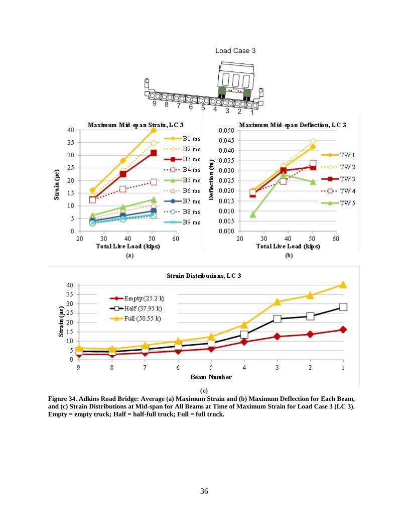
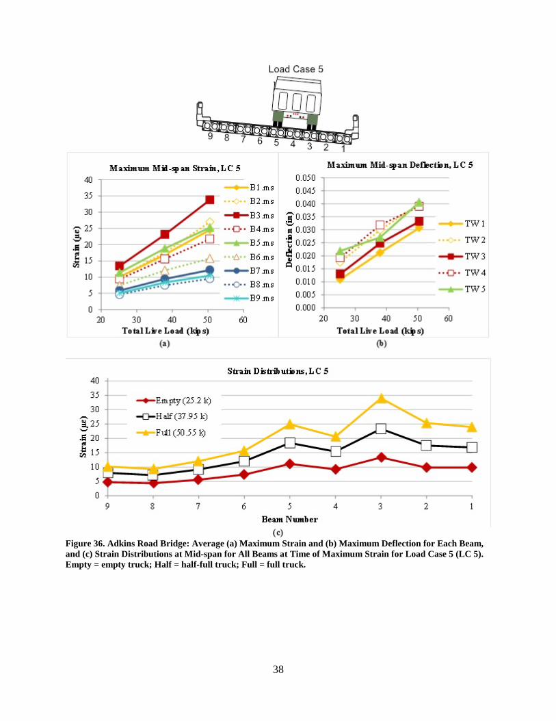
Figure 30 details a typical strain and deflection plot as a specific load truck traversed Span 3 during a single run for a particular LC. Figures 32 through 37 show the relationship between the vehicle weight and the peak strain and deflection responses in the individual members for LCs 1 through 6, respectively. The average maximum strain and deflection values displayed in Parts (a) and (b), respectively, of Figures 32 through 37 were taken from the maximum strain or deflection recorded for each individual beam during one run for a given LC and load truck combination, regardless of when the absolute maximum strain or deflection occurred during that test run. These maximum values were then averaged over all of the runs of a given LC / load truck combination. On the other hand, Part (c) in Figures 32 through 37 shows the value of strain for each specific beam at the point in time when the global maximum strain among all nine beams was recorded during a given test run and then averaged for all test runs for a given LC / load truck combination. This comparison shows the relative strain distribution among the beams, as discussed later.

(a) (b)

-0.0050.0000.0050.0100.0150.0200.0250.0300.0350.0400.045

0 10 20 30

Def

lect

ion

(in)

Time (s)

Deflection at Mid-span, LC 1, Full.2

TW 1TW 2TW 3TW 4TW 5SP 9

-0.0050.0000.0050.0100.0150.0200.0250.0300.0350.0400.045

0 10 20 30

Def

lect

ion

(in)

Time (s)

Deflection at Mid-span, LC 3, Full.4

TW1TW2TW3TW4

34

Figure 32. Adkins Road Bridge: Average (a) Maximum Strain and (b) Maximum Deflection for Each Beam, and (c) Strain Distributions at Mid-span for All Beams at Time of Maximum Strain for Load Case 1 (LC 1). Empty = empty truck; Half = half-full truck; Full = full truck.

35


(a) (b)

(c)

36


37


38


39


40

The largest average maximum strain determined for the entire testing was 40 µε, which was for Beam 1 in LC 3 using the full truck. If one were to assume a design compressive strength of 4 ksi and a unit weight of concrete of 0.145 kcf in Eq. 5.4.2.4-1 of AASHTO LRFD Bridge Design Specifications (AASHTO, 2012) for calculating the concrete’s elastic modulus

E = 33,000wc1.5� f 'c [Eq. 1]

where E = modulus of elasticity, in ksi wc = unit weight of concrete, in kip/ft3 f ‘c = compressive strength of concrete, in ksi then this level of strain would equate to 0.15 ksi of tension in the bottom of the beam attributable to live load. If simple supports were assumed, a girder distribution factor that was slightly greater than the AASHTO-calculated factor (as discussed later), and a larger moment of inertia for the exterior beam compared to an interior beam (also discussed later), the theoretical stress attributable to the live load of the full truck would have been 0.26 ksi. One reason for the discrepancy between this theoretical value and the experimental result is that there was probably some rotational stiffness inherent in the bearings supporting the ends of Beam 1, resulting in the beam being stiffer than if the member was truly simply supported, as assumed. Nevertheless, if one were to take into account the calculated prestress losses for 26 3/8-in- diameter Grade 250 stress-relieved strands, along with the dead load of the beam and the live load stresses as measured in the field, the bottom of Beam 1 was still in compression, far from any concerns about cracking. The same was true for the interior beams that had smaller strains attributable to the live load but also smaller section moduli.

The calculated compressive force in Beam 1 was consistent with the strain versus load graphs in Figures 32 through 37, where the strains measured at mid-span increased fairly linearly up to the weight of the full truck. These linear results show that the structure remained within its linear elastic limit up to 25 tons during the load test, which was about 18 tons less than the inventory rating for a single-unit vehicle on this particular bridge, as listed in the 2011 inspection report.

The exceptions to this linearity in load-strain behavior were Beam 5 in LC 2, shown in Figure 33(a); Beam 3 in LC 6 and, to a lesser extent, Beam 6 in LC 2, shown in Figure 33(a); and Beam 2 in LC 4, shown in Figure 35(a). In these cases, the rate of increase in strain between the half truck and the full truck was greater than the increase going from the empty truck to the half truck, on a strain per unit load basis. Interestingly, the instances with Beam 5 and Beam 3 occurred with a wheel line adjacent to the beam in question, as opposed to being directly on top of Beam 6 and Beam 2. These increases could indicate that the beams were getting closer to their elastic limits. However, the deviation from the linear strain increase for Beam 5 and Beam 3 was only about 5 µε, which is negligible. Further, the relatively small rate of change suggests that there was still some room to increase the load if desired, as suggested by the relatively low ratio of the experimental-to-design stress.

41

There were some cases where the rate of strain increase was lower as the amount of load increased. These latter instances, however, occurred in beams that were adjacent to the more directly loaded beams. So, these anomalies may be attributed to minor changes in load distribution as the loading increased. Interestingly, Beam 4 appeared to indicate fairly consistent strain linearity as the load increased. This observation suggests that the broken strands at the quarter-point of that beam did not adversely affect the structural performance at mid-span. Further, Span 3 was 38.75 ft long, and the development length for the prestressing strands was estimated to be about 6 ft. Thus, the strands in Beam 4 were likely fully developed at mid-span despite the ruptures at the quarter-points. Therefore, the larger strains at mid-span of Beam 4 were probably not due to a lower flexural capacity compared to the adjacent members.

Another way to view the strain results for Figures 32 through 37 is to compare beams that had similar loading conditions, albeit in different LCs. The plots in Figure 38, which compare the average maximum strains for Beam 4 to those of Beams 5 and 6 under select LCs in Subplots (a), (b), and (c), respectively, may be taken as examples. The difference between Subplots (a) and (c) is that Subplot (a) shows data when a wheel line was directly on the centerline of the indicated beam whereas Subplot (c) has the two wheel lines straddling the beam. In each comparison, the measured strains were virtually identical, where the largest difference was about 5 µε when the left wheel line was on top of Beam 4 versus Beam 6, again indicating that the broken strands in Beam 4 did not have a large impact on the strength of the beam.

For another comparison, the graphs in Figure 39 may be considered, which pair the results for a beam in the southbound lane with the average maximum strain recorded for a beam in the northbound lane that was symmetric to the bridge centerline and subjected to a similar load pattern as shown in Figure 39(a), LCs 3 and 1, respectively, and Figure 39(b), LCs 4 and 2, respectively. The beams in Figure 39 are paired together in the figure legend according to their symmetric location; plots for the beams in the southbound lane are solid lines, whereas plots for the beams in the northbound lane are dotted lines. In other words, Beam 1 (solid line) is paired with Beam 9 (dotted line), Beam 2 (solid line) is paired with Beam 8 (dotted line), etc. Figure 40 is more of a reconfiguration of the results for LC 6 in Figure 37(a), but again beams that were symmetric to the bridge centerline are coupled together. For the most part, all three scenarios in Figures 38 through 40 demonstrate that the peak strains in the beams in the southbound lane were generally slightly greater than those in the northbound lane. The southbound lane is the lane on the lower end of the superelevation. Thus, the southbound lane was likely the side of the bridge where snow would pile up during snow removal and certainly the side subjected to more chloride during snow melts and rain runoff. Thus, the beams in the southbound lane could conceivably have had a greater degree of deterioration and, thus, this could have been the reason that lane exhibited larger strains during the load test.

With that said, one fact that should be highlighted is that the differences in strain between the two travel lanes were minute. For added emphasis, as mentioned previously, despite the maximum live load strain seen during all of the testing, the net stress in the bottom of the prestressed concrete voided slabs was still compressive. However, the maximum test load was only 68% of the inventory rating load for an HS20 vehicle, according to the 2011 inspection report. In addition, the testing did not include dynamic effects because of situational limitations.

42

However, the information gained from the load test could be used to model or estimate the safe load capacity of the structure and compare that result with the previous rating.

The results for the deflection data in Figures 32 through 37 suggested responses similar to

those observed with the strain data except for the fact that the deflectometer for Beam 5 tended to measure a much smaller rate of deflection increase as the amount of live load increased. There is even one case where the average maximum deflection in Beam 5 for LC 3, shown in Figure 34(b), was lower under the full truck load compared to the deflection caused by the half truck load. This observation does not agree with the strain results shown in Figure 34(a), where the measured increase in strain resulting from the full truck load was proportional to the strain increase because of the half truck load.

Figure 38. Adkins Road Bridge: Given Similar Loading Conditions, Comparison of Strain in Beam 4 to Strain in (a) Beam 5 With Both Beams Directly Loaded, (b) Beam 6, and (c) Beam 5 With Each Beam Straddled by Wheel Loads. B = beam; LC = load case.

43

Figure 39. Adkins Road Bridge: Comparison of Strains in Beams Symmetric to Bridge Centerline for (a) Load Cases 1 and 3 (LC 1 and LC 3), and (b) Load Cases 2 and 4 (LC 2 and LC 4). B = beam; LC = load case.

Figure 40. Adkins Road Bridge: Comparison of Strains in Beams Symmetric to Bridge Centerline for Load Case 6 (LC 6). B = beam.

Further investigation of the deflection data for Beam 5 showed that the standard deviation within the datasets for both the half and full trucks in the LC 3 orientation was much greater for Beam 5 compared to the other four beams. In addition, the recorded deflection for Beam 5 during the second run for the half truck appeared to increase much faster compared to other beams that were directly underneath the wheel lines, particularly when the truck had just started

44

to cross the instrumented span. Thus, the data from this particular run for this particular beam may not be valid. The reason for the variation in results may have been the poor attachment of the deflectometer to the bottom of the beam, or perhaps the device was not sufficiently anchored to the bottom of the riverbed.

Regardless, the experimental deflection values were rather small compared to what was expected. The largest average maximum deflection was 0.047 in Beam 4, observed during LC 6 with a full truck on the bridge. However, the passenger-side wheel line was directly over Beam 4 in this particular LC. As with the other LCs, the beam or beams underneath this wheel line typically had the largest response of all the beams. Thus, the fact that Beam 4 had the greatest deflection is not necessarily a cause for alarm despite the fact that this member contained broken strands. If one were to assume that the beam was a simply supported uncracked member and that the percentage of load from the full truck directly applied to that beam was 22% (which will be explained further), then the theoretical maximum deflection because of the full truck load would have been 0.183 in, or almost 3 times the measured deflection. The conclusion from this observation is that Beam 4, along with the other beams, appeared to be much stiffer than suggested by traditional analysis. A correlating conclusion could be that the beams were not truly simply supported and that some rotational restraint was provided at the ends of the beams, as discussed later. Load Distribution Factors, g

Regarding the load distribution graphs shown in Figures 32 through 37, if the load were evenly spread out across all the beams in a bridge, the amount of strain in each beam would be identical. However, if the weight of a truck is borne solely by the beams directly underneath the truck’s wheels, then a more localized distribution of the load would be indicated by a sizable change in the strain in those beams relative to the other members. Although all of the LCs during this test had distribution results that were somewhere between these two outcomes, LCs 1 and 2 were closer to the former scenario, where Beams 5 through 9 had a relatively similar amount of strain (at the time of maximum strain) when the truck was located on the elevated half of the bridge.

On the other hand, the remaining LCs do show a little bit of a spike in the load distribution graphs. This spike was most evident in LC 6, when one of the wheel paths of the load truck was directly over Beam 4. Given that similar, albeit less prominent, changes in strain levels occurred in LCs 3 through 5, where a wheel path was over or adjacent to Beam 4, the data indicate that the longitudinal joints on either side of Beam 4 were no longer intact. Although the researchers observed that there was virtually no efflorescence at these two joints, the damage to the joints may have been relatively recent such that mineral buildup did not have sufficient time to develop. Regardless, there was at least some degree of load distribution occurring in each of the six LCs, as indicated by the amount of strain in all of the beams, with the exception of those members farthest away from the load truck.

The data in Figures 32 through 37 can be condensed to a single value, known as the load distribution factor, g. This factor is the fraction of the vehicular load that is directly applied to any one beam, expressed as the ratio of the maximum strain found among all the beams divided

45

by the sum of the strains in all the beams at the time the maximum strain was recorded. The greater the value of g, the lower the amount of load being distributed to the beams adjacent to the beam that is directly underneath the wheel load.

The average distribution factors for moment for each of the six LCs are tabulated in Table 6. The largest average factor was 0.24 for LC 3, based on a total of six runs for three load trucks. In comparison, Table 4.6.2.2.2b-1 of the AASHTO LRFD Bridge Design Specifications (AASHTO, 2012) provides formulas for calculating the design live load moment distribution factors for bridges constructed of precast voided boxes with shear keys but with no cast-in-place deck overlay.

The calculated values for g are given in Table 7. There are two possible calculations

depending on whether there is sufficient transverse post-tensioning to cause the individual box sections to act as a complete unit or the post-tensioning that is provided inhibits only vertical displacement at the beam interface. In addition, the distribution factor calculation depends on whether the beam is an exterior beam or an interior member. Regardless, all of the results in Table 7 were based on the assumption that one design lane was loaded, as there was only one truck on the bridge during testing. These calculations also reflected the assumption that the curvature of the structure in the plan was relatively small (less than 12 degrees, according to Article 4.6.2.2.1 and Article 4.6.1.2.3 in the AASHTO bridge design specifications [AASHTO, 2012]). In the case of the Adkins Road Bridge, the central angle was less than 3 degrees, so the curvature of the structure was not an issue.

As the largest experimental value for g found from six LCs, 0.24 could be considered the

distribution factor for the entire bridge. However, the LC that generated the maximum distribution factor, LC 3, had a wheel line being supported by both an exterior and an interior girder. Thus, determining whether the interior beam or exterior beam was the controlling element in this load test was difficult.

Table 6. Adkins Road Bridge: Moment Load Distribution Factors Based on Strain Measurements From the Various Load Cases

Load Case

Distribution Factor Average Coefficient of Variation

1 0.17 0.02 2 0.17 0.01 3 0.24 0.03 4 0.20 0.04 5 0.18 0.04 6 0.22 0.00

Table 7. Adkins Road Bridge: Distribution Factors Calculated in Accordance With AASHTOa

Post-Tensioning Condition

g Interior Exterior

Beams act as complete unit 0.21 0.23 No vertical displacement at interface 0.26 0.28

aAASHTO, 2012.

46

Further, none of the various truck orientations included a wheel line directly over either of the exterior beams because of the curbs and parapets along the edges of the deck. Therefore, comparing the calculated g for the exterior girders with the physical load test was not possible. Nonetheless, one can consider the results in Table 6 for LC 2 and LCs 4 through 6, where only interior girders were loaded and the wheel line was directly above a single beam versus on a joint between two members. For these three cases, g ranged from 0.17 to 0.22. Given that these values were closer to 0.21 than 0.26 from Table 7, the conclusion is that the individual interior beams were acting as a single unit. For LC.4, g was 0.22; therefore, 22% of the full truck load was applied to Beam 4 in calculating the theoretical deflection for that member, as discussed later. Strains at the Quarter-spans

As mentioned previously, the BDI node used to transmit sensor information from the strain gauges at the quarter-point closest to Bent 2 was not properly configured. Thus, the case for symmetry with the other end of the beam could not be confirmed. Nevertheless, Table 8 compares the average maximum strain at the measured quarter-points in Beams 3 and 4 along with the average maximum strain at mid-span with the passenger-side wheel line directly over the respective beam. Beam 4 was the voided slab that had broken strands near the quarter-point in question; these broken strands contributed no resistance to flexural strain at that location. Thus, the strain at the bottom of Beam 4 should have been greater compared to Beam 3 at the quarter-point. However, Beam 4 had noticeably lower strains at that location relative to Beam 3. On the other hand, Table 8 also lists the average maximum strain at mid-span and quarter-span for Beam 3 during LC 6, which again was the LC where the wheel line was directly on top of Beam 4. Despite having lower average strains at mid-span relative to Beam 4 for the same truck orientation, Beam 3 had larger strains at the quarter-span. Perhaps delaminations near the broken strands in Beam 4 were not visibly apparent such that debonding along the strand-concrete interface or internal cracking in the concrete prevented stresses from transferring through the material to the strain sensor at that quarter-point for Beam 4.

Table 8. Adkins Road Bridge: Average Maximum Strain Comparison Between Mid-span

and a Quarter-Point for Beams 3 and 4, Loaded With a Full Truck Load Case

No.

Beam

Truck Strain (µε)

Mid-span Quarter-span 5 3 Empty 13 10

Half 23 14 Full 34 20

6 4 Empty 16 2 Half 28 4 Full 39 5

6 3 Empty 6 6 Half 11 8 Full 20 15

47

Another possibility is that poor consolidation of the concrete at the location, as shown in Figure 41, also affected the results. If there was improper consolidation, there may have been insufficient transfer length for the stress to be transmitted from the strands to the concrete. Figure 42 shows a second area in Beam 3 where poor consolidation was even more pronounced. However, this location was on the opposite quarter-point relative to the problem area in Beam 4 and, thus, is not relevant to the results in Table 8. Nonetheless, Figure 42 complements Figure 41 in pointing out issues that were present during beam fabrication.

Figure 41. Adkins Road Bridge: Poorly Consolidated Concrete Below Broken Strands Near Quarter-Point Closest to Bent 3 in Beam 4, Span 3

Figure 42. Adkins Road Bridge: Poorly Consolidated Concrete Near Quarter-Point Closest to Bent 2 in Beam 3, Span 3

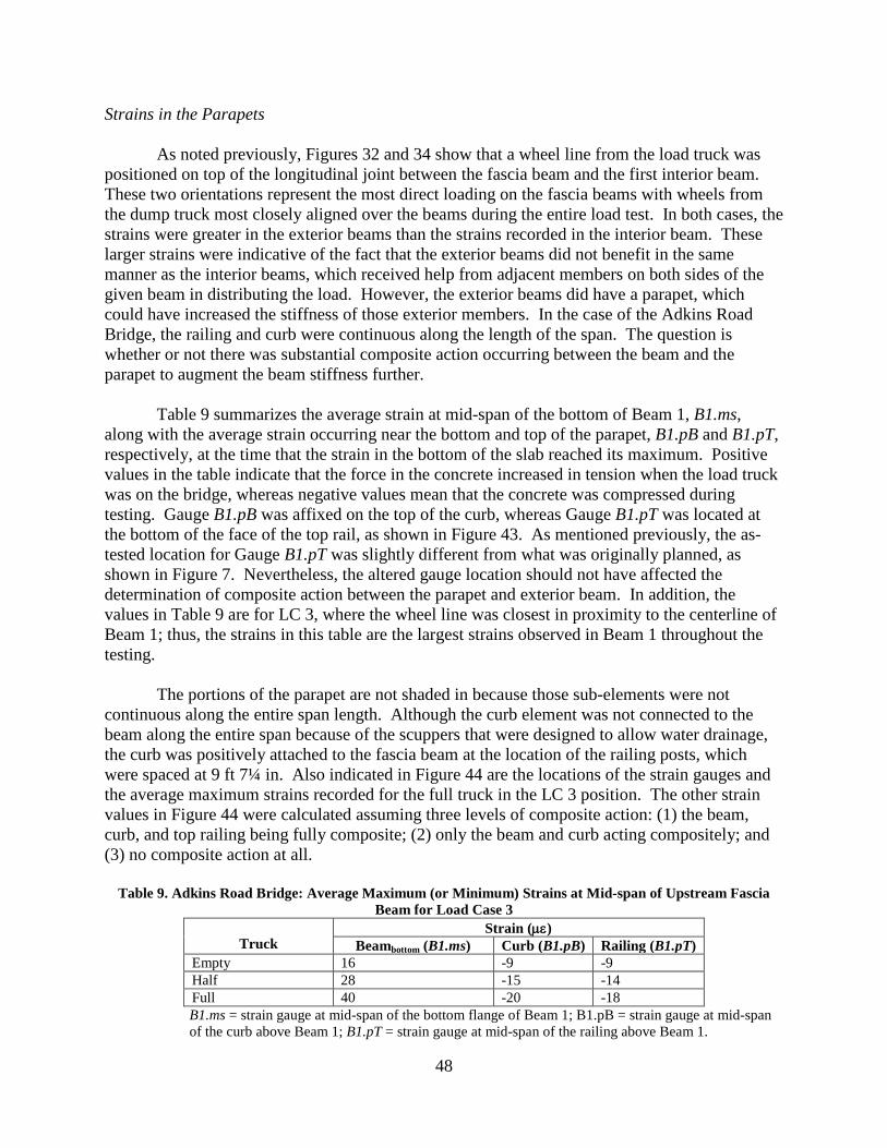
48

Strains in the Parapets As noted previously, Figures 32 and 34 show that a wheel line from the load truck was positioned on top of the longitudinal joint between the fascia beam and the first interior beam. These two orientations represent the most direct loading on the fascia beams with wheels from the dump truck most closely aligned over the beams during the entire load test. In both cases, the strains were greater in the exterior beams than the strains recorded in the interior beam. These larger strains were indicative of the fact that the exterior beams did not benefit in the same manner as the interior beams, which received help from adjacent members on both sides of the given beam in distributing the load. However, the exterior beams did have a parapet, which could have increased the stiffness of those exterior members. In the case of the Adkins Road Bridge, the railing and curb were continuous along the length of the span. The question is whether or not there was substantial composite action occurring between the beam and the parapet to augment the beam stiffness further.

Table 9 summarizes the average strain at mid-span of the bottom of Beam 1, B1.ms, along with the average strain occurring near the bottom and top of the parapet, B1.pB and B1.pT, respectively, at the time that the strain in the bottom of the slab reached its maximum. Positive values in the table indicate that the force in the concrete increased in tension when the load truck was on the bridge, whereas negative values mean that the concrete was compressed during testing. Gauge B1.pB was affixed on the top of the curb, whereas Gauge B1.pT was located at the bottom of the face of the top rail, as shown in Figure 43. As mentioned previously, the as-tested location for Gauge B1.pT was slightly different from what was originally planned, as shown in Figure 7. Nevertheless, the altered gauge location should not have affected the determination of composite action between the parapet and exterior beam. In addition, the values in Table 9 are for LC 3, where the wheel line was closest in proximity to the centerline of Beam 1; thus, the strains in this table are the largest strains observed in Beam 1 throughout the testing.

The portions of the parapet are not shaded in because those sub-elements were not

continuous along the entire span length. Although the curb element was not connected to the beam along the entire span because of the scuppers that were designed to allow water drainage, the curb was positively attached to the fascia beam at the location of the railing posts, which were spaced at 9 ft 7¼ in. Also indicated in Figure 44 are the locations of the strain gauges and the average maximum strains recorded for the full truck in the LC 3 position. The other strain values in Figure 44 were calculated assuming three levels of composite action: (1) the beam, curb, and top railing being fully composite; (2) only the beam and curb acting compositely; and (3) no composite action at all.

Table 9. Adkins Road Bridge: Average Maximum (or Minimum) Strains at Mid-span of Upstream Fascia Beam for Load Case 3

Truck

Strain (µε) Beambottom (B1.ms) Curb (B1.pB) Railing (B1.pT)

Empty 16 -9 -9 Half 28 -15 -14 Full 40 -20 -18

B1.ms = strain gauge at mid-span of the bottom flange of Beam 1; B1.pB = strain gauge at mid-span of the curb above Beam 1; B1.pT = strain gauge at mid-span of the railing above Beam 1.

49

Figure 43. Strain Gauge Locations on Parapet of Adkins Road Bridge

Figure 44. Adkins Road Bridge: Comparison of Experimentally Measured Strains Versus Calculated Values Assuming Various Degrees of Composite Action. Exp. = experimental; Comp. = composite.

In calculating the theoretical strains for the given levels of composition, the compressive strength of the concrete in the beam was assumed to be 4 ksi and the strength of the curb and railing was assumed to be 2.5 ksi. The section properties of the curb and railing were transformed to that of the beam using calculated values for the modulus of elasticity in accordance with Equation 1. Varying the assumed compressive strength, and hence the elastic modulus, did not have a major impact on the calculated strain values given in Figure 44. The moment applied to the composite portion of the structure was assumed using the weight of the

B1.pB

B1.pT

50

fully loaded truck on a simply supported structure multiplied by the girder distribution factor for LC 3 in Table 6 (i.e., 0.24).

With regard to comparing the experimentally recorded strains versus the calculated

values, there was apparently a small degree of composite action occurring between the exterior beam and the parapet components. If, in fact, the railing was behaving non-compositely in bending, the railing would at least be slightly in tension near the bottom of the element because of self-weight because the supporting beam would have deflected away from the railing as the load truck crossed the span. Instead, the load test showed that the bottom of the railing was slightly in compression. Likewise, a non-composite curb would have registered very little strain, as the strain gauge was close to the curb’s neutral axis. Yet, the measured strain was greater, albeit far less than if the curb had been fully composite with the beam. Differential Displacements Between Beams

Figure 45 shows a comparison in the typical behavior of two longitudinal joints at the mid-span of Span 3, where Joint 1 was considered to be a representative joint in poor condition whereas Joint 7 was similar to other joints deemed to be in relatively good condition based on visual observation of the underside of the bridge. Figure 45 reflects a full truck for two LCs, LC 4 and LC 2, for the two respective joints. These two LCs are the only comparable truck orientations where a wheel line from the load vehicle was adjacent to a longitudinal joint at which differential displacement was measured. Although the truck orientations themselves were symmetrical with respect to the centerline of the bridge, the two joints did not receive quite the same loads. The difference lies in the fact that Joint 1 was primarily loaded with the passenger side of the truck whereas the driver side of the vehicle was adjacent to Joint 7. Again, because of the nature of the weight distribution of the truck, Joint 1 experienced about 2% greater load than Joint 7.

Despite the slight differences in loading, the relative displacements at both joints were

extremely small, with the largest vertical differential movement being just above 0.001 in. Interestingly, the differential horizontal displacement was greater than the vertical displacement in both joints. Even so, the recorded displacements were below the precision in the LVDTs, which was 0.005 in. Nevertheless, just as a point of comparison, the two longitudinal joints had a similar degree of horizontal movement between the two beams at the given joint. On the other hand, Joint 1 had about twice as much vertical differential movement as did Joint 7. Again, however, greater emphasis should be placed on the fact that all of the measured movements between two beams were minute.

With regard solely to Joint 1, Figure 46 shows a typical comparison of the movement

between Beams 1 and 2 under two load scenarios. Figure 46(a) shows the behavior when a wheel line from the load truck was positioned directly over the joint; Figure 46(b) shows the result of having a wheel line centered on a beam adjacent to the joint. The measurements in these plots are quite small; nevertheless, the vertical differential displacement was marginally greater for LC 4.

51

Figure 45. Adkins Road Bridge: Comparison of Differential Displacements at Mid-span for Joints 1 and 7. Jt. = Joint; vert. = vertical; horz. = horizontal.

Figure 46. Adkins Road Bridge: Differential Displacements Between Beams 1 and 2 for (a) Load Case 3 (LC 3), and (b) Load Case 4 (LC 4). vert. = vertical; horz. = horizontal.

0.000

0.001

0.002

0.003

0.004

0 5 10 15 20 25

Dis

plac

emen

t(in

)

Time (s)

Differential Displacements

Jt. 1 vert.

Jt. 1 horz.

Jt. 7 vert.

Jt. 7 horz.

(a) (b)

-0.001

0.000

0.001

0.002

0.003

0.004

0 5 10 15 20 25

Disp

lace

men

t (in

)

Time (s)

Differential Displacements, Joint 1, LC 3

Q1 vert.Q1 horz.MS vert.MS horz.Q3 vert.Q3 horz.

-0.001

0.000

0.001

0.002

0.003

0.004

0 5 10 15 20 25

Disp

lace

men

t (in

)

Time (s)

Differential Displacements, Joint 1, LC 4

Q1 vert.Q1 horz.MS vert.MS horz.Q3 vert.Q3 horz.

52

Beam Rotations

As stated earlier, the intent of placing tiltmeters at both ends of Beam 4 had been to compare the rotations of the two ends near their supports. However, the data collection system was not properly configured to receive information from the tiltmeter located at the end of Beam 4 at Bent 2. Thus, no comparison could be made between the two ends of the beam. Nevertheless, the rotation at the one end of the beam appeared to be fairly small and fairly consistent for LCs 3 through 6, as shown in Table 10. Even for the most heavily loaded vehicle, the rotation of the beam end had an average maximum value of about 0.014 degrees. That peak occurred when the front axle was off the span and the center of the tandem axle was located at approximately 23.5 ft, or about 60% of the span length (0.6L). The manufacturer’s specified 0.0005 degree resolution for the tiltmeter blurs the fact that the accuracy for the device was only 0.2 degrees. Nevertheless, Figure 47 shows that the tiltmeter did indicate that the load truck was on the span, regardless of how heavily the beam was loaded. The calculated rotation for an apparent intact beam subjected to the truck loads (with the assumed factors discussed in a prior section, Load Distribution Factors, g,) was 0.07 degrees.

The voided slab structure in the Adkins Road Bridge was evidently restrained at the

supports compared to the theoretically simply supported superstructure members. If so, this restraint could provide some explanation as to why the measured deflections in the beams were so small compared to theoretical deflections for simply supported flexural members. The cause of the restraint may partly be attributed to standard anchorage details at the time the bridge was originally built whereby each of the beams was anchored to the pier support by the use of 3/4-in dowel bars cast vertically into the pier caps and then going through the beams, as shown in Figure 48.

Although the older design was not intended to be a moment connection, perhaps the

dowel bars provided some resistance to bending, thus resulting in smaller rotations and even lower strains. Current design standards call for only the fascia beams to be anchored on their external faces in order to prevent the internal beams from moving laterally.

Table 10. Adkins Road Bridge: Average Maximum Measured Rotations, in Degrees, for Beam 4 Near Bent 3

Truck

Load Case 3 4 5 6

Empty 0.006 0.006 0.006 0.007 Half 0.009 0.009 0.009 0.01 Full 0.012 0.012 0.012 0.014

53

Figure 47. Adkins Road Bridge: Typical Plots Showing Rotation of Beam 4 Near Pier 3 as a Given Load Truck Crossed Span. Empty = empty truck; Half = half-full truck; Full = full truck.

Figure 48. Anchorage Details Connecting Voided Slabs to Substructure of Adkins Road Bridge

54

CONCLUSIONS • Drainage patterns are closely related to the deterioration mechanisms of superstructures.

The Qualla Road Bridge overlay had a camber in the middle, so the drainage was

designed to flow to either side and through the scuppers over the external sides of the fascia beams. There were pop-outs on the sides of fascia beams, as shown in Figure 11, which are more likely attributable to the stagnation and flow of the salt-laden water over the exposed sides and the lower concrete cover depths.

The Adkins Road Bridge had a significant cross slope, causing the drainage to flow to the upstream side of the bridge and out through the scuppers. There was significant scaling on the exposed side of the fascia beam.

• A number of mechanisms result in accelerated deterioration of bridges. Accumulated dirt and vegetation growing at the scuppers obstructed the free drainage of

runoff. As a consequence, chloride-laden water penetrated the concrete in these locations.

Reflective longitudinal cracks formed through the asphalt riding surface, allowing chloride-laden water to drain through the joints and wet the top, sides, and bottom of the beams.

Clear concrete cover thicknesses were generally less than specified at a considerable number of locations, especially at the bottom of the slabs.

For the Qualla Road Bridge in particular, the concrete showed moderate chloride ion penetrability in permeability testing.

• The Adkins Road Bridge still retained adequate flexural strength to support service loads.

The beams in the Adkins Road Bridge were still within their elastic limit, as supported by

the generally linear strain versus load and the deflection versus load plots in Figures 32 through 37.

In agreement with the previous point, the bottoms of the voided slabs were calculated to be in compression throughout the load test. Although the maximum applied load was less than 70% of the existing inventory rating load and the testing did not include dynamic effects, results from this study could aid in reevaluating a new inventory rating.

The broken strands in Beam 4 of the Adkins Road Bridge did not appear to have a large negative impact on the beam’s flexural capacity relative to the adjacent beams when subjected to similar loading conditions.

55

The beams in the Adkins Road Bridge were much stiffer than expected, possibly as a result of rotation being restrained at the supports. In addition, the exterior girders benefitted from the stiffness provided by the barriers, which exhibited some degree of composite action with the fascia beams.

• The AASHTO-calculated girder distribution factor for interior adjacent members where

there is no vertical displacement at the interface between beams is sufficient for analyzing adjacent member structures. There were virtually no vertical or horizontal differential displacements at the two joints

that were monitored during the load test of the Adkins Road Bridge.

The girder distribution factors for various LCs were actually less than the design factor, assuming that the individual voided slabs acted as a complete unit. However, when the coefficient of variation is taken into account, assuming that the voided slabs act as one unit would be slightly non-conservative.

The longitudinal joints adjacent to Beam 4 in the Adkins Road Bridge no longer appeared to be intact because of the small amount of efflorescence forming on the bottom of this member and the two adjacent beams. Yet, there was still some degree of load distribution across these longitudinal joints.

Because of the curbs on top of the deck, determining g for an exterior beam was not possible.

• The results suggest that evaluating bridges considered for replacement with the use of NDE techniques, such as determining material and structural conditions, might delay replacement for a number of years and thus free up resources for other needed projects.

RECOMMENDATIONS 1. VDOT’s Structure and Bridge Division should revise its guidance on design, construction,

and maintenance of adjacent member prestressed structures such as voided slabs to address issues identified in this study such as failing longitudinal shear transfer mechanisms and the resultant salt-laden moisture infiltration through the sides and bottom of adjacent slabs. A list of recommended changes based on the results of this study is provided in the Appendix.

BENEFITS AND IMPLEMENTATION

Benefits

Implementation of Recommendation 1 will lead to improved service life and reduced overall maintenance costs of adjacent member structures. Further, adoption of the NDE techniques used in this study and described in the Appendix will help to identify deterioration

56

issues that are not easily visible. Addressing these issues with preventative measures such as those already in practice and those recommended in this report will also help in improving the service life of this class of structures and reducing the costs associated with their maintenance.

Implementation With regard to Recommendation 1, staff of the Virginia Transportation Research Council

will work with members of the design and bridge management teams in VDOT’s Structure and Bridge Division to modify the noted guidance in the Manual of the Structure and Bridge Division. The modifications will be complete by June 2018.

ACKNOWLEDGMENTS

The authors recognize Rick Childs, who prepared all of the powdered samples from the concrete cores extracted from the beams as one of his last duties at the Virginia Transportation Research Council before his retirement. Other personnel associated with the material analysis included Linda DeGrasse, Nick Goddeau, Evelina Khakimova, and Lewis Lloyd. Thanks also go to Robert Dunn, Brad Jones, and Gary Martin for their cooperation and coordination for the sampling and testing of the two bridges in this study.

REFERENCES American Association of State Highway and Transportation Officials. AASHTO LRFD Bridge

Design Specifications, 6th Edition. Washington, DC, 2012. ASTM International. ASTM C876: Standard Test Method for Corrosion Potentials of Uncoated

Reinforcing Steel in Concrete. West Conshohocken, PA, 2009. ASTM International. ASTM C1152: Standard Test Method for Acid-Soluble Chloride in Mortar

and Concrete. West Conshohocken, PA, 2012a. ASTM International. ASTM C1202: Standard Test Method for Electrical Indication of

Concrete's Ability to Resist Chloride Ion Penetration. West Conshohocken, PA, 2012b. Balakumaran, S. Corrosion Testing and Modeling of Chloride-Induced Corrosion Deterioration

of Concrete Bridge Decks. Ph.D. dissertation. Virginia Polytechnic Institute and State University, Blacksburg, 2012.

Virginia Department of Transportation. Manual of the Structure and Bridge Division, Vol. 2:

Design Aids and Typical Details. Richmond, 2014. Virginia Department of Transportation. Road and Bridge Specifications. Richmond, 2016.

57

APPENDIX

RECOMMENDED CHANGES TO GUIDANCE BY VDOT’S STRUCTURE AND BRIDGE DIVISION ON DESIGN, CONSTRUCTION, AND MAINTENANCE

OF ADJACENT MEMBER PRESTRESSED STRUCTURES Design and Construction 1. Improved specifications should be established for the construction of new adjacent member

beams. Drainage patterns between adjacent member beams influence the deterioration mechanism of such elements. Therefore, the tops, the sides below the shear key, and the bottoms of the voided beams should be coated with waterproofing material, such as epoxy, prior to installation. In addition, a shallow V-groove should be cast into the bottom near both edges of individual beams. Such a V-groove should prevent water that may leak through a longitudinal beam joint from traveling across the soffit and penetrating the concrete from the bottom. This groove will likely work much the same way as a drip bead does for the soffit of an overhang.

2. For prestressed concrete adjacent member structures without a cast-in-place overlay,

AASHTO’s girder distribution factors that assume the longitudinal joints prevent only relative vertical displacement should be used (AASHTO, 2012). Although assuming that adjacent prestressed concrete members act as a complete unit might be acceptable in most cases, such an assumption might be non-conservative in some cases.

Maintenance 3. During routine preventive maintenance procedures, accumulated dirt, debris, and vegetation

should be removed from the deck as well as the superstructure. This maintenance should prevent the retention of moisture that could infiltrate the concrete.

4. For existing structures with minimal prior exposure to deicing salts, the bottom and the

exposed sides of the fascia beams should be coated with waterproofing material. As stated previously, drainage patterns influence the deterioration mechanism of adjacent member superstructures. If there is any doubt about the level of the chloride exposure, concrete resistivity, half-cell potentials, and chloride contents should be determined at locations along the beams based on the drainage pattern. The edges of each of the beams should be retrofitted with a drip edge if none exists; one method is a post-installed angle anchored to the soffit.

5. For existing structures with high prior exposure to chlorides, values for concrete resistivity,

half-cell potentials, and chloride contents should be determined at locations along the beams based on the drainage pattern. Generally, this recommendation applies to older structures or those located in a region subjected to major deicing salt usage. Potential locations for determining the aforementioned values are the exterior sides of the fascia beams and near the edges of the bottom of beams that may show indications of deterioration. If the test results are acceptable, the structure should be retrofitted as though the bridge had only minor chloride exposure (see Number 4). If the test results indicate severe local corrosion, the damaged

58

beams should be replaced provided that replacement of an individual beam is cost-effective. If corrosion is severe and widespread throughout the entire superstructure, total replacement is recommended.

6. For voided beam structures with evidence of water infiltration through the longitudinal joints between adjacent beams, a robustly functioning, moisture-resistant detail should be considered for the shear key.

Inspection and Evaluation 7. Multiple forensic techniques should be considered concurrently instead of simply relying on

one method. Concrete resistivity, half-cell potentials, and chloride concentrations provide different measures of corrosion. However, these parameters provide the clearest assessment of the condition of the steel reinforcement when viewed together.

8. Infrared thermography holds promise as an NDE technique, but it needs further refinement to be practical for field applications. Coatings and other markings on the surface can interfere with images captured using an IR camera using static/passive methods. Further, work underneath the bridge deck often requires “active” infrared thermography, where special equipment is used to induce heat gradients in order to obtain heat signatures from the concrete beams that are different from that of the ambient air. Time-lapse thermography, an improvement over conventional infrared thermography that involves nearly continuous recording of the surface temperature of the target area, should be considered.

9. Bridge managers should use the data presented in this report to generate models that include the prescribed legal load and dynamic effects for future rating analysis of similar deteriorated adjacent prestressed voided beam structures. The modeling should assume some rotational restraint at the supports.

Documents

Forensic Investigation of Two Voided Slab Bridges in the … · Forensic Investigation of Two Voided Slab Bridges in the Virginia Department of Transportation’s Richmond District