Embed Size (px)
Citation preview
Foreign Firms and Host-Country Productivity:
Does the Mode of Entry Matter?∗
Ragnhild Balsvik† Stefanie A. Haller‡
October 2009
Abstract
Foreign direct investment is considered an important source of knowledge spillovers.
We argue that the effects of foreign presence on host country productivity may differ
depending on the mode of foreign entry. Using a long panel from the Norwegian Man-
ufacturing Census, we find that greenfield entry both in the same industry and in the
same labour market region has a negative impact on the productivity of domestic plants,
while entry via acquisition affects the productivity of domestic plants in the same industry
positively. The positive effect from acquisitions is consistent with knowledge spillovers as
these plants have pre-established linkages within the industry. The negative effects from
greenfield entry can be attributed to increased competition both in the product market
and for qualified employees in a tight labour market. This may help to explain the am-
biguity of results in the empirical literature that relates overall foreign presence to host
country productivity.
Keywords: mode of foreign entry, productivity, competition, spillovers
JEL Classification: D24, L1, F21∗We are grateful for valuable comments from and discussions with Carlo Altomonte, Davide Castellani,
Chiara Criscuolo, Holger Gorg, Lisa Lynch, Jarle Møen, Øivind Anti Nilsen, Kjell Gunnar Salvanes, Fabio Schi-antarelli and seminar participants at the Nordic International Trade Seminars in Helsinki, 2005. All remainingerrors are our own.
†Norwegian School of Economics and Business Administration, Helleveien 30, 5045 Bergen, Norway; email:[email protected]
‡Economic and Social Research Institute, Whitaker Square, Sir John Rogerson’s Quay, Dublin 2, Ireland;email: [email protected]
1
1 Introduction
The increase in foreign-direct investment (FDI) over the past 25 years has been one of the main
features of globalisation. Foreign direct investment stock as a share of world gross domestic
product increased from 5% in 1982 to nearly 26% in 2006. At least since the mid-1990s cross-
border mergers and acquisitions (M&As) have become the most important component of FDI;
in 2006 cross-border M&As accounted for over 70% of worldwide FDI outflows (UNCTAD 2007,
p.9). Caves (1974) was first to note that foreign direct investment creates a potential both for
the diffusion of advanced technological and organisational knowledge to host country firms as
well as for increased competition in host countries. Both effects have the potential to raise
the productivity of domestic plants; however, Gorg and Greenaway (2004) in their survey of
the literature find the evidence on the existence and sign of spillovers from foreign-owned to
local firms in narrowly defined industries to be inconclusive.1 A possible explanation for this
ambiguity of results is that FDI is not a homogenous phenomenon. The potential for spillovers
to arise depends on both the capacity of domestic plants to absorb them as well as on the
potential of the foreign multinationals to generate spillovers. Previous studies asking whether
heterogeneity in FDI matters for spillovers have for example split FDI according to the degree
of foreign ownership (Blomstrom and Sjoholm, 1999; Dimelis and Louri, 2001; Smarzynska
Javorcik and Spatareanu, 2008), the motivation for FDI (Driffield and Love, 2006), and different
characteristics of the foreign affiliates (Castellani and Zanfei, 2006).
We investigate whether the mode of entry of foreign-owned firms matters for productivity
spillovers to domestic firms. For foreign investors it is an important strategic choice whether
to enter a new market via greenfield investment or through acquisition of assets in the host
country. This choice also affects market structure in the host country differently: greenfield
entry adds production capacity while acquisition entry only changes ownership and control
over existing assets. In addition, given the different degrees to which greenfield and acquisition
ventures are embedded in the local economy around the time of entry, the two entry modes
1Among the more recent studies, Aitken and Harrison (1999) find a negative effect for Venezuela, as doKonings (2001) for Poland, Bulgaria and Romania, and Djankov and Hoeckman (2000) for the Czech republic.On the other hand Haskel et al. (2007) and Keller and Yeaple (2009) find evidence of positive spillovers for theUK and the US, respectively.
2

may have different effects on the domestic firms in the same sector or region. As noted above a
large share of FDI takes the form of cross-border mergers and acquisitions and most countries
receive FDI through both modes of entry. Therefore, combining these two modes of entry into
a single measure of foreign presence in the sector, as is common in the literature, may give rise
to ambiguous results. We estimate production functions for the domestic plants augmented
by terms that capture foreign presence in the same sector and in the same region in order to
compare our results to the existing literature. We then go one step further and split this measure
of overall foreign presence into three terms, two separate terms for the new foreign entrants
differentiated by the mode of entry and another term for the existing foreign-owned firms. By
doing this we can explicitly account for the effects of foreign entry through acquisitions and
greenfield investment. In addition, we can investigate whether the extent of spillovers from
recent foreign entrants and previously established foreign-owned firms are different.
We use a large panel based on 24 years of the full census of Norwegian manufacturing plants
for the period 1978-2001. In addition, we have plant-level information on foreign ownership.
As the census captures all plants in Norwegian manufacturing, our results are not affected by
the sampling issues that most other work in this area is burdened with. The census-nature of
the data allows us to identify foreign entry with a high degree of precision. The employment
share in foreign-owned firms in Norwegian manufacturing increased from about 6.5% in 1978
to 25% in 2001. In contrast to many other developed economies Norway has not introduced
specific incentive schemes in order to attract foreign direct investment.2 Over the long sample
period Norway has seen sufficient episodes of greenfield investment and foreign acquisitions to
make it an ideal case for studying the effects of the two modes of entry on the productivity of
domestic plants in the same industry.
We estimate augmented production functions for domestic plants where output is regressed
on inputs, measures of foreign presence and the mode of foreign entry at both the industry and
2In 1994 an organisation called ‘Invest in Norway’ was set up as a separate office of the existing ‘NorwegianIndustrial and Regional Development Fund’ (SND). The aim of SND (replaced by Innovation Norway in 2004) isto stimulate business development in all parts of Norway. In line with this ‘Invest in Norway’ was to promote theestablishment of foreign firms in Norway, but it had no separate subsidy or incentive schemes for this purpose.The office worked mainly towards marketing Norway as a country to invest in and provided information tointerested investors. ‘Invest in Norway’ was closed down by the end of the 1990s (see SND’s annual reports1993-1999).
3
regional level, as well as control variables for the intensity of competition. Our results suggest
that a change in foreign presence measured as the change in the share of overall employment in
foreign-owned plants relative to total employment in a sector, has a small positive effect on the
productivity of domestic firms. When we specifically account for the change in foreign presence
in the same industry due to both greenfield entry and foreign acquisitions, we find opposite
effects of the two modes of entry. The impact of greenfield entry on domestic productivity is
negative; a 10 percentage point increase in greenfield entry last year implies a 1.9% reduction in
total factor productivity (TFP) of the domestic firms in the same sector and a 3.8% reduction
in productivity in the same labour market region. In contrast, a 10 percentage point increase
in the rate of acquisitions raises the TFP of the domestic plants in that sector by 0.8%. Our
finding of opposite effects of greenfield and acquisition entry apply to majority-owned foreign
entry. They are robust to concerns regarding selection, measurement and endogeneity. We
argue that the positive effect of foreign acquisitions on the productivity of domestic plants is
consistent with spillovers from foreign-owned plants through knowledge diffusion and positive
competition effects.The negative effect of greenfield foreign entry seems to be the result of a
market stealing effect in the product market in combination with competition for key employees
in a relatively tight labour market.
The remainder of this paper is structured as follows. In Section 2 we lay out the theoretical
and empirical background and derive conjectures about the implications of greenfield and ac-
quisition entry. In Section 3 we discuss our strategy for estimating the impact from greenfield
entry and entry by acquisition on the productivity of domestic firms. In Section 4 we describe
the data sources and give an overview of the development of foreign ownership and foreign entry
in Norwegian manufacturing. We present our estimation results and examine their robustness
to a number of different specifications in Section 5. Section 6 provides a discussion of our
results; and Section 7 briefly concludes.
2 Mode of entry and implications for host country firms
The implications of firm entry for incumbent firms, their performance and market structure
have long attracted the interest of researchers, see Geroski (1995), Siegfried and Evans (1995)
4

and Caves (1998) for surveys. This literature has not distinguished between foreign and do-
mestic entry, and relates primarily to domestic entry. In general the findings show that most
entrants are small, have a low chance of survival, and make only small contributions to industry
productivity growth, but the entry-exit process is important for longer term industry-level pro-
ductivity gains. A substantial literature has established that foreign entrants are different: they
are larger, more technology intensive and more productive than their host-county competitors
(e.g. Barba Navaretti and Venables, 2004).
Caves (1974) postulated that foreign direct investment may affect host country firms in two
ways. First, by endowing their subsidiaries with skilled entrepreneurship and/or productive
knowledge, foreign multinationals may generate spillovers to host country firms. Second, the
presence of efficient foreign subsidiaries may also increase competition in the host country. The
effects from foreign presence are likely to be felt strongest by host country competitors in the
first few years after entry. Moreover, there are several indications to suggest that these effects
differ depending on whether the foreign subsidiary was established through greenfield entry or
via acquisition of an existing plant. This applies to both the potential for knowledge diffusion
as well as the potential for increased competitive pressure. We discuss the implications for each
channel in turn.
Both types of foreign entry are likely to create potential for knowledge diffusion by enhancing
the existing knowledge stock in the host country with superior technology or organisational
skills from their headquarters abroad. In the theoretical literature on the choice between
greenfield entry and entry via acquisition it is always the most efficient firms that choose
the greenfield route (e.g. Mattoo et al. 2004, Nocke and Yeaple 2007, Norback and Persson
2008, Haller 2009). Broadly speaking, this is because they do not have to share the profits
with a local partner as greenfield investors. Javorcik and Saggi (forthc.) provide evidence
for Eastern European countries showing that greenfield entrants are more productive that
acquisition entrants. Evidence presented in Balsvik and Haller (forthc.) also suggests that
foreign greenfield entrants have higher productivity than acquisition entrants in Norwegian
manufacturing. If this is generally the case, the potential for knowledge diffusion may be larger
from greenfield entrants than from foreign acquisitions. Yet the efficient foreign entrants will
5

also have the largest incentives to protect their intellectual property, therefore actual knowledge
diffusion from these plants to competitors may be small.
A growing literature on the ownership advantages of foreign-owned firms finds that produc-
tivity in the acquired local plants increases following foreign acquisitions, thereby providing
indirect evidence that headquarters of multinationals transfer knowledge to their newly ac-
quired affiliates.3 As plants that are acquired by foreign owners operate in the local economy
already before the change in ownership, the potential for spillovers to other domestic plants
may be greater from them than from greenfield entrants. These firms will have established
linkages with the host country that the greenfield entrants have yet to build. Moreover, labour
turnover associated with the change in ownership may act as a channel for knowledge transfer
to domestic plants. If knowledge diffusion takes time to materialise, this type of spillover may
also be more likely from foreign-owned firms that have been in the market for some time. Sem-
benelli and Siotis (2008), in their analysis of the impact of FDI on markups of manufacturing
firms in Spain, find weak evidence that foreign presence dampens margins in the short run,
but also a longer-term compensating positive effect in R&D intensive industries which they
interpret as evidence of knowledge diffusion.
Regarding the competition channel there could be different forces at play: First, if entry
by new and efficient firms forces incumbents to reduce x-inefficiencies or to adopt new tech-
nologies faster than they otherwise would, average productivity in the host country industry
may increase.4 To the extent that technology and knowledge transfer is highest in the initial
years of the investment, we do not expect well-established foreign-owned firms to exert strong
positive or negative pro-competitive effects.
Second, greenfield and acquisition entry will affect competitive pressure differently due to
the way they affect market structure. While the theoretical literature on the choice between
greenfield and acquisition entry cited above emphasises market structure or rather market power
considerations as an important motive, these models are largely silent on the implications of
the mode of foreign entry for the host country firms. As noted in UNCTAD (2000, p.145), an
3Examples are McGuckin and Nguyen (1995) for the US, Harris and Robinson (2002) and Criscuolo andMartin (2009) for the UK.
4Aghion et al. (2009) demonstrate that foreign greenfield entry in the UK increases the incentives of firmsto innovate in order to survive the increased competition.
6
important difference between the two entry modes, is that greenfield entry increases production
capacity while entry via acquisition leaves production capacity unchanged at least in the short
run. The increase in production capacity following greenfield entry can lead to increased com-
petition, and, thereby, to reduced domestic market shares as argued in Aitken and Harrison
(1999). A reduction in output prices is another conceivable outcome. In contrast, unless a
foreign acquisition ends collusive behaviour in the industry, competition in the industry will
not be affected in short run. If the acquired plant undergoes substantial restructuring as a
result of the acquisition, pro-competitive effects will take longer to materialise.
In addition to increasing competition in output markets, new foreign entrants may also
increase competition in input markets. While capital goods and material inputs can be sourced
from abroad without too much difficulty, multinationals typically hire a substantial share of
their labour force locally. Given the higher wages they pay, they are likely to attract key
employees from domestic competitors. This may have a detrimental effect on the productivity
of domestic plants if they must use resources to replace these employees. This effect should be
stronger from greenfield entrants as the increase in employment in these plants in Norway is
much higher than that in plants acquired by foreign owners (Balsvik and Haller, forthc.).
3 Empirical specification
In order to examine the impact of different modes of foreign entry on the productivity of
domestic firms, we start with an augmented production function of the following form
ln Yit = βK ln Kit + βM ln Mit + βH ln Hit (1)
+T∑
k=0
βk1FPI,t−k +
T∑k=0
βk2FPR,t−k + γZit + υi + εit.
This type of equation is commonly used to investigate whether FDI generates intra-industry
spillovers (e.g. Castellani and Zanfei 2006, Haskel et al. 2007). In equation (1) ln Y , ln K,
ln M , and ln H are the natural logs of output, capital, hours and materials in plant i, year t.
For the construction of all variables, see the variable definitions in the Appendix. Z includes a
set of competition variables and υi is an unobserved plant-specific effect.
7
Given that we are controlling for input use, FPI,t−k measures the impact of foreign presence
on the productivity of domestic plants. In the previous spillover literature this is the variable of
main interest. In the case of intra-industry spillovers, FPI,t−k captures overall foreign presence
at the industry level. A positive coefficient is consistent with spillovers from foreign firms to
domestic firms in the same industry. We calculate FPI,t−k at the 5-digit ISIC level and measure
it as the share of employment in foreign-owned plants in total industry employment. We have
140 5-digit sectors in our estimations.5 Similarly FPR,t−k captures spillovers from overall foreign
presence at the region level. We calculate FPR,t−k at the labour market region level as identified
by Statistics Norway on the basis of commuting patterns (Bhuller, 2009); there are 46 labour
market regions in Norway. As the effects from foreign presence may take time to materialise,
we include 2 lags of foreign presence in our estimations.6
We use a set of variables similar to those first proposed by Nickell (1996) to control for
competition. These include industry concentration (CR5It), market share (MSit), and profit
margins (PMit). As our concentration measure we use the sum of market shares of the five
largest plants defined at the 5-digit industry level. Technological differences across industries
imply very different requirements in terms of size and scale for firms to be able to operate in their
respective environments, see Sutton (1996). High market shares, therefore, need not indicate
a lack of competition. However, as argued by Nickell (1996), changes in market structure over
time are still going to be reasonably good measures of changes in competition. The profit
margin measure is thought to capture possible rents that may be available to shareholders and
workers in the form of higher pay and lower effort. The expected signs on the concentration
measure, market share and profit margin are negative: higher profit margins allow scope for
lower effort and thus lower productivity, and higher market shares or concentration ratios are
associated with lower effort and productivity levels. As higher productivity would raise both
profit margins and market shares, these variables are potentially endogenous. We follow Haskel
et al. (2007) and address this problem by lagging both measures. We use two-period lags
and note that endogeneity would give rise to an upward bias in the estimated coefficients. We
5The mean number of plants in a 5-digit sector is 40 with a standard deviation of 60; the median number ofplants is 17.
6We also tested for longer lag lengths, but more than two lags were never significant.
8

also tried different control variables for import intensity and a control for the rate of turnover
of plants in an industry. However, these variables were never significant. Information for
import competition is only available at the 2- to 3-digit industry level, thus, our industry-year
interaction dummies described below will capture unobserved variation at this level.
It is conceivable that foreign entry is directed mainly at fast growing industries: to control
for this possibility at a more disaggregate level we include changes in 5-digit industry output and
industry employment excluding each plant’s own change in output ∆(YIt−Yit) and employment
∆(LIt−Lit). Taken together these two control variables will capture changes in average labour
productivity in the industry, hence we expect the sign on ∆(YIt − Yit) to be positive and the
sign on ∆(LIt − Lit) to be negative.
The productivity of a plant is likely to be affected by unobserved variables. We eliminate
unobserved plant-specific effects by time-differencing equation (1). Taking first-differences also
eliminates the effects from any unobserved time invariant industry or regional variables. In
our first-differenced equation we add year dummies to take account of common shocks that
may be correlated with foreign presence across all industries. By including NUTS2 region and
3-digit industry dummies, we account for both region- and industry-specific linear time trends
in the levels of the dependent variable. In addition, we add a set of 2-digit industry-year
interaction terms to account for possible correlations between foreign presence and industry-
specific shocks.7 Including these dummies further implies that our results rely on differences in
plant productivity and foreign presence or foreign entry from their year, region and industry
means rather than on differences in plant productivity across sectors or years. On the basis of
the above considerations, we estimate the following equation on the sample of plants that are
Norwegian-owned throughout their presence in our panel.
∆ ln Yit = αK∆ ln Kit + αM∆ ln Mit + αH∆ ln Hit +2∑
k=0
βk1∆FPI,t−k +
2∑k=0
βk2∆FPR,t−k (2)
+ γ1∆MSi,t−2 + γ2∆PMi,t−2 + γ3∆CR5I,t + γ4∆(YIt − Yit) + γ5∆(LIt − Lit)
+ υt + υR + υI + υIt + ξit.
7There are 5 NUTS2 regions in Norway, and 28 3-digit industries and 9 2-digit industries in our data.
9
In line with the previous spillover literature, we first estimate equation (2) taking ∆FPIt
and ∆FPRt to be the first-difference of overall foreign presence at the industry and at the
labour market region level, respectively. In what follows we use ∆FPIt for illustration, but the
decomposition applies similarly to foreign presence at the labour market region level (∆FPRt).
∆FPIt represents the change, from t− 1 to t, in overall foreign presence in the industry, and is
given as
∆FPIt =
∑i∈FOIt
(Empl)it
(Total empl)It
−
∑i∈FOI,t−1
(Empl)i,t−1
(Total empl)I,t−1
. (3)
In equation (3) FOIt is the set of foreign-owned plants in industry I at time t. A change in
foreign presence can come about through greenfield entry of foreign plants, foreign acquisitions,
employment expansion or contraction in existing foreign-owned firms, and also by foreign-
owned firms divesting or closing down.8 If recent foreign entrants have a different effect on the
productivity of domestic firms than long established foreign-owned firms, using a measure of
overall foreign presence in the regression may generate ambiguous results. The same argument
applies if different modes of entry have different effects on domestic productivity.
In our second specification we split ∆FPIt into three parts in order to isolate the effect of
some important sources of change in overall foreign presence. As our decomposition focuses
on greenfield and acquisition entry, we group the remaining possible changes from pre-existing
foreign presence into one term. The set of foreign-owned firms FOIt at time t can then be split
into the sets of greenfield entrants (GEIt), acquisition entrants (AEIt), and the set of remaining
foreign-owned plants that have been present in the sector for at least one year (FO1It), hence
FOIt = GEIt ∪ AEIt ∪ FO1It. Using these definitions of the different groups of foreign plants
in year t, we can rewrite equation (3) in the following way
∆FPIt =
∑i∈GEIt
(Empl)it
(Total empl)It
+
∑i∈AEIt
(Empl)it
(Total empl)It
+
∑i∈FO1It
(Empl)it
(Total empl)It
−
∑i∈FOI,t−1
(Empl)i,t−1
(Total empl)I,t−1
≡ GIt + AIt + ∆FIt. (4)
8Aghion et al. (2004) use the first difference of foreign presence to represent foreign entry in their study ofthe impact of entry on productivity growth in the UK, although a change in foreign presence need not only becaused by new entry of foreign firms.
10

The first term GIt in equation (4) represents the change in foreign presence between t− 1 and
t accounted for by greenfield entry. We measure this as the sum of employment in those plants
in industry I that are greenfield entrants in year t expressed as a share of total employment in
the industry that year. Similarly, AIt represents the change in foreign presence due to foreign
acquisitions in industry I between t− 1 and t. GIt and AIt represent the flow of new FDI into
the sector differentiated by the mode of entry. The last term ∆FIt equals the two terms in
brackets, and represents the remaining change in foreign presence between t − 1 and t. ∆FIt
captures employment expansion or contraction of existing foreign-owned firms relative to total
industry employment, and also withdrawal of foreign firms through divestures or plant closures.
4 Data
Our main data source is the annual census of all Norwegian manufacturing plants collected by
Statistics Norway. The Norwegian Manufacturing Statistics are collected at the plant level,
where the plant is defined as a functional unit at a single physical location, engaged mainly in
activities within a specific activity group. The plant-level variables include detailed information
on production, input use, investment, location, and industry classification (ISIC Rev. 2).
We drop plants with less than 8 employees throughout their lives and observations of plants
not in ordinary production (service units or plants under construction).9 The resulting sample
contains 150,000 observations from 10,400 plants for the period 1978-2001, with an average
plant size of 43 employees. The sample covers more than 90% of total manufacturing output
and employment.
Information about foreign ownership is recorded directly in the Manufacturing Statistics
before 1990. Plants are classified into three ownership classes; plants that are part of firms
where less than 20%, 20-50%, or more than 50% of equity is directly foreign owned. From
1991 onwards we have information on foreign ownership from the SIFON-register, which is
an annual record of foreign ownership of equity in Norwegian firms. The SIFON-register also
9In addition, we drop plants that in the Norwegian Manufacturing Statistics are classified as ‘small’ (definedas having less than 5 or 10 employees) throughout their life. The information for these plants comes mainlyfrom administrative registers and is therefore less extensive than for large plants. In particular, there is noinvestment information, which means that we are unable to construct capital measures for this group of plants.
11
records indirect foreign ownership.10 As the indirectly foreign-owned plants are more similar
to the directly foreign-owned plants than to the domestic plants in terms of mean size and
productivity, we prefer to include indirect foreign ownership into the group of foreign-owned
plants. Thus, we classify plants as foreign owned when either direct or indirect foreign ownership
of equity is above the 50% threshold.
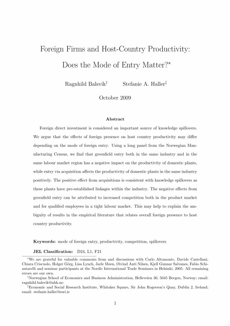
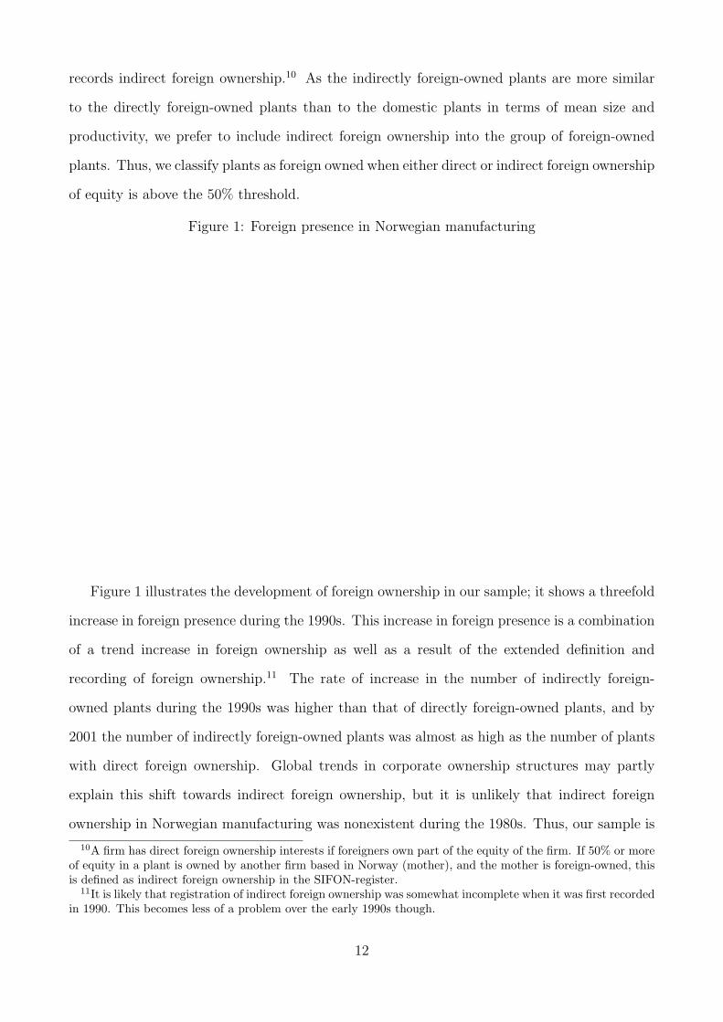
Figure 1: Foreign presence in Norwegian manufacturing
Figure 1 illustrates the development of foreign ownership in our sample; it shows a threefold
increase in foreign presence during the 1990s. This increase in foreign presence is a combination
of a trend increase in foreign ownership as well as a result of the extended definition and
recording of foreign ownership.11 The rate of increase in the number of indirectly foreign-
owned plants during the 1990s was higher than that of directly foreign-owned plants, and by
2001 the number of indirectly foreign-owned plants was almost as high as the number of plants
with direct foreign ownership. Global trends in corporate ownership structures may partly
explain this shift towards indirect foreign ownership, but it is unlikely that indirect foreign
ownership in Norwegian manufacturing was nonexistent during the 1980s. Thus, our sample is
10A firm has direct foreign ownership interests if foreigners own part of the equity of the firm. If 50% or moreof equity in a plant is owned by another firm based in Norway (mother), and the mother is foreign-owned, thisis defined as indirect foreign ownership in the SIFON-register.
11It is likely that registration of indirect foreign ownership was somewhat incomplete when it was first recordedin 1990. This becomes less of a problem over the early 1990s though.
12
likely to underestimate the extent of foreign ownership before the early 1990s. We are aware
that the extended definition of foreign ownership causes a break in our definitions of foreign
entry and foreign presence, thus, in Section 5, we check that our results are not sensitive to the
inclusion of indirect foreign ownership in the 1990s.
In the Norwegian Manufacturing Statistics each plant is assigned an identification number
which it keeps throughout its life. A plant will even keep its previous identification number
when it re-enters the panel after a time of inactivity as long as production restarts in the same
geographic location. Mergers or buy-outs at the firm level do not affect the plant identification
code. Since our data are from a census, we avoid the problem of possible false entries and exits
due to plants not being sampled. We define a plant as an entrant in year t if it appears for the
first time in year t, or reappears in that year after a temporary closure.12 Similarly we define
an exit in year t if the plant is present in year t and temporarily closed in t + 1, or absent all
subsequent years.
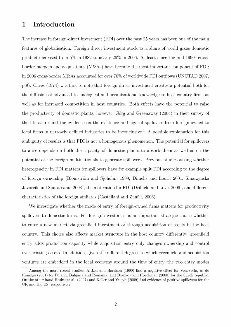
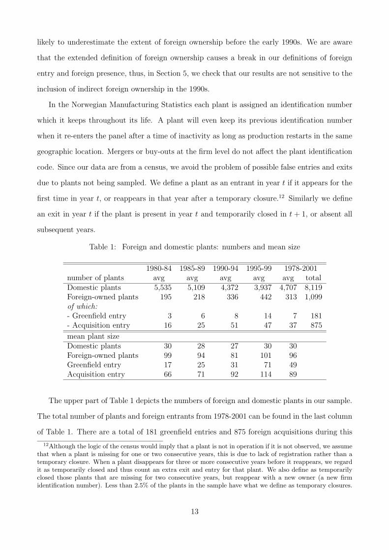
Table 1: Foreign and domestic plants: numbers and mean size
1980-84 1985-89 1990-94 1995-99 1978-2001number of plants avg avg avg avg avg totalDomestic plants 5,535 5,109 4,372 3,937 4,707 8,119Foreign-owned plants 195 218 336 442 313 1,099of which:- Greenfield entry 3 6 8 14 7 181- Acquisition entry 16 25 51 47 37 875
mean plant sizeDomestic plants 30 28 27 30 30Foreign-owned plants 99 94 81 101 96Greenfield entry 17 25 31 71 49Acquisition entry 66 71 92 114 89
The upper part of Table 1 depicts the numbers of foreign and domestic plants in our sample.
The total number of plants and foreign entrants from 1978-2001 can be found in the last column
of Table 1. There are a total of 181 greenfield entries and 875 foreign acquisitions during this
12Although the logic of the census would imply that a plant is not in operation if it is not observed, we assumethat when a plant is missing for one or two consecutive years, this is due to lack of registration rather than atemporary closure. When a plant disappears for three or more consecutive years before it reappears, we regardit as temporarily closed and thus count an extra exit and entry for that plant. We also define as temporarilyclosed those plants that are missing for two consecutive years, but reappear with a new owner (a new firmidentification number). Less than 2.5% of the plants in the sample have what we define as temporary closures.
13
period, and we observe 1,099 distinct foreign-owned plants. The remaining columns show the
annual average number of plants over the whole period and different subperiods. During the
period of analysis the number of domestic plants in our sample decreased from an average of
5,535 per year before 1985 to an average of 3,937 plants per year during the 1995-1999 period.
This reflects the overall decline in the manufacturing sector during this period. The lower part
of Table 1 shows the mean size of the different groups of plants. As expected, the foreign-owned
plants are larger than the domestic plants. Even the foreign greenfield entrants are on average
larger than domestic plants.13
For the econometric analysis we clean the data with respect to missing observations and
outliers. We drop plants with missing information on inputs or output for 80% or more of their
life. We also drop all observations of plants with one or more observations on profit margins
in the top or bottom half percentile. This cleaning procedure drops 10% of the observations
in the initial sample. In our regressions we look at the effect of foreign presence and foreign
entry on the productivity of plants that have less than 20% foreign ownership throughout their
presence in our sample (hereafter called domestic plants). Summary statistics of the regression
variables are presented in Table 6 in the Appendix.
5 Results
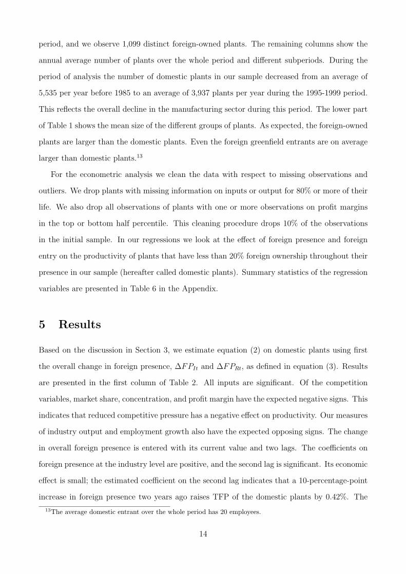
Based on the discussion in Section 3, we estimate equation (2) on domestic plants using first
the overall change in foreign presence, ∆FPIt and ∆FPRt, as defined in equation (3). Results
are presented in the first column of Table 2. All inputs are significant. Of the competition
variables, market share, concentration, and profit margin have the expected negative signs. This
indicates that reduced competitive pressure has a negative effect on productivity. Our measures
of industry output and employment growth also have the expected opposing signs. The change
in overall foreign presence is entered with its current value and two lags. The coefficients on
foreign presence at the industry level are positive, and the second lag is significant. Its economic
effect is small; the estimated coefficient on the second lag indicates that a 10-percentage-point
increase in foreign presence two years ago raises TFP of the domestic plants by 0.42%. The
13The average domestic entrant over the whole period has 20 employees.
14

coefficients on foreign presence at the region level have different signs, the contemporaneous
coefficient reaches significance at the 10% level. This implies that a 10 percentage point increase
in foreign presence in the current year reduces the productivity of domestic firms in the same
region by 0.39%. In the row with∑
∆FP we sum the three coefficients on the change in foreign
presence: the cumulative effect at the industry level is positive and significant. The cumulative
effect at region level is negative but not significant. Note that the economic effect of foreign
presence at the industry level is similar to that estimated by Haskel et al. (2007); they find
that a 10 percentage point increase in foreign presence in a U.K. industry raises the TFP of
that industry’s domestic plants by about 0.5%. They do not find an effect at the region level.
As argued earlier, this measure of overall foreign presence combines the effects from recent
foreign entrants and from foreign firms that have been present for more than one year. In
addition, the overall foreign presence term cannot distinguish between different modes of foreign
entry. The small effects of overall foreign presence could be the results of opposing effects of
different sources of changes in foreign presence. To examine this, we split the overall change
in foreign presence according to equation (4). The results are presented in columns 2-4 of
Table 2. In order to demonstrate that the coefficients on foreign entry at the industry level
are independent of the coefficients on foreign entry at the region level, column 2 contains only
industry-level entry rates and column 3 contains only region-level industry rates. In column
4 both types of entry rates are included jointly. In all three columns with foreign entry the
coefficients on inputs and controls are almost identical to those in the equations with overall
foreign presence.14 The coefficients on greenfield entry at industry level are negative, with
contemporaneous greenfield entry and its first lag being significant at the 10 and 1% level,
respectively. Their cumulative effect is also negative and significant. For greenfield entry we
also find the first lag at the labour market region level to be negative and significant; the joint
effect at the region level is also negative and significant. Regarding acquisitions, at the industry
level all three coefficients are positive, but only the first lag is significant; their cumulative effect
14As is common in this type of regression most of the variation is explained by the inputs. The year andindustry dummies add about 2 percentage points, the competition variables and the terms for foreign pres-ence/foreign entry each add less than 1 percentage point of explanatory power. If the competition variables orindustry growth rates are excluded from any of these regressions, the results do not change beyond minor upsor downs past the first digit.
15
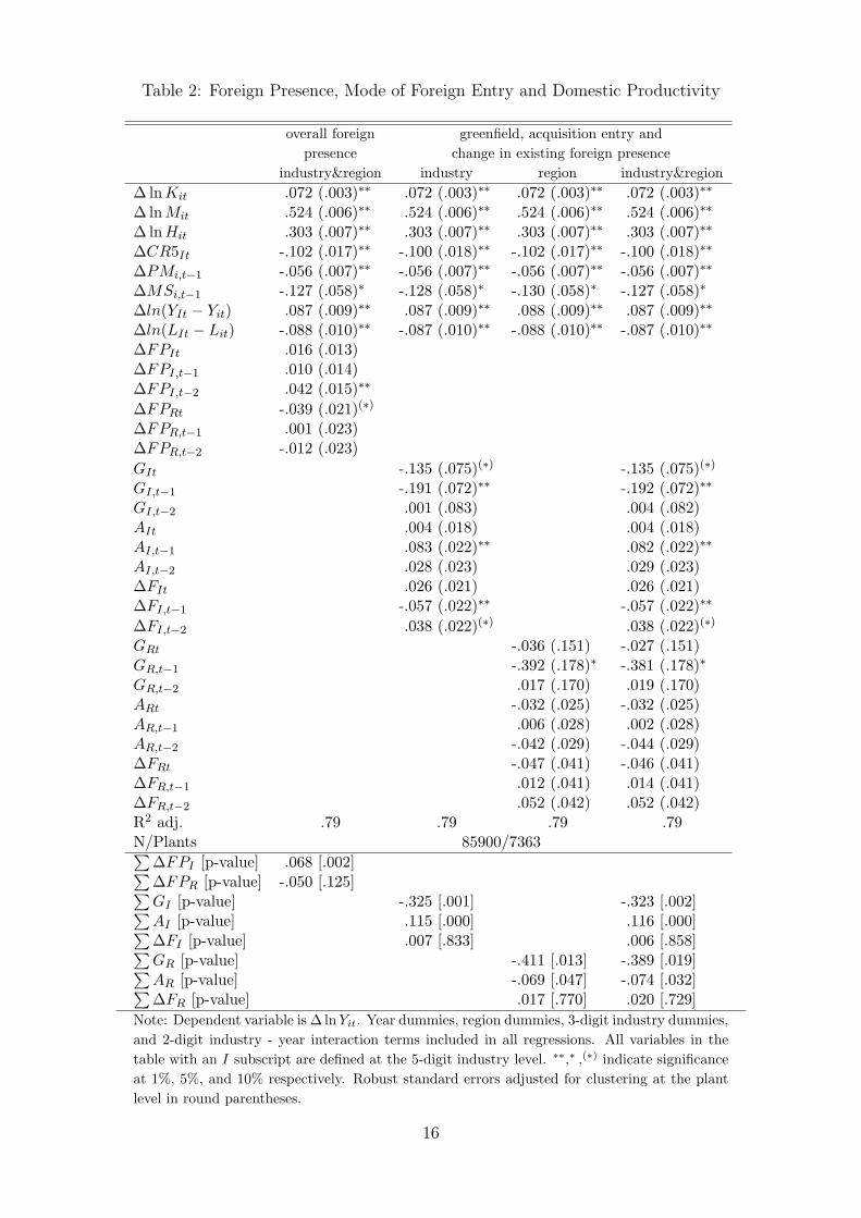
Table 2: Foreign Presence, Mode of Foreign Entry and Domestic Productivity
overall foreign greenfield, acquisition entry andpresence change in existing foreign presence
industry®ion industry region industry®ion∆lnKit .072 (.003)∗∗ .072 (.003)∗∗ .072 (.003)∗∗ .072 (.003)∗∗
∆lnMit .524 (.006)∗∗ .524 (.006)∗∗ .524 (.006)∗∗ .524 (.006)∗∗
∆lnHit .303 (.007)∗∗ .303 (.007)∗∗ .303 (.007)∗∗ .303 (.007)∗∗
∆CR5It -.102 (.017)∗∗ -.100 (.018)∗∗ -.102 (.017)∗∗ -.100 (.018)∗∗
∆PMi,t−1 -.056 (.007)∗∗ -.056 (.007)∗∗ -.056 (.007)∗∗ -.056 (.007)∗∗
∆MSi,t−1 -.127 (.058)∗ -.128 (.058)∗ -.130 (.058)∗ -.127 (.058)∗
∆ln(YIt − Yit) .087 (.009)∗∗ .087 (.009)∗∗ .088 (.009)∗∗ .087 (.009)∗∗
∆ln(LIt − Lit) -.088 (.010)∗∗ -.087 (.010)∗∗ -.088 (.010)∗∗ -.087 (.010)∗∗
∆FPIt .016 (.013)∆FPI,t−1 .010 (.014)∆FPI,t−2 .042 (.015)∗∗
∆FPRt -.039 (.021)(∗)
∆FPR,t−1 .001 (.023)∆FPR,t−2 -.012 (.023)GIt -.135 (.075)(∗) -.135 (.075)(∗)
GI,t−1 -.191 (.072)∗∗ -.192 (.072)∗∗
GI,t−2 .001 (.083) .004 (.082)AIt .004 (.018) .004 (.018)AI,t−1 .083 (.022)∗∗ .082 (.022)∗∗
AI,t−2 .028 (.023) .029 (.023)∆FIt .026 (.021) .026 (.021)∆FI,t−1 -.057 (.022)∗∗ -.057 (.022)∗∗
∆FI,t−2 .038 (.022)(∗) .038 (.022)(∗)
GRt -.036 (.151) -.027 (.151)GR,t−1 -.392 (.178)∗ -.381 (.178)∗
GR,t−2 .017 (.170) .019 (.170)ARt -.032 (.025) -.032 (.025)AR,t−1 .006 (.028) .002 (.028)AR,t−2 -.042 (.029) -.044 (.029)∆FRt -.047 (.041) -.046 (.041)∆FR,t−1 .012 (.041) .014 (.041)∆FR,t−2 .052 (.042) .052 (.042)R2 adj. .79 .79 .79 .79N/Plants 85900/7363∑
∆FPI [p-value] .068 [.002]∑∆FPR [p-value] -.050 [.125]∑GI [p-value] -.325 [.001] -.323 [.002]∑AI [p-value] .115 [.000] .116 [.000]∑∆FI [p-value] .007 [.833] .006 [.858]∑GR [p-value] -.411 [.013] -.389 [.019]∑AR [p-value] -.069 [.047] -.074 [.032]∑∆FR [p-value] .017 [.770] .020 [.729]
Note: Dependent variable is ∆ ln Yit. Year dummies, region dummies, 3-digit industry dummies,and 2-digit industry - year interaction terms included in all regressions. All variables in thetable with an I subscript are defined at the 5-digit industry level. ∗∗,∗ ,(∗) indicate significanceat 1%, 5%, and 10% respectively. Robust standard errors adjusted for clustering at the plantlevel in round parentheses.
16

is positive and significant. At the region level none of the individual coefficients are significant,
but their joint effect is negative and significant. Our estimates imply that a ten percentage point
increase in the greenfield entry rate in a particular industry one year ago is associated with a
decrease in the productivity of the domestic plants in that industry of 1.9%. A similar increase
in last year’s acquisition rate is associated with an increase in productivity of 0.8% for the
domestic plants in that industry.15 In addition, a 10 percentage point increase in the greenfield
entry rate in a particular region last year is associated with a reduction in the productivity of
domestic plants in that labour market region by 3.8%.
The effect of the change in preexisting foreign presence, ∆FI , is somewhat ambiguous.
The first lag is negative and significant at the 1% level, whereas the two other coefficients are
positive, the second lag reaching significance at the 10% level. The cumulative effect of the
∆FI-terms is close to zero and not significant. At the region level none of the coefficients on
the change in preexisting foreign presence are significant. The fact that it is always the first
lag that has a significant sign for each component of foreign presence might suggest a degree
of multicollinearity. However, when we enter each of the 18 foreign entry terms individually,
when we enter only contemporaneous, only first or only second lags together or when we enter
only the terms for one type of foreign investment at a time, the results are very similar. These
results are displayed in Tables 7 and 8 in the Appendix.
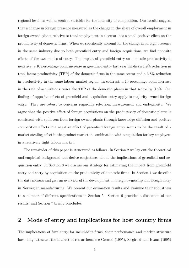
There are a number of estimation issues that we need to address in order to assess the ro-
bustness of our main finding that greenfield foreign entry and foreign entry through acquisitions
give rise to opposite effects on the productivity of domestic firms in the same sector. In what
follows we present results where we change the definition of foreign ownership and the measures
of productivity. We also address the possibility of selection bias and endogeneity.
Definition of foreign ownership
As noted in Section 4, from 1990 onwards our definition of foreign ownership includes both
directly and indirectly foreign-owned plants. This might suggest that some of the foreign entry
in our estimations is due to reclassifications rather than actual foreign entry. To address this,
15The difference between these two effects is statistically significant at the 1% level.
17

we estimate equation (2) with the foreign entry and acquisition variables based on direct foreign
ownership which we observe throughout the period. We obtain the results shown in the first
column of Table 3. Here it is the second lag of greenfield entry at the industry level that is
negative and significant, but overall the results are similar to those in our basic regression in
column 4 of Table 2. Thus our results do not seem sensitive to the extended definition of foreign
ownership in the 1990s.
In our base results plants are considered to be foreign if 50% or more of equity is directly or
indirectly controlled by foreign owners. In column 2 of Table 3 we reduce this threshold to 20%.
With this specification we do not measure a negative effect from greenfield entry at the industry
level, while the negative effect from greenfield entry in the same region persists. The coefficients
on acquisition entry are jointly significant and positive and there is a positive effect from the
change in preexisting foreign presence at the industry level. Most foreign entrants in Norwegian
manufacturing hold a majority stake in their subsidiaries, less than one third of foreign-owned
plants have below 50% foreign ownership. This makes the results for the minority foreign-owned
entrants (20-50% ownership) much more sensitive to the exclusion of certain industries, while
the results for foreign ownership defined above 50% remain qualitatively the same irrespective
of which 2-digit industry we exclude. Previous work examining whether the extent of spillovers
from foreign presence depends on the degree of ownership is inconclusive. Blomstrom and
Sjoholm (1999) conclude that the extent of spillovers is not different from minority and majority
foreign-owned firms in Indonesia, while Dimelis and Louri (2002) find that spillovers to domestic
firms in the same sector are most prominent from minority foreign-owned firms in Greece.
From 1991 onwards we have information on the exact share of foreign ownership, for this
period we define foreign ownership at the 100% level as well. For the foreign entries after
1990, 86 and 72% of, respectively, the greenfield and acquisition entrants with majority foreign
ownership are fully foreign owned. If we increase the foreign ownership threshold to 100%
as in column 3 of Table 3, our results are similar to before. Therefore the opposite effects
on domestic productivity that we obtain are not due to a differences in the extent to which
greenfield and acquisition entrants choose to take a 100% share of foreign ownership. The
differences in the results for greenfield entry at the industry level depending on whether we
18
Tab
le3:
Defi
nit
ion
offo
reig
now
ner
ship
,se
lect
ion,en
dog
enei
ty
dire
ct20
%fo
reig
n10
0%fo
reig
nH
eckm
aneff
ect
onex
cl.
ind.
-yea
rex
cl.
reg.
-yea
rfo
reig
now
ners
hip
owne
rshi
pse
lect
ion
surv
ivin
gce
llsw
ith
only
gree
nfiel
dor
owne
rshi
pth
resh
old
from
1991
mod
elpl
ants
only
acqu
isit
ion
entr
yG
It
-.09
3(.
178)
-.04
3(.
057)
-.21
8(.
082)∗∗
-.08
2(.
080)
-.12
0(.
083)
-.52
8(.
220)∗
-.03
5(.
088)
GI,t−1
-.21
4(.
180)
.002
(.04
5)-.21
1(.
075)∗∗
-.21
0(.
072)∗∗
-.18
8(.
074)∗
-.18
7(.
080)∗
-.23
0(.
081)∗∗
GI,t−2
-.38
0(.
166)∗
.106
(.06
7).0
50(.
085)
.036
(.08
8).0
64(.
088)
.109
(.09
0).0
50(.
100)
AIt
.017
(.02
3)-.00
3(.
015)
.054
(.02
7)∗
.001
(.01
8).0
04(.
022)
.082
(.05
8).0
26(.
022)
AI,t−1
.045
(.02
5)(∗
).0
21(.
016)
.092
(.03
4)∗∗
.077
(.02
3)∗∗
.035
(.02
5).0
42(.
027)
.068
(.02
6)∗∗
AI,t−2
.006
(.02
8).0
23(.
018)
.025
(.03
0).0
09(.
025)
.026
(.02
2)-.00
5(.
027)
.043
(.03
2)∆
FIt
.027
(.02
1).0
26(.
017)
.032
(.03
1).0
04(.
021)
-.03
0(.
026)
.013
(.02
7).0
17(.
027)
∆F
I,t−1
-.07
7(.
024)∗∗
-.01
4(.
015)
-.11
6(.
034)∗∗
-.04
6(.
023)∗
-.00
5(.
025)
-.07
3(.
028)∗∗
-.06
4(.
027)∗
∆F
I,t−2
.043
(.02
6)(∗
).0
32(.
016)∗
.053
(.03
6).0
30(.
022)
-.01
9(.
028)
.034
(.02
6).0
29(.
028)
GR
t.0
42(.
181)
-.16
5(.
100)
(∗)
-.15
5(.
171)
-.02
6(.
162)
-.07
0(.
196)
-.04
6(.
175)
-.12
6(.
269)
GR
,t−1
-.38
4(.
214)
(∗)
-.14
0(.
083)
(∗)
-.42
1(.
193)∗
-.31
4(.
178)
(∗)
-.25
4(.
202)
-.42
7(.
199)∗
-.38
0(.
207)
(∗)
GR
,t−2
-.00
7(.
190)
.065
(.09
2)-.13
0(.
190)
-.13
7(.
188)
.168
(.18
5).1
75(.
182)
.029
(.19
1)A
Rt
-.01
7(.
048)
.002
(.01
4)-.10
8(.
045)∗
-.04
1(.
027)
-.02
3(.
031)
-.04
7(.
029)
-.10
3(.
054)
(∗)
AR
,t−1
-.05
4(.
045)
.013
(.01
6)-.01
4(.
054)
.013
(.02
9).0
26(.
034)
.009
(.03
2).0
03(.
033)
AR
,t−2
-.02
6(.
050)
-.01
8(.
016)
-.07
7(.
041)
(∗)
-.04
0(.
031)
-.08
4(.
038)∗
-.06
7(.
034)
(∗)
-.02
5(.
032)
∆F
Rt
.070
(.04
9).0
22(.
018)
-.04
6(.
034)
-.03
9(.
044)
-.01
9(.
049)
-.02
3(.
053)
-.05
5(.
052)
∆F
R,t−1
-.02
9(.
048)
-.01
5(.
018)
-.03
3(.
035)
-.00
1(.
042)
.000
(.05
3).0
13(.
050)
.046
(.05
1)∆
FR
,t−2
.034
(.04
4).0
11(.
017)
-.00
9(.
039)
.021
(.04
2).0
01(.
056)
.049
(.04
7).0
58(.
049)
adjR
2/χ
2.7
9.7
9.7
715
.91
.74
.79
.78
ρ-.06
4(.
016)
N85
900
8590
031
330
8590
038
892
6353
357
623
Pla
nts
7363
7363
4572
7363
1852
7165
7013
∑G
I[p
-val
ue]
-.68
7[.0
06]
.066
[.439
]-.37
8[.0
00]
-.25
6[.0
13]
-.24
4[.0
15]
-.60
6[.0
13]
-.21
5[.1
06]
∑A
I[p
-val
ue]
.068
[.038
].0
40[.0
62]
.171
[.000
].0
87[.0
01]
.065
[.027
].1
18[.0
75]
.137
[.000
]∑
∆F
I[p
-val
ue]
-.00
7[.8
34]
.043
[.096
]-.03
1[.5
13]
-.01
2[.7
03]
-.05
4[.1
62]
-.02
6[.5
27]
-.01
9[.6
63]
∑G
R[p
-val
ue]
-.35
0[.1
03]
-.23
9[.0
44]
-.70
6[.0
00]
-.47
7[.0
06]
-.15
6[.4
46]
-.29
7[.1
79]
-.47
8[.0
58]
∑A
R[p
-val
ue]
-.09
7[.1
34]
-.00
3[.8
74]
-.19
9[.0
04]
-.06
8[.0
57]
-.08
1[.0
61]
-.10
5[.0
24]
-.12
5[.0
42]
∑∆
FR
[p-v
alue
].0
74[.2
16]
.017
[.515
]-.08
7[.1
13]
-.01
9[.7
43]
-.01
8[.8
02]
.039
[.595
].0
49[.5
15]
Note
:D
ependent
vari
able
is∆
lnY
it.
Regre
ssors
∆ln
Kit,
∆ln
Mit,
∆ln
Hit,
∆M
Si,t−
2,
∆P
Mi,t−
2,
∆C
R5
I,t
,∆
ln(Y
It−
Yit),
∆ln
(LI
t−
Lit)
as
well
as
year
dum
mie
s,re
gio
ndum
mie
s,
3-d
igit
indust
rydum
mie
s,and
2-d
igit
-year
inte
racti
on
term
sare
inclu
ded
but
not
dis
pla
yed
for
bre
vity.∗∗
,∗,(∗)
indic
ate
signifi
cance
at
1%
,5%
,and
10%
resp
ecti
vely
.R
obust
standard
err
ors
adju
sted
for
clu
steri
ng
at
the
pla
nt
levelin
round
pare
nth
ese
s.Sele
cti
on
inth
efirs
tst
age
ofth
ere
gre
ssio
nin
colu
mn
3is
dete
rmin
ed
by
capit
aland
invest
ment
(levels
to4th
pow
ers
).χ2
isth
e
test
stati
stic
for
the
join
tsi
gnifi
cance
ofth
evari
able
sin
the
sele
cti
on
equati
on.
ρis
the
sele
cti
on
term
.χ2
isth
ete
stst
ati
stic
for
the
join
tsi
gnifi
cance
ofth
evari
able
sin
the
sele
cti
on
equati
on.
ρis
the
sele
cti
on
term
.
19
define foreign ownership at the 20%, 50% or 100% threshold point in the same direction as the
results of Smarzynska Javorcik and Spatareanu (2008) for Romania. They conclude that the
negative competition effect is smaller from jointly owned enterprises than from fully foreign-
owned enterprises, they do not distinguish between greenfield and acquisition entry, however.
Selection
As the variables of main interest are foreign entry, we should take into account that the esti-
mated relationship between these variables and productivity could be biased by selection on
survival. Suppose for example, that both modes of foreign entry truly have a positive effect on
the productivity of domestic firms, or that foreign entry occurs primarily in sectors with good
market growth prospects. In such sectors, even low productivity firms may survive, creating a
negative correlation between foreign entry and productivity among surviving firms. If this is the
case we would be underestimating the positive effects of foreign acquisitions, and overstating
the negative effect of greenfield entry. Conversely, if foreign entry increases competitive pres-
sure such that the least productive domestic firms in the sector exit as a result of foreign entry,
there will be a positive correlation between foreign entry and productivity among surviving
firms. Thus, selection could work in both directions and the overall bias is unknown.
To address this potential problem we re-estimate the model from the second column using
the Heckman selection procedure where survival is conditioned on a probit of so-called haz-
ard variables that determine exit. Olley and Pakes (1996) suggest a structural model where
survival is conditioned on investment and capital. This is to capture the idea that investment
which is observable but not correlated with current output can pick up unobservable shocks to
productivity. The result from using investment and capital from levels to their fourth powers
as selection variables in a Heckman selection model to capture the Olley and Pakes idea is pre-
sented in column 4 of Table 3. The results are very similar to those in our original specification
in column 4 of Table 2 without the selection correction. The variables in the selection probit
are jointly significant, as indicated by the χ2-value. The selection term ρ is also significant.
Another way to gauge whether our results are biased by selection is to note that if most of
the adjustment to foreign entry is at the exit margin, we should expect a much smaller effect
20

of foreign entry on the surviving firms. When we restrict the sample to only those domestic
firms that are present for the entire period from 1978 to 2001 we obtain the results presented
in column 5 Table 3. The number of plants reduces to one quarter of the original sample and
the sample size to less than half. The results for greenfield entry at the industry level are
remarkably similar to the original specification in Table 2, indicating that the surviving plants
carry the largest share of the adjustment to greenfield entry. In contrast, none of the coefficients
on foreign entry by acquisition in the same sector is significant and their joint effect is smaller
in this sample of survivors than in the main sample. This suggests that some of the benefit
from foreign acquisitions goes to new domestic entrants.
Endogeneity of the mode of entry
The mode of entry into a new market is a strategic variable for multinationals, thus it could be
the case that the foreign entrants’ choice of which industry or region to enter or which firm to
acquire depends on the current or future expected performance of plants in that industry. Any
systematic correlation between mode of entry and the level of industry or region productivity
is removed by taking first differences, moreover we control fore changes in industry output and
employment growth. Thus our results cannot be explained by greenfield entrants systematically
entering in low-productivity industries or regions and acquisitions predominantly taking place in
high-productivity industries or regions. The use of year dummies and industry-year interaction
terms will take out any systematic correlation between the mode of entry and both aggregate
and industry-specific business cycles, while the industry and region dummies should pick up
systematic correlations between the mode of entry and industry-specific and region-specific
trends in productivity. Since our industry dummies are at a more aggregate level than our
measures of foreign entry rates and our controls for industry growth may not fully capture
changes in total factor productivity, there could still be scope for endogeneity of the mode of
entry at the 5-digit industry level. The same is true for endogeneity at the regional level.
Ideally, we would want an instrument correlated with greenfield entry but not correlated
with acquisition entry and productivity. As it is difficult to think of such an instrument, we
follow a different route to investigate whether endogeneity in the mode of entry decision could
21
explain the opposite effects of greenfield and acquisition entry. If our results are driven by
endogeneity in the mode of entry, the results would be generated by greenfield and acquisition
entry occurring in different industry-year/region-year cells. To check this possibility at the
industry level, we drop observations in 5-digit industry-year cells where we observe only one
mode of entry. At the region level we drop labour market region-year cells where we observe only
one mode of foreign entry. The results of these two checks are displayed in the last two columns
of Table 3. We are still able to identify a negative effect on the productivity of domestic plants
following foreign greenfield entry both at the industry and at the region level, and a positive
effect following acquisition entry at industry level. As in some previous regressions we also
identify a negative effect of foreign acquisitions on domestic firms in the same region. This
indicates that our results cannot be explained by endogeneity between the mode of foreign
entry and industry or regional performance.
Measurement of productivity and the mode of foreign entry
Table 4 presents the results for a number of further robustness checks where we vary the
measurement of productivity and the estimation method. The regressions are all variations
of equation (2) as reported in the last column of Table 2. In the first column, we report the
results of a more general specification of equation (2) in which we allow the coefficients on
inputs to vary across 3-digit industries by interacting the inputs with industry dummies. Our
specification in Table 2 constrains the input elasticities to be the same for all manufacturing
industries, but technological differences between industries may bias our estimates of the effects
of foreign entry. The results in column 1 of Table 4 do not suggest that this is the case, as the
effects of foreign entry and acquisitions, and the remaining change in foreign presence are very
similar to our original results both at the industry and at the region level.
Production function estimation has been shown to yield poor results when important unob-
servables that vary both across plants and over time, such as productivity shocks, are omitted.
This suggests that differencing and controlling for plant fixed effects may yield poor estimates
of input use and, moreover, it may not be sufficient to render the error term εit in equation (1)
white noise. Olley and Pakes (1996) show that such unobservable shocks can be proxied for by
22
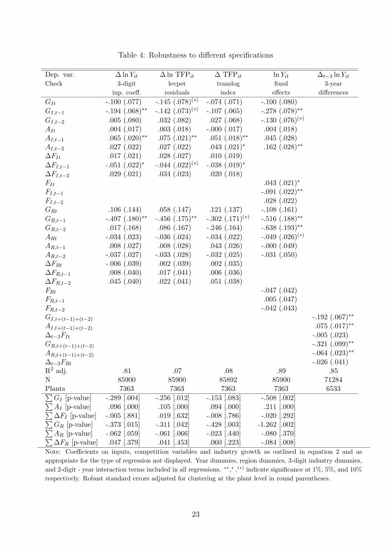
Table 4: Robustness to different specifications
Dep. var. ∆ lnYit ∆ln TFPit ∆ TFPit lnYit ∆t−3 lnYit
Check 3-digit levpet translog fixed 3-yearinp. coeff. residuals index effects differences
GIt -.100 (.077) -.145 (.078)(∗) -.074 (.071) -.100 (.080)GI,t−1 -.194 (.068)∗∗ -.142 (.073)(∗) -.107 (.065) -.278 (.078)∗∗
GI,t−2 .005 (.080) .032 (.082) .027 (.068) -.130 (.076)(∗)
AIt .004 (.017) .003 (.018) -.000 (.017) .004 (.018)AI,t−1 .065 (.020)∗∗ .075 (.021)∗∗ .051 (.018)∗∗ .045 (.028)AI,t−2 .027 (.022) .027 (.022) .043 (.021)∗ .162 (.028)∗∗
∆FIt .017 (.021) .028 (.027) .010 (.019)∆FI,t−1 -.051 (.022)∗ -.044 (.022)(∗) -.038 (.019)∗
∆FI,t−2 .029 (.021) .034 (.023) .020 (.018)FIt .043 (.021)∗
FI,t−1 -.091 (.022)∗∗
FI,t−2 .028 (.022)GRt .106 (.144) .058 (.147) .121 (.137) -.108 (.161)GR,t−1 -.497 (.180)∗∗ -.456 (.175)∗∗ -.302 (.171)(∗) -.516 (.188)∗∗
GR,t−2 .017 (.168) .086 (.167) -.246 (.164) -.638 (.193)∗∗
ARt -.034 (.023) -.036 (.024) -.034 (.022) -.049 (.026)(∗)
AR,t−1 .008 (.027) .008 (.028) .043 (.026) -.000 (.049)AR,t−2 -.037 (.027) -.033 (.028) -.032 (.025) -.031 (.050)∆FRt -.006 (.039) .002 (.039) .002 (.035)∆FR,t−1 .008 (.040) .017 (.041) .006 (.036)∆FR,t−2 .045 (.040) .022 (.041) .051 (.038)FRt -.047 (.042)FR,t−1 .005 (.047)FR,t−2 -.042 (.043)GI,t+(t−1)+(t−2) -.192 (.067)∗∗
AI,t+(t−1)+(t−2) .075 (.017)∗∗
∆t−3FIt -.005 (.023)GR,t+(t−1)+(t−2) -.321 (.099)∗∗
AR,t+(t−1)+(t−2) -.064 (.023)∗∗
∆t−3FRt -.026 (.041)R2 adj. .81 .07 .08 .89 .85N 85900 85900 85892 85900 71284Plants 7363 7363 7363 7363 6533∑
GI [p-value] -.289 [.004] -.256 [.012] -.153 [.083] -.508 [.002]∑AI [p-value] .096 [.000] .105 [.000] .094 [.000] .211 [.000]∑∆FI [p-value] -.005 [.881] .019 [.632] -.008 [.786] -.020 [.292]∑GR [p-value] -.373 [.015] -.311 [.042] -.428 [.003] -1.262 [.002]∑AR [p-value] -.062 [.059] -.061 [.066] -.023 [.440] -.080 [.370]∑∆FR [p-value] .047 [.379] .041 [.453] .060 [.223] -.084 [.008]
Note: Coefficients on inputs, competition variables and industry growth as outlined in equation 2 and asappropriate for the type of regression not displayed. Year dummies, region dummies, 3-digit industry dummies,and 2-digit - year interaction terms included in all regressions. ∗∗,∗ ,(∗) indicate significance at 1%, 5%, and 10%respectively. Robust standard errors adjusted for clustering at the plant level in round parentheses.
23
investment behavior, on the assumption that these shocks influence current investment, but -
since investment takes time - not current output. Their approach requires that plants under-
take a positive amount of investment, which is not the case for about 25% of the observations
in our sample. Instead, Levinsohn and Petrin (2003) propose using intermediate inputs rather
than investment to address the underlying simultaneity problem. We use the Levinsohn-Petrin
method to estimate total factor productivity (TFP) as the residuals of a Cobb-Douglas pro-
duction function at the 2-digit level.16 In the second column we use the first difference of this
TFP measure as our dependent variable when estimating equation (2), omitting the inputs on
the right hand side. In the third column, our measure of productivity is a superlative index of
TFP derived from a flexible translog specification of the production technology, see Caves et al.
(1982a, 1982b).17 Both the results in columns 2 and 3 are similar to our original specification.
Note, however, that in contrast to our analysis so far the TFP measures in columns 2 and 3
impose constant returns to scale.
In our main specification we eliminate unobserved time invariant effects by taking first
differences. An alternative method is to use fixed effects estimation (within-transformation)
as displayed in the fourth column of Table 4. The effect from greenfield entry is also negative
both at industry and region level. At the industry level the effect of acquisitions is positive,
while the effect of preexisting foreign presence remains ambiguous.
First differencing is known to introduce biases by exacerbating measurement error in the
regressors. Longer time differences tend to reduce this problem (Griliches and Hausman, 1986),
therefore we report the results from three-year differences in the last column of Table 4. To
make our entry measures consistent with the longer differences, we include in the GI,t+(t−1)+(t−2)-
measure all foreign greenfield entrants that entered either in the current year or in the previous
two years. The acquisition measure is defined in a similar way for plants that were acquired
by foreign owners in year t, t − 1, or t − 2. The change in remaining foreign presence is then
the 3-year difference in foreign presence minus the 3-year entry rates. The results from this
specification confirm our earlier results, greenfield entry has a negative effect on the productivity
16In the absence of an appropriate deflator we use the share of energy in material use to proxy for unobservedproductivity shocks.
17This index is used by Aghion et al. (2009). Details on the construction of this index can be found in theAppendix.
24
of domestic plants both in the same industry and in the same region. Acquisition entry has a
positive effect on the productivity of domestic plants in the same industry and here we also get
a negative effect from acquisition entry on domestic plants in the same region.
6 Discussion
The main message from the results presented in Section 5 can be summarised as follows: recent
greenfield entry in the same sector has a negative impact on the productivity of domestic plants,
while recent acquisition entry has a positive effect. Recent greenfield entry in the same region
has a negative effect, and this is also the case, but to a smaller extent, for acquisition entry in
the same region in some of our specifications. The cumulative effect of remaining changes in
preexisting foreign presence is never significant in our specifications.
Turning to the regional entry rates first, our results indicate that any positive effects of
knowledge diffusion from foreign entrants in the same region must be dominated by another
negative effect. Clearly, these entry rates do not capture product market competition since the
industry entry rates are included in the same regression. As capital goods and intermediate
inputs are more easily sourced from abroad, the most likely candidate for the negative effect
is competition in the labour market. The literature on labour mobility suggests that domestic
plants benefit from hiring employees that have experience in multinational firms (Gorg and
Strobl, 2005; Poole, 2009; Balsvik, forthc.18). When key employees move in the other direction
this may well work to the detriment of the domestic firms. Aitken et al. (1996) argue that the
productivity of the domestic firms may decrease if foreign firms poach the best workers from
domestic firms this may reduce the productivity of the domestic firms. In addition, an increased
demand for skilled labour following foreign entry may increase labour costs, and hence reduce
productivity (Barry et al., 2005).
Information on the skill composition of employees would help to shed some light on these
issues, unfortunately our data set does not contain this information. There is, however, evidence
that workers in foreign-owned firms are positively selected relative to workers in domestically
18There is also work on spillovers associated with the mobility of scientists, see among others Song et al.(2003) and Møen (2005).
25
owned plants (Balsvik, forthc.). There is also evidence that foreign-owned firms in Norwegian
manufacturing pay higher wages (Balsvik and Haller, forthc.). Norway is also a small country
with relatively low unemployment which makes it likely that the cost of loosing key employees to
foreign multinationals reduces productivity in the domestic firms affected. Given that greenfield
entrants need to hire much more staff than acquisition entrants in the initial years after entry,
it appears reasonable that the negative effect of competition at the labour market region level
is largest from greenfield entry.
Turning next to our findings on industry entry rates: the positive effect on domestic pro-
ductivity from acquisition entry is consistent with the idea of positive knowledge spillovers.
While foreign acquisitions increase competition in the longer run, in the short run the domes-
tic plants seem to be able to turn the change in ownership structure in the industry to their
advantage. This could be because the acquired plants themselves are hampered by in-house
restructuring after a takeover. Labour turnover associated with the change in ownership in the
case of foreign acquisitions may provide a pool of employees to domestic firms who serve as a
channel for knowledge diffusion. The negative effect from greenfield entry could then be due
to either competition in the labour market as discussed above and/or a negative competition
effect in the product market. Several spillover studies have found significant negative effects of
foreign presence in the same sector on domestic productivity. The most prominent explanation
proposed so far is that of a negative competition effect through market stealing (Aitken and
Harrison, 1999), whereby domestic firms lose market shares to foreign-owned firms and thus
move up their average cost curves. While our regressions control for changes in market share
and other competition variables, competition from foreign entrants may still force domestic
firms up their average cost curves if they are unable to fully adjust their input use in the short
run. In the following illustrative regressions, we concentrate on product market competition
and therefore drop the regional entry rates.
The two modes of foreign entry have a different impact on market structure, simply because
greenfield entry adds additional production capacity while a foreign acquisition merely changes
the name of an existing market share. As a result, market stealing effects should primarily come
from foreign-owned firms that are new to the market rather than from foreign acquisitions. The
26

Table 5: Effect of domestic entry on domestic productivity and effect of foreign entryon industries split by median export intensity
Dep. var. ∆ ln Yit ∆ln Yit ∆ln Yit
Check domestic industry-level export intensityentry below median above median
DEiIt -.005 (.031)DEiI,t−1 -.030 (.028)DEiI,t−2 -.032 (.030)GIt -.165 (.092)(∗) .111 (.151)GI,t−1 -.171 (.082)∗ -.189 (.183)GI,t−2 .017 (.094) -.071 (.178)AIt .016 (.028) -.024 (.026)AI,t−1 .109 (.036)∗∗ .045 (.027)(∗)
AI,t−2 .039 (.037) .053 (.027)(∗)
∆FIt .100 (.037)∗∗ -.019 (.026)∆FI,t−1 -.055 (.038) -.058 (.027)∗
∆FI,t−2 .076 (.039)∗ .009 (.027)adj R2 .78 .79 .78N/Plants 85900/7363 58645/5127 27255/2396∑
DEiI [p-value] -.066 [.053]∑GI [p-value] -.318 [.009] -.149 [.526]∑AI [p-value] .164 [.000] .075 [.051]∑∆FI [p-value] .120 [.022] -.068 [.130]
Note: Unreported regressors are ∆ ln Kit, ∆ ln Mit, ∆ ln Hit, ∆MSi,t−2,∆PMi,t−2, ∆CR5I,t as well as year dummies, region dummies, 3-digitindustry dummies, and 2-digit - year interaction terms. Columns 2 and3 also control for ∆ln(YIt − Yit) and ∆ln(LIt − Lit). ∗∗,∗ ,(∗) indicatesignificance at 1%, 5%, and 10% respectively. Robust standard errorsadjusted for clustering at the plant level in round parentheses. DEiI incolumn 1 is the employment-weighted entry rate of domestic plants atthe 5-digit industry level.
negative productivity effect of greenfield entry on domestic plants could of course be an effect
of entry in general and need not be specific to foreign greenfield entry. We check this by
estimating equation (2) using employment-weighted entry rates of domestic plants instead of
our measures of foreign entry (see the Appendix for variable definitions). As can be seen from
the first column of Table 5, none of the estimated coefficients on domestic entry are significant.
An explanation for the different effects of foreign and domestic entry is that domestic entry is
part of a regular turnover process in an industry, while foreign greenfield entry is the result
of large and successful firms expanding abroad. Thus, the market stealing effect from foreign
entrants is likely to be stronger than from domestic entrants.
27

If the negative effect from greenfield entry is a result of market stealing, firms in industries
producing mainly for the domestic market should be affected more than firms that sell a sub-
stantial share of their output in foreign markets. To examine this possibility we split the sample
at the median export intensity which in our sample is 22.2% (for a definition and data used
in the construction of the export intensity measure please consult the Appendix). The results
of these regressions are displayed in columns 2 and 3 of Table 5. Foreign acquisitions have a
positive effect irrespective of the export intensity. Instead the negative effect from greenfield
entry on domestic firms in the same industry affects only firms in industries that are focussed
mainly on the domestic market. Since our dataset does not contain plant-level output prices,
we are unable to determine whether this decline in productivity is primarily due to competition
lowering output prices or to reducing the volume of production.
7 Conclusions
Our aim in this paper is to bring new insights to the spillover debate by distinguishing between
new and existing foreign-owned firms, and moreover between different modes of foreign entry.
In our panel of Norwegian manufacturing plants, an overall change in foreign presence at the
industry level has a small positive impact on the productivity of domestic plants, while foreign
presence in the same region has a less precisely measured negative effect on the productivity
of domestic plants in that region. When decomposing the measure of industry foreign presence
into new and existing foreign firms, we find opposite effects from greenfield entrants and foreign
acquisitions. The impact of greenfield entry on the productivity of domestic plants in the same
industry is negative, while we find a positive effect from foreign acquisitions. Foreign entry
at the regional level has a negative effect on the productivity of domestic plants in the same
labour market region, strongest for greenfield entrants.
Foreign entry through greenfield investment and acquisition of domestic firms are likely
to differ both in their effect on market structure and in their effect on labour demand. The
estimated effect of foreign acquisitions on the productivity of domestic plants is consistent
with spillovers from foreign-owned plants through knowledge diffusion and positive competition
effects. Greenfield entrants add additional production capacity and are therefore more likely
28
to steal market shares from domestic plants than multinational firms that enter the domestic
market by acquisition of domestic firms. In addition, greenfield entrants must find employees
for their new production facilities, and may thus ‘poach’ key employees from domestic plants.
Competition in the labour market is likely to occur also at the regional level, as foreign-owned
plants may not only hire workers from existing plants in the same industry but also in the
same labour market region. Also plants that are acquired by foreign owners may restructure
or expand their employment, and hence may also contribute to labour stealing from domestic
plants, but at a smaller scale than greenfield entrants. Both of these effects contribute towards
explaining our results of an opposite effect of foreign acquisitions and greenfield entry on the
productivity of domestic firms. An interesting avenue for future research could, therefore, be
to examine these effects in more detail using linked employer-employee data.
References
[1] Aghion, P.; Blundell, R.; Griffith, R.; Howitt, P.; Prantl, S. (2004), ‘Entry and Produc-
tivity Growth: Evidence from Microlevel Panel Data’, Journal of the European Economic
Association 2(2-3): 265-276.
[2] Aghion, P.; Blundell, R.; Griffith, R.; Howitt, P.; Prantl, S. (2009), ‘The Effects of Entry
on Incumbent Innovation and Productivity’, Review of Economics and Statistics 91(1):
20-32.
[3] Aitken, B.J.; Harrison, A.E. (1999), ‘Do Domestic Firms Benefit from Foreign Direct
Investment? Evidence from Venezuela’, American Economic Review, 89(3): 605-618.
[4] Aitken, B.J.; Harrison, A.E.; Lipsey, R.E. (1996), ‘Wages and Foreign Ownership: A
Comparative Study of Mexico, Venezuela and the United States’, Journal of International
Economics 40(3-4): 345-371.
[5] Balsvik, R. (fortc.), ‘Is Mobility of Labour a Channel for Spillovers from Multinationals
to Local Domestic Firms?’, Review of Economics and Statistics.
29

[6] Balsvik, R.; Haller, S.A. (forthc.), ‘Picking ’lemons’ or ’cherries’? Domestic and foreign
acquisitions in Norwegian manufacturing’, Scandinavian Journal of Economics.
[7] Barba Navaretti, G.; Venables, A.J. (2004) with F. Barry, K. Ekholm, A. Falzoni, J.
Haaland, K-H. Midelfart and A. Turrini, Multinational Firms in the World Economy,
Princeton University Press: Princeton.
[8] Barry, F.; Gorg, H.; Strobl, E. (2005), ‘Foreign Direct Investment and Wages in Domestic
Firms in Ireland: Productivity Spillovers versus Labour Market Crowding Out’, Interna-
tional Journal of the Economics of Business 12(1): 67-84.
[9] Bhuller, M.S. (2009), ‘Inndeling av Norge i arbeidsmarkedsregioner’, in Norwegian, Notater
2009/24, Statistics Norway.
[10] Blomstrom, M.; Sjoholm, F. (1999), ‘Technology Transfer and Spillovers: Does Local
Participation with Multinationals Matter?’ European Economic Review 43(4-6): 915-923.
[11] Castellani, D.; Zanfei, A. (2006), Multinational Firms, Innovation and Productivity, Ed-
ward Elgar: Chelthenam.
[12] Caves, D.W.; Christensen, L.R.; Diewert, W. E. (1982a), ‘The Economic Theory of Index
Numbers and the Measurement of Input, Output and Productivity’, Econometrica 50(6):
1393-1414.
[13] Caves, D.W.; Christensen, L.R.; Diewert, W. E. (1982b), ‘Multilateral Comparisons of
Output, Input and Productivity Using Superlative Index Numbers’, Economic Journal 92:
73-86.
[14] Caves, R.E. (1974) ‘Multinational Firms, Competition, and Productivity in Host Country
Markets’, Economica 41(162): 176-193.
[15] Caves, R.E. (1998) ‘Industrial Organization and New Findings on the Turnover and Mo-
bility of Firms’, Journal of Economic Literature 36(4): 1947-1982.
[16] Criscuolo, C.; Martin, R. (2009), ‘Multinationals and US Productivity Leadership: Evi-
dence from Great Britain’, Review of Economics and Statistics 91(2): 263-281.
30

[17] Dimelis, S.; Louri, H. (2002), ‘Foreign Ownership and Production Efficiency: A Quantile
Regression Analysis’ Oxford Economic Papers 54(3): 449-469.
[18] Djankov, S.; Hoeckman, B. (2000), ‘Foreign Investment and Productivity Growth in Czech
Enterprises’, World Bank Economic Review 14(1): 49-64.
[19] Driffield, N.; Love, J.H. (2006), ‘Does the Motivation for Foreign Direct Investment Affect
Productivity Spillovers to the Domestic Sector?’ Applied Economics Quarterly 52(1): 3-27.
[20] Geroski, P.A. (1995) ‘What do we know about entry?’, International Journal of Industrial
Organization 13: 421-440.
[21] Gorg, H.; Greenaway, D. (2004), ‘Much Ado about Nothing? Do Domestic Firms Really
Benefit from Foreign Investment?’, World Bank Research Observer 19(2): 171-197.
[22] Gorg, H.; Strobl, E. (2005), ‘Spillovers from Foreign Firms through Worker Mobility: An
Empirical Investigation’, Scandinavian Journal of Economics 107: 693-709.
[23] Griliches, Z.; Hausman, J.A. (1986), ‘Errors in Variables in Panel Data’, Journal of Econo-
metrics 31: 93-118.
[24] Haller, S.A. (2009), ‘The Impact of Multinational Entry on Domestic Market Structure
and Investment’, Review of International Finance and Economics 18(1): 52-62.
[25] Harrigan, J. (1997), ‘Technology, Factor Supplies, and International Specialization: Esti-
mating the Neoclassical Model’, American Economic Review 87(4): 475-494.
[26] Harris, R.D.; Robinson. C. (2002), ‘The Effect of Foreign Acquisitions on Total Factor
Productivity: Plant-Level Evidence from U.K. Manufacturing, 1987-1992’, Review of Eco-
nomics and Statistics 84(3): 562-568.
[27] Haskel, J.E.; Pereira, S.C.; Slaughter, M.J. (2007), ‘Does Inward Foreign Direct Investment
Boost the Productivity of Domestic Firms’, Review of Economics and Statistics, 89(3):
482-496.
31
[28] Javorcik, B.; Saggi, K. (forthc.), ‘Technological Asymmetry among Foreign Investors and
Mode of Entry’, Economic Inquiry.
[29] Keller, W.; Yeaple, S. (2009), ‘Multinational Enterprises, International Trade, and Tech-
nology Diffusion: A Firm-level Analysis of the Productivity Effects of Foreign Competition
in the United States’, Review of Economics and Statistics 91(4).
[30] Konings, J. (2001), ‘The Effects of Direct Foreign Investment on Domestic Firms: Evidence
from Firm Level Panel Data in Emerging Economies’, Economics of Transition 9(3): 619-
633.
[31] Levinsohn, J.; Petrin, A. (2003), ‘Estimating Production Functions Using Inputs to Control
for Unobservables’, Review of Economic Studies 70: 317-341.
[32] Mattoo A.; Olarrega M.; Saggi, K. (2004), ‘Mode of foreign entry, technology transfers,
and FDI policy’, Journal of Development Economics 75: 95-111.
[33] McGuckin, R.H.; Nguyen, S.V. (1995), ‘On the Productivity and Plant Ownership Change:
New Evidence from the Longitudinal Research Database’, RAND Journal of Economics
26(2): 257-276.
[34] Møen, J. (2005), ‘Is Mobility of Technical Personnel a Source of R&D Spillovers?’, Journal
of Labor Economics 23: 81-114.
[35] Nickell, S. (1996), ‘Competition and Corporate Performance’, Journal of Political Economy
104(4): 724-746.
[36] Nocke, V.; Yeaple, S. (2007), ‘Cross-Border Mergers and Acquisitions versus Greenfield
Foreign Direct Investment: The Role of Firm Heterogeneity’, Journal of International
Economics 72(2): 336-365.
[37] Norback, P.-J.; Persson, L. (2008), ‘Globalization and Profitability of Cross-border Mergers
& Acquisitions’, Economic Theory 35(2): 241-266.
[38] Olley, G.S.; Pakes, A. (1996), ‘The Dynamics of Productivity in the Telecommunications
Equipment Industry’, Econometrica 64(6): 1263-1297.
32
[39] Poole, J.P. (2009), ‘Knowledge Transfers from Multinational to Domestic Firms: Evidence
from Worker Mobility’, mimeo, University of California, Santa Cruz.
[40] Raknerud, A.; Rønningen, D.; Skjerpen, T. (2007), ‘A Method for Improved Capital
Measurement by combining Accounts and Firm Investment Data’, Review of Income and
Wealth 53(3): 397-421.
[41] Sembenelli, A.; Siotis, G. (2008), ‘Foreign Direct Investment and Mark-Up Dynamics:
Evidence from Spanish Firms’, Journal of International Economics 76(1): 107-115.
[42] Siegfried, J.J.; Evans, L.B. (1995), ‘Empirical Studies of Entry and Exit: A Survey of the
Evidence’, Review of Industrial Organization 9: 121-155.
[43] Smarzynska Javorcik, B.; Spatareanu, M. (2008), ‘To Share or Not To Share: Does Local
Participation Matter for Spillovers from Foreign Direct Investment?’ Journal of Develop-
ment Economics 85(1-2): 194-217.
[44] SND, The Norwegian Industrial and Regional Development Fund, Annual reports 1993-
1999.
[45] Song, J.; Almeida, P.; Wu G. (2003), ‘Learning-by-Hiring: When Is Mobility More Likely
to Facilitate Interfirm Knowledge Transfer?’ Management Science 49(4): 351-365.
[46] Sutton, J. (1996), Sunk Costs and Market Structure, MIT Press: Cambridge and London.
[47] UNCTAD (2000), World Investment Report 2000: Cross-border Mergers and Acquisitions
and Development. United Nations: New York and Geneva.
[48] UNCTAD (2007), World Investment Report 2007: Transnational Coporations, Extractive
industries and Development. United Nations: New York and Geneva.
33

A Appendix
Table 6: Summary statistics
Variable Mean Std. Dev. Min. Max. NLevelsln Yit 9.521 1.29 2.565 15.311 85900ln Kit 7.251 1.269 1.792 12.36 85900ln Mit 8.68 1.49 1.39 14.49 85900ln Hit 3.365 1.1 -3.937 9.311 85900MSit 0.016 0.044 0 0.892 85900PMit 0.106 0.123 -0.778 0.523 85898CR5It 0.666 0.261 0.091 1 2791FPIt 0.136 0.208 0 0.962 2791FPRt 0.116 0.069 0 0.377 2791GIt 0.001 0.013 0 0.367 2791AIt 0.014 0.065 0 0.915 2791GRt 0.002 0.003 0 0.044 2791ARt 0.012 0.014 0 0.134 2791Differences∆ ln Yit -0.006 0.351 -6.203 5.308 85900∆ ln Kit 0.027 0.333 -4.395 4.527 85900∆ ln Mit 0.013 0.46 -7.014 6.791 85900∆ ln Hit -0.025 0.374 -8.066 7.293 85900∆MSit 0 0.011 -0.684 0.688 85900∆PMit -0.005 0.12 -1.119 1.004 85897∆ln(YIt − Yit) 0.009 0.189 -4.524 4.594 85900∆ln(LIt − Lit) -0.017 0.167 -4.1 4.256 85900∆FPIt 0.01 0.081 -0.554 0.942 2791∆FIt -0.006 0.049 -0.684 0.495 2791∆FPRt 0.009 0.016 -0.064 0.144 2791∆FRt -0.005 0.009 -0.064 0.053 2791
Note: Summary statistics for industry level variables are reported for5-digit industry-year cells.
34

Table 7: Individual and selected greenfield, acquisition and change in foreign presencecoefficients
individual R2 adj. contemporaneous first secondcoefficients lags only lags only lags only
GIt -.101 (.073) .79 -.091 (.074)GI,t−1 -.201 (.069)∗∗ .79 -.234 (.070)∗∗
GI,t−2 .008 (.082) .79 .015 (.083)AIt .002 (.018) .79 .003 (.018)AI,t−1 .075 (.022)∗∗ .79 .080 (.022)∗∗
AI,t−2 .031 (.022) .79 .030 (.022)∆FIt .032 (.021) .79 .030 (.022)∆FI,t−1 -.059 (.023)∗ .79 -.063 (.023)∗∗
∆FI,t−2 .052 (.022)∗ .79 .051 (.023)∗
GRt -.065 (.137) .79 -.090 (.138)GR,t−1 -.405 (.156)∗∗ .79 -.386 (.158)∗
GR,t−2 -.082 (.152) .79 -.050 (.153)ARt -.033 (.025) .79 -.034 (.025)AR,t−1 .003 (.028) .79 .000 (.028)AR,t−2 -.040 (.028) .79 -.040 (.028)∆FRt -.042 (.041) .79 -.047 (.041)∆FR,t−1 .029 (.041) .79 .019 (.041)∆FR,t−2 .053 (.041) .79 .050 (.042)R2 adj. .79 .79 .79N/Plants 85900/7363 85900/7363Note: Results in the first column are for one regression per row where only the respective foreign presencevariable is included in equation 2. Dependent variable is ∆ lnYit. Unreported regressors are ∆ lnKit,∆ ln Mit, ∆ ln Hit, ∆MSi,t−2, ∆PMi,t−2, ∆CR5I,t, ∆ln(YIt − Yit), ∆ln(LIt − Lit) as well as year dum-mies, region dummies, 3-digit industry dummies, and 2-digit - year interaction terms. ∗∗,∗ ,(∗) indicatesignificance at 1%, 5%, and 10% respectively. Robust standard errors adjusted for clustering at the plantlevel in round parentheses.
35

Tab
le8:
Gre
enfiel
d,ac
quis
itio
nan
dch
ange
info
reig
npre
sence
coeffi
cien
tsse
par
ate
for
each
type
ofen
try
GIt
-.08
6(.
073)
GI,t−1
-.19
3(.
071)∗∗
GI,t−2
.012
(.08
2)A
It
.002
(.01
8)A
I,t−1
.075
(.02
2)∗∗
AI,t−2
.031
(.02
2)∆
FIt
.025
(.02
1)∆
FI,t−1
-.04
9(.
022)∗
∆F
I,t−2
.045
(.02
2)∗
GR
t-.00
2(.
149)
GR
,t−1
-.40
2(.
175)∗
GR
,t−2
-.01
6(.
168)
AR
t-.03
2(.
025)
AR
,t−1
.002
(.02
8)A
R,t−2
-.03
9(.
028)
∆F
Rt
-.04
3(.
040)
∆F
R,t−1
.029
(.04
0)∆
FR
,t−2
.055
(.04
1)R
2ad
j..7
9.7
9.7
9.7
9.7
9.7
9N
/Pla
nts
8590
0/73
63∑
GI
[p-v
al]
-.26
8[.0
06]
∑A
I[p
-val
].1
08[.0
00]
∑∆
FI
[p-v
al]
.020
[.537
]∑
GR
[p-v
al]
-.42
0[.0
10]
∑A
R[p
-val
]-.07
0[.0
39]
∑∆
FR
[p-v
al]
.041
[.452
]N
ote:
Dep
ende
ntva
riab
leis
∆ln
Yit.
Unr
epor
ted
regr
esso
rsar
e∆
lnK
it,
∆ln
Mit,
∆ln
Hit,
∆M
Si,
t−2,
∆P
Mi,
t−2,∆
CR
5 I,t,∆
ln(Y
It−
Yit),
∆ln
(LIt−
Lit)
asw
ella
sye
ardu
mm
ies,
regi
ondu
mm
ies,
3-di
git
indu
stry
dum
mie
s,an
d2-
digi
t-
year
inte
ract
ion
term
s.∗∗
,∗,(∗)
indi
cate
sign
ifica
nce
at1%
,5%
,an
d10
%re
spec
tive
ly.
Rob
ust
stan
dard
erro
rsad
just
edfo
rcl
uste
ring
atth
epl
ant
leve
lin
roun
dpa
rent
hese
s.
36
Data and Variable Definitions
CR5It Joint market share of the 5 largest plants in a 5-digit industry in terms of output relative
to industry output.
DEiIt Domestic entry rate in 5-digit industry I. Defined as the total employment of domestic
entrants (plants with below 20% foreign ownership) in the industry divided by the total
employment of all domestic plants apart from plant i in the industry. If plant i is itself
an entrant in year t its employment is also excluded from the numerator of the domestic
entry rate.
export intensity Export intensity is defined at the 3-digit industry level as the total exports
of firms in the industry divided by the total output of firms in the industry. This is based
on firm-level export data from 1996-1998. We use the average export intensity for each
sector in these years as a proxy for the whole period of analysis.
Hit Number of person hours in the plant. Since only blue-collar hours are reported prior to 1983,
and only total hours from 1983, we estimate total hours before 1983 by using information
on the blue-collar share of the total wage bill. Rented labour hours are calculated from
the costs of rented labour using the calculated average wage for own employees.
Kit Our estimate of capital services uses the following aggregation:
Kit = Rit + (0.07 + δm)V mit + (0.07 + δb)V b
it,
where Rit is the cost of rented capital in the plant, V mit and V b
it are the estimated values
of machinery and buildings at the beginning of the year, δm = 0.06 and δb = 0.02 are
the depreciation rates that we use. We take the rate of return to capital to be 0.07. The
estimated values of buildings and machinery are obtained from information on fire insur-
ance values. To reduce noise and avoid discarding too many observations with missing
fire insurance values, we smooth these values using the perpetual inventory method. Fire
insurance values are not recorded after 1995, thus from 1996 we estimate capital values
by adding investments and taking account of depreciation. Where possible, we also use
37
estimates of firm level capital values (distributed to the plant level according to employ-
ment shares) as starting values for plants with entry after 1995. These capital values are
obtained from recent work to improve on capital estimates in Norwegian manufacturing
(see Raknerud et al. 2007). We experimented with allocating sectoral capital stock data
from the National Accounts to the plant level based on the plant’s share of energy use.
Basing the start values for capital on the plant’s shares in industry capital stock combined
with plant investment data does not alter our results qualitatively. We use separate price
deflators for investment in buildings and machinery obtained from Statistics Norway. The
aggregation level for the price deflators is according to the sector classification used in
the National Accounts, which is somewhere in between the 2- and 3-digit ISIC level.
Lit Plant employment.
Mit Total cost of materials used. We subtract the included rented labour and capital and
allocate them to the labour and capital measures respectively. We use an input price
deflator obtained from Statistics Norway. The aggregation level for the price deflator is
according to the sector classification used in the National Accounts, which is somewhere
in between the 2- and 3-digit ISIC level.
MSit Plant output as a share of 5-digit industry output.
PMit Output less material and wage costs divided by output.
∆TFPit The measure of TFP is derived from a flexible translog specification of the production
technology.
∆TFPit = ∆ ln Yit −∑
z=M,K,H
αzit∆ ln xz
it, (5)
where xzit is the quantity used of factor z in plant i at time t. The Divisia share αz
it
is defined as αzit = (αz
it + αzit−1)/2 where αz
it is the cost share of factor z relative to
total output value Y in plant i at time t. We impose constant returns to scale. Since
there could be substantial noise in the observed factor shares, αzit, we apply a smoothing
procedure proposed by Harrigan (1997). Assuming a translog production technology,
constant returns to scale (CRS), and standard market-clearing conditions, αzit can be
38
expressed as follows:
αzit = νi + ϕIt +
∑z=M,H
ωIt ln(xz
it
xKit
) (6)
where νi is a plant-specific constant, ϕIt an industry-time-specific constant and capital
use is normalised to impose CRS. If the observed factor shares deviate from the left-hand
side of this equation by an i.i.d. measurement error term, then the parameters can be
estimated by separate fixed effects panel data regressions for each industry I. We estimate
equation (6) separately for each 3-digit ISIC industry, and use the fitted values from (6)
as the factor shares in the calculation of (5).
Yit Gross production value net of sales taxes and subsidies. Deflated using an output price
deflator obtained from Statistics Norway with a level of aggregation somewhere in between
the 2- and 3-digit ISIC level.
39